lecture 2: neoclassical growth theory acemoglu …lecture 2: neoclassical growth theory (acemoglu...

Lecture 2: Neoclassical Growth Theory(Acemoglu 2009, Chapter 8)adapted from Fabrizio Zilibotti

Kjetil Storesletten

September 1, 2014

Kjetil Storesletten () Lecture 2 September 1, 2014 1 / 57

Introduction

Ramsey or Cass-Koopmans model:differs from the Solow model insofar as it explicitlymodels the consumer side and endogenizes savings

Beyond its use as a basic growth model,it is also a workhorse for many areas of macroeconomics

Example: real and monetary business cycle theory

Kjetil Storesletten (University of Oslo) Lecture 2 September 1, 2014 2 / 57

Preferences, Technology and Demographics I

Infinite-horizon, continuous time.

Representative household with instantaneous utility function

u (c (t)) ,

Assumption u (c) is strictly increasing, concave, twice continuouslydifferentiable with derivatives u′ and u′′, and satisfiesthe following Inada type assumptions:

limc→0

u′ (c) = ∞ and limc→∞

u′ (c) = 0.

Suppose representative household representsset of identical households (normalized to 1)

Each household has an instantaneous utility function u (c (t))

L (0) = 1 andL (t) = exp (nt)


Preferences, Technology and Demographics IIAll members of the household supply their labor inelasticallyObjective function of the representative household at t = 0:

U (0) ≡∫ ∞

0exp (−ρt) · L (t) · u (c (t)) dt (1)

=∫ ∞

0exp (− (ρ− n) t) · u (c (t)) dt,

whereI c (t)=consumption per capita at t,I ρ=subjective discount rate, so that effective discount rate is ρ− n.

Objective function (1) embeds:I Household is fully altruistic towards all of its future members,and makes allocations of consumption(among household members) cooperatively

I Strict concavity of U (·)

Thus each household member has an equal consumption, c (t) ≡ C (t)L(t)


Preferences, Technology and Demographics III

Assumption: ρ > n

Benchmark model without any technological progress

Factor and product markets are competitive

Production possibilities set of the economy is represented by

Y (t) = F [K (t) , L (t)] ,

F features constant returns to scale and Inada conditions, i.e.,Y = FK ·K + FL · L (Euler Theorem) andlimK→0 FK = limL→0 FL = ∞, limK→∞ FK = limL→∞ FL = 0


Preferences, Technology and Demographics IV

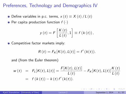
Define variables in p.c. terms, x (t) ≡ X (t) /L (t)Per capita production function f (·)

y (t) = F[K (t)L (t)

, 1]≡ f (k (t)) ,

Competitive factor markets imply:

R (t) = FK [K (t), L(t)] = f′ (k(t)).

and (from the Euler theorem)

w (t) = FL[K (t), L(t)] =F [K (t), L(t)]

L (t)− FK [K (t), L(t)]

K (t)L (t)

= f (k (t))− k (t) f ′ (k(t)).


Preferences, Technology and Demographics V

Denote asset holdings of the representative household at time t byA (t). Then,

A (t) = r (t)A (t) + w (t) L (t)− c (t) L (t)

r (t) is the market flow rate of return on assets, and w (t) L (t) is theflow of labor income earnings of the household.

Defining per capita assets as

a (t) ≡ A (t)L (t)

,

we obtain:

a (t) = (r (t)− n) a (t) + w (t)− c (t)

Household assets can consist of capital stock, K (t),which they rent to firms and bonds in zero net supply, B (t).


Preferences, Technology and Demographics VI

Given no uncertainty, arbitrage implies that the rateof return on bonds must equal the net return on capital(after depreciation at the rate δ).

Both returns must equal r (t) ⇒

r (t) = R (t)− δ

Moreover, market clearing ⇒

a (t) = k (t)


The Budget Constraint I

Let us return to the flow (or dynamic) budget constraint

a (t) = (r (t)− n) a (t) + w (t)− c (t)

Imposing that the flow constraint holds for all t ∈ [0,∞[is not suffi cient to ensure that a proper budget constrainthold unless we impose a lower bound on assets

A dynasty could increase its consumptionby running an ever growing debt


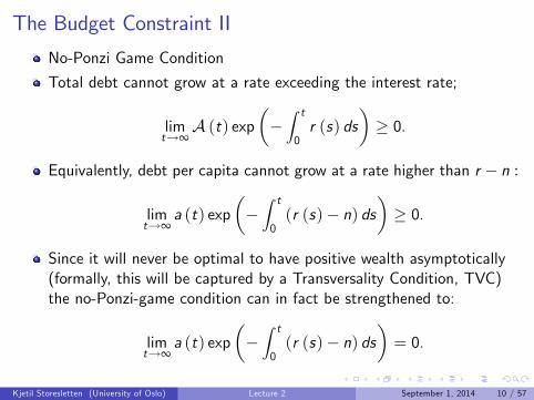
The Budget Constraint II

No-Ponzi Game Condition

Total debt cannot grow at a rate exceeding the interest rate;

limt→∞A (t) exp

(−∫ t

0r (s) ds

)≥ 0.

Equivalently, debt per capita cannot grow at a rate higher than r − n :

limt→∞

a (t) exp(−∫ t

0(r (s)− n) ds

)≥ 0.

Since it will never be optimal to have positive wealth asymptotically(formally, this will be captured by a Transversality Condition, TVC)the no-Ponzi-game condition can in fact be strengthened to:

limt→∞

a (t) exp(−∫ t

0(r (s)− n) ds

)= 0.


The Budget Constraint III

The no-Ponzi Game rules out the possibility for agentsto borrow to finance present consumption and then usefuture borrowings to roll over the debt and pay the interest

It can be shown formally (see textbook for a proof) thatthe no-Ponzi-game condition + period budget constraintensures that the individual’s lifetime budget constraint holds ininfinite horizon∫ ∞

0c (t) exp

(−∫ t

0(r (s)− n) ds

)dt

= a (0) +∫ ∞

0w (t) exp

(−∫ t

0(r (s)− n) ds

)dt


Definition of Equilibrium

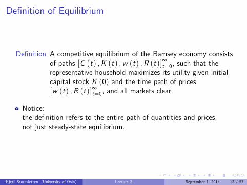
Definition A competitive equilibrium of the Ramsey economy consistsof paths [C (t) ,K (t) ,w (t) ,R (t)]∞t=0, such that therepresentative household maximizes its utility given initialcapital stock K (0) and the time path of prices[w (t) ,R (t)]∞t=0, and all markets clear.

Notice:the definition refers to the entire path of quantities and prices,not just steady-state equilibrium.


Household Maximization I

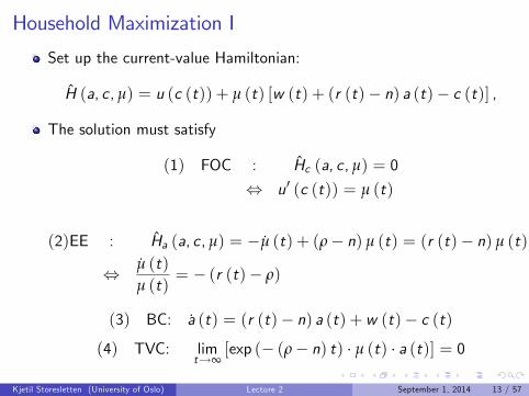
Set up the current-value Hamiltonian:

H (a, c , µ) = u (c (t)) + µ (t) [w (t) + (r (t)− n) a (t)− c (t)] ,

The solution must satisfy

(1) FOC : Hc (a, c , µ) = 0

⇔ u′ (c (t)) = µ (t)

(2)EE : Ha (a, c, µ) = −µ (t) + (ρ− n) µ (t) = (r (t)− n) µ (t)

⇔ µ (t)µ (t)

= − (r (t)− ρ)

(3) BC: a (t) = (r (t)− n) a (t) + w (t)− c (t)(4) TVC: lim

t→∞[exp (− (ρ− n) t) · µ (t) · a (t)] = 0


Household Maximization II

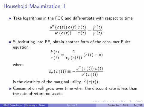
Take logarithms in the FOC and differentiate with respect to time

u′′ (c (t)) c (t)u′ (c (t))

c (t)c (t)

=µ (t)µ (t)

.

Substituting into EE, obtain another form of the consumer Eulerequation:

c (t)c (t)

=1

εu (c(t))(r (t)− ρ)

where

εu (c (t)) ≡ −u′′ (c (t)) c (t)u′ (c (t))

is the elasticity of the marginal utility u′ (c(t)).

Consumption will grow over time when the discount rate is less thanthe rate of return on assets.


Household Maximization III

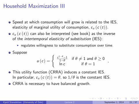
Speed at which consumption will grow is related to the IES,elasticity of marginal utility of consumption, εu (c (t)).

εu (c (t)) can also be interpreted (see book) as the inverseof the intertemporal elasticity of substitution (IES):

I regulates willingness to substitute consumption over time.

Suppose

u (c) =

{c1−θ−11−θ if θ 6= 1 and θ ≥ 0ln c if θ = 1

,

This utility function (CRRA) induces a constant IES.In particular, εu (c (t)) = θ, so 1/θ is the constant IES.

CRRA is necessary to have balanced growth.


Household Maximization IV

Under CRRA utility,µ (t) = c (t)−θ

and the consumer Euler equation yields:

µ (t)µ (t)

= − (r (t)− ρ) = −θc (t)c (t)

=⇒ c (t)c (t)

=r (t)− ρ

θ

Thus, integrating,

µ (t) = µ (0) exp(−∫ t

0(r (s)− ρ) ds

),


Household Maximization V

Consider the TVC

0 = limt→∞

[exp (− (ρ− n) t) · a (t) · µ (t)]

= limt→∞

[exp (− (ρ− n) t) · a (t) · µ (0) exp

(−∫ t

0(r (s)− ρ) ds

)]

= limt→∞

[a (t) exp

(−∫ t

0(r (s)− n) ds

)]· c (0)−θ .

Thus, limt→∞

[a (t) exp

(−∫ t0 (r (s)− n) ds

)]= 0

We can now provide an interpretation of the TVC


Transversality Condition I

The transversality condition is a complementary condition that musthold (in standard problems) in order for the consumption/savingsplan of the individual agents to be optimal.

In a finite-horizon problem,the TVC has a straightforward interpretation:the discounted value of the stock of capital leftat the end of the planning period (T ) must be zero

a (T ) · e−∫ T0 (r (ν)−n) dν = 0

As long as the interest rate is finite, the second term is positive,which reduces itself to the intuitive condition that aT = 0.


Transversality Condition II

In the infinite horizon, we take the limit ofthe finite-horizon condition as T tends to infinity:

limT→∞

[a (T ) · e−

∫ T0 (r (ν)−n) dν

]= 0

Interpretation: the PDV of assets at the “end of life” (infinity)must be zero. However, now a (t) needs not converge to zero.

A simple case in which the TVC holds is an economy convergingto a steady-state where both a (t) and r (t) are constant

However, the TVC can also hold if a (t)→ ∞as long as the second term goes to zero "suffi ciently fast"


Equilibrium Prices IEquilibrium prices are given by

R (t) = f ′ (k(t)) and w (t) = f (k (t))− k (t) f ′ (k(t)).Since r (t) = R (t)− δ, then

r (t) = f ′ (k (t))− δ.

Substituting this into the consumer’s EE, we have

c (t)c (t)

=f ′ (k (t))− δ− ρ

θ

Moreover, since a (t) = k (t) and µ (t) = c (t)−θ , the TVC can bewritten as

limt→∞

[exp (− (ρ− n) t) · µ (t) · a (t)] =

limt→∞

[exp (− (ρ− n) t) · c (t)−θ · k (t)

]= 0


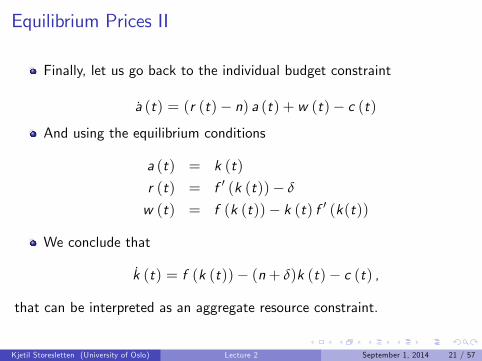
Equilibrium Prices II

Finally, let us go back to the individual budget constraint

a (t) = (r (t)− n) a (t) + w (t)− c (t)And using the equilibrium conditions

a (t) = k (t)

r (t) = f ′ (k (t))− δ

w (t) = f (k (t))− k (t) f ′ (k(t))

We conclude that

k (t) = f (k (t))− (n+ δ)k (t)− c (t) ,

that can be interpreted as an aggregate resource constraint.


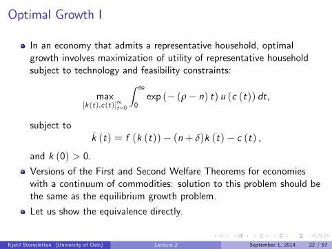
Optimal Growth I

In an economy that admits a representative household, optimalgrowth involves maximization of utility of representative householdsubject to technology and feasibility constraints:

max[k (t),c (t)]∞t=0

∫ ∞

0exp (− (ρ− n) t) u (c (t)) dt,

subject tok (t) = f (k (t))− (n+ δ)k (t)− c (t) ,

and k (0) > 0.

Versions of the First and Second Welfare Theorems for economieswith a continuum of commodities: solution to this problem should bethe same as the equilibrium growth problem.

Let us show the equivalence directly.


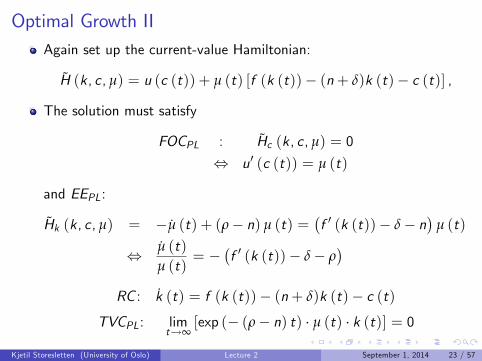
Optimal Growth IIAgain set up the current-value Hamiltonian:

H (k , c, µ) = u (c (t)) + µ (t) [f (k (t))− (n+ δ)k (t)− c (t)] ,

The solution must satisfy

FOCPL : Hc (k, c, µ) = 0

⇔ u′ (c (t)) = µ (t)

and EEPL:

Hk (k, c , µ) = −µ (t) + (ρ− n) µ (t) =(f ′ (k (t))− δ− n

)µ (t)

⇔ µ (t)µ (t)

= −(f ′ (k (t))− δ− ρ

)RC : k (t) = f (k (t))− (n+ δ)k (t)− c (t)

TVCPL: limt→∞

[exp (− (ρ− n) t) · µ (t) · k (t)] = 0


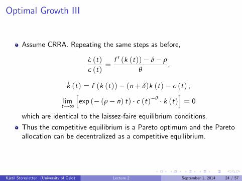
Optimal Growth III

Assume CRRA. Repeating the same steps as before,

c (t)c (t)

=f ′ (k (t))− δ− ρ

θ,

k (t) = f (k (t))− (n+ δ)k (t)− c (t) ,

limt→∞

[exp (− (ρ− n) t) · c (t)−θ · k (t)

]= 0

which are identical to the laissez-faire equilibrium conditions.

Thus the competitive equilibrium is a Pareto optimum and the Paretoallocation can be decentralized as a competitive equilibrium.


Steady-State Equilibrium I

Steady-state equilibrium is defined as an equilibrium path in whichcapital-labor ratio, consumption and output are constant. Thus:

c (t)c (t)

=f ′ (k∗)− δ− ρ

θ= 0

⇐⇒ f ′ (k∗) = ρ+ δ

Pins down the steady-state capital-labor ratio only as a function ofthe production function, the discount rate and the depreciation rate.

Then, the resource constraint pins down the steady-stateconsumption level:

k (t) = f (k (t))− (n+ δ)k (t)− c (t) = 0

⇐⇒ c∗ = f (k∗)− (n+ δ) k∗.


Steady-State Equilibrium II

A steady state where the capital-labor ratio and thus output areconstant necessarily satisfies the TVC:

limt→∞

[exp (− (ρ− n) t) · k∗ · (c∗)−θ

]= 0

which is true as long as ρ > n.


Transitional Dynamics I

Equilibrium is determined by two differential equations:

k (t) = f (k (t))− (n+ δ)k (t)− c (t)

c (t)c (t)

=f ′ (k (t))− δ− ρ

θ

plus an initial condition, k (0) > 0, and a terminal condition:

limt→∞

[exp (− (ρ− n) t) · k (t) · (c (t))−θ

]= 0.


Transitional Dynamics II

Appropriate notion of saddle-path stability:I c (or, equivalently, µ) is the control variable, and c (0) (or µ (0)) isfree: it has to adjust to satisfy transversality condition

I If there were more than one path equilibrium would be indeterminate.

Economic forces are such that indeed there will be a one-dimensionalmanifold of stable solutions tending to the unique steady state.

See Figure.


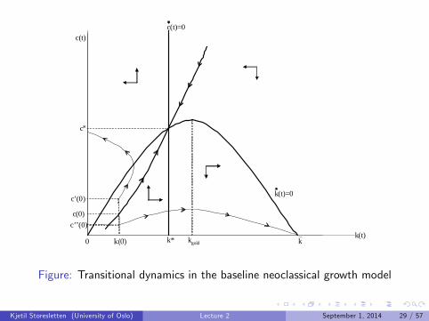
c(t)

kgold0k(t)

k(0)

c’(0)

c’’(0)

c(t)=0

k(t)=0

k*

c(0)

c*

k

Figure: Transitional dynamics in the baseline neoclassical growth model


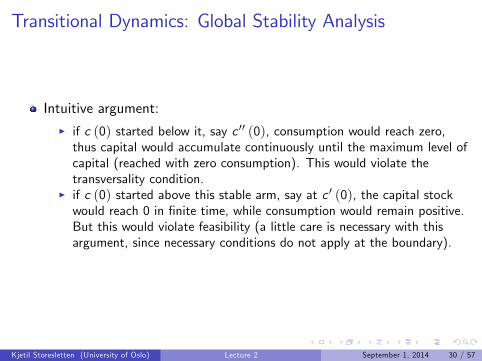
Transitional Dynamics: Global Stability Analysis

Intuitive argument:I if c (0) started below it, say c ′′ (0), consumption would reach zero,thus capital would accumulate continuously until the maximum level ofcapital (reached with zero consumption). This would violate thetransversality condition.

I if c (0) started above this stable arm, say at c ′ (0), the capital stockwould reach 0 in finite time, while consumption would remain positive.But this would violate feasibility (a little care is necessary with thisargument, since necessary conditions do not apply at the boundary).


Technological Change and the Canonical NeoclassicalModel I

Extend the production function to:

Y (t) = F [K (t) ,A (t) L (t)] ,

whereA (t) = exp (gt)A (0) .

Note: we assume labor-augmenting technological change.Else, there would be no balanced growth equilibrium


Technological Change and the Canonical NeoclassicalModel II

Define x (t) ≡ X (t) / (A (t) L (t))

y (t) = F[

K (t)A (t) L (t)

, 1]≡ f

(k (t)

),

Assume CRRA preferences


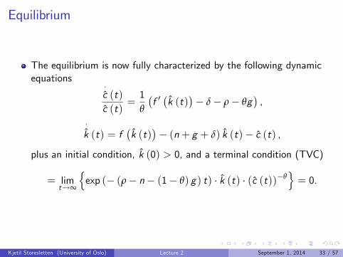
Equilibrium

The equilibrium is now fully characterized by the following dynamicequations

·c (t)c (t)

=1θ

(f ′(k (t)

)− δ− ρ− θg

),

·k (t) = f

(k (t)

)− (n+ g + δ) k (t)− c (t) ,

plus an initial condition, k (0) > 0, and a terminal condition (TVC)

= limt→∞

{exp (− (ρ− n− (1− θ) g) t) · k (t) · (c (t))−θ

}= 0.


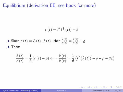
Equilibrium (derivation EE, see book for more)

r (t) = f ′(k (t)

)− δ

Since c (t) = A (t) · c (t) , then·c (t)c (t) =

·c (t)c (t) + g

Then:

·c (t)c (t)

=1θ(r (t)− ρ)⇐⇒

·c (t)c (t)

=1θ

(f ′(k (t)

)− δ− ρ− θg

)


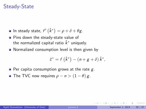
Steady-State

In steady state, f ′(k∗)= ρ+ δ+ θg .

Pins down the steady-state value ofthe normalized capital ratio k∗ uniquely.

Normalized consumption level is then given by

c∗ = f(k∗)− (n+ g + δ) k∗,

Per capita consumption grows at the rate g .

The TVC now requires ρ− n > (1− θ) g .


Technological Change and the Canonical NeoclassicalModel XI

Proposition Consider the neoclassical growth model with laboraugmenting technological progress at the rate g and CRRApreferences. Suppose that ρ− n > (1− θ) g . Then thereexists a unique balanced growth path with a normalizedcapital to effective labor ratio of k∗, given byf ′(k∗)= ρ+ δ+ θg , and output per capita and

consumption per capita grow at the rate g .


Transitional dynamics

c(t)

kgold0k(t)

k(0)

c’(0)

c’’(0)

c(t)=0

k(t)=0

k*

c(0)

c*

k

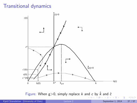
Figure: When g>0, simply replace k and c by k and c


Comparative Dynamics I

Comparative statics: changes in steady state in response to changesin parameters.

Comparative dynamics look at how the entire equilibrium path ofvariables changes in response to a change in policy or parameters.

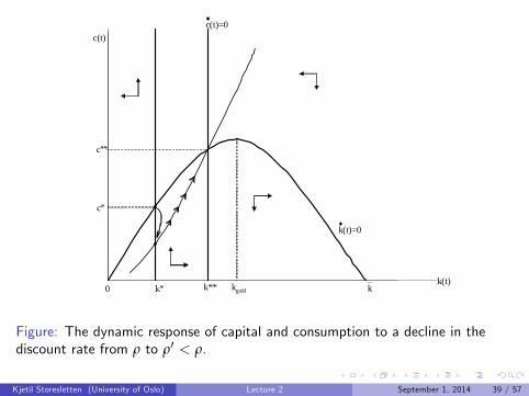
E.g.: Initial steady state represented by (k∗, c∗). Unexpectedly,discount rate declines to ρ′ < ρ.

Following the decline c∗ is above the stable arm of the new dynamicsystem: consumption must drop immediately


c(t)

kgold0k(t)

k*

c(t)=0

k(t)=0

k**

c**

c*

k

Figure: The dynamic response of capital and consumption to a decline in thediscount rate from ρ to ρ′ < ρ.


The Role of Policy I

Introduce linear tax policy: returns on capital net of depreciation aretaxed at the rate τ and the proceeds of this are redistributed back tothe consumers.

Capital accumulation equation remains as above:

·k (t) = f

(k (t)

)− c (t)− (n+ g + δ) k (t) ,

But interest rate faced by households changes to:

r (t) = (1− τ)(f ′(k (t)

)− δ),


The Role of Policy II

Growth rate of normalized consumption is then obtained from theconsumer Euler equation

·c (t)c (t)

=1θ(r (t)− ρ− θg) .

=1θ

((1− τ)

(f ′(k (t)

)− δ)− ρ− θg

).

This implies

f ′(k∗)= δ+

ρ+ θg1− τ

.

Since f ′ (·) is decreasing, higher τ, reduces k∗.

Higher taxes on capital have the effect of depressing capitalaccumulation and reducing income per capita.


Appraisal neoclassical model

Major contribution: open the black box of capital accumulation byspecifying the preferences of consumers.

Also by specifying individual preferences we can explicitly compareequilibrium and optimal growth.

Paves the way for further analysis of capital accumulation, humancapital and endogenous technological progress.

However, this model, by itself, does not enable us to answer questionsabout the fundamental causes of economic growth.

But it clarifies the nature of the economic decisions so that we are ina better position to ask such questions.


AK model I

Neoclassical model: no autonomous engine of growth. In the absenceof exogenous trend, growth dies off in the long-run.

1 No theory of determinants of long-run growth;2 No theory of determinants of long-run cross-country differences ingrowth rates;

3 Policies do not affect long-run growth.

The AK-Model is a very simple model that can be viewed as the "limitcase" of the neoclassical growth model. It provides the commonanalytical framework for a number of more interesting applications.


AK model II

Production technology (g=0):

f (k) = Ak

Equilibrium interest rate is r (t) = A− δ.

Assume CRRA utility

Given k (0) , a competitive equilibrium is determined by

c (t) =A− δ− ρ

θ· c (t) (EE)

k (t) = Ak (t)− c (t)− (δ+ n) k (t) (BC)

limt→∞

[exp (− (ρ− n) t) · k (t) · (c (t))−θ

]= 0 (TVC)


AK model IIIWe can obtain an explicit analytical solution:

(a) Guess a steady-state solution such that c/k is constant(assume A > δ+ ρ).

c (t)c (t)

=k (t)k (t)

=A− δ− ρ

θ= γ

(b) Use (BC)

k (t)k (t)

= (A− δ− n)− c (t)k (t)

.

(c) From (a)+(b):

c (t)k (t)

=ck= ρ− n− 1− θ

θ· [A− δ− ρ]

In particular:c (0) =

{ρ− n− 1−θ

θ · [A− δ− ρ]}k (0) .


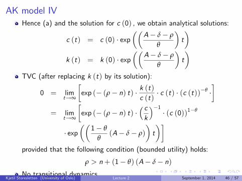
AK model IVHence (a) and the solution for c (0) , we obtain analytical solutions:

c (t) = c (0) · exp((

A− δ− ρ

θ

)t)

k (t) = k (0) · exp((

A− δ− ρ

θ

)t)

TVC (after replacing k (t) by its solution):

0 = limt→∞

[exp (− (ρ− n) t) · k (t)

c (t)· c (t) · (c (t))−θ ·

]= lim

t→∞

[exp (− (ρ− n) t) ·

( ck

)−1· (c (0))1−θ

· exp((

1− θ

θ(A− δ− ρ)

)t)]

provided that the following condition (bounded utility) holds:

ρ > n+ (1− θ) (A− δ− n)No transitional dynamics.


AK model V

In this model, policies have permanent effects on growth.

Consider again the introduction of a permanent tax on the returns oncapital. The proceeds are rebated as lump-sums.

The equilibrium interest rate is r = (1− τ) (A− δ), and theequilibrium growth rate is:

γτ =(1− τ) (A− δ)− ρ

θ


Two Simple AK Models

Two simple models that deliver AK dynamics

Assume n=g=0

Basic human capital and knowledge spillovers


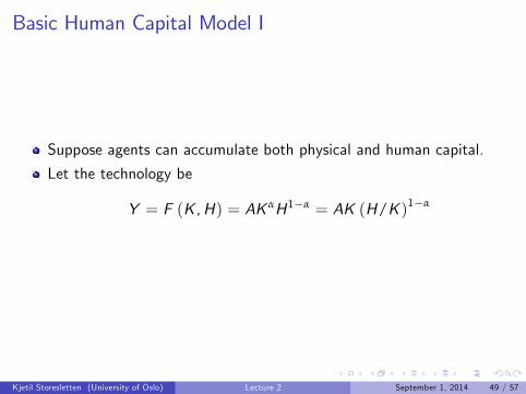
Basic Human Capital Model I

Suppose agents can accumulate both physical and human capital.

Let the technology be

Y = F (K ,H) = AK αH1−α = AK (H/K )1−α


Basic Human Capital Model II

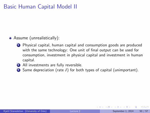
Assume (unrealistically):1 Physical capital, human capital and consumption goods are producedwith the same technology: One unit of final output can be used forconsumption, investment in physical capital and investment in humancapital.

2 All investments are fully reversible.3 Same depreciation (rate δ) for both types of capital (unimportant).


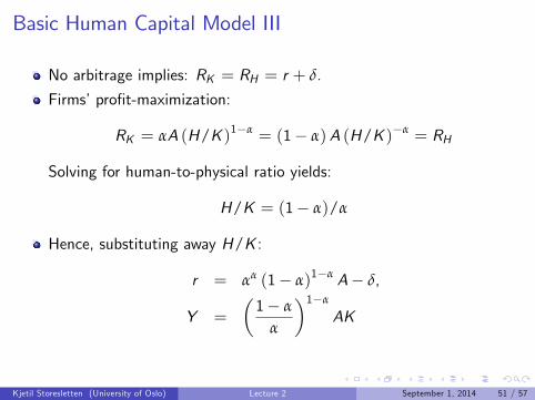
Basic Human Capital Model III

No arbitrage implies: RK = RH = r + δ.

Firms’profit-maximization:

RK = αA (H/K )1−α = (1− α)A (H/K )−α = RH

Solving for human-to-physical ratio yields:

H/K = (1− α)/α

Hence, substituting away H/K :

r = αα (1− α)1−α A− δ,

Y =

(1− α

α

)1−α

AK


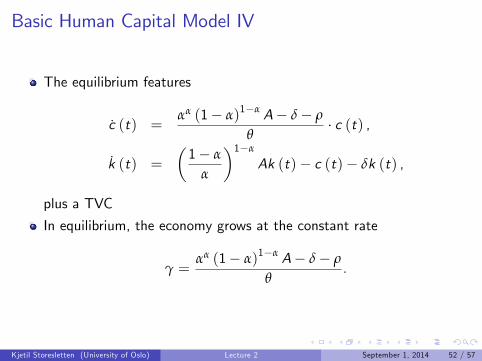
Basic Human Capital Model IV

The equilibrium features

c (t) =αα (1− α)1−α A− δ− ρ

θ· c (t) ,

k (t) =

(1− α

α

)1−α

Ak (t)− c (t)− δk (t) ,

plus a TVC

In equilibrium, the economy grows at the constant rate

γ =αα (1− α)1−α A− δ− ρ

θ.


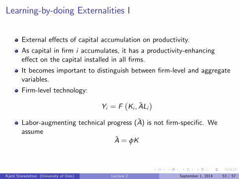
Learning-by-doing Externalities I

External effects of capital accumulation on productivity.

As capital in firm i accumulates, it has a productivity-enhancingeffect on the capital installed in all firms.

It becomes important to distinguish between firm-level and aggregatevariables.

Firm-level technology:

Yi = F(Ki , ALi

)Labor-augmenting technical progress (A) is not firm-specific. Weassume

A = φK


Learning-by-doing Externalities II

A can be interpreted as public knowledge. Knowledge is assumed tohave a non-rival character: when a firm adds to the stock ofknowledge, all firms in the economy can benefit from this addition.

Knowledge accumulation is assumed to be a pure spillover.

For simplicity, we restrict attention to Cobb-Douglas technology:

F(Ki , ALi

)= K α

i

(ALi)1−α

= AK αi (KLi )

1−α

where A ≡ φ1−α


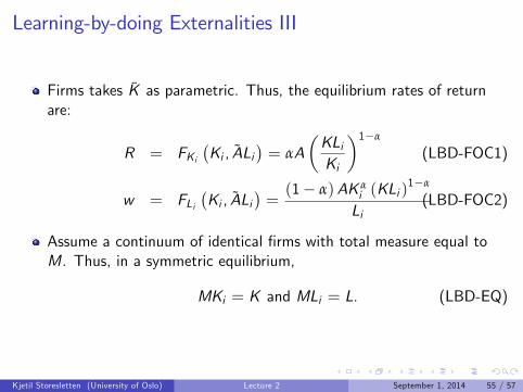
Learning-by-doing Externalities III

Firms takes K as parametric. Thus, the equilibrium rates of returnare:

R = FKi(Ki , ALi

)= αA

(KLiKi

)1−α

(LBD-FOC1)

w = FLi(Ki , ALi

)=(1− α)AK α

i (KLi )1−α

Li(LBD-FOC2)

Assume a continuum of identical firms with total measure equal toM. Thus, in a symmetric equilibrium,

MKi = K and MLi = L. (LBD-EQ)


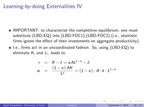
Learning-by-doing Externalities IV

IMPORTANT: to characterize the competitive equilibrium, one mustsubstitute (LBD-EQ) into (LBD-FOC1)-(LBD-FOC2) (i.e., atomisticfirms ignore the effect of their investments on aggregate productivity).

I.e., firms act in an uncoordinated fashion. So, using (LBD-EQ) toeliminate Ki and Li , leads to:

r = R − δ = αAL1−α − δ

w =(1− α)AK

Lα= (1− α) · A · k · L1−α


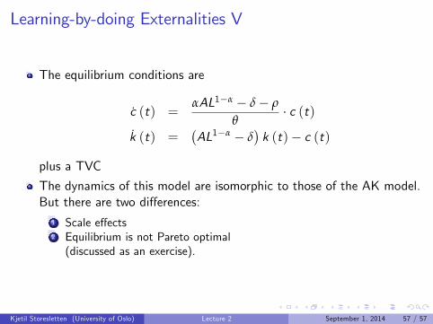
Learning-by-doing Externalities V

The equilibrium conditions are

c (t) =αAL1−α − δ− ρ

θ· c (t)

k (t) =(AL1−α − δ

)k (t)− c (t)

plus a TVC

The dynamics of this model are isomorphic to those of the AK model.But there are two differences:

1 Scale effects2 Equilibrium is not Pareto optimal(discussed as an exercise).


lecture 2: neoclassical growth theory acemoglu …lecture 2: neoclassical growth theory (acemoglu...

Documents