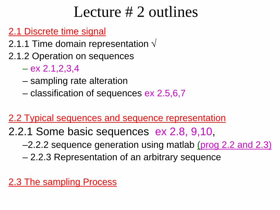
Lecture # 2 outlines2.1 Discrete time signal2.1.1 Time domain representation √2.1.2 Operation on sequences

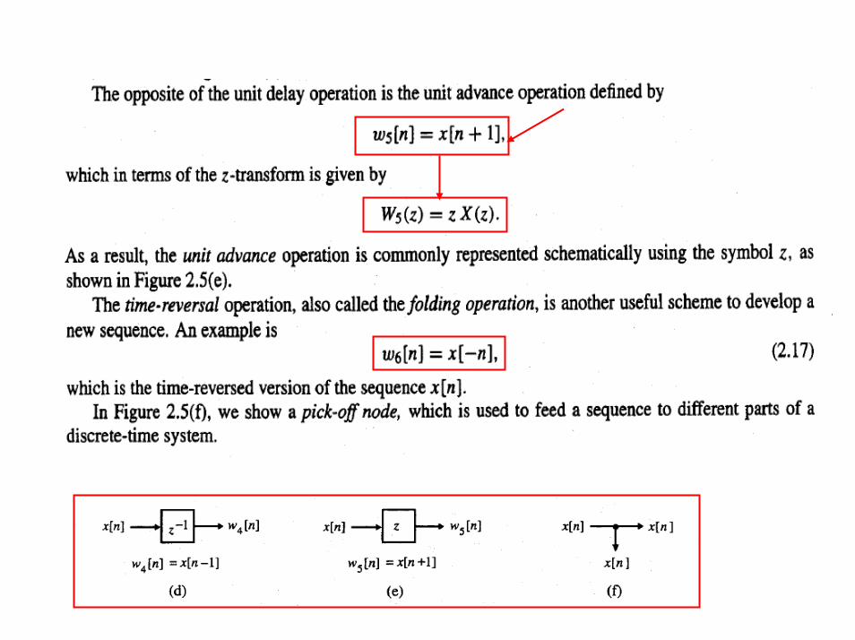
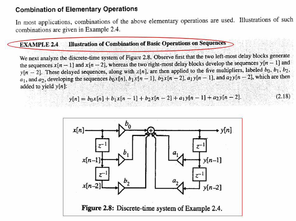
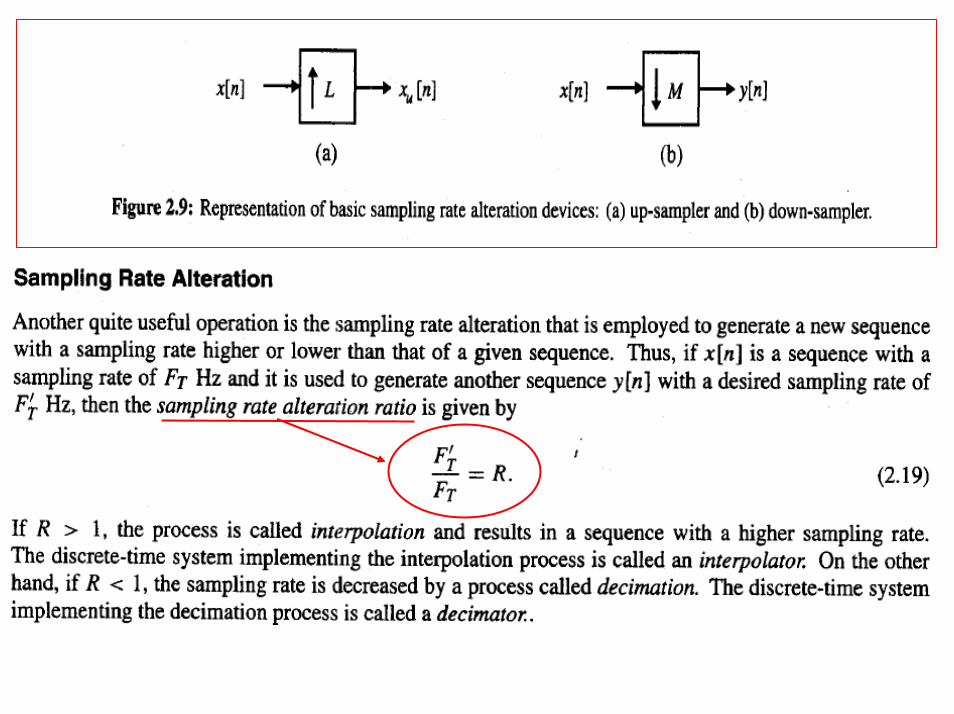
– ex 2.1,2,3,4– sampling rate alteration– classification of sequences ex 2.5,6,7

2.2 Typical sequences and sequence representation2.2.1 Some basic sequences ex 2.8, 9,10,

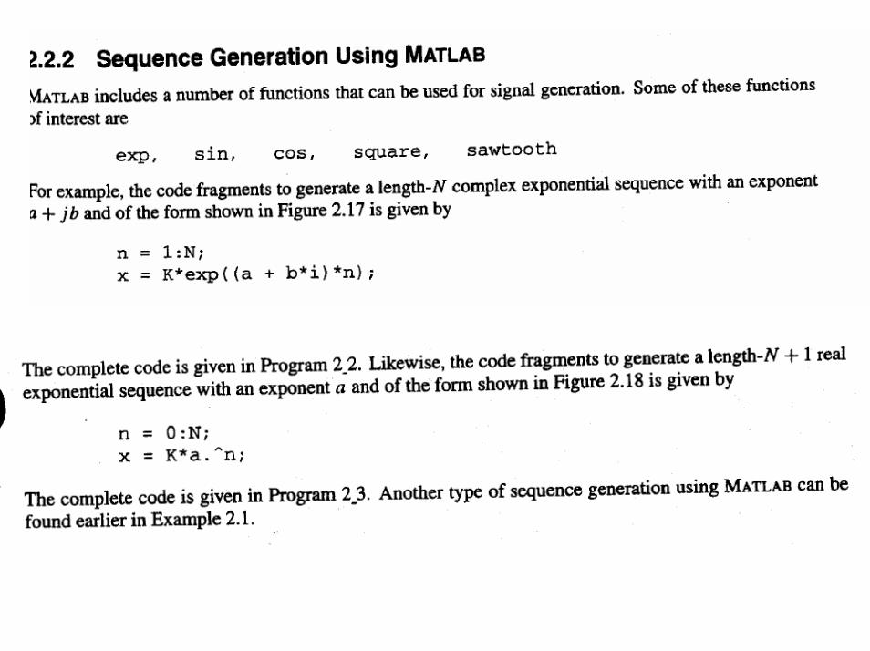
–2.2.2 sequence generation using matlab (prog 2.2 and 2.3)– 2.2.3 Representation of an arbitrary sequence

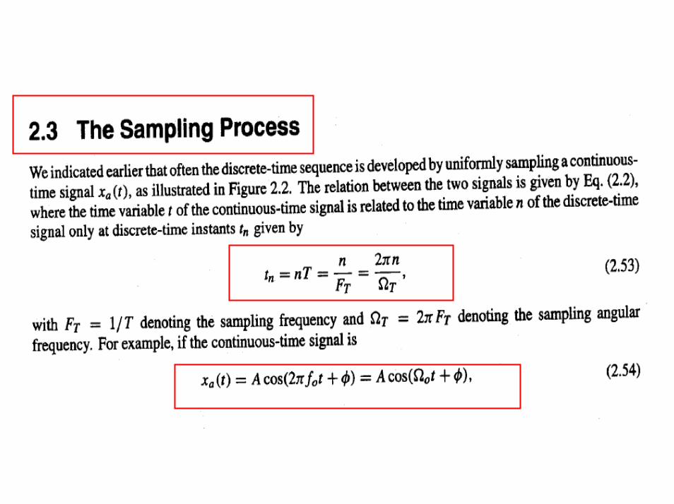
2.3 The sampling Process

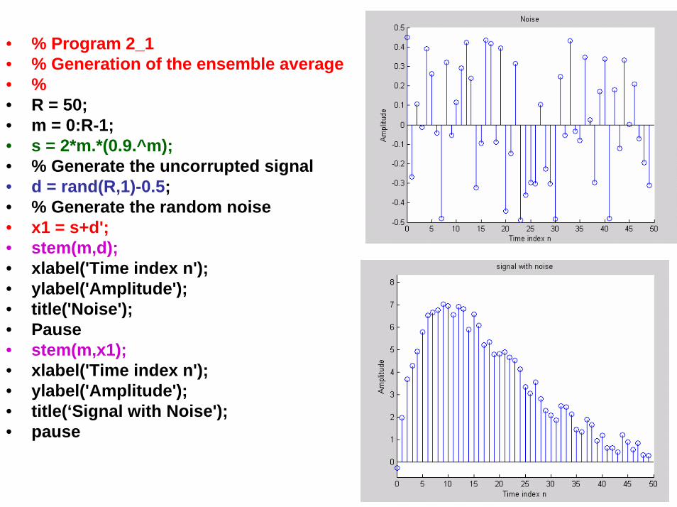
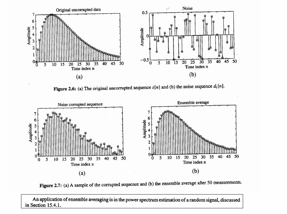
• % Program 2_1• % Generation of the ensemble average• %• R = 50;• m = 0:R-1;• s = 2*m.*(0.9.^m);• % Generate the uncorrupted signal• d = rand(R,1)-0.5; • % Generate the random noise• x1 = s+d';• stem(m,d);• xlabel('Time index n');• ylabel('Amplitude');• title('Noise');• Pause• stem(m,x1);• xlabel('Time index n');• ylabel('Amplitude');• title(‘Signal with Noise');• pause

• for n = 1:50;• d = rand(R,1)-0.5;• x = s + d';• x1 = x1 + x;• end• x1 = x1/50;• stem(m,x1);• xlabel('Time index n');• ylabel('Amplitude');• title('Ensemble average');

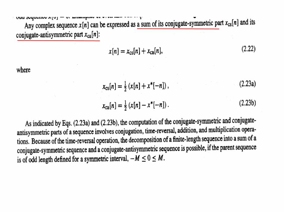
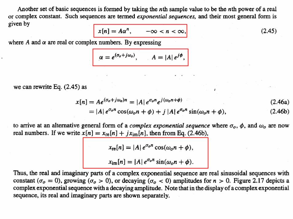
Consider the finite length sequence

{g[n]}={0, 1+j4, -2+j3, 4-j2, -5-j6, -j2, 3}

Find its conjugate symmetric part and its conjugate antisymmetric part

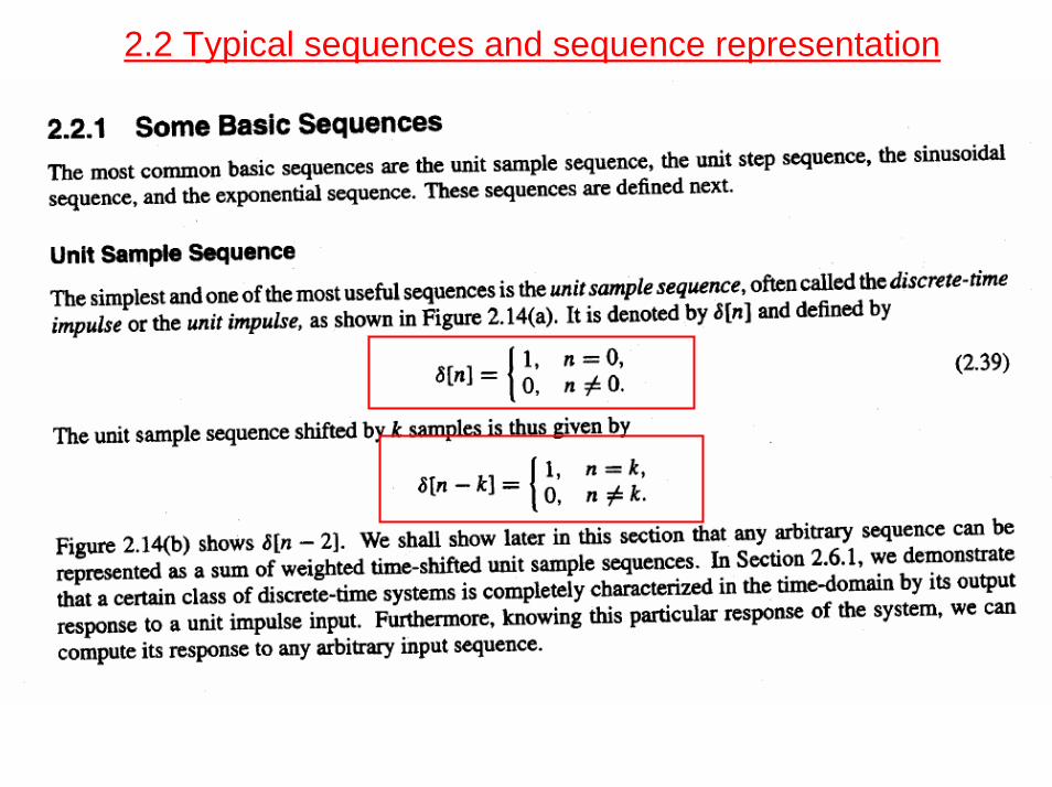
2.2 Typical sequences and sequence representation

Assignment (1)

Matlab Exercises

Example 2.8: Determination of the period of sinusoidal sequence

Example 2.9: Generation of a sequence wave sequenceAssignment (2)

page 115, M2.1,3,4

Due date next Thursday 1/27

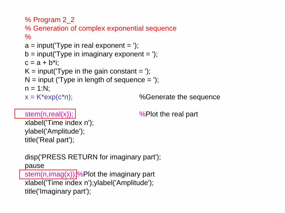
% Program 2_2% Generation of complex exponential sequence%a = input('Type in real exponent = ');b = input('Type in imaginary exponent = ');c = a + b*i;K = input('Type in the gain constant = ');N = input ('Type in length of sequence = ');n = 1:N;x = K*exp(c*n); %Generate the sequence

stem(n,real(x)); %Plot the real partxlabel('Time index n');ylabel('Amplitude');title('Real part');

disp('PRESS RETURN for imaginary part');pausestem(n,imag(x));%Plot the imaginary partxlabel('Time index n');ylabel('Amplitude');title('Imaginary part');

• % Program 2_3• % Generation of real exponential sequence• %• a = input('Type in argument = ');• K = input('Type in the gain constant = ');• N = input ('Type in length of sequence = ');• n = 0:N;• x = K*a.^n;• stem(n,x);• xlabel('Time index n');ylabel('Amplitude');• title(['\alpha = ',num2str(a)]);

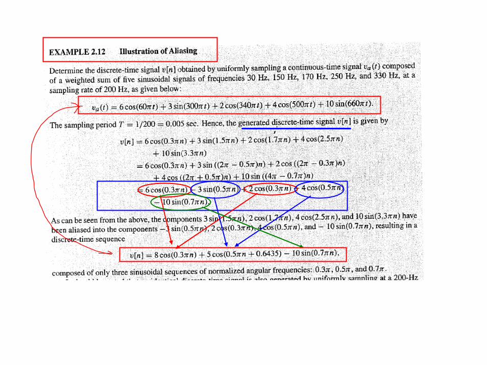
See Example 2.11

the solid line describes a 0.5Hz continuous-time sinusoidal signal and the dash-dot line describes a 1.5 Hz continuous time sinusoidal signal.

When both signals are sampled at the rate of Fs equals two samples/sec, their samples coincide, as indicated by the circles in the figures. This means that x one of n (T sub s) is equal to x two of n (T sub s) and there is no way to distinguish the two signals apart from their sampled versions.

This phenomenon, known as aliasing, occurs whenever F2 plus or minus F1 is a multiple of the sampling rate

Frequency = 3, 7, 13 Hz, sampling rate = 10 Hz with T=0.1 secg1[n]=cos(0.6 .pi. n), g2[n]=cos(1.4 .pi. n), g3[n]=cos(2.6 .pi. n)

As a result all three sequences above are identical and it is difficult to Associate a unique continuous time function with any one of these sequences

Matlab Aliasing demoAliasing Demo (1)

The phenomenon of aliasing happens when the sampling frequency is less than twice the highest frequency of band-limited input signal.

In this example, the input signal is a sinusoidal signal of frequency 1.8KHz.

Three output sound signals are generated in sampling rates 8KHz, 4KHz and 2.6667KHz respectively.

Among these three outputs, we can observe that the aliasing arises only at sampling frequency of 2.6667KHz, which is less than twice of the highest input frequency 3.6KHz.

MATLAB file: aliasing.m