Lecture 21: Compartment Models

36-467/36-667

15 November 2018

Abstract

“Compartment models”, which track the transitions of large numbers of in-dividuals across a series of qualitatively-distinct states (the “compartments”) arecommon in fields which study large populations, such as epidemiology and so-ciology. These notes cover such models as a particular kind of Markov chain,including some examples from epidemiology, evolutionary economics, and de-mography.

I made some mistakes in lecture; these notes correct them.

Epidemiology, ecology, sociology, demography, chemical kinetics, and some otherfields are sometimes grouped together as “population sciences”, which study the be-havior and evolution of large populations of individuals. All of these fields makeextensive use of what are called (among other things) “compartment models”, wherethe members of the population are divided into a discrete set of qualitatively-distinctstates (or “compartments”), and transition between them at rates which vary as func-tions of the current distribution over compartments1. They can be used whenever apopulation is divided into discrete, qualitatively-distinct types or classes, and transi-tions between classes are stochastic.

1 Compartment Models in General

1.1 Basic Definitions and AssumptionsLet’s begin with the case of a “closed” population of constant size n. (§5 will considerthe modifications needed to make the population size vary over time.) This popula-tion is divided into r ≥ 2 qualitatively distinct classes, types or compartments2, andwe are primarily interested in how many individuals are located in each compartment.We thus define the state of the population at time t , X (t ), as a vector,

X (t )≡ [X1(t ),X2(t ), . . .Xr (t )] (1)

where Xi (t ) counts how many individuals are in compartment i at time t .

1Whether the ubiquity of these models reflects some underlying commonality across these fields, or justa tendency for scientists with similar mathematical training to borrow and/or re-invent similar models, isbeyond the scope of this note.

2These words are all synonyms in the present context.

1

The state X (t ) changes because individuals can move from one compartment toanother. We assume that these moves or transitions follow a stochastic process, andwe make two important assumptions about that process.

1. The i -to- j transition rate pi j is the probability that an individual in compart-ment i will move to compartment j at the next time step. ( pi i is thus the prob-ability of staying in compartment i .) We assume that the transition rates arefunctions of the current population state, and not the past (or the future), sopi j (X ) is a well-defined function.

Note that this assumption allows some pi j to be zero, either always or for cer-tain states of the population. (These are sometimes called forbidden or sup-pressed transitions.) It also allows some pi j to be constant, regardless of X .

2. All individuals in the population make independent transitions, conditional onX (t ). The moves of all the individuals in a given compartment are thus condi-tionally independent and identically distributed.

These assumptions are not implied by the mere fact that we’ve divided the pop-ulation into compartments and are tracking the number of individuals in each com-partment. They could be false, or true only for a different choice of compartments,etc.

— You may feel some scruples about applying these assumptions to people, atleast to social processes which reflect human actions (as opposed to, say, models ofdisease spread). But modeling aggregated social processes as stochastic in this waydoes not commit us to saying that people act randomly, or don’t have motives fortheir actions, or that all individuals in the same compartment are identical. What itdoes commit us to is that the differences between people in the same compartmentwhich determine their motives and their actions are so various, so complicated, andso independent of the circumstances which landed them in that compartment thatthey can’t be predicted, and can be effectively treated as random3.

1.2 Consequences of the AssumptionsThese assumptions are enough to tell us that the sequence of random variables X (t ) isa Markov chain. If it’s a Markov process, it has to be a Markov chain because the statespace is discrete, though large (Exercise 1), so what we really need to do is show thatthe Markov property holds. The easiest way to get there is through defining someadditional variables.

3There are precise technical senses in which any sufficiently complicated function is indistinguishablefrom randomness. For a brilliant and accessible introduction to these ideas, and how they underlie prob-ability modeling, I strongly recommend Ruelle (1991). The standard textbook on this subject is Li andVitányi (1997). Salmon (1984, ch. 3) applies these ideas to the problem of defining “the” probability of anoutcome for members of some class.

2

1.2.1 Flow or Flux Variables

For each pair of compartments i and j , define Yi j (t+1) as the number of individualswho moved from compartment i to compartment j at time t + 1. This is sometimescalled the flow or flux from i to j .

Yi j (t+1) is a random quantity. By the assumptions above, in fact, it has a binomialdistribution:

Yi j (t + 1)∼ Binom(Xi (t ), pi j (X (t ))) (2)

This implies that

E�

Yi j (t + 1)|X (t )�

= Xi (t )pi j (X (t )) (3)

Var�

Yi j (t + 1)|X (t )�

= Xi (t )pi j (X (t ))(1− pi j (X (t ))) (4)

There are two implications of these worth noting.

1. Both the expected flux and the variance in the flux are proportional to Xi (t ).This means that the standard deviation in the flux is only proportional to

p

Xi .Thus, if Xi (t ) is large, the relative deviations in the flux are shrinking. Thissuggests that there should be nearly-deterministic behavior in large populations.

2. The assumption that each individual in compartment i has the same probabilityof moving to compartment j is crucial to calculating the variance. If there wererandomly-distributed transition rates for all individuals in the compartment,we’d see a higher variance for the flux (Exercise 2).

If r > 2, then the set of fluxes out of i , [Yi1(t +1),Yi2(t +1), . . .Yi r (t +1)] has asits joint distribution a multinomial, with the number of “trials” being Xi (t ), and theprobabilities being (pi1, pi2, . . . pi r ). (Remember that the marginal distributions of amultinomial distribution are binomial.)

1.2.2 Stock-Flow Consistency

The variables Xi (t ) count the total number of individuals in each compartment, re-gardless of how or when they arrived there. Such variables are sometimes called stockor level variables. The Yi j (t ) variables, on the other hand, are (as already said) flowor flux variables. A basic principle is that the new level of the stock is the old level,plus flows in, minus flows out:

Xi (t + 1) = Xi (t )+∑

j 6=i

Yi j (t + 1)−Y j i (t + 1) (5)

(new level) = (old level)+∑

(in flow)− (out flow) (6)

This is sometimes called stock-flow consistency.

3

1.2.3 Markov Property

Because Eq. 5 says how the level in each compartment changes, it tells us how the statevector X (t ) changes as well.

Notice that, from our assumptions, Yi j (t + 1) is independent of the past givenX (t ). It is independent of earlier values of X , and also independent of earlier valuesof the Y ’s. Since Eq. 5 tells us that X (t + 1) is a deterministic function of X (t ) andY (t + 1), it follows that X (t + 1) is independent of earlier X ’s (and Y ’s) given X (t ).Hence the state of the population follows a Markov chain.

Because the state space, while large, is finite, the Markov chain will eventuallyenter some closed, irreducible set, and stay there forever. In the long run, the distri-bution of X (t ) will follow the invariant distribution for that irreducible set. Theseare properties of any finite Markov chain, and so apply to this one, even though itshas special structure.

2 Epidemic ModelsIn epidemiology, compartment models are often known as “epidemic models”, andin that field they descend from pioneering work in mathematical epidemiology donein the early 20th century4, but they are applied much more broadly than just to epi-demics. It’s worth thinking through some of the most basic cases, to get a feel for howthey work.

2.1 SILet’s begin with a model with just two compartments, dividing the entire populationinto those who are infected with a certain disease — call this compartment I — andthose who, not having caught the disease yet, are susceptible, in compartment S. Thestate of the population is X (t ) = (XI (t ),XS (t )), but since XS (t ) = n − XI (t ), it isenough to keep track of XI (t ).

With two compartments, we need to specify two rates, pSI and pI S . The former isthe rate at which susceptible individuals become infected; the later is the rate at whichinfected individuals are cured and become susceptible again.

A simple assumption is that pSI (XS ,XI ) = αXI , because the more members of thepopulation are infected, the more likely a susceptible individual is to encounter oneand become infected. We might, however, simply set pI S = 0, indicating that no onerecovers from the disease, but rather the infected remain infected, and contagious,forever. There are a couple of ways to justify this latter assumption.

1. We’re in a zombie movie. (This is Pittsburgh, after all.)

2. We’re only interested in what happens on a comparatively short time scale.More precisely, whatever processes make infected individuals non-infectious(recovery, death, quarantine, etc.) happen much more slowly than the process

4It is conventional these days to attribute this to the work of Sir Ronald Ross on malaria, but earlyreviews (e.g., Lotka 1924, ch. VIII, pp. 79–82) make it clear that this was much more of a collective effort.

4

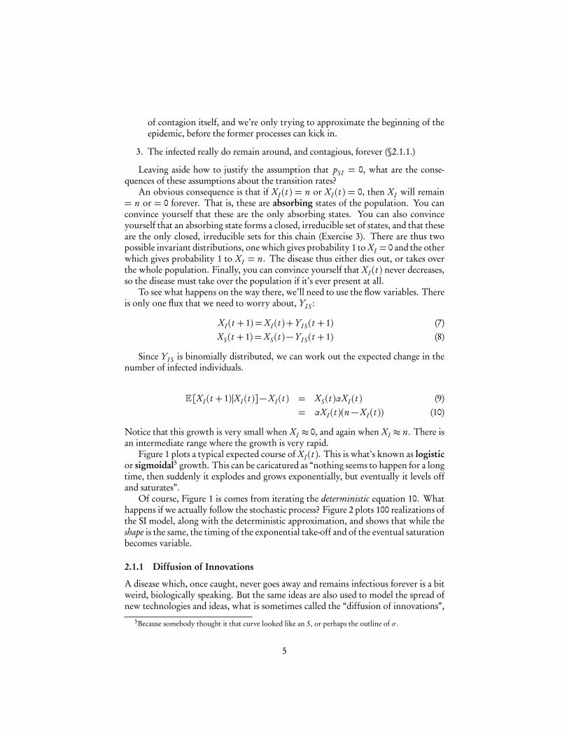
of contagion itself, and we’re only trying to approximate the beginning of theepidemic, before the former processes can kick in.

3. The infected really do remain around, and contagious, forever (§2.1.1.)

Leaving aside how to justify the assumption that pSI = 0, what are the conse-quences of these assumptions about the transition rates?

An obvious consequence is that if XI (t ) = n or XI (t ) = 0, then XI will remain= n or = 0 forever. That is, these are absorbing states of the population. You canconvince yourself that these are the only absorbing states. You can also convinceyourself that an absorbing state forms a closed, irreducible set of states, and that theseare the only closed, irreducible sets for this chain (Exercise 3). There are thus twopossible invariant distributions, one which gives probability 1 to XI = 0 and the otherwhich gives probability 1 to XI = n. The disease thus either dies out, or takes overthe whole population. Finally, you can convince yourself that XI (t ) never decreases,so the disease must take over the population if it’s ever present at all.

To see what happens on the way there, we’ll need to use the flow variables. Thereis only one flux that we need to worry about, YI S :

XI (t + 1) =XI (t )+YI S (t + 1) (7)XS (t + 1) =XS (t )−YI S (t + 1) (8)

Since YI S is binomially distributed, we can work out the expected change in thenumber of infected individuals.

E [XI (t + 1)|XI (t )]−XI (t ) = XS (t )αXI (t ) (9)= αXI (t )(n−XI (t )) (10)

Notice that this growth is very small when XI ≈ 0, and again when XI ≈ n. There isan intermediate range where the growth is very rapid.

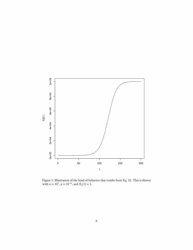
Figure 1 plots a typical expected course of XI (t ). This is what’s known as logisticor sigmoidal5 growth. This can be caricatured as “nothing seems to happen for a longtime, then suddenly it explodes and grows exponentially, but eventually it levels offand saturates”.

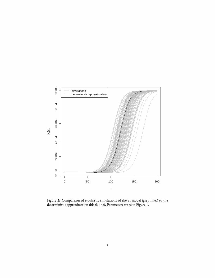
Of course, Figure 1 is comes from iterating the deterministic equation 10. Whathappens if we actually follow the stochastic process? Figure 2 plots 100 realizations ofthe SI model, along with the deterministic approximation, and shows that while theshape is the same, the timing of the exponential take-off and of the eventual saturationbecomes variable.

2.1.1 Diffusion of Innovations

A disease which, once caught, never goes away and remains infectious forever is a bitweird, biologically speaking. But the same ideas are also used to model the spread ofnew technologies and ideas, what is sometimes called the “diffusion of innovations”,

5Because somebody thought it that curve looked like an S, or perhaps the outline of σ .

5

0 50 100 150 200

0e+

002e

+04

4e+

046e

+04

8e+

041e

+05

t

XI(t

)

Figure 1: Illustration of the kind of behavior that results from Eq. 10. This is shownwith n = 105, α= 10−6, and XI (1) = 1.

6

0 50 100 150 200

0e+

002e

+04

4e+

046e

+04

8e+

041e

+05

t

XI(t

)

simulationsdeterministic approximation

Figure 2: Comparison of stochastic simulations of the SI model (grey lines) to thedeterministic approximation (black line). Parameters are as in Figure 1.

7

and then it makes sense to say that those who have “caught” an idea remain infectedwith it, and potentially contagious, for the rest of their lives.

This week’s homework explores this idea in the context of one of the classic data-sets on the diffusion of innovations, about the spread of the use of a new antibioticamong doctors in four towns in Illinois in the 1950s. The same notions, however,have been used to model the adoption of a wide range of technologies, practices, artforms, and ideologies (Rogers, 2003).

It’s worth noting that the idea of analogizing the spread of ideas or behavior to thespread of disease is a very old one, but it’s usually been an analogy deployed when peo-ple disapprove of what is spreading. (It is very rare to talk about “infectious virtue”.)The oldest example I have found is the Roman writer and politician Pliny the Youngercalling Christianity a “contagious superstition” (superstitionis contagio) in a letter tothe Emperor Trajan in +110 (Epistles X 96.9), but the analogy has spontaneously re-curred many, many times since then. It was also the basis for more systematic andscholarly studies, such as Siegfried (1960/1965), long before Dawkins (1976) coinedthe word “meme”.

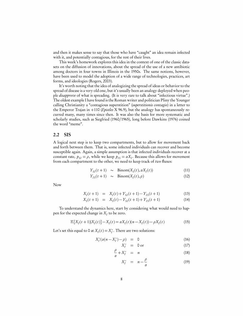
2.2 SISA logical next step is to keep two compartments, but to allow for movement backand forth between them. That is, some infected individuals can recover and becomesusceptible again. Again, a simple assumption is that infected individuals recover at aconstant rate, pSI = ρ, while we keep pI S = αXI . Because this allows for movementfrom each compartment to the other, we need to keep track of two fluxes:

YSI (t + 1) ∼ Binom(XS (t ),αXI (t )) (11)YI S (t + 1) ∼ Binom(XI (t ),ρ) (12)

Now

XI (t + 1) = XI (t )+YSI (t + 1)−YI S (t + 1) (13)XS (t + 1) = XS (t )−YSI (t + 1)+YI S (t + 1) (14)

To understand the dynamics here, start by considering what would need to hap-pen for the expected change in XI to be zero.

E [XI (t + 1)|XI (t )]−XI (t ) = αXI (t )(n−XI (t ))−ρXI (t ) (15)

Let’s set this equal to 0 at XI (t ) =X ∗I . There are two solutions:

X ∗I (α(n−X ∗I )−ρ) = 0 (16)X ∗I = 0 or (17)

ρ

α+X ∗I = n (18)

X ∗I = n−ρ

α(19)

8

0 100 200 300 400

0e+

002e

+04

4e+

046e

+04

8e+

041e

+05

t

XI(t

)

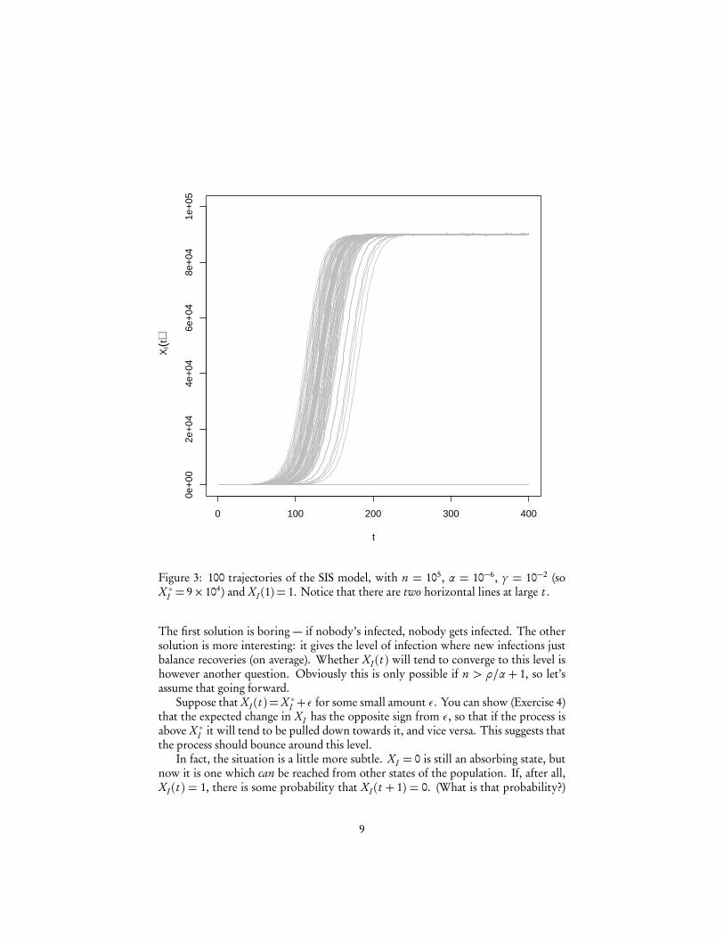
Figure 3: 100 trajectories of the SIS model, with n = 105, α = 10−6, γ = 10−2 (soX ∗I = 9× 104) and XI (1) = 1. Notice that there are two horizontal lines at large t .

The first solution is boring — if nobody’s infected, nobody gets infected. The othersolution is more interesting: it gives the level of infection where new infections justbalance recoveries (on average). Whether XI (t ) will tend to converge to this level ishowever another question. Obviously this is only possible if n > ρ/α+ 1, so let’sassume that going forward.

Suppose that XI (t ) =X ∗I +ε for some small amount ε. You can show (Exercise 4)that the expected change in XI has the opposite sign from ε, so that if the process isabove X ∗I it will tend to be pulled down towards it, and vice versa. This suggests thatthe process should bounce around this level.

In fact, the situation is a little more subtle. XI = 0 is still an absorbing state, butnow it is one which can be reached from other states of the population. If, after all,XI (t ) = 1, there is some probability that XI (t + 1) = 0. (What is that probability?)

9

200 250 300 350 400

8600

088

000

9000

092

000

9400

0

t

XI(t

)

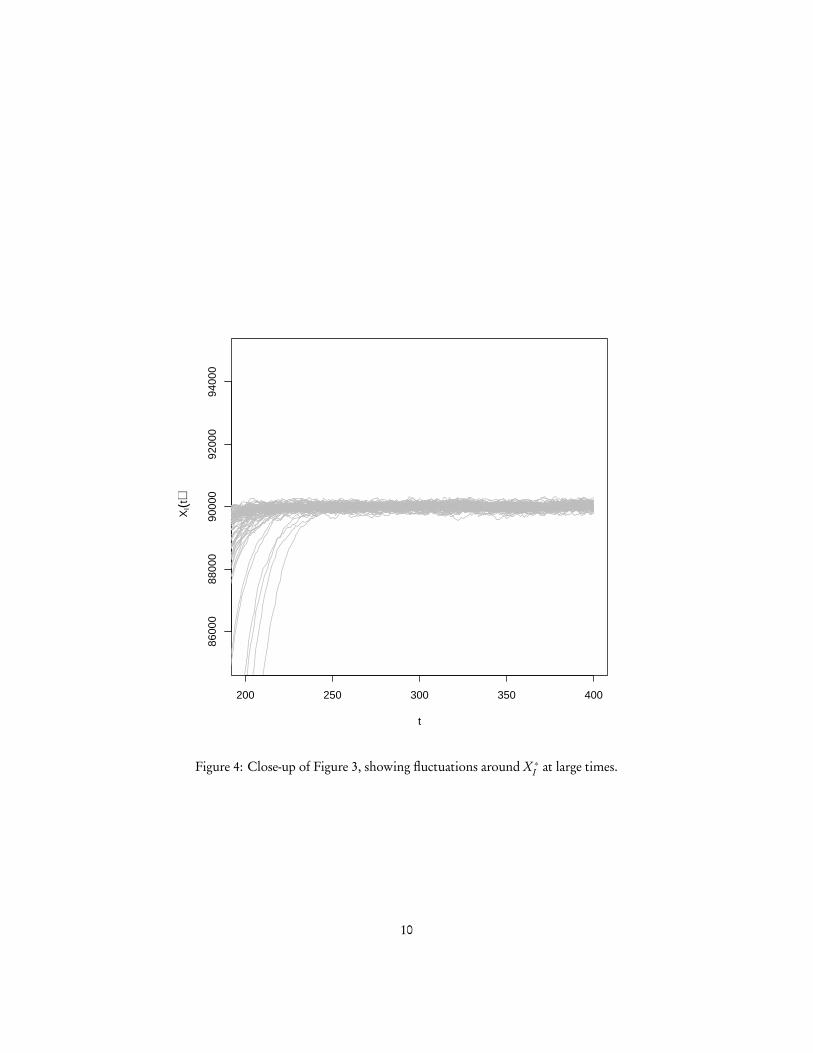
Figure 4: Close-up of Figure 3, showing fluctuations around X ∗I at large times.

10

0 50 100 150 200

02

46

810

t

XI(t

)

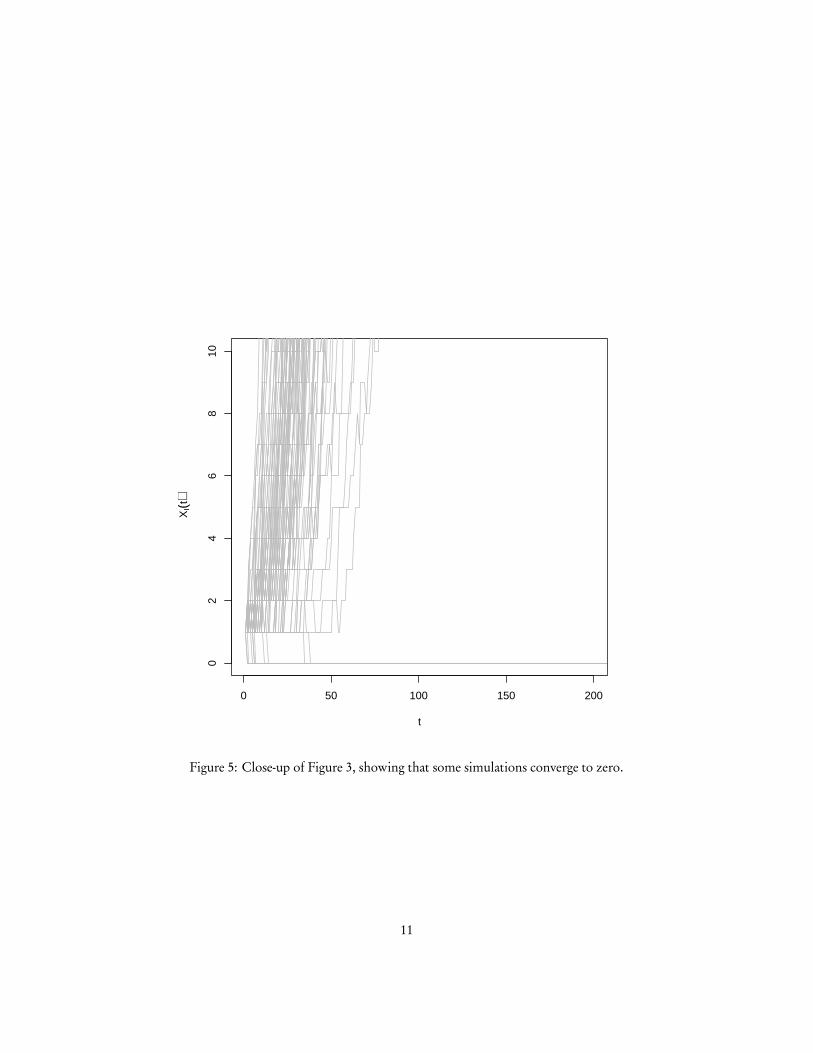
Figure 5: Close-up of Figure 3, showing that some simulations converge to zero.

11

And no matter how big XI gets, there is always some probability that it will eventu-ally reach 1, and then in turn 0. So XI = 0 is the only closed, irreducible set of states.Consequently, the disease will always die out eventually in an SIS model. It will, how-ever, generally take a very long time to do so, and in the meanwhile it will spend mostof its time oscillating around X ∗I .

2.3 SIR, SEIR, etc.It is easy, and often convenient, to add more compartments to epidemic models of thissort. In an SIR model, for example, the third compartment, R, stands for “removed”or “recovered”, depending on whether we think of individuals in that compartmentas having died off, or as having acquired immunity. The basic dynamics are

pSI = αXI (20)pI R = ρ (21)PSR = 0 (22)pI S = 0 (23)PRI = 0 (24)pRS = 0 (25)

I will let you check that the only absorbing state is XR = n, and also let you workout both the deterministic approximation and simulate some trajectories on the waythere.

A related wrinkle is to add an intermediate compartment between S and I , say Efor “exposed”, in which someone is not yet showing symptoms. Individuals in com-partment E might or might not be infectious themselves (and, if so, might be moreor less infectious than those in compartment I ). If one wants to have characteristiclengths of time for each phase of the disease, one can add even more compartments,say I1, I2, . . . Iτ , with automatic progression from one to the next.

3 SpaceThe easiest way to handle space in a compartment model is to say that you have r1types or classes of individuals across r2 locations, so that the r = r1 r2 compartmentstrack combinations of types and locations. Migration from one location to another isthen just another kind of transition. The transition rates can be made to be functionsof the counts of types only in the same location (e.g., S’s in location 1 can only beinfected by I ’s in location 1), or global aggregates calculated across all location, orsome combination of both of these.

This approach will work poorly when the number of locations r2 will becomecomparable to the population size n, since then most locations will have a count of 0for most types, and you would be better off using a different, more individual-basedmodel.

12

4 AsymptoticsWe haven’t discussed what happens as n→∞. Basically, a compartment model con-verges on a system of ordinary differential equations.

Said a bit less baldly, suppose that the transition rates pi j (X ) are all of the formpi j (X ) = ρi j (X /n)h, where h represents the amount of time that passes from onevalue of X to the next. Notice that we are assume that the transition rates are re-ally functions of the distribution of individuals across the compartments, and not thenumbers in compartments — that we get the same rate of infection when n = 20 andXI = 10 as when n = 2000 and XI = 1000. Finally, we fix a finite, but perhaps large,interval of time T . Then what we find is that the trajectory of the compartmentmodel between time 0 and time T approaches the solution of a differential equation.If we say that x(t ) is the solution to

d xi

d t=∑

j

ρ j i (x(t ))x j (t )−ρi j (x(t ))xi (t ) (26)

then, as n→∞ and h→ 0, the random sequence X (h)/n,X (2h)/n,X (3h)/n, . . .X (T )/ncomes closer and closer to the deterministic function x on the interval [0,T ] (withhigh probability).

This is the trick that I used above, when I invoked “deterministic approximations”to the epidemic models. For instance, in the SI model, the limiting trajectory for(XS (t )/n,XI (t )/n) is given by

d xS

d t= −axS (t )(1− xS (t )) (27)

d xI

d t= axI (t )(1− xI (t )) (28)

xS (t )+ xI (t ) = 1 (29)(30)

and solving this differential equation does indeed give us sigmoidal growth curves.(Can you work out how the a here relates to the α in the stochastic, finite-n versionof the SI model?)

It is important that the convergence only holds over finite times [0,T ]. Basically,this is because infinite time gives a stochastic process infinitely many opportunitiesto do arbitrarily improbable things, so they will eventually. In particular, in the SISmodel, the limiting behavior is

d xI

d t= axI (t )(1− xI (t ))− g xI (t ) (31)

and not extinction.

13

5 Demography: Birth, Aging, and DeathSo far, we have considered models where the population size n is constant. Most realpopulations change in size, and an important application of compartment models isto demography, where what we really care about is how n changes over time. Thethree processes which change n are birth, death, and migration.

The SIR model shows how to handle death: we can treat “being dead” as justanother compartment, say R6. Individuals in compartment i transition to this com-partment at some rate δi , and there are no transitions out of this compartment. De-mographers typically define the mortality rate as the number of deaths per 1000individuals per year, which you can translate into a probability per person per unittime (depending on the time-scale of your model). Yi R(t ) would be the random vari-able which counted the actual number of deaths among members of compartment iin time-period t . If this sort of formal simplicity isn’t needed, however, we can simplyintroduce a new variable Di (t ) for deaths in compartment i in period t .

Migration can be handled similarly, by introducing a new compartment for “leav-ing for the rest of the world”. If both in- and out- migration are possible, then weneed to model the flow of immigrants.

Birth, however, requires a slightly special treatment in these models. The diffi-culty is that parents are (typically) still around. The easiest way to handle this is tointroduce a new set of variables, Bi j (t ), which count the number of new births intocompartment j from parents in compartment i7 If individuals can only be born oneat a time, then we can make Bi j binomial reflecting a certain rate of parentage for in-dividuals in compartment i . If there are a non-trivial number of twins, triplets, etc.,it might be better to use something like a Poisson distribution.

The model thus looks like this:

Yi j (t + 1) ∼ Binom(Xi (t ), pi j (X (t ))) (32)

Di (t + 1) ∼ Binom(Xi (t ),δi (X (t ))) (33)Bi j (t + 1) ∼ Binom(Xi (t ),βi j (X (t ))) (34)

Xi (t + 1) = Xi (t )−Di (t + 1)+Bi i (t + 1)+∑

j 6=i

B j i (t + 1)+Y j i (t + 1)−Yi j (t + 1)(35)

In human demography, and to a lesser extent in population ecology, we need afairly large number of compartments, which track combinations of age and sex. De-mographers conventionally work with 5-year age brackets, so that there is a compart-ment for females age 0–5 and for males age 0–5, for females age 6–10 and for males age6–10, and so on all down the line. The transition probabilities are very simple: everyindividual who does not die moves into the next age group (and the same sex), withprobability 1. It is the age-specific death rates δi which let us model realistic distribu-tions of life-span; without them, we’d have geometric distributions of longevity.

6Saying that R stands for “removed” is euphemistic.7I am writing as though individuals have only one parent, which of course isn’t true for (most) verte-

brates, including human beings, but the reasons for this will become apparent shortly.

14

Births can only happen into the 0–5 age brackets, so Bi j = 0 unless j is one ofthose two brackets. Because only females give birth, Bi j = 0 unless i is a female agebracket of child-bearing age. In many applications, the age-fertility rates βi j will betaken to be constant, but they can be allowed to vary with the number of males, oreven with the ratio of males to females, depending on the customs of the populationconcerned. Note that these rates βi j should not be confused with the total fertilityrate, which is the sum of age-specific rates across child-bearing years.

6 ChemistryChemistry provides an important application for compartment models. Here the“compartments” are different types of molecules, or chemical species, and transi-tions are the consequences of reactions. We can write the SI model in this form, withone reaction, S + I → 2I 8. We can also write the SIS model as something with tworeactions, S + I → 2I and I → S. The constant-n case corresponds to all reactionshaving the same number of molecules on both the left- and the right- hand sides (asthe SI and SIS cases do). In actual chemistry, though, it’s common for the number ofmolecules to change, as in 2H2+O2→ 2H2O (three molecules go in, two moleculescome out). The way to handle this is to use Y variables to count the number of timeseach reaction happens, and then subtract the substrates (on the left) and add the prod-ucts (on the right), so, e.g., if the hydrogen-and-oxygen-to-water reaction was the onlyone, we’d have

XH2(t + 1) = XH2

(t )− 2Y2H2+O2→2H2O (t + 1) (36)

XO2(t + 1) = XO2

(t )−Y2H2+O2→2H2O (t + 1) (37)

XH2O (t + 1) = XH2O (t )+ 2Y2H2+O2→2H2O (t + 1) (38)

(We would also typically assume that the transition rate for this reaction is ∝X 2

H2XO2

.)

7 Further readingFor a fine textbook treatment of compartment models in biology, see Ellner andGuckenheimer (2006), which includes a good chapter on epidemic models, and refer-ences to the further literature.

8 ExercisesTo think through, as complements to the reading, not to hand in.

8A reaction like this, where the species I is involved in a process which makes more of the same species,is called autocatalytic.

15

1. Compartment-model state spaces are very large Fix n. A possible state X is a vec-tor of non-negative integers [X1,X2, . . .Xr ], with the constraint that

∑ri=1 Xi =

n. Prove that the number of such vectors is�

n+ r − 1n

�

.

(a) Imagine writing out a line of n dots, and inserting r − 1 vertical bars be-tween the dots, with the possibility of bars being next to each other. Callthe number of dots to the left of the left-most bar X1, the number of dotsbetween that first bar and the second X2, and so on. Convince yourselfthat every arrangement of dots and bars corresponds to a valid value of X ,and that every valid value of X can be represented in this way.

(b) Show that the number of arrangements of dots and bars is equal to choos-ing n locations for dots out of n+ r − 1 places.

(c) Show that�

n+ r − 1n

�

=�

n+ r − 1r − 1

�

.

(d) Use Stirling’s approximation, log n! ≈ n log n, to show that as n growswith r fixed, the size of the state space grows like n r−1.

2. Randomly-varying transition rates across individuals and over-dispersion Supposethat each individual in compartment i has its own, random transition rate Pi j

for moving to compartment j , with E�

Pi j

�

= pi j and Var�

Pi j

�

= vi j . Show

that Var�

Yi j (t + 1)|X (t )�

=Xi (pi j (1− pi j )+ vi j ).

3. Show the following for the SI model of §2.1.

(a) XI = 0 and XI = n are absorbing states.

(b) There are no other absorbing states.

(c) An absorbing state forms a closed, irreducible set of states. (This is a gen-eral fact about Markov chains.)

(d) This chain has no other closed, irreducible sets.

(e) With probability 1, either XI (t )→ 0 or XI (t )→ n.

4. For the SIS model, calculate E�

XI (t + 1)−XI (t )|XI (t ) =X ∗I + ε�

in terms ofn, α, ρ and ε, and show that (for small ε) it has the opposite sign from ε.

5. (a) Prove that if the probability of an event happening on each time step is aconstant p, and successive time-steps are independent, the number of stepswe need to wait for the event to happen has a geometric distribution. Findthe parameter in terms of p.

ReferencesDawkins, Richard (1976). The Selfish Gene. Oxford: Oxford University Press.

16

Ellner, Stephen P. and John Guckenheimer (2006). Dynamic Models in Biology. Prince-ton, New Jersey: Princeton University Press.

Li, Ming and Paul M. B. Vitányi (1997). An Introduction to Kolmogorov Complexityand Its Applications. New York: Springer-Verlag, 2nd edn.

Lotka, Alfred J. (1924). Elements of Physical Biology. Baltimore, Maryland: Williamsand Wilkins. Reprinted as Elements of Mathematical Biology, New York: DoverBooks, 1956.

Rogers, Everett M. (2003). Diffusion of Innovations. New York: Free Press, 5th edn.

Ruelle, David (1991). Chance and Chaos. Princeton, New Jersey: Princeton Univer-sity Press.

Salmon, Wesley C. (1984). Scientific Explanation and the Causal Structure of the World.Princeton: Princeton University Press.

Siegfried, André (1960/1965). Germs and Ideas: Routes of Epidemics and Ideologies. Ed-inburgh: Oliver and Boyd. Translated by Jean Heanderson and Mercedes Clarasófrom Itinéraires de Contagions: Epidémies et idéologies (Paris: Librarie ArmandColin).

17