1 OF 13

Statistics 22_multiple_regression.pdf

Michael Hallstone, Ph.D. hallston@hawaii.edu

Lecture 22: Multiple Regression (Ordinary Least Squares -- OLS)

Some Common Sense Assumptions for Multiple Regression (these are truncated for simplicity):

• Dependent variable is interval or ratio (not nominal or ordinal). • Ratio level variables are best for the other independent variables • Nominal and ordinal independent variables can be used if made into “dummy” variables:

o Nominal or ordinal variables can be used as independent variables if the characteristic of interest is coded 1 and the other values are coded zero. For example in criminology it is known that, as a group, men commit more violent crime than women. So if we were interested in the affect of “maleness” on criminality we would code men =1 and women=0. If we thought having a college degree (or higher) might increase income, we would code college =1 and all lower educational categories =0. Thus we pretend it is a ratio variable where 1=100% of our characteristic of interest and 0=0% of the characteristic.

• The data comes from a random sample. • There is a logical relationship between the variables.

Introduction

You must understand lecture 21 on Simple Regression for this lecture to make any sense. The same basic idea applies. In simple regression we saw if we could “predict” the outcome of a dependent variable (usually called y) using another independent variable (usually called x). In multiple regression we can use many independent variables

Simple regression only allowed us to use one independent variable to explain our dependent variable. In the previous lecture I made the argument that anything worth explaining in the social world has multiple causes not just one. To quote the previous lecture,

As you might guess, the social world is very complex most social phenomenon are not caused or explained by single factors. I can’t think of a single social science question “Why do people do x?” that can be explained by a single factor. Why people use drugs, commit murder, abuse children, spend money, visit Hawaii are all poorly explained by single factors or variables.

Thus the term multiple regression comes from the notion that we are looking at how multiple independent variables influence the dependent variable.

2 OF 13

For example using SAT scores alone to “predict” college GPA is inadequate. There are a whole lot of other things besides SAT scores that predict GPA. What about high School GPA as a measure of college preparedness? How about including number of hours studied a week? How about how many hours a week a person works? Obviously all sorts of independent variables work together to “cause” GPA to rise or fall – not a single factor or variable. This aint a math course

The math on multiple regression is daunting. Even way back in the dark ages of the mid 1990s computers routinely took several minutes to spit out multiple regression output. Obviously computer-processing power is much faster and this is no longer an issue but suffice it to say that if it took a computer several minutes, doing it by hand is a nightmare! Thus I skip the math and use SPSS.

Example of Multiple Linear “Ordinary Least Squares” Regression

We will use the same example of the number of surfers in the water at Waimea Bay, home of the legendary Eddie Aikau big wave surf contest. We will look at several factors that might predict how many surfers are in the water at Waimea Bay: wave height, wind direction, swell direction, and whether or not the pro surfing tour is on the island.

Real Waimea – no thanks! …For a sense of size that’s a 9-10 foot surfboard.

3 OF 13

Dependent variable: number of surfers in the water at Waimea

The dependent variable (or y) is “the number of surfers in the water at Waimea Bay.” Independent variables: wave size, wind, swell, and pros looking to be famous

A little more background to understand the logic of these independent variables is in order.

Wave height

Waves are like icebergs. It is not only what you see above the water; they have depth below the water too. A wave breaks when its bottom feels the ocean floor and slows down. This causes the top of the wave to pitch forward or break. Surfers catch the waves just when they start to break. So Waimea is a deep-water surf spot. All big wave surf spots are. So the waves at Waimea do not even start to break until the waves are large and the bottom of the wave feels the deep ocean floor in Waimea Bay.

The perspective from the Waimea Point – legendary surfer Brock Little hoping make it to the center of the Waimea Bay

Wind and swell direction matter in surfing

Truly giant waves like those at Waimea are really dangerous in the best of conditions. In case those pictures did not make an impression, “No really!” The waves at Waimea are extremely dangerous. In my younger days I found waves with 15-foot faces to look like small mountains moving through the water. The faces of these immense waves are forty feet, even higher. They are as big as

4 OF 13

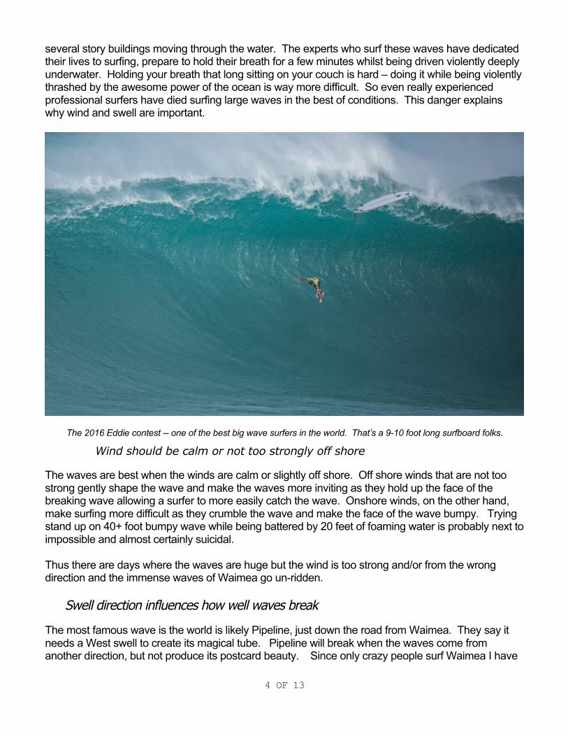
several story buildings moving through the water. The experts who surf these waves have dedicated their lives to surfing, prepare to hold their breath for a few minutes whilst being driven violently deeply underwater. Holding your breath that long sitting on your couch is hard – doing it while being violently thrashed by the awesome power of the ocean is way more difficult. So even really experienced professional surfers have died surfing large waves in the best of conditions. This danger explains why wind and swell are important.

The 2016 Eddie contest -- one of the best big wave surfers in the world. That’s a 9-10 foot long surfboard folks.

Wind should be calm or not too strongly off shore

The waves are best when the winds are calm or slightly off shore. Off shore winds that are not too strong gently shape the wave and make the waves more inviting as they hold up the face of the breaking wave allowing a surfer to more easily catch the wave. Onshore winds, on the other hand, make surfing more difficult as they crumble the wave and make the face of the wave bumpy. Trying stand up on 40+ foot bumpy wave while being battered by 20 feet of foaming water is probably next to impossible and almost certainly suicidal. Thus there are days where the waves are huge but the wind is too strong and/or from the wrong direction and the immense waves of Waimea go un-ridden. Swell direction influences how well waves break

The most famous wave is the world is likely Pipeline, just down the road from Waimea. They say it needs a West swell to create its magical tube. Pipeline will break when the waves come from another direction, but not produce its postcard beauty. Since only crazy people surf Waimea I have

5 OF 13

no idea what swell direction it “likes,” but let us pretend Waimea is more fun to surf when the waves come from a favorable swell direction.

Pipeline on a clean West swell

The North Shore is even more crowded when the pro surf tour is in town

The North Shore of Oahu is the proving ground of professional surfing. It is not hyperbole to say that a professional surfer in not considered world class until they show they can surf the large dangerous waves of the North Shore. Surfers make their money by sponsorships and sponsors demand to see pictures and videos of their surfers surfing on the North Shore. When Waimea is breaking, it is almost mandatory for a professional surfer to be photographed surfing its legendary waves. So when the professional surfing tour is on Oahu during November and December we would expect more suffers in the water at Waimea.

The crowds on a “super small” day. Imagine that! This is not considered “real Waimea.”

6 OF 13

A review of the variables

Dependent variable (y)

• number of surfers in the water at Waimea

Independent variables (x)

• x1 = wave height (in feet)

• x2 = bad wind or good wind? (bad wind=1 good wind=0)

• x3 = pro tour in town? (pro tour in town=1 pro tour out of town=0)

• x4 = swell direction (optimum swell direction =1 other swell direction=0)

The regression equation would look like this

y-hat= a + b1x1 + b2x2 + b3x3 + b4x4 (where a = y intercept and y-hat = estimated number of surfers in the water at Waimea)

(The b’s in the equation are slopes of each independent variable and will be explained below)

7 OF 13

SPSS output

Is the model significant? Look at the ANOVA box under “Sig.”

That is the p-value of the entire model. The model refers to whether or not all of the independent variables combined account for a significant amount of variation in the dependent variable.

Decision rule for statistical significance using p-value

• If p-value < α or “alpha” it is significant! [Typically we use alpha =.05] • If p-value >= α or “alpha” it is NOT significant! [Typically we use alpha =.05]

So....

• If p-value < .05 ”it is significant! If p-value >= .05 it is NOT significant!

Our p value is small. It is not really .000 but p<. 001, which is less than .05 so our model is significant.

8 OF 13

Finding the slope of the independent variables – unstandardized coefficients

Each independent variable has a number that represents a slope. In SPSS they are called unstandardized coefficients and found under B in the Coefficients box. The slopes or unstandardized coefficients are meaningful only if the overall model is statistically significant.

Coefficientsa

Model

Unstandardized Coefficients

Standardized Coefficients

t Sig. B Std. Error Beta 1 (Constant) .764 13.631 .056 .956

Wave height at Waimea 1.410 .541 .334 2.608 .013

bad wind =1 -20.903 7.235 -.408 -2.889 .007 pro tour in town=1 14.857 5.139 .272 2.891 .007

best swell direction=1

7.544 6.338 .115 1.190 .242

a. Dependent Variable: number of surfers in water

Recall y-hat= a + b1x1 + b2x2 + b3x3 + b4x4 (where a = y intercept)

Dependent variable (y)

• number of surfers in the water at Waimea

Independent variables (x)

• x1 = wave height (in feet) • x2 = bad wind or good wind? (bad wind=1 good wind=0) • x3 = pro tour in town? (pro tour in town=1 pro tour out of town=0) • x4 = swell direction (optimum swell direction =1 other swell direction=0)

Thus our regression equation is

y-hat= .764 + 1.410x1 + -20.903x2 + 14.857x3 + 7.544x4

Now we need to see which of the independent variables have a statistically significant effect. We use the p-value under Sig in the far right column of the Coefficients box above.

9 OF 13

• x1 = wave height p-value =.013 or 1.3% so it’s less than .05 or 5% and statistically significant • x2 = bad wind or good wind p-value =.007 or 0.7% so it’s less than .05 or 5% and

statistically significant • x3 = pro tour in town p-value =.007 or 0.7% so it’s less than .05 or 5% and statistically

significant • x4 = swell direction p-value =.242 or 24.2% so it’s greater than .05 or 5% and not statistically

significant – this variable has no effect

Interpreting the slopes of the independent variables – unstandardized coefficients

Recall, the overall model must be statistically significant for our interpretation below to make sense. If the overall model is not significant the interpretation of the slopes is meaningless. Recall above our model has p<.001 so it is statistically significant.

y-hat= .764 + 1.410x1 + -20.903x2 + 14.857x3 + 7.544x4

To quote my colleague Dr. Michael Delucchi, “In multiple regression each slope represents the impact of the independent variable when all other independent variables are held constant. It tells us the impact each independent variable has over and above the effects of remaining independent variables.”

Interpreting the effect of ratio level independent variables on the dependent variable

• x1 = wave height b1 =1.41 When all other independent variables are held constant, every one-foot increase in wave height the number of surfers in the water increases by 1.41. (There is no such thing as 1.41 surfers so if you wanted to round this to “approximately 1 surfer” that would make sense.) An increase in waves increases the number of surfers in the water.

Interpreting the effect “dummy” independent variables on the dependent variable

Recall that the variables below were nominal variables coded 1 and 0, where 1= the characteristic of interest. We pretend they are ratio where 1=100% of the characteristic of interest and 0=0% of the characteristic of interest.

• x2 = bad wind or good wind? (bad wind=1 good wind=0) • x3 = pro tour in town? (pro tour in town=1 pro tour out of town=0) • x4 = swell direction (optimum swell direction =1 other swell direction=0)

Dummy variables are interpreted differently. When the dummy variable =1 the slope is the effect it has on the dependent variable.

• x2 = bad wind or good wind b2 = -20.903 the minus sign is meaningful! When all other independent variables are held constant, when there is a bad wind (as compared to a good wind), the number of surfers in the water decreases by 20.903 surfers.

10 OF 13

(There is no such thing as 20.903 surfers so if you wanted to round this to “approximately 21 surfers” that would make sense.) The minus sign means the affect on the dependent variable is negative. The number of surfers goes down when the wind is bad.

• x3 = pro tour in town b2 = 14.857 When all other independent variables are held constant, when the pro tour is in town (as

compared to when the pro tour is not in town), the number of surfers in the water increases by 14.857 surfers. (There is no such things as 14.857 surfers, so if you wanted to round that to “approximately 15 surfers” that would make sense.) Having the pro tour in town increases the crowd in the water.

• x4 = swell direction since p-value =.242 or 24.2% so it’s greater than .05 or 5% and not

statistically significant – this variable has no effect. So whether or not the waves are coming from the optimum swell direction for Waimea has no effect on the number of surfers in the water!

11 OF 13

Standardized slope or standardized coefficients –SPSS calls them “Beta”

Recall, the overall model must be statistically significant for our interpretation below to make sense.

Recall we are looking at the effect of several independent variables on the dependent variable – sometimes called a “model.” We need a way to figure out which independent variable in the model has the strongest effect on the dependent variable. Of the variables which are statistically significant (p<.05), the largest standardized coefficient (in absolute value) has the largest relative effect on the dependent variable.

In our example we would wonder what has a greater effect on the number of surfers at Waimea – wave height, wind, having pros in town? (We know from above that swell direction has no effect whatsoever.)

To do this we standardize the slopes or coefficients. The formula is

Beta = b(sx/sy) where

b=slope of the independent variable sx= standard deviation of the independent variable sy= standard deviation of the dependent variable

Thus the standardized slope for the size of the waves is

Beta wave height = b(s wave height /s number of surfers in the water)

Beta wave height = 1.41(6.04872 / 25.53345)

Beta wave height = 1.41(.0.2369) Beta wave height =.334

12 OF 13

Standardized Slopes or Coeffients or Beta in SPSS

Coefficientsa

Model

Unstandardized Coefficients

Standardized Coefficients

t Sig. B Std. Error Beta 1 (Constant) .764 13.631 .056 .956

Wave height at Waimea

1.410 .541 .334 2.608 .013

bad wind =1 -20.903 7.235 -.408 -2.889 .007 pro tour in town=1 14.857 5.139 .272 2.891 .007

best swell direction=1 7.544 6.338 .115 1.190 .242

a. Dependent Variable: number of surfers in water

Which independent variable in the model has the strongest effect on the dependent variable?

Strength of standardized slopes in descending order:

• Beta x2 = bad wind or good wind = -0.408 • Beta x1 = wave height = 0.334 • Beta x3 = pro tour in town = 0.272

So in absolute value -0.408 is the “largest” number and having a bad wind has the greatest effect of all the independent variables on the number of surfers in the water. Perhaps this makes sense as when the wind is bad, surfing Waimea is literally death defying and perhaps suicidal. So “real” Waimea only breaks when the waves are huge and dangerous. If the waves are enormous and the wind is strongly onshore, there are zero surfers in the water because it’s too dangerous.

13 OF 13

Interpreting standardized slopes or coefficients or Beta

The plain English on this one is a little whacky as it involves the language of standard deviations. (Recall a standard deviation produces a number that answers the question “On average how much do the data points differ from the mean.” So the standard deviation is the average deviation from the mean.)

• Beta x2 = bad wind or good wind = - 0.408 the minus sign matters! With the other independent variables held constant, when there is a bad wind (as compared to when there is a good wind), there is a -0.408 standard deviation decrease in the number of surfers in the water.

• Beta x1 = wave height = 0.334

With the other independent variables held constant, for every increase of one standard deviation in wave height, there is a 0.334 standard deviation increase in the number of surfers in the water.

• Beta x3 = pro tour in town = 0.272 With the other independent variables held constant, when the pro tour is in town (as compared to when the pro tour is not in town), there is a 0.272 standard deviation increase in the number of surfers in the water.