lecture 22 : nonhomogeneous linear equations (section 17.2)apilking/math10560/lectures/lecture...
TRANSCRIPT

NonHomogeneous Second Order Linear Equations (Section 17.2) Example Polynomial Example Exponentiall Example Trigonometric Troubleshooting G(x) = G1(x) + G2(x).
NonHomogeneous Linear Equations (Section 17.2)
The solution of a second order nonhomogeneous linear differential equation ofthe form
ay ′′ + by ′ + cy = G(x)
where a, b, c are constants, a 6= 0 and G(x) is a continuous function of x on agiven interval is of the form
y(x) = yp(x) + yc(x)
where yp(x) is a particular solution of ay ′′ + by ′ + cy = G(x) and yc(x) is thegeneral solution of the complementary equation/ correspondinghomogeneous equation ay ′′ + by ′ + cy = 0.
I Since we already know how to find yc , the general solution to thecorresponding homogeneous equation, we need a method tofind a particular solution, yp, to the equation. One such methods is
described below. This method may not always work. A second methodwhich is always applicable is demonstrated in the extra examples in yournotes.
Annette Pilkington Lecture 22 : NonHomogeneous Linear Equations (Section 17.2)

NonHomogeneous Second Order Linear Equations (Section 17.2) Example Polynomial Example Exponentiall Example Trigonometric Troubleshooting G(x) = G1(x) + G2(x).
The method of Undetermined Coefficients
We wish to search for a particular solution to ay ′′ + by ′ + cy = G(x).If G(x) is a polynomial it is reasonable to guess that there is a particularsolution, yp(x) which is a polynomial in x of the same degree as G(x) (becauseif y is such a polynomial, then ay ′′ + by ′ + c is also a polynomial of the samedegree.)Method to find a particular solution: Substitute yp(x) = a polynomial ofthe same degree as G into the differential equation and determine thecoefficients.
Example Solve the differential equation: y ′′ + 3y ′ + 2y = x2.
I We first find thesolution of the complementary/ corresponding homogeneous equation,
y ′′ + 3y ′ + 2y = 0:Auxiliary equation: r 2 + 3r + 2 = 0Roots: (r + 1)(r + 2) = 0 → r1 = −1, r2 = −2. Distinct real roots.Solution to corresponding homogeneous equation:
yc = c1er1x + c2e
r2x = c1e−x + c2e
−2x .
Annette Pilkington Lecture 22 : NonHomogeneous Linear Equations (Section 17.2)

NonHomogeneous Second Order Linear Equations (Section 17.2) Example Polynomial Example Exponentiall Example Trigonometric Troubleshooting G(x) = G1(x) + G2(x).
Undetermined coefficients Example (polynomial)
y(x) = yp(x) + yc(x)
Example Solve the differential equation: y ′′ + 3y ′ + 2y = x2.
yc(x) = c1er1x + c2e
r2x = c1e−x + c2e
−2x
We now need a particular solution yp(x).
I We consider a trial solution of the form yp(x) = Ax2 + Bx + C .
I Then y ′p(x) = 2Ax + B, y ′′p (x) = 2A.
I We plug y ′′p , y ′p and yp into the equation to get2A + 3(2Ax + B) + 2(Ax2 + Bx + C) = x2
→ 2Ax2 + (6A + 2B)x + (2A + 3B + 2C) = x2.
I Equating coefficients, we get
2A = 1→ A =1
2, 6A + 2B = 0, 2A + 3B + 2C = 0.
I Plugging the value for A into the middle equation, we get
3 + 2B = 0 → B = −3
2.
Annette Pilkington Lecture 22 : NonHomogeneous Linear Equations (Section 17.2)

NonHomogeneous Second Order Linear Equations (Section 17.2) Example Polynomial Example Exponentiall Example Trigonometric Troubleshooting G(x) = G1(x) + G2(x).
Undetermined coefficients Example (polynomial)
y(x) = yp(x) + yc(x)
Example Solve the differential equation: y ′′ + 3y ′ + 2y = x2.
yc(x) = c1er1x + c2e
r2x = c1e−x + c2e
−2x
We now need a particular solution yp(x).
I Let us assume yp(x) = Ax2 + Bx + C .
I Then y′p (x) = 2Ax + B, y′′p (x) = 2A.
I We plug y′′p , y′p and yp into the equation to get 2A + 3(2Ax + B) + 2(Ax2 + Bx + C) = x2
→ 2Ax2 + (6A + 2B)x + (2A + 3B + 2C) = x2.
I Equating coefficients, we get 2A = 1→ A =1
2, 6A + 2B = 0, 2A + 3B + 2C = 0.
I Plugging the value for A into the middle equation, we get 3 + 2B = 0→ B = −3
2.
I Using values for A and B in the third equation, we get
1− 92
+ 2C = 0 → C =7
4.
Annette Pilkington Lecture 22 : NonHomogeneous Linear Equations (Section 17.2)

NonHomogeneous Second Order Linear Equations (Section 17.2) Example Polynomial Example Exponentiall Example Trigonometric Troubleshooting G(x) = G1(x) + G2(x).
Undetermined coefficients Example (polynomial)
y(x) = yp(x) + yc(x)
Example Solve the differential equation: y ′′ + 3y ′ + 2y = x2.
yc(x) = c1er1x + c2e
r2x = c1e−x + c2e
−2x
We now need a particular solution yp(x).
I Trial Solution: yp(x) = Ax2 + Bx + C .
I Then y′p (x) = 2Ax + B, y′′p (x) = 2A.
I We plug y′′p , y′p and yp into the equation to get 2A + 3(2Ax + B) + 2(Ax2 + Bx + C) = x2
→ 2Ax2 + (6A + 2B)x + (2A + 3B + 2C) = x2.
I A =1
2, B = −3
2, C =
7
4
I Hence a particular solution is given by yp =1
2
hx2 − 3x +
7
2
i,
I and the general solution is given by
y = yp + yc =1
2
hx2 − 3x +
7
2
i+ c1e
−x + c2e−2x .
Annette Pilkington Lecture 22 : NonHomogeneous Linear Equations (Section 17.2)

NonHomogeneous Second Order Linear Equations (Section 17.2) Example Polynomial Example Exponentiall Example Trigonometric Troubleshooting G(x) = G1(x) + G2(x).
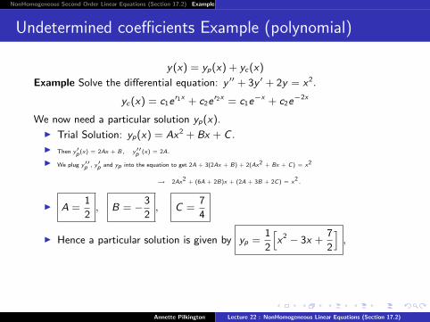
G (x) = Cekx . Example (Exponential)
We wish to search for a particular solution to ay ′′ + by ′ + cy = G(x).If G(x) is of the form Cekx , where C and k are constants, then we use a trial
solution of the form yp(x) = Aekx and solve for A if possible.
Example Solve y ′′ + 9y = e−4x .
I We first find the solution of the corresponding homogeneous equation,y ′′ + 9y ′ = 0:Auxiliary equation: r 2 + 9 = 0Roots: r 2 = −9 → r1 = 3i , r2 = −3i . Complex roots.Solution to corresponding homogeneous equation :
yc = c1 cos(3x) + c2 sin(3x) .
I Next we find a particular solution. Our trial solution is of the form
yp(x) = Ae−4x .
I y ′p(x) = −4Ae−4x , y ′′p (x) = 16Ae−4x .
I We plug y ′′p , y ′p and yp into the equation to get
16Ae−4x + 9Ae−4x = e−4x → e−4x [16A + 9A] = e−4x .
I Since e−4x > 0, we can cancel to get 25A = 1 A =1
25.
Annette Pilkington Lecture 22 : NonHomogeneous Linear Equations (Section 17.2)

NonHomogeneous Second Order Linear Equations (Section 17.2) Example Polynomial Example Exponentiall Example Trigonometric Troubleshooting G(x) = G1(x) + G2(x).
G (x) = Cekx . Example (Exponential)
We wish to search for a particular solution to ay ′′ + by ′ + cy = G(x).If G(x) is of the form Cekx , where C and k are constants, then we use a trial
solution of the form yp(x) = Aekx and solve for A if possible.
Example Solve y ′′ + 9y = e−4x .
I yc = c1 cos(3x) + c2 sin(3x) .
I Next we find a particular solution. Our trial solution is of the form
yp(x) = Ae−4x .
I y′p (x) = −4Ae−4x , y′′p (x) = 16Ae−4x .
I We plug y′′p , y′p and yp into the equation to get
16Ae−4x + 9Ae−4x = e−4x → e−4x [16A + 9A] = e−4x.
I Since e−4x > 0, we can cancel to get 25A = 1 A =1
25.
I Hence a particular solution is given by : yp =1
25e−4x ,
I General solution: y = yp + yc =1
25e−4x + c1 cos(3x) + c2 sin(3x)
Annette Pilkington Lecture 22 : NonHomogeneous Linear Equations (Section 17.2)

NonHomogeneous Second Order Linear Equations (Section 17.2) Example Polynomial Example Exponentiall Example Trigonometric Troubleshooting G(x) = G1(x) + G2(x).
G (x) = C cos kx or C sin kx . Example (Trigonometric)
If G(x) is of the form C cos kx or C sin kx , where C and k are constants, thenwe use a trial solution of the form yp(x) = A cos(kx) + B sin(kx) and solve forA and B if possible.Below we use the fact that if K1 cos(αx) + K2 sin(αx) = 0 for constantsK1,K2, α, where α 6= 0, Then we must have K1 = K2 = 0.
Example Solve y ′′ − 4y ′ − 5y = cos(2x).
I We first find the solution of the corresponding homogeneous equation,y ′′ − 4y ′ − 5y = 0:Auxiliary equation: r 2 − 4r − 5 = 0Roots: (r + 1)(r − 5) = 0 → r1 = −1, r2 = 5. Distinct real roots.
Solution to corresponding homogeneous equation : yc = c1e−x + c2e
5x .
I Next we find a particular solution. Our trial solution takes the form:yp(x) = A cos(2x) + B sin(2x).
I We plug y ′′p , y ′p and yp into the equation to get−4A cos(2x)− 4B sin(2x)− 4[−2A sin(2x) + 2B cos(2x)]− 5[A cos(2x) +B sin(2x)] = cos(2x)
I Tidying up, we get(−4A− 8B − 5A− 1) cos(2x) + (−4B + 8A− 5B) sin(2x) = 0 →(−9A− 8B − 1) cos(2x) + (−9B + 8A) sin(2x) = 0.
Annette Pilkington Lecture 22 : NonHomogeneous Linear Equations (Section 17.2)

NonHomogeneous Second Order Linear Equations (Section 17.2) Example Polynomial Example Exponentiall Example Trigonometric Troubleshooting G(x) = G1(x) + G2(x).
G (x) = C cos kx or C sin kx . Example (Trigonometric)
If G(x) is of the form C cos kx or C sin kx , where C and k are constants, thenwe use a trial solution of the form yp(x) = A cos(kx) + B sin(kx) and solve forA and B if possible.Below we use the fact that if K1 cos(αx) + K2 sin(αx) = 0 for constantsK1,K2, α, where α 6= 0, Then we must have K1 = K2 = 0.
Example Solve y ′′ − 4y ′ − 5y = cos(2x).
I Solution to corresponding homogeneous equation : yc = c1e−x + c2e
5x .
I Next we find a particular solution. Our trial solution takes the form: yp(x) = A cos(2x) + B sin(2x).
I We plug y′′p , y′p and yp into the equation to get
−4A cos(2x) − 4B sin(2x) − 4[−2A sin(2x) + 2B cos(2x)] − 5[A cos(2x) + B sin(2x)] = cos(2x)
I Tidying up, we get (−4A − 8B − 5A − 1) cos(2x) + (−4B + 8A − 5B) sin(2x) = 0
→ (−9A− 8B − 1) cos(2x) + (−9B + 8A) sin(2x) = 0.
I We must have −9A− 8B = 1, 8A− 9B = 0.
I From the second equation, we get B = 89A and substituting this into the
first equation, we get
−9A− 64
9A = 1 → −145
9A = 1 → A = − 9
145.
Annette Pilkington Lecture 22 : NonHomogeneous Linear Equations (Section 17.2)

NonHomogeneous Second Order Linear Equations (Section 17.2) Example Polynomial Example Exponentiall Example Trigonometric Troubleshooting G(x) = G1(x) + G2(x).
G (x) = C cos kx or C sin kx . Example (Trigonometric)
If G(x) is of the form C cos kx or C sin kx , where C and k are constants, thenwe use a trial solution of the form yp(x) = A cos(kx) + B sin(kx) and solve forA and B if possible.Below we use the fact that if K1 cos(αx) + K2 sin(αx) = 0 for constantsK1,K2, α, where α 6= 0, Then we must have K1 = K2 = 0.
Example Solve y ′′ − 4y ′ − 5y = cos(2x).
I Solution to corresponding homogeneous equation : yc = c1e−x + c2e
5x .
I Next we find a particular solution. Our trial solution takes the form: yp(x) = A cos(2x) + B sin(2x).
I From the second equation, we get B = 89A and substituting this into the first equation, we get
−9A − 649
A = 1 → − 1459
A = 1 → A = − 9
145.
I Substituting we get B = 89A → B = − 8
145.
I Hence a particular solution is given by yp = − 9145
cos(2x)− 8145
sin(2x),and the general solution is given by
y = yp + yc = − 9
145cos(2x)− 8
145sin(2x) + c1e
−x + c2e5x .
Annette Pilkington Lecture 22 : NonHomogeneous Linear Equations (Section 17.2)

NonHomogeneous Second Order Linear Equations (Section 17.2) Example Polynomial Example Exponentiall Example Trigonometric Troubleshooting G(x) = G1(x) + G2(x).
Trouble: Trial solution fits corresponding hom. eqn.
TroubleshootingIf the trial solution yp is a solution of the corresponding homogeneous equation,then it cannot be a solution to the non-homogeneous equation. In this case, wemultiply the trial solution by x (or x2 or x3 ... as necessary) to get a new trialsolution that does not satisfy the corresponding homogeneous equation. Thenproceed as above.
Example Solve y ′′ − y = ex .
I We first find the solution of the corresponding homogeneous equation,y ′′ − y = 0:Auxiliary equation: r 2 − 1 = 0Roots: (r + 1)(r − 1) = 0 → r1 = −1, r2 = 1. Distinct real roots.
Solution to corresponding homogeneous equation : yc = c1e−x + c2e
x .
I Next we find a particular solution. Note that Aex , is a solution to thecorresponding homogeneous equation and therefore cannot be a solutionto the non-homogeneous equation.
I As recommended, we use yp(x) = Axex .
I y ′p(x) = Aex + Axex , y ′′p (x) = 2Aex + Axex .
Annette Pilkington Lecture 22 : NonHomogeneous Linear Equations (Section 17.2)

NonHomogeneous Second Order Linear Equations (Section 17.2) Example Polynomial Example Exponentiall Example Trigonometric Troubleshooting G(x) = G1(x) + G2(x).
Trouble: Trial solution fits corresponding hom. eqn.
TroubleshootingIf the trial solution yp is a solution of the corresponding homogeneous equation,then it cannot be a solution to the non-homogeneous equation. In this case, wemultiply the trial solution by x (or x2 or x3 ... as necessary) to get a new trialsolution that does not satisfy the corresponding homogeneous equation. Thenproceed as above.
Example Solve y ′′ − y = ex .
I yc = c1e−x + c2e
x .
I Next we find a particular solution. Note that Aex , is a solution to the corresponding homogeneous equation and therefore
cannot be a solution to the non-homogeneous equation.
I As recommended, we use yp(x) = Axex .
I y ′p(x) = Aex + Axex , y ′′p (x) = 2Aex + Axex .
I We plug y ′′p and yp into the equation to get
2Aex + Axex − Axex = ex → 2Aex = ex → 2A = 1 → A = 1/2
I Hence a particular solution is given by yp =1
2xex
Annette Pilkington Lecture 22 : NonHomogeneous Linear Equations (Section 17.2)

NonHomogeneous Second Order Linear Equations (Section 17.2) Example Polynomial Example Exponentiall Example Trigonometric Troubleshooting G(x) = G1(x) + G2(x).
Trouble: Trial solution fits corresponding hom. eqn.
TroubleshootingIf the trial solution yp is a solution of the corresponding homogeneous equation,then it cannot be a solution to the non-homogeneous equation. In this case, wemultiply the trial solution by x (or x2 or x3 ... as necessary) to get a new trialsolution that does not satisfy the corresponding homogeneous equation. Thenproceed as above.
Example Solve y ′′ − y = ex .
I yc = c1e−x + c2e
x .
I Next we find a particular solution. Note that Aex , is a solution to the corresponding homogeneous equation and therefore
cannot be a solution to the non-homogeneous equation.
I As recommended, we use yp(x) = Axex .
I Particular solution: yp =1
2xex
I general solution: y = yp + yc =1
2xex + c1e
−x + c2ex
Annette Pilkington Lecture 22 : NonHomogeneous Linear Equations (Section 17.2)

NonHomogeneous Second Order Linear Equations (Section 17.2) Example Polynomial Example Exponentiall Example Trigonometric Troubleshooting G(x) = G1(x) + G2(x).
G (x) = G1(x) + G2(x).
To solve the equation ay ′′ + by ′ + cy = G1(x) + G2(x), we can find particularsolutions, yp1 and yp2 to of the equations
ay ′′ + by ′ + cy = G1(x), ay ′′ + by ′ + cy = G2(x)
separately. The general solution of the equationay ′′ + by ′ + cy = G1(x) + G2(x) is yp1 + yp2 + yc , where yc is the solution ofthe corresponding homogeneous equation ay ′′ + by ′ + cy = 0.
Example For the equation y ′′ + y ′ + y = x2 + ex , we use a trial solution of theform
yp = (Ax2 + Bx + C) + Dex .
Annette Pilkington Lecture 22 : NonHomogeneous Linear Equations (Section 17.2)