Lecture 23•Second order system step response

• Governing equation• Mathematical expression for step response• Estimating step response directly from

differential equation coefficients• Examples

•Related educational modules: – Section 2.5.5

Second order system step response

• Governing equation in “standard” form:

• Initial conditions:

• We will assume that the system is initially “relaxed”

Second order system step response – continued

• We will concentrate on the underdamped response:

• Looks like the natural response superimposed with a step function

tsintcose

A)t(y dd

t

n

n

22

11

Step response parameters

• We would like to get an approximate, but quantitative estimate of the step response, without explicitly determining y(t)• Several step response parameters are directly related to

the coefficients of the governing differential equation

• These relationships can also be used to estimate the differential equation from a measured step response• Model parameter estimation

Second order system step response – plot

yss

yp

0.9yss

0.1yss

tr

Steady-state response• Input-output equation:

• As t, circuit parameters become constant so:

• Circuit DC gain:

• On previous slide, note that DC gain can be determined directly from circuit.

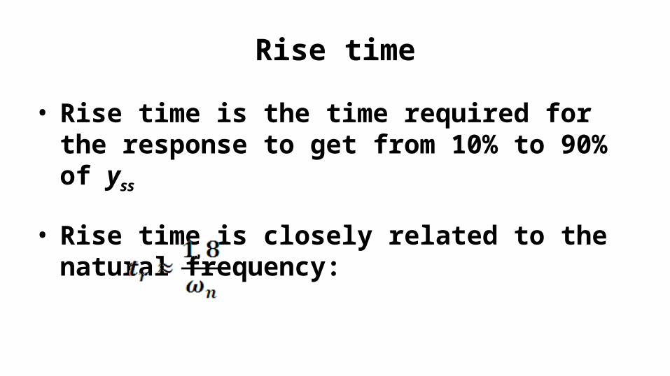
Rise time

• Rise time is the time required for the response to get from 10% to 90% of yss

• Rise time is closely related to the natural frequency:

Maximum overshoot, MP

• MP is a measure of the maximum response value

• MP is often expressed as a percentage of yss and is related directly to the damping ratio:

Maximum overshoot – continued

• For small values of damping ratio, it is often convenient to approximate the previous relationship as:

Example 1• Determine the maximum value of the current, i(t), in the

circuit below

• In previous slide, outline overall approach:– Need MP, and steady-state value– Need damping ratio to get MP– Need natural frequency to get damping ratio– Need to determine differential equation

Step 1: Determine differential equation

Step 2: Identify n, , and steady-state current

• Governing equation:

Step 3: Determine maximum current

• Damping ratio, = 0.54

• Steady-state current,

Example 2

• Determine the differential equation governing iL(t) and the initial conditions iL(0+) and vc(0+)

Example 2 – differential equation, t>0

Example 2 – initial conditions

Example 3 – model parameter estimation

The differential equation governing a system is known to be of the form:

When a 10V step input is applied to the system, the response is as shown. Estimate the differential equation governing the system.

0 0.05 0.1 0.15 0.2 0.25 0.3 0.35 0.40

0.5

1

1.5

2

2.5x 10

-3

Example 3 – find tr, MP, yss from plot

0 0.05 0.1 0.15 0.2 0.25 0.3 0.35 0.40

0.5

1

1.5

2

2.5x 10

-3

Example 3 – find differential equation

• From plot, we determined:– MP 0.25

– tr 0.05

– yss 0.002

Example 4 – Series RLC circuit

• MP 100%, n = 100,000 rad/sec (16KHz)