Prof. Eduardo A. Haddad

Lecture 3: Exploratory Spatial Data

Analysis (ESDA)

2

Key message

Spatial dependence

First Law of Geography (Waldo Tobler):

“Everything is related to everything else, but near things are more related than distant things”

3

Spatial analysis

Locational invariance Spatial analysis is not locationally invariant The results change when the locations of the

study objects change “Where” matters!

Mapping and Geovisualization Showing interesting patterns

Exploratory Spatial Data Analysis Discovering interesting patterns

Spatial Modeling Explaining interesting patterns

4

GeoDa – https://spatial.uchicago.edu/

5

ESDA

Exploratory data analysis (EDA) uses a set of techniques to:

maximize insight into a data set uncover underlying structures extract important variables detect outliers and anomalies test underlying assumptions suggest hypotheses develop parsimonious models

ESDA includes spatial attributes of the data

6

Geovisualization

Beyond mapping:

Combining map and scientific visualization methods

Exploit human pattern recognition capabilities

Statistical maps

Innovative map devices (quantile map, percentile map, box map, standard deviation map, conditional map)

Map movie

7

Exercise 1 (mapping)

Open and close a project

Load a shape file with the proper indicator (Key)

Select functions from the menu or toolbar

Make a simple choropleth map

Select items in the map

Data: Morocco (gdppc_07); Brazil_UF (Y00, G00, RG00); Brazil_MR (RENDAPC, ESGT, M1SM)

8

Exercise 2 (data)

Open and navigate the data table

Select and sort items in the table

Create new variables in the table

Data: Morocco (gdppc_03, gdppc_07)

Which regions presented the highest per capita GRP growth from 2003 to 2007 in Morocco?

Table > Calculator

9

Exercise 3 (EDA)

This exercise illustrates some basic techniques for exploratory data analysis, or EDA. It covers the visualization of the non-spatial distribution of data by means of a histogram and box plot, and highlights the notion of linking, which is fundamental in GeoDa.

Data: Brazil_UF (Y00, G00)

Histogram:

The histogram is a discrete approximation to the density function of a random variable

10

Exercise 3 (EDA)

Box plot:

It shows the median, first and third quartiles of a distribution (the 50%, 25% and 75% points in the cumulative distribution) as well as a notion of outlier.

An observation is classified as an outlier when it lies more than a given multiple of the interquartile range (the difference in value between the 75% and 25% observation) above or below respectively the value for the 75th percentile and 25th percentile. The standard multiples used are 1.5 and 3 times the interquartile range.

11

Box plot

Hinge = 1.5

Outlier

Interquartile range(25% a 75%)

Median

Mean

12

Exercise 3 (EDA)

Scatter plot:

The visualization of the bivariate association between variables can be done by means of a scatter plot

Converting the scatter plot to a correlation plot, in which the regression slope corresponds to the correlation between the two variables (as opposed to a bivariate regression slope in the default case).

Any observations beyond the value of 2 can be informally designated as outliers

13

Exercise 3 (EDA)

Conditional plots:

Conditional plots, also known as facet graphs or Trellis graphs (Becker, Cleveland, and Shyu 1996), provide a means to assess interactions between more than two variables. Multiple graphs or maps are constructed for different subsets of the observations, obtained as a result of conditioning on the value of two variables.

Conditional scatter plot

Data: Brazil_MR (RENDA=f(POP), ESGT, M1SM)

14

Exercise 4 (spatial scale and rate of density)

Inference can change with scale

Problem of spatial aggregation State versus micro-region

Intensity maps Extensive variable tends to be correlated with

size (such as area or total population) Rate or density is more suitable for a choropleth

map, and is referred to as an intensive variable.

Data: Brazil_UF (Y00) and Brazil_MR (RENDAPC, RENDA, POP)

Rates-calculated map (Raw rate; Excess risk)

15

Spatial dependence

What happens at one place depends on events in nearby places

Remember: “All things are related but nearby things are more related than distant things” (Tobler)

Categorizing Type: substantive versus nuisance Direction: positive versus negative

Issues Time versus space Inference

16

Concepts

Spatial weights

Spatial lag

Spatial autocorrelation

17

Spatial weights matrix

Definition:

N by N positive matrix W, elements wij

wij nonzero for neighbors, 0 otherwise

wii = 0, no self-neighbors

Geographic weights (contiguity, distance, general, graph-based weights)

Socio-economic weights

18

Contiguity weights

Contiguity: sharing a common boundary of non-zero length

Three views of contiguity:

rook bishop queen

rook queen

19

Exercise 5 (spatial weights)

Contiguity-based spatial weights

Create a first order contiguity spatial weights file from a polygon shape file, using both rook and queen criteria (.GAL)

Connectivity structure of the weights in a histogram

Higher order contiguity

Data: Brazil_UF; Morocco

20

Exercise 6 (spatial weights)

Distance-based spatial weights

Create a distance-based spatial weights file from a point shape file, by specifying a distance band

Adjust the critical distance

Create a spatial weights file based on a k-nearest neighbor criterion

Data: Hedonic; Brazil_UF; Morocco

21

Spatially lagged variables

Spatially lagged variables are an essential part of the computation of spatial autocorrelation tests and the specification of spatial regression models

Wy: is the average of a variable in the neighboring spatial units (e.g. WY00 is the average per capita income of the neighbors)

22

Exercise 7 (spatial lag)

Scatter plot of Y00 and WY00

Use standardized values

Data: Brazil_UF (Y00)

23

Clustering

Global characteristic

Property of overall pattern = all observations are like values more grouped in space than random

Test by means of a global spatial autocorrelation statistic

No location of the clusters determined

24

Clusters

Local characteristic

Where are the like values more grouped in space than random?

Property of local pattern = location-specific

Test by means of a local spatial autocorrelation statistic

Local clusters may be compatible with global spatial randomness

25

Spatial autocorrelation statistic

Formal test of match between value similarity and locational similarity

Statistic summarizes both aspects

Significance: how likely is it (p-value) that the computed statistic would take this (extreme) value in a spatially random pattern?

26

Attribute similarity

Summary of the similarity or dissimilarity of a

variable at different locations:

Variable y at locations i, j with i ≠ j

Measures of similarity:

Cross product: yiyj

Measures of dissimilarity:

Squared differences: (yi - yj)2

Absolute differences: │yi - yj│

27

Global spatial autocorrelation (Moran’s I)

zi = xi – x

Cross-product statistic

Similar to a correlation coefficient

Value depends on W

𝐼 = 𝑛

𝑆0 𝑤𝑖𝑗 𝑧𝑖𝑧𝑗

𝑛𝑗=1

𝑛𝑖=1

𝑧𝑖2𝑛

𝑖=1

28

Moran scatter plot

Moran’s I as a regression slope

Regress Wz on z

Moran scatter plot: linear association between Wz on

y-axis and z on the x-axis

Each point is a pair (zi, Wzi), slope is I

29

Schematic presentation of Moran scatter plot

Standardized value of the variable

Spat

ial a

vera

ge o

f st

and

ard

ized

val

ue

of

the

vari

able

30

Exercise 8 (Moran scatter plot)

Same as exercise 7

Check the influence of outliers

± two standard-deviations

Use GeoDa menu:

Space > Univariate Moran’s I

Data: Brazil_UF (Y00)

31

Inference

Null hypothesis: spatial randomness

Observed spatial pattern of values is equally

likely as any other spatial pattern

Values at one location do not depend on values

at other (neighboring) locations

Under spatial randomness, the location of

values may be altered without affecting the

information content of the data

32

Computational inference

Permutation approach

Reshuffle observations – each observation

equally likely to fall on each location

Construct reference distribution from random

permutations

Normal approximation:

Not zero, but approaches zero as n ∞

Pseudo significance

1

1

nIE

33

Exercise 9 (inference)

Illustrate the concept of spatial autocorrelation bycontrasting real data that is highly correlated in space (% African-American 2000 Census tract datafor Milwaukee MSA) with the same observations randomly distributed over space

Box maps and Moran scatterplots

Data: MSA (PCTBLCK, PCTBLACK)

34

Global versus local analysis

Global analysis One statistic to summarize pattern Clustering Homogeneity

Local analysis Location-specific statistics Clusters Heterogeneity

35

LISA definition

Local Indicator of Spatial Autocorrelation

Anselin (1995)

Local Spatial Statistic

Indicate significant spatial autocorrelation for each location

Local-global relation

Sum of LISA proportional to a corresponding global indicator of spatial autocorrelation

36

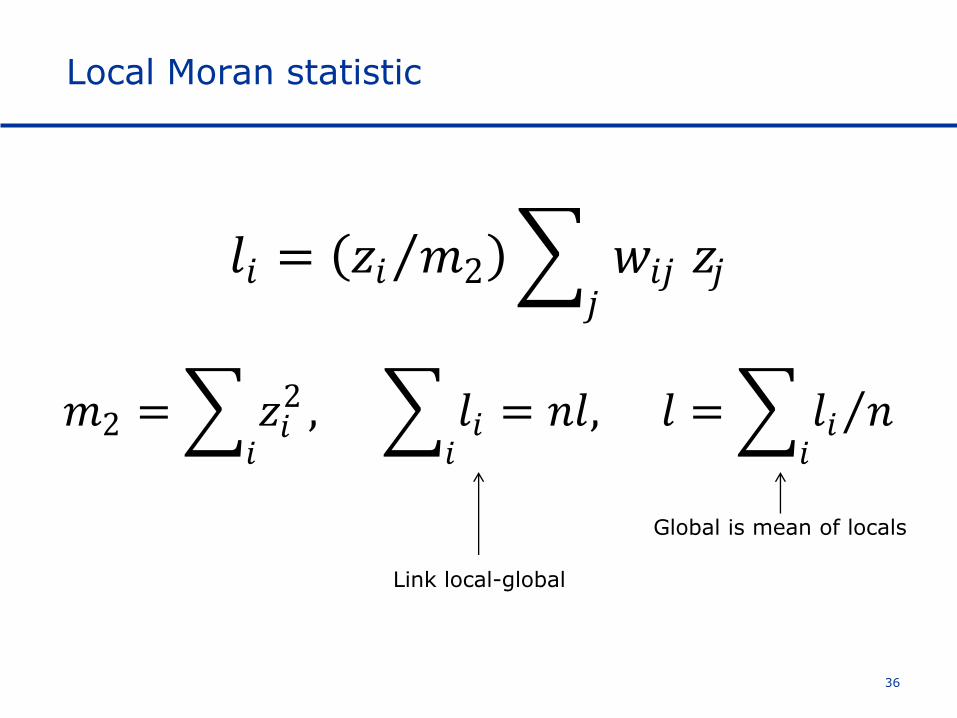
Local Moran statistic

Global is mean of locals

Link local-global

𝑙𝑖 = 𝑧𝑖 𝑚2 𝑤𝑖𝑗𝑗

𝑧𝑗

𝑚2 = 𝑧𝑖2

𝑖, 𝑙𝑖

𝑖= 𝑛𝑙, 𝑙 = 𝑙𝑖 𝑛

𝑖

37

Inference

Computational

Conditional permutation

Hold value at i fixed, permute others

38

LISA significance map

Locations with significant local statistics

Sensitivity analysis to p-value

Choropleth Map

Shading by significance

Non-significant locations not highlighted

39

LISA cluster map

Only the significant locations

Matches significance map

Types of spatial autocorrelation

Spatial clusters

high-high (red), low-low (blue)

Spatial outliers

high-low (light red), low-high (light blue)

40

Spatial clusters and spatial outliers

Spatial outliers

Individual locations

Spatial clusters

Core of the cluster in LISA map

Cluster itself also includes neighbors

Use p < 0.01 to identify meaningful cluster

cores and their neighbors

Conditional local cluster maps

41

Caveats

LISA clusters and hot spots

Suggest interesting locations

Suggest significant spatial structure

Do not explain

Need to account for multivariate relations

Univariate spatial autocorrelation due to other

covariates

Spatial Econometrics

42

Exercise 10 (LISA)

Compute the local Moran statistic and associated significance map and cluster map

Assess the sensitivity of the cluster map to the number of permutations and significance level

Interpret the notion of spatial cluster and spatial outlier

Data: Brazil_MR (RENDAPC); MSA (PCTBLCK, PCTBLACK); Grid100 (ZAR09, RANZAR09)

Exercise 11 (Conditional local cluster map)

The cluster maps can be incorporated in a conditional map view.

This is accomplished by selecting the Show As Conditional Map option

Data: Brazil_MR (RENDAPC, ESGT, M1SM)

43

44

Reference

The notes for this lecture were adapted from those

elaborated by Prof. Sergio Rey for the course

“Geographic Information Analysis – GPH 483/598”,

held in the Spring of 2014 at the School of

Geographical Sciences and Urban Planning at the

Arizona State University.

They also relied on previous material prepared by

Prof. Eduardo Haddad for the course “Regional and

Urban Economics”, held yearly at the Department of

Economics at the University of Sao Paulo.