lecture 3: multivariate regression - arizona state universitygasweete/crj604/slides/lecture...

Lecture 3: Multivariate

Regression

Homework review

Question C2.4 ask you to estimate a simple bivariate regression using IQ to predict wages.

In Stata this looks like

. reg wage IQ

not

. reg IQ wage

What does the latter command give you?

Homework review

What is the predicted increase in monthly salary for a 15 point increase in IQ?

Common mistake: 8.3*15 + 117 Why is this wrong?

What is the predicted monthly salary for IQs of 100, 115, 145?

Explaining State Homicide

Rates, cont.

Two weeks ago, we modeled state homicide rates as being dependent on one variable: poverty. In reality, we know that state homicide rates depend on numerous variables.

Our estimation of homicide rates using multiple regression will look something like this:

This allows us to estimate the “effect” of any one factor while holding “all else constant.”

0 1 1 2 2i i i k ik iY X X X


Rates, cont.

The “true” model:

Our estimation model:

0 1 1 2 2

0

1

0 1 1 2 2

0

1

i i i p ip i

p

j ij i

j

i i i k ik i

k

j ij i

j

Y E E E R

E R

Y X X X

X


Rates, cont.

Usually, the independent variables in

our estimation model are some subset

of the “true” model.

We can rewrite the “true” model in

terms of k observed and p-k

unobserved variables:

0

1 1

pk

i j ij j ij i

j j k

Y X E R


Rates, cont.

Re-arranging the “true” equation:

Re-arranging the estimation equation:

And substituting:

0

1 1

( )pk

j ij i j ij i

j j k

X Y E R

0

1

0 0

1

0 0

1

( )

k

i i j ij

j

p

i i i j ij i

j k

p

j ij i

j k

Y X

Y Y E R

E R


Rates, cont.

This means that the error term in a regression

reflects both the random component in the

dependent variable, and the impact of all excluded

variables.

Variables besides poverty thought to influence

homicide rates:

Region, high school graduation, incarceration,

unemployment, gun ownership, female headed

households, population heterogeneity, income, welfare,

law enforcement officers, IQ, smokers, other crime


Rates, example

Recall, in a bivariate regression, we found the

following:

Download multivariate homicide rate data

“murder_multi.dta” from

www.public.asu.edu/~gasweete/crj604/data/

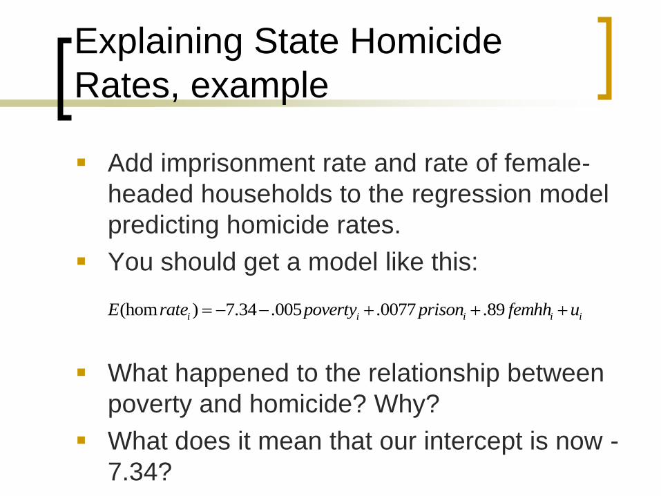
Adding imprisonment rate and rate of female-

headed households to the model yields the

following:

(hom ) 7.34 .005 .0077 .89i i i i iE rate poverty prison femhh u

(hom ) .973 .475i i iE rate poverty u

http://www.public.asu.edu/~gasweete/crj604/data/


Rates, example

Add imprisonment rate and rate of female-

headed households to the regression model

predicting homicide rates.

You should get a model like this:

What happened to the relationship between

poverty and homicide? Why?

What does it mean that our intercept is now -

7.34?



Rates, example

Of the three predictors in our model, which is

the “strongest”?

Poverty is no longer statistically significant.

How precise is our estimate of the poverty

effect? Hint: what is the 95% confidence

interval?

Does this interval contain large effects. Another

hint: what is the 95% confidence interval for the

standardized coefficient?



Rates, example

In the bivariate regression, imprisonment

rates and rates of female-headed households

were in the error term, and assumed to be

uncorrelated with poverty rates.

This assumption was false. In fact, explicitly

controlling for just these two variables

reduces the estimate for the effect of poverty

on homicide rates from .475 to -.005


Rates, example

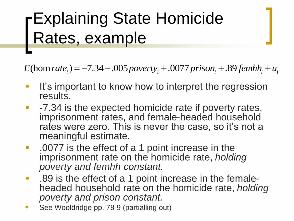
It’s important to know how to interpret the regression results.

-7.34 is the expected homicide rate if poverty rates, imprisonment rates, and female-headed household rates were zero. This is never the case, so it’s not a meaningful estimate.

.0077 is the effect of a 1 point increase in the imprisonment rate on the homicide rate, holding poverty and femhh constant.

.89 is the effect of a 1 point increase in the female-headed household rate on the homicide rate, holding poverty and prison constant.

See Wooldridge pp. 78-9 (partialling out)



Rates, example

Is the effect of female-headed households 115 times

bigger than the effect of the imprisonment rate?

prison: mean=404, s.d.=141

femhh: mean=10.2, s.d.=1.4

Because the standard deviation of prison is 100 times

larger than femhh, it’s not easy to directly compare the

two estimates, unless we calculate standardized

effects:

prison: .422, femhh: .499



Rates, example

The fitted value (or predicted value) for each

state is the expected homicide rate given the

poverty, imprisonment and female-headed

household rate.

For Arizona:


(hom ) 7.34 .005*15.2 .0077*529 .89*10.06

7.34 .076 4.07 8.95

5.60

iE rate


Rates, example

The actual homicide rate in Arizona was 7.5, so the residual is 1.9

That’s just one of 50 residuals. The sum of all residuals is zero.

The sum of the squares of all residuals is as small as possible. That’s how the estimates are chosen


ˆ 7.5 5.6 1.9i i iu y y


Rates, example

Rather than calculating the predicted values and residuals “by hand”, you can have Stata do it:

For predicted values, after your regression model (“homhat” is the name of the new variable. It can be anything you want to call it.):

For residuals (again, “resid” can be anything):


Rates, example

You can also estimate predicted values for hypothetical cases.

For example, if we wanted to look at the “average state”:


Rates, example


Rates, example

We can also look at a more disadvantaged hypothetical state:

Or an unusual state, where poverty and imprisonment rates are low but female headed household rate is high:

Is this last prediction reasonable?


Rates, example 8

10

12

14

fem

_hh

5 10 15 20poverty

?

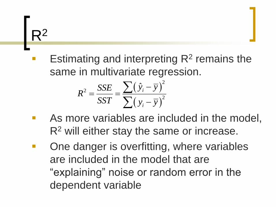
R2

Estimating and interpreting R2 remains the

same in multivariate regression.

As more variables are included in the model,

R2 will either stay the same or increase.

One danger is overfitting, where variables

are included in the model that are

“explaining” noise or random error in the

dependent variable

2

2

2

ˆi

i

y ySSER

SST y y

R2, example

. reg hom pov

Source | SS df MS Number of obs = 50

-------------+------------------------------ F( 1, 48) = 21.36

Model | 100.175656 1 100.175656 Prob > F = 0.0000

Residual | 225.109343 48 4.68977798 R-squared = 0.3080

-------------+------------------------------ Adj R-squared = 0.2935

Total | 325.284999 49 6.63846936 Root MSE = 2.1656

------------------------------------------------------------------------------

homrate | Coef. Std. Err. t P>|t| [95% Conf. Interval]

-------------+----------------------------------------------------------------

poverty | .475025 .1027807 4.62 0.000 .2683706 .6816795

_cons | -.9730529 1.279803 -0.76 0.451 -3.54627 1.600164

------------------------------------------------------------------------------

R2, example

. reg homrate pov IQ gdp leo welfare smokers income het gunowner fem_ unemp prison gradrate

pop65

Source | SS df MS Number of obs = 50

-------------+------------------------------ F( 14, 35) = 7.57

Model | 244.511494 14 17.4651067 Prob > F = 0.0000

Residual | 80.7735048 35 2.30781442 R-squared = 0.7517

-------------+------------------------------ Adj R-squared = 0.6524

Total | 325.284999 49 6.63846936 Root MSE = 1.5191

------------------------------------------------------------------------------

homrate | Coef. Std. Err. t P>|t| [95% Conf. Interval]

-------------+----------------------------------------------------------------

poverty | -.1260969 .1570399 -0.80 0.427 -.444905 .1927111

IQ | -.2960415 .2012222 -1.47 0.150 -.7045442 .1124613

gdp_percap | -.0000843 .0000675 -1.25 0.220 -.0002214 .0000527

leo | .0078023 .0062672 1.24 0.221 -.0049209 .0205255

welfare | .0043498 .0046595 0.93 0.357 -.0051096 .0138091

smokers | .0731863 .0906833 0.81 0.425 -.1109106 .2572833

income_per~p | .0000533 .0001005 0.53 0.599 -.0001508 .0002574

het | 1.716118 3.287625 0.52 0.605 -4.958115 8.390351

gunowner | .0026661 .0301547 0.09 0.930 -.0585511 .0638834

fem_hh | .5857682 .2843154 2.06 0.047 .0085773 1.162959

unemp | -.2011438 .3103236 -0.65 0.521 -.8311342 .4288467

prison | .0062964 .0026771 2.35 0.024 .0008616 .0117312

gradrate | .0027544 .0408279 0.07 0.947 -.0801306 .0856394

pop65 | -.027126 .1427545 -0.19 0.850 -.316933 .2626809

_cons | 25.41856 19.8385 1.28 0.209 -14.85575 65.69286

------------------------------------------------------------------------------

R2, example

Our R2 went up to .75! We can explain 75% of the

variance in homicide rates, or can we? It could

be that our high R2 is due to overfitting.

Solutions

If you have enough cases, split your sample and build

your model on half the cases. Test it once on the

remaining cases.

If you can’t do that, avoid iterative or stepwise modeling

as it produces biased estimates.

Pay more attention to adjusted R2.

Adjusted R2

2

2 2

1

/ ( ) 11 1 (1 )

/ ( 1)

SSE SSRR

SST SST

SSR N k NR R

SST N N k

Adjusted r-squared “penalizes” our

estimate of explained variance by the

number of parameters used.

F-test

The formula for the F-statistic remains the same

in a multivariate context, we just have to adjust

the degrees of freedom depending on how many

parameters are in the model

You can use the last expression above to

calculate the F-statistic if Stata doesn’t provide it,

and all you have is R2

2

1, 2

1

1 1k N k

SSER n kkF

SSR R kN k

F-test, cont.

The F-test can be thought of as a formal test of the

significance of R2

That last line reads: “There exists j in the set of values

from 1 to k such that βj does not equal zero.” In other

words, at least one variable is statistically significant.

0 1 2

1

: 0

: [1, ] : 0

k

j

H

H j k

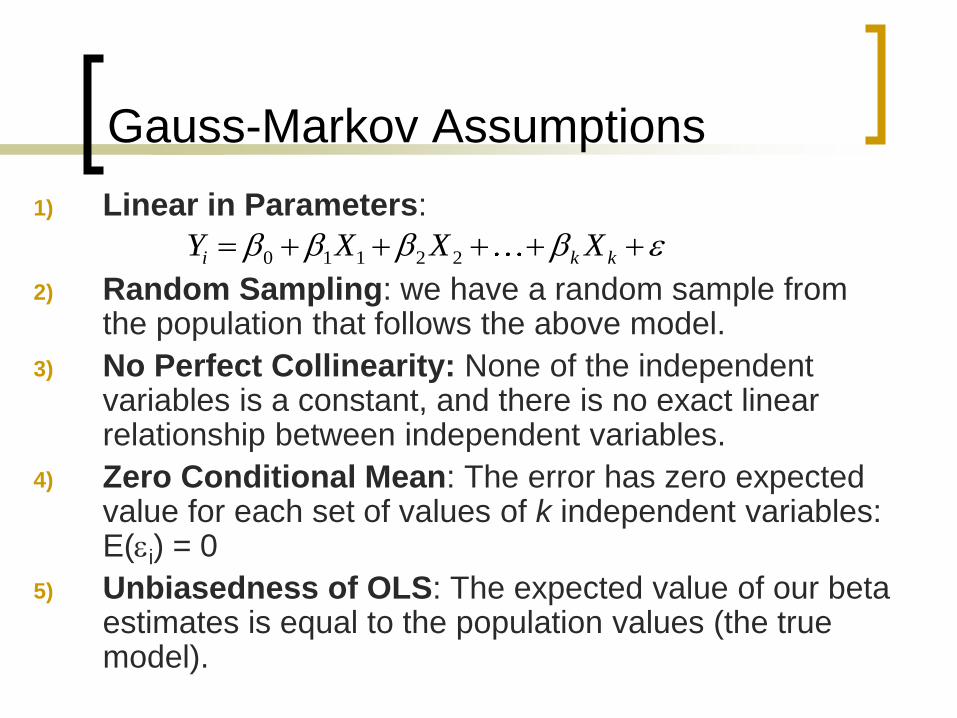
Gauss-Markov Assumptions

1) Linear in Parameters:

2) Random Sampling: we have a random sample from the population that follows the above model.

3) No Perfect Collinearity: None of the independent variables is a constant, and there is no exact linear relationship between independent variables.

4) Zero Conditional Mean: The error has zero expected value for each set of values of k independent variables: E(i) = 0

5) Unbiasedness of OLS: The expected value of our beta estimates is equal to the population values (the true model).

0 1 1 2 2i k kY X X X

Next time:

Homework: Problems 3.2, 3.4, C3.2, C3.4,

C3.6

Read: Wooldridge Chapters 3 (again) & 4

lecture 3: multivariate regression - arizona state universitygasweete/crj604/slides/lecture...

Documents