lecture 3: oligopolistic competitionmshum/ec105/matt3.pdf · introduction basic de nitions...
TRANSCRIPT

Lecture 3: Oligopolistic competition
EC 105. Industrial Organization
Mattt ShumHSS, California Institute of Technology
EC 105. Industrial Organization (Mattt Shum HSS, California Institute of Technology)Lecture 3: Oligopolistic competition 1 / 29
Outline
Outline
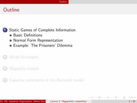
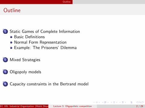
1 Static Games of Complete InformationBasic DefinitionsNormal Form RepresentationExample: The Prisoners’ Dilemma
2 Mixed Strategies
3 Oligopoly models
4 Capacity constraints in the Bertrand model
EC 105. Industrial Organization (Mattt Shum HSS, California Institute of Technology)Lecture 3: Oligopolistic competition 2 / 29

Outline
Outline
1 Static Games of Complete InformationBasic DefinitionsNormal Form RepresentationExample: The Prisoners’ Dilemma
2 Mixed Strategies
3 Oligopoly models
4 Capacity constraints in the Bertrand model
EC 105. Industrial Organization (Mattt Shum HSS, California Institute of Technology)Lecture 3: Oligopolistic competition 2 / 29
Outline
Outline
1 Static Games of Complete InformationBasic DefinitionsNormal Form RepresentationExample: The Prisoners’ Dilemma
2 Mixed Strategies
3 Oligopoly models
4 Capacity constraints in the Bertrand model
EC 105. Industrial Organization (Mattt Shum HSS, California Institute of Technology)Lecture 3: Oligopolistic competition 2 / 29
Introduction Basic Definitions
Oligopoly Models
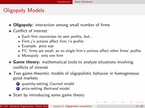
Oligopoly: interaction among small number of firms
Conflict of interest:
Each firm maximizes its own profits, but...Firm j ’s actions affect firm i ’s profitsExample: price warPC: firms are small, so no single firm’s actions affect other firms’ profitsMonopoly: only one firm
Game theory: mathematical tools to analyze situations involvingconflicts of interest
Two game-theoretic models of oligopolistic behavior in homogeneousgood markets
1 quantity-setting Cournot model2 price-setting Bertrand model
Start by introducing some game theory
EC 105. Industrial Organization (Mattt Shum HSS, California Institute of Technology)Lecture 3: Oligopolistic competition 3 / 29
Introduction Basic Definitions
Games
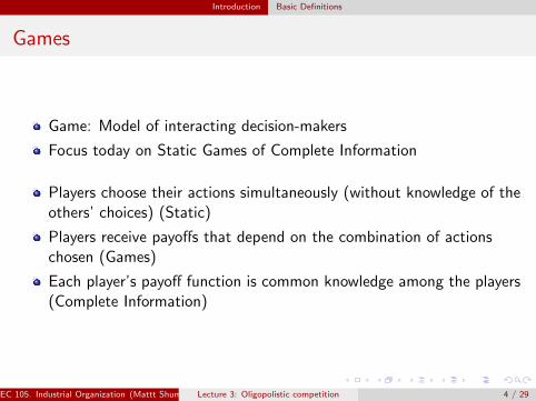
Game: Model of interacting decision-makers
Focus today on Static Games of Complete Information
Players choose their actions simultaneously (without knowledge of theothers’ choices) (Static)
Players receive payoffs that depend on the combination of actionschosen (Games)
Each player’s payoff function is common knowledge among the players(Complete Information)
EC 105. Industrial Organization (Mattt Shum HSS, California Institute of Technology)Lecture 3: Oligopolistic competition 4 / 29
Introduction Strategic Form
Normal Form Representation of Games
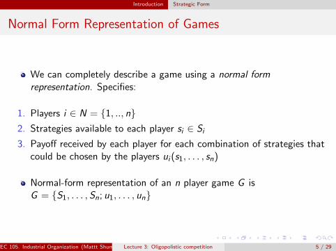
We can completely describe a game using a normal formrepresentation. Specifies:
1. Players i ∈ N = {1, .., n}2. Strategies available to each player si ∈ Si
3. Payoff received by each player for each combination of strategies thatcould be chosen by the players ui (s1, . . . , sn)
Normal-form representation of an n player game G isG = {S1, . . . ,Sn; u1, . . . , un}
EC 105. Industrial Organization (Mattt Shum HSS, California Institute of Technology)Lecture 3: Oligopolistic competition 5 / 29
Introduction Example: The Prisoners’ Dilemma
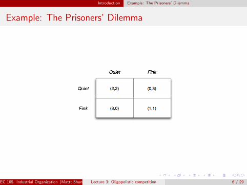
Example: The Prisoners’ Dilemma
EC 105. Industrial Organization (Mattt Shum HSS, California Institute of Technology)Lecture 3: Oligopolistic competition 6 / 29

Introduction Example: The Prisoners’ Dilemma
Nash equilibrium
A player’s best response strategy specifies the payoff-maximizing(optimal) move that should be taken in response to a set of strategiesplayed by the other players:
∀si ∈ S−i : si ∈ BR(s−i )⇔ ui (si , s−i ) ≥ ui (s′i , s−i ) ∀si ∈ Si .
A Nash Equilibrium is a profile of strategies such that each player’sstrategy is a best-response to other players’ strategies.
Definition
A strategy profile s∗ = {s∗1 , . . . , s∗n} is a Nash Equilibrium of the gameG = {S1, . . . ,Sn; u1, . . . , un} if for each player i ,
ui (s∗i , s∗−i ) ≥ ui (si , s
∗−i ) ∀si ∈ Si
In a NE: ∀i : s∗−i ∈ BR(s∗−i ). Fixed point of BR mapping.
EC 105. Industrial Organization (Mattt Shum HSS, California Institute of Technology)Lecture 3: Oligopolistic competition 7 / 29

Introduction Example: The Prisoners’ Dilemma
Nash equilibrium: Prisoner’s dilemma
What are strategies?
What is BR1(fink)? BR1(quiet)?
Why isn’t (quiet, quiet) a NE?
EC 105. Industrial Organization (Mattt Shum HSS, California Institute of Technology)Lecture 3: Oligopolistic competition 8 / 29
Introduction Example: The Prisoners’ Dilemma
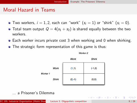
Moral Hazard in Teams
Two workers, i = 1, 2, each can “work” (si = 1) or “shirk” (si = 0).
Total team output Q = 4(s1 + s2) is shared equally between the twoworkers.
Each worker incurs private cost 3 when working and 0 when shirking.
The strategic form representation of this game is thus:
... a Prisoner’s Dilemma
EC 105. Industrial Organization (Mattt Shum HSS, California Institute of Technology)Lecture 3: Oligopolistic competition 9 / 29
Introduction Example: The Prisoners’ Dilemma
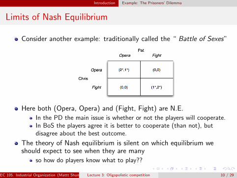
Limits of Nash Equilibrium
Consider another example: traditionally called the “ Battle of Sexes”
Here both (Opera, Opera) and (Fight, Fight) are N.E.
In the PD the main issue is whether or not the players will cooperate.In BoS the players agree it is better to cooperate (than not), butdisagree about the best outcome.
The theory of Nash equilibrium is silent on which equilibrium weshould expect to see when they are many
so how do players know what to play??
EC 105. Industrial Organization (Mattt Shum HSS, California Institute of Technology)Lecture 3: Oligopolistic competition 10 / 29

Introduction Example: The Prisoners’ Dilemma
A Coordination Game
Applications:
Conventions: which side of the road to drive on?Industry standards: VHS vs. Betamax, GSM vs. CDMA
Let’s change BoS slightly:
Now (Opera,Opera) is more desirable outcome
But the Pareto inferior outcome (Fight, Fight) is a NE
EC 105. Industrial Organization (Mattt Shum HSS, California Institute of Technology)Lecture 3: Oligopolistic competition 11 / 29
Mixed Strategies
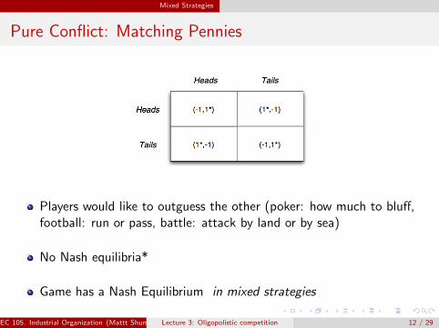
Pure Conflict: Matching Pennies
Players would like to outguess the other (poker: how much to bluff,football: run or pass, battle: attack by land or by sea)
No Nash equilibria*
Game has a Nash Equilibrium in mixed strategies
EC 105. Industrial Organization (Mattt Shum HSS, California Institute of Technology)Lecture 3: Oligopolistic competition 12 / 29

Mixed Strategies
Mixed Strategies
A mixed strategy for player i is a probability distribution over the(pure) strategies in Si .
Definition
Suppose Si = {si1, . . . , siK}. Then a mixed strategy for player i is aprobability distribution pi = {pi1, . . . , piK}, where 0 ≤ pik ≤ 1∀k and∑
k pik = 1
In Matching Pennies a mixed strategy for player i is the probabilitydistribution (q, 1− q), where q is the probability of playing Heads,1− q is the probability of playing Tails, and 0 ≤ q ≤ 1.
The mixed strategy (0, 1) is simply the pure strategy Tails, and themixed strategy (1, 0) is the pure strategy Heads.
EC 105. Industrial Organization (Mattt Shum HSS, California Institute of Technology)Lecture 3: Oligopolistic competition 13 / 29

Mixed Strategies
Nash Equilibrium in Mixed Strategies
Consider a two player game. The expected payoff of player i for amixed strategy profile p1, p2 is
vi (p1, p2) =∑j
∑k
p1jp2kui (s1j , s2k)
Definition
(p∗1 , p∗2) is a Nash equilibrium of the game G = {∆S1,∆S2; u1, u2} if and
only if each player’s equilibrium mixed strategy is a best response to theother player’s equilibrium mixed strategy:
v1(p∗1 , p∗2) ≥ v1(p1, p
∗2) ∀p1 ∈ ∆S1
andv2(p∗1 , p
∗2) ≥ v1(p∗1 , p2) ∀p2 ∈ ∆S2
EC 105. Industrial Organization (Mattt Shum HSS, California Institute of Technology)Lecture 3: Oligopolistic competition 14 / 29
Mixed Strategies
Nash Equilibrium in Mixed Strategies
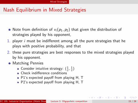
Note from definition of vi (p1, p2) that given the distribution ofstrategies played by his opponent,
1. player i must be indifferent among all the pure strategies that heplays with positive probability, and that
2. these pure strategies are best responses to the mixed strategies playedby his opponent.
Matching Pennies
Consider intuitive strategy: ( 12 ,
12 )
Check indifference conditionsP1’s expected payoff from playing H, TP2’s expected payoff from playing H, T
EC 105. Industrial Organization (Mattt Shum HSS, California Institute of Technology)Lecture 3: Oligopolistic competition 15 / 29

Mixed Strategies
Remarks
Mixed strategy idea is nice, but is it realistic?
Interpret pi not as coin flipping, but as j ’s beliefs, and i ’s beliefsabout j ’s beliefs and so on (Harsanyi)
Look for real-world evidence of mixed stategy behavior: sports!Penalty kicks in soccer
Do goalees play in a way that kickers are indifferent between kickdirections?
Service direction in tennis.
EC 105. Industrial Organization (Mattt Shum HSS, California Institute of Technology)Lecture 3: Oligopolistic competition 16 / 29

Oligopoly models
Cournot model 1
Next we apply concepts from game theory to analyze firm behavior inoligopoly.
Players: 2 identical firms
Strategies: firm 1 set q1, firm 2 sets q2
Inverse market demand curve: p = a− bQ = a− b(q1 + q2).
Constant marginal costs: C (q) = cq
Payoffs are profits, as a function of strategies:π1 = q1(a− b(q1 + q2))− cq1 = q1(a− b(q1 + q2)− c).π2 = q2(a− b(q1 + q2))− cq2 = q2(a− b(q1 + q2)− c).
EC 105. Industrial Organization (Mattt Shum HSS, California Institute of Technology)Lecture 3: Oligopolistic competition 17 / 29

Oligopoly models
Cournot model 2
Firm 1: maxq1 π1 = q1(a− b(q1 + q2)− c).
FOC: a− 2bq1 − bq2 − c = 0→ q1 = a−c2b −
q22 ≡ BR1(q2).
Similarly, BR2(q1) = a−c2b −
q12 .
Symmetric, so in a Nash equilibrium firms will produce same amountso that q1 = q2 ≡ q∗.
Symmetric NE quantity q∗ satisfies q∗ = BR1(q∗) = BR2(q∗) =⇒q∗ = a−c
3b .
Graph: NE at intersection of two firms’ BR functions.
Equilibrium price: p∗ = p(q∗) = 13a + 2
3c
Each firm’s profit: π∗ = π1 = π2 = (a−c)2
9b
Straightforward extension to N ≥ 2 firms.
EC 105. Industrial Organization (Mattt Shum HSS, California Institute of Technology)Lecture 3: Oligopolistic competition 18 / 29

Oligopoly models
Cournot model 3
Prisoner’s dilemma flavor in Nash Equilibrium of Cournot game
If firms cooperate: maxq = 2q(a− b(2q)− c)→ qj = (a−c)4b
pj = 12 (a + c), higher than p∗.
πj = (a−c)2
8b , higher than π∗.
But why can’t each firm do this? Because NE condition is notsatisfied: qj 6= BR1(qj), and qj 6= BR2(qj). Analogue of (quiet, quiet)in prisoner’s dilemma.
What if we repeat the game? Possibility of punishment for cheating.
EC 105. Industrial Organization (Mattt Shum HSS, California Institute of Technology)Lecture 3: Oligopolistic competition 19 / 29

Oligopoly models
Market power and policy implications
More generally, the Cournot problem is:
max q1π1(q1, q2) = q1P(q1 + q2)− C1(q1) (1)
with first-order condition
∂π1(q1, q2)
∂q1= P(q1 + q2)− C ′1(q1) + q1P
′(q1 + q2) = 0 (2)
This can be rearranged to yield an expression for the Cournot markup(or Lerner index):
L1 ≡P − C ′1
P=α1
εα1 = q1/Q; ε = Q ′P/Q = P/(P ′Q).
Lerner index is proportional to the firm’s market share and inverselyproportional to the elasticity of demand.
EC 105. Industrial Organization (Mattt Shum HSS, California Institute of Technology)Lecture 3: Oligopolistic competition 20 / 29
Oligopoly models
Markups and Concentration: Herfindahl index
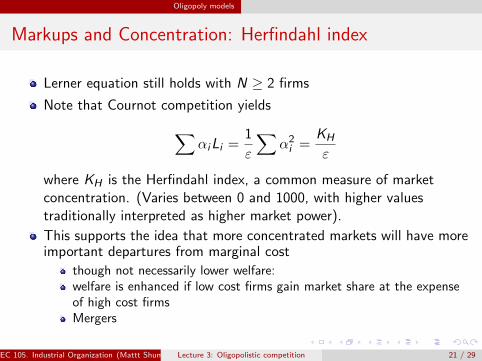
Lerner equation still holds with N ≥ 2 firms
Note that Cournot competition yields∑αiLi =
1
ε
∑α2i =
KH
ε
where KH is the Herfindahl index, a common measure of marketconcentration. (Varies between 0 and 1000, with higher valuestraditionally interpreted as higher market power).
This supports the idea that more concentrated markets will have moreimportant departures from marginal cost
though not necessarily lower welfare:welfare is enhanced if low cost firms gain market share at the expenseof high cost firmsMergers
EC 105. Industrial Organization (Mattt Shum HSS, California Institute of Technology)Lecture 3: Oligopolistic competition 21 / 29

Oligopoly models
Bertrand price-setting model
Recall: in analyzing monopoly, the outcome does not depend onwhether we view the monopoly as choosing prices or quantities.In oligopoly, this matters a lot! Consider this price-setting game.
Players: 2 identical firmsFirm 1 sets p1, firm 2 sets p2
Market demand is q = ab −
1bp. C (q) = cq.
Recall: products are homogeneous, or identical. This implies that allthe consumers will go to the firm with the lower price:
π1 =
(p1 − c)( ab −
1bp1) if p1 < p2
12 (p1 − c)( a
b −1bp1) if p1 = p2
0 if p1 > p2
(3)
Firm 1’s best response:
BR1(p2) =
{p2 − ε if p2 − ε > cc otherwise
(4)
NE: p∗ = BR1(p∗) = BR2(p∗)Unique p∗ = c! The “Bertrand paradox”.
EC 105. Industrial Organization (Mattt Shum HSS, California Institute of Technology)Lecture 3: Oligopolistic competition 22 / 29

Oligopoly models
Cournot vs. Bertrand
Recall: with homogeneous products, firms are “price takers”.Bertrand outcome coincides with competitive outcome.
Contrast with Cournot results. Presents a conundrum for policyanalysis of oligopolistic industries. Is “two enough” for competition?
Some resolutions:
Capacity constraints: one firm can’t supply the whole marketDifferentiated productsConsumer search
EC 105. Industrial Organization (Mattt Shum HSS, California Institute of Technology)Lecture 3: Oligopolistic competition 23 / 29

Capacity constraints in the Bertrand model
Capacity constraints
Now add capacity constraints to the model: k1, k2. Zero productioncosts if produce under capacity; cannot produce above.
For inverse demand P = 1− Q, assume that k1 + k2 ≤ 1.
Let R(k2) = (1− k2)/2 denote firm 1’s best response to productionof k2 by firm 2, at zero production costs. (“monopolist output onresidual demand curve”).
EC 105. Industrial Organization (Mattt Shum HSS, California Institute of Technology)Lecture 3: Oligopolistic competition 24 / 29

Capacity constraints in the Bertrand model
Case 1: small capacities
Assume capacities are small, so that k1 ≤ R(k2). Similarly,k2 ≤ R(k1)
Claim: Firms exhaust capacity, and price p∗ = 1− k1 − k2
p1 = p2 < p∗: cannot produce morep1 = p2 > p∗: at least one firm cannot sell to capacity; this firm shouldundercut slightly, and sell capacitypi < pj not feasible: either (i) firm i is capacity constrained, and willraise its price; or (ii) pi is firm i ’s monopoly price and supplies entiredemand, but then firm j is making zero profit and should undercut.
Note that p∗ is above marginal cost of zero
Suggestive: what if you “endogenize” capacity, and add on initialcapacity investment stage?
Each firm chooses ki to maximize ki (1− ki − k−i ).Symmetric solution is ???
EC 105. Industrial Organization (Mattt Shum HSS, California Institute of Technology)Lecture 3: Oligopolistic competition 25 / 29

Capacity constraints in the Bertrand model
Case 2: Large capacities
For the rest, assume k1 = k2 = k for convenience.
Now assume k > R(k). Is p = 1− 2k an equilibrium?
No– firm 1 (say) can deviate by decreasing production toq1 = R(k) < k , resulting in higher price.
Consider the following sequence of events:
EC 105. Industrial Organization (Mattt Shum HSS, California Institute of Technology)Lecture 3: Oligopolistic competition 26 / 29
Capacity constraints in the Bertrand model
Edgeworth cycles
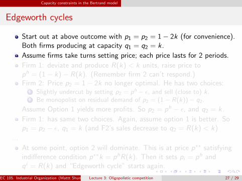
Start out at above outcome with p1 = p2 = 1− 2k (for convenience).Both firms producing at capacity q1 = q2 = k .
Assume firms take turns setting price; each price lasts for 2 periods.
Firm 1: deviate and produce R(k) < k units, raise price toph = (1− k)− R(k). (Remember firm 2 can’t respond.)Firm 2: Price p2 = 1− 2k no longer optimal. He has two choices:
1 Slightly undercut by setting p2 = ph − ε, and sell (close to) k.2 Be monopolist on residual demand of p2 = (1− R(k))− q2.
Assume Option 1 yields more profits. So p2 = ph − ε, and q2 = k .
Firm 1: has same two choices. Again, assume option 1 is better. Sop1 = p2 − ε, q1 = k (and F2’s sales decrease to q2 = R(k) < k)
...
At some point, option 2 will dominate. This is at price p∗∗ satisfyingindifference condition p∗∗k = phR(k). Then it sets pi = ph andqi = R(k) and “Edgeworth cycle” starts again.
EC 105. Industrial Organization (Mattt Shum HSS, California Institute of Technology)Lecture 3: Oligopolistic competition 27 / 29

Capacity constraints in the Bertrand model
Edgeworth cycles
Start out at above outcome with p1 = p2 = 1− 2k (for convenience).Both firms producing at capacity q1 = q2 = k .
Assume firms take turns setting price; each price lasts for 2 periods.
Firm 1: deviate and produce R(k) < k units, raise price toph = (1− k)− R(k). (Remember firm 2 can’t respond.)Firm 2: Price p2 = 1− 2k no longer optimal. He has two choices:
1 Slightly undercut by setting p2 = ph − ε, and sell (close to) k.2 Be monopolist on residual demand of p2 = (1− R(k))− q2.
Assume Option 1 yields more profits. So p2 = ph − ε, and q2 = k .
Firm 1: has same two choices. Again, assume option 1 is better. Sop1 = p2 − ε, q1 = k (and F2’s sales decrease to q2 = R(k) < k)
...
At some point, option 2 will dominate. This is at price p∗∗ satisfyingindifference condition p∗∗k = phR(k). Then it sets pi = ph andqi = R(k) and “Edgeworth cycle” starts again.
EC 105. Industrial Organization (Mattt Shum HSS, California Institute of Technology)Lecture 3: Oligopolistic competition 27 / 29

Capacity constraints in the Bertrand model
Edgeworth cycles
Not an equilibrium phenomenon. In fact, this model has nopure-strategy equilibria.
(But have mixed strategy equilibria)
Can be shown to be equilibrium path of dynamic game(Maskin-Tirole)
Fixed limited capacity is crucial.
Otherwise F1 will never raise price initiallyBc F2 will capture all the consumers
F1 “pays a price” in initial period to be the market leader
Such cycles are empirical regularity in gasoline markets:
TorontoPerth
EC 105. Industrial Organization (Mattt Shum HSS, California Institute of Technology)Lecture 3: Oligopolistic competition 28 / 29
Capacity constraints in the Bertrand model
Summary
Nash equilibrium: a strategy profile in which each player’s NEstrategy is a best-response to opponents’ best-response strategies2-player case: s1 = BR1(s2), s2 = BR2(s1)
Cournot: noncooperative quantity-choice game.
Bertrand: noncooperative price-setting game.
Bertrand paradox: when goods are homogeneous, firms are price-takers!Price competition with capacity constraints.
EC 105. Industrial Organization (Mattt Shum HSS, California Institute of Technology)Lecture 3: Oligopolistic competition 29 / 29