lecture 4: dynamic programming - · pdf filelecture 4: dynamic programming fatih guvenen...

Lecture 4: Dynamic Programming

Fatih Guvenen

January 10, 2016

Fatih Guvenen Lecture 4: Dynamic Programming January 10, 2016 1 / 30

Goal

Solve

V (k , z) = maxc,k 0

⇥u(c) + �E(V (k 0, z 0)|z)

⇤

c + k 0 = (1 + r)k + zz 0 = ⇢z + ⌘

Questions:

1 Does a solution exist?

2 Is it unique?

3 If the answers to (1) and (2) are yes: how do we find this solution?


Contraction Mapping Theorem

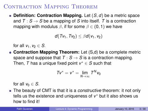
Definition: Contraction Mapping. Let (S, d) be a metric spaceand T : S ! S be a mapping of S into itself. T is a contractionmapping with modulus �, if for some � 2 (0, 1) we have

d(Tv1,Tv2) �d(v1, v2)

for all v1, v2 2 S.

Contraction Mapping Theorem: Let (S,d) be a complete metricspace and suppose that T : S ! S is a contraction mapping.Then, T has a unique fixed point v⇤ 2 S such that

Tv⇤ = v⇤ = limN!1

T Nv0

for all v0 2 S.

The beauty of CMT is that it is a constructive theorem: it not onlytells us the existence and uniqueness of v⇤ but it also shows ushow to find it!


Qualitative Properties of v⇤

We cannot apply CMT in certain cases, because the particular setwe are interested in is not a complete metric space.

The following corollary comes in handy in those cases.

Corollary: Let (S,d) be a complete metric space and T : S ! Sbe a contraction mapping with Tv⇤ = v⇤.

a. If S is a closed subset of S, and T (S) ⇢ S, then v⇤ 2 S.

b. If, in addition, T (S) ⇢ S ⇢ S, then v⇤ 2 S.

S = {continuous, bounded, strictly concave}. Not a completemetric space. S = continuous, bounded, weakly concave} is. Sowe need to be able to establish that T maps elements in S into S.


A Prototype Problem


u(c) + �

ZV (k 0, z 0)f (z 0|z)dz 0

�

c + k 0 = (1 + r)k + zz 0 = ⇢z + ⌘

CMT tells us to start with a guess V0 and then repeatedly solvethe problem in the RHS.

But:How to evaluate the conditional expectation?

I Several non-trivial issues that are easy to underestimate

How to do constrained optimization (esp. in multi-dimension)?

This course will focus on methods that are especially suitable forincomplete mkts/heterogenous agent models.


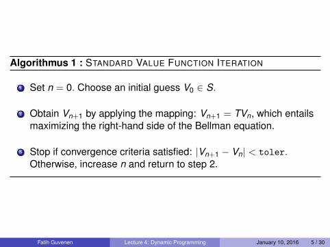
Algorithmus 1 : STANDARD VALUE FUNCTION ITERATION

1 Set n = 0. Choose an initial guess V0 2 S.

2 Obtain Vn+1 by applying the mapping: Vn+1 = TVn, which entailsmaximizing the right-hand side of the Bellman equation.

3 Stop if convergence criteria satisfied: |Vn+1 � Vn| < toler.Otherwise, increase n and return to step 2.


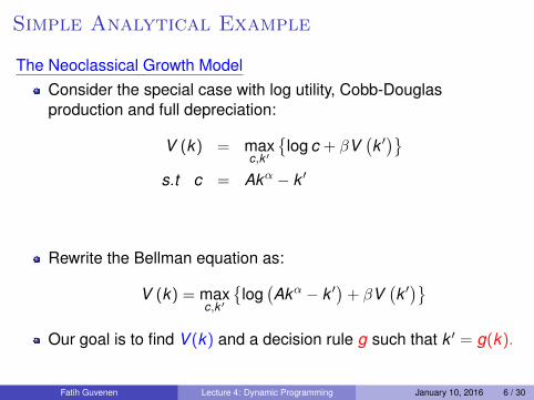
Simple Analytical Example

The Neoclassical Growth ModelConsider the special case with log utility, Cobb-Douglasproduction and full depreciation:

V (k) = maxc,k 0

�log c + �V

�k 0�

s.t c = Ak↵ � k 0

Rewrite the Bellman equation as:

V (k) = maxc,k 0

�log

�Ak↵ � k 0�+ �V

�k 0�

Our goal is to find V (k) and a decision rule g such that k 0 = g(k).


I. Backward Induction (Brute Force)

If t = T < 1, in the last period we would have: V0 (k) ⌘ 0 for all k .Therefore:

V1 (k) = maxk 0

8><

>:log

�Ak↵ � k 0�+ �V0

�k 0�

| {z }⌘0

9>=

>;

V1 = maxk 0 log (Ak↵ � k 0) ) k 0 = 0 ) V1 (k) = log A + ↵ log k

Substitute V1 into the RHS of V2 :

V2 = maxk 0

�log

�Ak↵ � k 0�+ �

�log A + ↵ log k 0�

) FOC :1

Ak↵ � k 0 =�↵

k 0 ) k 0 =↵�Ak↵

1 + ↵�

Substitute k 0 to obtain V2. We can keep iterating to find thesolution.


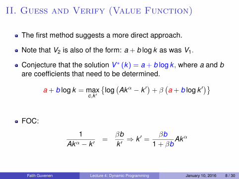
II. Guess and Verify (Value Function)

The first method suggests a more direct approach.

Note that V2 is also of the form: a + b log k as was V1.

Conjecture that the solution V ⇤ (k) = a + b log k , where a and bare coefficients that need to be determined.

a + b log k = maxc,k 0

�log

�Ak↵ � k 0�+ �

�a + b log k 0�

FOC:

1Ak↵ � k 0 =

�bk 0 ) k 0 =

�b1 + �b

Ak↵


II. Guess and Verify (Value Function)

Let LHS = a + b log k . Plug in the expression for k 0 into the RHS:

RHS = log✓

Ak↵ � �b1 + �b

Ak↵

◆+ �

✓a + b log

✓�b

1 + �bAk↵

◆◆

= (1 + �b) log A + log✓

11 + �b

◆+ a� + b� log

✓�b

1 + �b

◆

+↵ (1 + �b) log k

Imposing the condition that LHS ⌘ RHS for allk , we find a and b :

a =1

1 � �

11 � ↵�

log A + (1 � ↵�) log (1 � ↵�)

+↵� log↵�

�

b =↵

1 � ↵�

We have solved the model!Fatih Guvenen Lecture 4: Dynamic Programming January 10, 2016 9 / 30

Guess and Verify as a Numerical Tool

Although this was a very special example, the same logic can beused for numerical analysis.

As long as the true value function is “well-behaved” (smooth, etc),we can choose a sufficiently flexible functional form that has afinite (ideally small) number of parameters.

Then we can apply the same logic as above and solve for theunknown coefficients, which then gives us the complete solution.

Many solution methods rely on various version of this general idea(perturbation methods, collocation methods, parametrizedexpectations)


III. Guess and Verify (Policy Functions)a.k.a Euler equations approach

Let the policy rule for savings be: k 0 = g(k). The Euler equation is:

1Ak↵ � g (k)

��↵A

⇣g (k)↵�1

⌘

A (g (k)↵ � g (g (k)))= 0 for all k .

which is a functional equation in g (k) .

Guess g (k) = sAk↵, and substitute above:

1(1 � s)Ak↵

=�↵A (sAk↵)↵�1

A ((sAk↵)↵ � sA (aAk↵)↵)

As can be seen, k cancels out, and we get s = ↵�.

By using a very flexible choice of g() this method too can be usedfor solving very general models.


Back to VFI

VFI can be very slow when � ⇡ 1. Three ways to accelerate.

1 (Howard’s) Policy Iteration Algorithm (together with its “modified”version)

2 MacQueen-Porteus (MQP) error bounds

3 Endogenous Grid Method (EGM).

In general, basic VFI should never be used without at least one ofthese add-ons.

I EGM is your best bet when it’s applicable. But in certain cases, it’snot.

I In those cases, a combination of Howard’s algorithm and MQP canbe very useful.


Howard’s Policy IterationConsider the neoclassical growth model:


⇢c1��

1 � �+ �E

�V�k 0, z 0� |z

��

s.t c + k 0 = ezk↵ + (1 � �)k (P1)z 0 = ⇢z + ⌘0, k 0 � k .

In stage n of the VFI algorithm, solve for the policy rule:

sn(k , z) = arg maxs�k

((ezj k↵

i + (1 � �)k � s)1��

1 � �+ �E

�Vn

�s, z 0� |z

�).

(1)

The second step isVn+1 = TsnVn. (2)


Policy Iteration

Maximization step can be very time consuming. So it seems like awaste that we use the new policy only one period in updating toVn+1.

I A simple but key insight is that (2) is also a contraction withmodulus �. Therefore if we were to repeatedly apply Tsn , it wouldalso converge to a fixed point itself at rate �.

I Of course, this fixed point would not be the solution of the originalBellman equation we would like to solve.

I But it is an operatore that is much cheaper to apply. So we maywant to apply it more than once.


Two Properties of Howard’s Algorithm

Puterman and Brumelle (1979) show that:

Policy iteration is equivalent to Newton’s method applied todynamic programming.

Thus, just like Newton’s method it has two properties:

1 it is guaranteed to converge to the true solution when the initialpoint, V0, is in the domain of attraction of V ⇤, and

2 when (i) is satisfied, it converges at a quadratic rate in iterationindex n.

Bad news: no more global convergence like VFI (unless statespace is discrete)

Good news: potentially very fast convergence.


Algorithmus 2 : VFI WITH POLICY ITERATION ALGORITHM

1 Set n = 0. Choose an initial guess v0 2 S.

2 Obtain sn as in (1) and take the updated value function to be:vn+1 = limm!1 T m

snvn, which is the (fixed point) value function

resulting from using policy, sn, forever.1

3 Stop if convergence criteria satisfied: |vn+1 � vn| < toler.Otherwise, increase n and return to step 1.


Modified Policy Iteration

Quadratic convergence is a bit misleading: this is the rate in n.

And in contrast to VFI, Howard’s algorithm takes a lot of time toevaluate step 2.

So overall, it may not be much faster when the state space islarge.

Second, the basin of attraction can be small.

These can be fixed by slightly modifying the algorithm.


Error Bounds: Background

In iterative numerical algorithms, we need a stopping rule.

In dynamic programming we want to know how far we are from thetrue solution in each iteration.

Contraction mapping theorem can be used to show:

kv⇤ � vkk1 11 � �

kvk+1 � vkk1 .

So if we want to stop when we are " away from true solution,kvk+1 � vkk1 < "⇥ (1 � �).


Algorithmus 3 : VFI WITH Modified POLICY IMPROVEMENT ALGO-RITHM

1 Modify Step 2 of Howard’s algorithm: Obtain sn as in (1) and takethe updated value function to be: vn+1 = T m

snvn, which entails m

applications of Howard’s mapping to update to vn+1.


Error Bounds: Background

Remarks:1 This bound is for the worst case scenario (sup-norm). If v⇤ varies

over a wide range, this bound may be misleading.

I Consider u(c) = c�10

�10 . Typically, v will cover an enormous range ofvalues. Bound might be too pessimistic.

2 ASIDE: In general, it may be hard to judge what an " deviation in vmeans in economic terms.

I Another approach will be to define stopping rule in the policy space.It is easier to judge what it means to consume x% less thanoptimal.

I Typically policies converge faster than values so this might allowstopping sooner.


MacQueen-Porteus Bounds

Theorem

[MacQueen-Porteus bounds] Consider

V (xi) = maxy2�(xi )

2

4U(xi , y) + �JX

j=1

⇡ij(y)V (xj)

3

5 , (3)

define

cn =�

1 � �⇥ min [Vn � Vn�1] cn =

�

1 � �⇥ max [Vn � Vn�1] (4)

Then, for all x 2 X, we have:

T nV0(x) + cn V ⇤(x) T nV0(x) + cn. (5)

Furthermore, with each iteration, the two bounds approach the truesolution monotonically.


MQP Bounds: Comments

MQP bounds can be quite tight.Example: Vn(x)� Vn�1(x) = ↵ for all x . Suppose ↵ = 100 (alarge number).The usual bound implies:kV ⇤ � Vnk1 1

1�� kVn(x)� Vn�1(x)k1 = ↵1�� , so we would keep

iterating.MQP implies cn = cn = ↵, which the then implies

↵�

1 � �= V ⇤(x)� T nV0(x) =

↵�

1 � �.

We find V ⇤(x) = Vn(x) + ↵�1�� , in one step!

MQP: both lower and upper bound for signed difference. No upperbound only for sup-norm.


Algorithmus 4 : VFI WITH MACQUEEN-PORTEUS ERROR BOUNDS

[Step 2’:] Stop when cn � cn < toler. Then take the final estimate ofV ⇤ to be either the median

V = T nV0 +

✓cn + cn

2

◆

or the mean (i.e., average error bound across states):

V = T nV0 +�

n(1 � �)

nX

i=1

⇣T nV0(xi)� T n�1V0(xi)

⌘.


MQP: Convergence Rate

Bertsekas (1987) derives the convergence rate of MQP boundsalgorithm

It is proportional to the subdominant eigenvalue of ⇡ij(y⇤) (thetransition matrix evaluated at optimal policy).

VFI is proportional to the dominant eigenvalue, which is always 1.Multiplied by �, gives convergence rate.

Subdominant (2nd largest) eigenvalue (|�2|) can be much lower ornot:

I AR(1) process, discretized: |�2| = ⇢ (persistence parameter)I More than 1 ergodic set: |�2| = 1.

When persistence is low, this can lead to substantialimprovements in speed.


Endogenous Grid Method

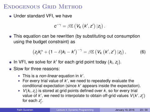
Endogenous Grid Method

Under standard VFI, we have

c�� = �E�Vk

�k 0, z 0� |zj

�.

This equation can be rewritten (by substituting out consumptionusing the budget constraint) as

�zjk↵

i + (1 � �)ki � k 0��= �E

�Vk

�k 0, z 0� |zj

�, (6)

In VFI, we solve for k 0 for each grid point today (ki , zj).

Slow for three reasons:I This is a non-linear equation in k 0.I For every trial value of k 0, we need to repeatedly evaluate the

conditional expectation (since k 0 appears inside the expectation).I V (ki , zj) is stored at grid points defined over k , so for every trial

value of k 0, we need to interpolate to obtain off-grid values V (k 0, z 0j )

for each z 0j .


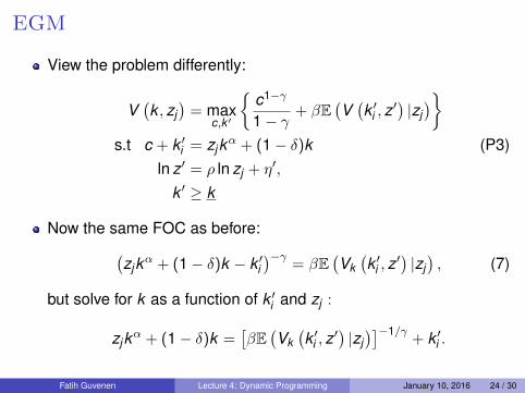
EGM

View the problem differently:

V�k , zj

�= max

c,k 0

⇢c1��

1 � �+ �E

�V�k 0

i , z0� |zj

��

s.t c + k 0i = zjk↵ + (1 � �)k (P3)

ln z 0 = ⇢ ln zj + ⌘0,

k 0 � k

Now the same FOC as before:�zjk↵ + (1 � �)k � k 0

i��

= �E�Vk

�k 0

i , z0� |zj

�, (7)

but solve for k as a function of k 0i and zj :

zjk↵ + (1 � �)k =⇥�E

�Vk

�k 0

i , z0� |zj

�⇤�1/�+ k 0

i .


EGM

Define

Y ⌘ zk↵ + (1 � �)k (8)

and rewrite the Bellman equation as:

V (Y , z) = maxk 0

((Y � k 0)1��

1 � �+ �E

�V�Y 0, z 0� |zj

�)

s.t ln z 0 = ⇢ ln zj + ⌘0.

The key observation is that Y 0 is only a function of k 0i and z 0, so we can

write the conditional expectation on the right hand side as:

V(k 0i , zj) ⌘ �E

�V�Y 0(k 0

i , z0), z 0� |zj

�.


EGM

V (Y , z) = maxk 0

((Y � k 0)1��

1 � �+ V(k 0

i , zj)

)

Now the FOC of this new problem becomes:

c⇤(k 0i , zj)

�� = Vk 0(k 0i , zj). (9)

Having obtained c⇤(k 0i , zj) from this expression, we use the resource

constraint to compute today’s end-of-period resourcesY ⇤(k 0

i , zj) = c⇤(k 0i , zj) + k 0

i as well as

V�Y ⇤(k 0

i , zj), zj�=

�c⇤(k 0

i , zj)�1��

1 � �+ V(k 0

i , zj)


EGM: The Algorithm

0: Set n = 0. Construct a grid for tomorrow’s capital and today’sshock: (k 0

i , zj). Choose an initial guess V0(k 0i , zj).

1: For all i , j , obtain

c⇤(k 0i , zj) =

�Vn

k (k0i , zj)

��1/�.

2: Obtain today’s end-of-period resources as a function oftomorrow’s capital and today’s shock:

Y ⇤(k 0i , zj) = c⇤(k 0

i , zj) + k 0i ,

and today’s updated value function,

Vn+1 �Y ⇤(k 0i , zj), zj

�=

�c⇤(k 0

i , zj)�1��

1 � �+ Vn(k 0

i , zj)

by plugging in consumption decision into the RHS.


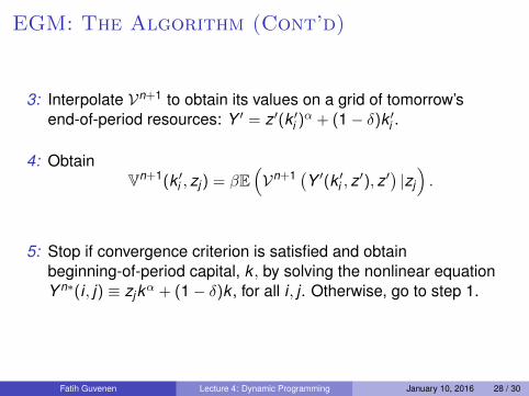
EGM: The Algorithm (Cont’d)

3: Interpolate Vn+1 to obtain its values on a grid of tomorrow’send-of-period resources: Y 0 = z 0(k 0

i )↵ + (1 � �)k 0

i .

4: ObtainVn+1(k 0

i , zj) = �E⇣Vn+1 �Y 0(k 0

i , z0), z 0� |zj

⌘.

5: Stop if convergence criterion is satisfied and obtainbeginning-of-period capital, k , by solving the nonlinear equationY n⇤(i , j) ⌘ zjk↵ + (1 � �)k , for all i , j . Otherwise, go to step 1.


Is This Worth the Trouble?

�RRA Utility 0.95 0.98 0.99 0.995

2 CRRA 28.9 74 119 247CRRA+PI 7.17 18.2 29.5 53CRRA+PI+MP 7.17 16.5 26 38CRRA+PI+MP+100grid 2.15 5.2 8.2 12Endog Grid (grid curv=2) 0.38 0.94 1.92 4

Table: Time for convergence (seconds) : dim k=300, ✓ = 3.0


Another Benchmark

� ! 0.95 0.99 0.999

MQP#

/Nmax ! 0 50 500 0 50 500 0 50 500� = 1

no 14.99 1.07 1.00 26.48 1.28 1.00 33.29 1.41 1.00yes 0.32 0.60 0.79 0.10 0.23 0.27 0.01 0.03 0.04

� = 5no 13.03 0.96 1.00 26.77 1.28 1.00 33.37 1.45 1.00yes 0.67 0.67 0.69 0.14 0.24 0.30 0.02 0.04 0.06

Table: Mc-Queen Porteus Bounds and Policy Iteration


lecture 4: dynamic programming - · pdf filelecture 4: dynamic programming fatih guvenen...

Documents