lecture 4 gaussian mixture models...

Lecture 4

Gaussian Mixture Models (GMMs)

Yossi Keshet

Based on the slides of Michael Picheny, Bhuvana Ramabhadran, and Stanley F.

Chen presented at the speech recognition course e6870 given at Colombia

University Fall 2012.

Where Are We?

Can extract features over time (LPC, MFCC, PLP) that . . .Characterize info in speech signal in compact form.Every ⇠10 ms, process window of samples . . .To get ⇠40 features.

DTW computes distance between feature vectors . . .While accounting for nonlinear time alignment.

Learned basic concepts (e.g., distances, shortest paths) . . .That will reappear throughout course.

3 / 113

DTW Revisited

w⇤ = arg minw2vocab

distance(A0test, A0

w)

Training: collect audio Aw for each word w in vocab.Generate features ) A0

w (template for w).Test time: given audio Atest, convert to A0

test.For each w , compute distance(A0

test, A0w) using DTW.

Return w with smallest distance.

4 / 113

What are Pros and Cons of DTW?

5 / 113

Pros

Easy to implement.Lots of freedom — can model arbitrary time warpings.

6 / 113

Cons: It’s Ad Hoc

Distance measures completely heuristic.Why Euclidean?Weight all dimensions of feature vector equally?

Warping paths heuristic.Too much freedom not good for robustness?Allowable local paths hand-derived.

No guarantees of optimality or convergence.

7 / 113

Cons (cont’d)

Doesn’t scale well?Run DTW for each template in training data.What if large vocabulary? Lots of templates per word?

Generalization.Doesn’t support mix and match between templates.

8 / 113

Can We Do Better?

Key insight 1: Learn as much as possible from data.e.g., distance measure; graph weights; graphstructure?

Key insight 2: Use probabilistic modeling.Use well-described theories and models from . . .Probability, statistics, and computer science . . .Rather than arbitrary heuristics with ill-definedproperties.

9 / 113

Next Two Main Topics

Gaussian Mixture models (today) — A probabilistic modelof . . .

Feature vectors associated with a speech sound.Principled distance between test frame . . .And set of template frames.

Hidden Markov models (next week) — A probabilistic modelof . . .

Time evolution of feature vectors for a speech sound.Principled generalization of DTW.

10 / 113

Part I

Gaussian Distributions

11 / 113

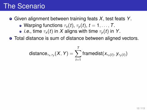
The Scenario

Given alignment between training feats X , test feats Y .Warping functions ⌧x(t), ⌧y(t), t = 1, . . . , T .i.e., time ⌧x(t) in X aligns with time ⌧y(t) in Y .

Total distance is sum of distance between aligned vectors.

distance⌧x ,⌧y (X , Y ) =TX

t=1

framedist(x⌧x (t), y⌧y (t))

12 / 113

The Scenario

Computing frame distance for pair of frames is easy.


Imagine 2d feature vectors instead of 40d for visualization.

13 / 113

Problem Formulation

What if instead of one training sample, have many?

framedist((x1⌧x1 (t), x2

⌧x2 (t), x3⌧x3 (t), . . .); y⌧y (t))

14 / 113

Ideas

Average training samples; compute Euclidean distance.Find best match over all training samples.Make probabilistic model of training samples.

15 / 113

Probabilistic Modeling

Old paradigm:


distance(A0test, A0

w)

New paradigm:


� log P(A0test|w)

P(A0|w) is (relative) frequency with which w . . .Is realized as feature vector A0.

16 / 113

Why Probabilistic Modeling?

If can estimate P(A0|w) perfectly . . .Can perform classification optimally!

e.g., two-class classification (w/ classes equally frequent)Choose yes iff P(A0

test|yes) > P(A0test|no).

This is best you can do!

17 / 113

Why Probabilistic Modeling?

In limit of infinite data, . . .Can estimate probabilities perfectly (consistency ).

In real world situations (e.g., sparse data) . . .No guarantees.Still, better to follow principles imperfectly . . .Than to not have principles at all.

18 / 113

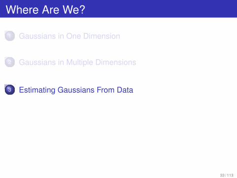
Where Are We?

1 Gaussians in One Dimension

2 Gaussians in Multiple Dimensions

3 Estimating Gaussians From Data

19 / 113

Problem Formulation, Two Dimensions

Estimate P(x1, x2), the “frequency” . . .That training sample occurs at location (x1, x2).

20 / 113

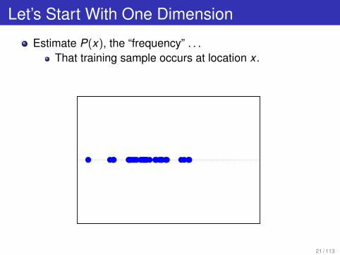
Let’s Start With One Dimension

Estimate P(x), the “frequency” . . .That training sample occurs at location x .

21 / 113

The Gaussian or Normal Distribution

Pµ,�2(x) = N (µ, �2) =1p2⇡�

e�(x�µ)2

2�2

Parametric distribution with two parameters:µ = mean (the center of the data).�2 = variance (how wide data is spread).

22 / 113

Visualization

Density function:

µ� 4� µ� 2� µ µ + 2� µ + 4�

Sample from distribution:

µ� 4� µ� 2� µ µ + 2� µ + 4�

23 / 113

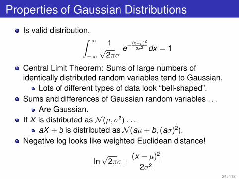
Properties of Gaussian Distributions

Is valid distribution.Z 1

�1

1p2⇡�

e�(x�µ)2

2�2 dx = 1

Central Limit Theorem: Sums of large numbers ofidentically distributed random variables tend to Gaussian.

Lots of different types of data look “bell-shaped”.Sums and differences of Gaussian random variables . . .

Are Gaussian.If X is distributed as N (µ, �2) . . .

aX + b is distributed as N (aµ + b, (a�)2).Negative log looks like weighted Euclidean distance!

lnp

2⇡� +(x � µ)2

2�2

24 / 113

Where Are We?




25 / 113

Gaussians in Two Dimensions

N (µ1, µ2, �21, �

22) =

12⇡�1�2

p1� r 2

e� 1

2(1�r2)

„(x1�µ1)2

�21

� 2rx1x2�1�2

+(x2�µ2)2

�22

«

If r = 0, simplifies to

1p2⇡�1

e� (x1�µ1)2

2�21

1p2⇡�2

e� (x2�µ2)2

2�22 = N (µ1, �

21)N (µ2, �

22)

i.e., like generating each dimension independently.

26 / 113

Example: r = 0, �1 = �2

x1, x2 uncorrelated.Knowing x1 tells you nothing about x2.

27 / 113

Example: r = 0, �1 6= �2

x1, x2 can be uncorrelated and have unequal variance.

28 / 113

Example: r > 0, �1 6= �2

x1, x2 correlated.Knowing x1 tells you something about x2.

29 / 113

Generalizing to More Dimensions

If we write following matrix:

⌃ =

��2

1 r�1�2r�1�2 �2

2

��

then another way to write two-dimensional Gaussian is:

N (µ,⌃) =1

(2⇡)d/2|⌃|1/2 e�12 (x�µ)T ⌃�1(x�µ)

where x = (x1, x2), µ = (µ1, µ2).More generally, µ and ⌃ can have arbitrary numbers ofcomponents.

Multivariate Gaussians.

30 / 113

Diagonal and Full Covariance Gaussians

Let’s say have 40d feature vector.How many parameters in covariance matrix ⌃?The more parameters, . . .The more data you need to estimate them.

In ASR, usually assume ⌃ is diagonal ) d params.This is why like having uncorrelated features!

(Research direction: is there something in between?)

31 / 113

Computing Gaussian Log Likelihoods

Why log likelihoods?Full covariance:

log P(x) = �d2

ln(2⇡)� 12

ln |⌃|� 12

(x� µ)T⌃�1(x� µ)

Diagonal covariance:

log P(x) = �d2

ln(2⇡)�dX

i=1

ln �i �12

dX

i=1

(xi � µi)2/�2

i

Again, note similarity to weighted Euclidean distance.Terms on left independent of x; precompute.A few multiplies/adds per dimension.

32 / 113

Where Are We?




33 / 113

Estimating Gaussians

Give training data, how to choose parameters µ, ⌃?Find parameters so that resulting distribution . . .

“Matches” data as well as possible.Sample data: height, weight of baseball players.

140

180

220

260

300

66 70 74 78 8234 / 113

Maximum-Likelihood Estimation (Univariate)

One criterion: data “matches” distribution well . . .If distribution assigns high likelihood to data.

Likelihood of string of observations x1, x2, . . . , xN is . . .Product of individual likelihoods.

L(xN1 |µ, �) =

NY

i=1

1p2⇡�

e�(xi�µ)2

2�2

Maximum likelihood estimation: choose µ, � . . .That maximizes likelihood of training data.

(µ, �)MLE = arg maxµ,�

L(xN1 |µ, �)

35 / 113

Why Maximum-Likelihood Estimation?

Assume we have “correct” model form.Then, in presence of infinite training samples . . .

ML estimates approach “true” parameter values.For most models, MLE is asymptotically consistent,unbiased, and efficient.

ML estimation is easy for many types of models.Count and normalize!

36 / 113

What is ML Estimate for Gaussians?

Much easier to work with log likelihood L = lnL:

L(xN1 |µ, �) = �N

2ln 2⇡�2 � 1

2

NX

i=1

(xi � µ)2

�2

Take partial derivatives w.r.t. µ, �:

@L(xN1 |µ, �)

@µ=

NX

i=1

(xi � µ)

�2

@L(xN1 |µ, �)

@�2 = � N2�2 +

NX

i=1

(xi � µ)2

�4

Set equal to zero; solve for µ, �2.

µ =1N

NX

i=1

xi �2 =1N

NX

i=1

(xi � µ)2

37 / 113

What is ML Estimate for Gaussians?

Multivariate case.

µ =1N

NX

i=1

xi

⌃ =1N

NX

i=1

(xi � µ)T (xi � µ)

What if diagonal covariance?Estimate params for each dimension independently.

38 / 113

Example: ML Estimation

Heights (in.) and weights (lb.) of 1033 pro baseball players.Noise added to hide discretization effects.

⇠stanchen/e6870/data/mlb_data.dat

height weight74.34 181.2973.92 213.7972.01 209.5272.28 209.0272.98 188.4269.41 176.0268.78 210.28

. . . . . .

. . . . . .

39 / 113

Example: ML Estimation

140

180

220

260

300

66 70 74 78 82

40 / 113

Example: Diagonal Covariance

µ1 =1

1033(74.34 + 73.92 + 72.01 + · · · ) = 73.71

µ2 =1

1033(181.29 + 213.79 + 209.52 + · · · ) = 201.69

�21 =

11033

⇥(74.34� 73.71)2 + (73.92� 73.71)2 + · · · )

⇤

= 5.43

�22 =

11033

⇥(181.29� 201.69)2 + (213.79� 201.69)2 + · · · )

⇤

= 440.62

41 / 113

Example: Diagonal Covariance

140

180

220

260

300

66 70 74 78 82

42 / 113

Example: Full Covariance

Mean; diagonal elements of covariance matrix the same.

⌃12 = ⌃21

=1

1033[(74.34� 73.71)⇥ (181.29� 201.69)+

(73.92� 73.71)⇥ (213.79� 201.69) + · · · )]

= 25.43

µ = [ 73.71 201.69 ]

⌃ =

��5.43 25.4325.43 440.62

��

43 / 113

Example: Full Covariance

140

180

220

260

300

66 70 74 78 82

44 / 113

Recap: Gaussians

Lots of data “looks” Gaussian.Central limit theorem.

ML estimation of Gaussians is easy.Count and normalize.

In ASR, mostly use diagonal covariance Gaussians.Full covariance matrices have too many parameters.

45 / 113

Part II

Gaussian Mixture Models

46 / 113

Problems with Gaussian Assumption

47 / 113


Sample from MLE Gaussian trained on data on last slide.Not all data is Gaussian!

48 / 113


What can we do? What about two Gaussians?

P(x) = p1 ⇥N (µ1,⌃1) + p2 ⇥N (µ2,⌃2)

where p1 + p2 = 1.49 / 113

Gaussian Mixture Models (GMM’s)

More generally, can use arbitrary number of Gaussians:

P(x) =X

j

pj1

(2⇡)d/2|⌃j |1/2 e�12 (x�µj )

T ⌃�1j (x�µj )

whereP

j pj = 1 and all pj � 0.Also called mixture of Gaussians.Can approximate any distribution of interest pretty well . . .

If just use enough component Gaussians.

50 / 113

Example: Some Real Acoustic Data

51 / 113

Example: 10-component GMM (Sample)

52 / 113

Example: 10-component GMM (µ’s, �’s)

53 / 113

ML Estimation For GMM’s

Given training data, how to estimate parameters . . .i.e., the µj , ⌃j , and mixture weights pj . . .To maximize likelihood of data?

No closed-form solution.Can’t just count and normalize.

Instead, must use an optimization technique . . .To find good local optimum in likelihood.Gradient searchNewton’s method

Tool of choice: The Expectation-Maximization Algorithm.

54 / 113

Where Are We?

1 The Expectation-Maximization Algorithm

2 Applying the EM Algorithm to GMM’s

55 / 113

Wake Up!

This is another key thing to remember from course.Used to train GMM’s, HMM’s, and lots of other things.Key paper in 1977 by Dempster, Laird, and Rubin [2].

56 / 113

What Does The EM Algorithm Do?

Finds ML parameter estimates for models . . .With hidden variables.

Iterative hill-climbing method.Adjusts parameter estimates in each iteration . . .Such that likelihood of data . . .Increases (weakly) with each iteration.

Actually, finds local optimum for parameters in likelihood.

57 / 113

What is a Hidden Variable?

A random variable that isn’t observed.Example: in GMMs, output prob depends on . . .

The mixture component that generated the observationBut you can’t observe it

So, to compute prob of observed x , need to sum over . . .All possible values of hidden variable h:

P(x) =X

h

P(h, x) =X

h

P(h)P(x |h)

58 / 113

Mixtures and Hidden Variables

Consider probability that is mixture of probs, e.g., a GMM:

P(x) =X

j

pj N (µj ,⌃j)

Can be viewed as hidden model.h , Which component generated sample.P(h) = pj ; P(x |h) = N (µj ,⌃j).

P(x) =X

h

P(h)P(x |h)

59 / 113

The Basic Idea

If nail down “hidden” value for each xi , . . .Model is no longer hidden!e.g., data partitioned among GMM components.

So for each data point xi , assign single hidden value hi .Take hi = arg maxh P(h)P(xi |h).e.g., identify GMM component generating each point.

Easy to train parameters in non-hidden models.Update parameters in P(h), P(x |h).e.g., count and normalize to get MLE for µj , ⌃j , pj .

Repeat!

60 / 113

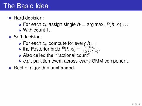
The Basic Idea

Hard decision:For each xi , assign single hi = arg maxh P(h, xi) . . .With count 1.

Soft decision:For each xi , compute for every h . . .the Posterior prob P̃(h|xi) = P(h,xi )P

h P(h,xi ).

Also called the “fractional count”e.g., partition event across every GMM component.

Rest of algorithm unchanged.

61 / 113

The Basic Idea

Initialize parameter values somehow.For each iteration . . .Expectation step: compute posterior (count) of h for each xi .

P̃(h|xi) =P(h, xi)Ph P(h, xi)

Maximization step: update parameters.Instead of data xi with hidden h, pretend . . .Non-hidden data where . . .(Fractional) count of each (h, xi) is P̃(h|xi).

62 / 113

Example: Training a 2-component GMM

Two-component univariate GMM; 10 data points.The data: x1, . . . , x10

8.4, 7.6, 4.2, 2.6, 5.1, 4.0, 7.8, 3.0, 4.8, 5.8

Initial parameter values:

p1 µ1 �21 p2 µ2 �2

20.5 4 1 0.5 7 1

Training data; densities of initial Gaussians.

63 / 113

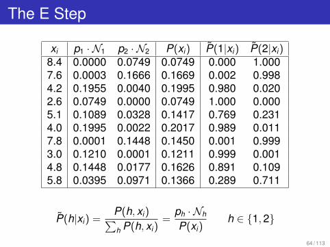
The E Step

xi p1 · N1 p2 · N2 P(xi) P̃(1|xi) P̃(2|xi)8.4 0.0000 0.0749 0.0749 0.000 1.0007.6 0.0003 0.1666 0.1669 0.002 0.9984.2 0.1955 0.0040 0.1995 0.980 0.0202.6 0.0749 0.0000 0.0749 1.000 0.0005.1 0.1089 0.0328 0.1417 0.769 0.2314.0 0.1995 0.0022 0.2017 0.989 0.0117.8 0.0001 0.1448 0.1450 0.001 0.9993.0 0.1210 0.0001 0.1211 0.999 0.0014.8 0.1448 0.0177 0.1626 0.891 0.1095.8 0.0395 0.0971 0.1366 0.289 0.711

P̃(h|xi) =P(h, xi)Ph P(h, xi)

=ph · Nh

P(xi)h 2 {1, 2}

64 / 113

The M Step

View: have non-hidden corpus for each component GMM.For hth component, have P̃(h|xi) counts for event xi .

Estimating µ: fractional events.

µ =1N

NX

i=1

xi ) µh =1

Pi P̃(h|xi)

NX

i=1

P̃(h|xi)xi

µ1 =1

0.000 + 0.002 + 0.980 + · · ·⇥

(0.000⇥ 8.4 + 0.002⇥ 7.6 + 0.980⇥ 4.2 + · · · )

= 3.98

Similarly, can estimate �2h with fractional events.

65 / 113

The M Step (cont’d)

What about the mixture weights ph?

To find MLE, count and normalize!

p1 =0.000 + 0.002 + 0.980 + · · ·

10= 0.59

66 / 113

The End Result

iter p1 µ1 �21 p2 µ2 �2

20 0.50 4.00 1.00 0.50 7.00 1.001 0.59 3.98 0.92 0.41 7.29 1.292 0.62 4.03 0.97 0.38 7.41 1.123 0.64 4.08 1.00 0.36 7.54 0.8810 0.70 4.22 1.13 0.30 7.93 0.12

67 / 113

First Few Iterations of EM

iter 0

iter 1

iter 2

68 / 113

Later Iterations of EM

iter 2

iter 3

iter 10

69 / 113

Why the EM Algorithm Works [3]

x = (x1, x2, . . .) = whole training set; h = hidden.✓ = parameters of model.Objective function for MLE: (log) likelihood.

L(✓) = log P(x|✓) = logX

h

P(h, x|✓)

Alternate objective functionWill show maximizing this equivalent to above

F (P̃, ✓) = L(✓)� D(P̃ k P✓)

P✓(h|x) = posterior over hidden.P̃(h) = distribution over hidden to be optimized . . .D(· k ·) = Kullback-Leibler divergence.

70 / 113

Why the EM Algorithm Works

F (P̃, ✓) = L(✓)� D(P̃ k P✓)

Outline of proof:Show that both E step and M step improve F (P̃, ✓).Will follow that likelihood L(✓) improves as well.

71 / 113

The E Step

F (P̃, ✓) = L(✓)� D(P̃ k P✓)

Properties of KL divergence.Nonnegative; and zero iff P̃ = P✓.

What is best choice for P̃(h)?Compute the current posterior P✓(h|x).Set P̃(h) equal to this posterior.

Since L(✓) is not function of P̃ . . .F (P̃, ✓) can only improve in E step.

72 / 113

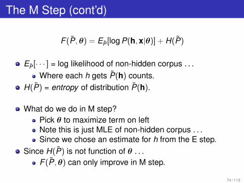
The M Step (cont’d)

F (P̃, ✓) = EP̃ [log P(h, x|✓)] + H(P̃)

EP̃ [· · · ] = log likelihood of non-hidden corpus . . .Where each h gets P̃(h) counts.

H(P̃) = entropy of distribution P̃(h).

What do we do in M step?Pick ✓ to maximize term on leftNote this is just MLE of non-hidden corpus . . .Since we chose an estimate for h from the E step.

Since H(P̃) is not function of ✓ . . .F (P̃, ✓) can only improve in M step.

74 / 113

Why the EM Algorithm Works

Observation: F (P̃, ✓) = L(✓) after E step (set P̃ = P✓).

F (P̃, ✓) = L(✓)� D(P̃ k P✓)

If F (P̃, ✓) improves with each iteration . . .And F (P̃, ✓) = L(✓) after each E step . . .L(✓) improves after each iteration.

There you go!

75 / 113

Discussion

EM algorithm is elegant and general way to . . .Train parameters in hidden models . . .To optimize likelihood.

Only finds local optimum.Seeding is of paramount importance.

Generalized EM algorithm.F (P̃, ✓) just needs to improve some in each step.i.e., P̃(h) in E step need not be exact posterior.i.e., ✓ in M step need not be ML estimate.e.g., can optimize Viterbi likelihood.

76 / 113

Where Are We?

1 The Expectation-Maximization Algorithm

2 Applying the EM Algorithm to GMM’s

77 / 113

Another Example Data Set

78 / 113

Question: How Many Gaussians?

Method 1 (most common): Guess!Method 2: Bayesian Information Criterion (BIC)[1].

Penalize likelihood by number of parameters.

BIC(Ck) =kX

j=1

{�12

nj log |⌃j |}� Nk(d +12

d(d + 1))

k = Gaussian components.d = dimension of feature vector.nj = data points for Gaussian j ; N = total data points.

79 / 113

The Bayesian Information Criterion

View GMM as way of coding data for transmission.Cost of transmitting model , number of params.Cost of transmitting data , log likelihood of data.

Choose number of Gaussians to minimize cost.

80 / 113

Question: How To Initialize Parameters?

Set mixture weights pj to 1/k (for k Gaussians).Pick N data points at random and . . .

Use them to seed initial values of µj .Set all �’s to arbitrary value . . .

Or to global variance of data.Extension: generate multiple starting points.

Pick one with highest likelihood.

81 / 113

Another Way: Splitting

Start with single Gaussian, MLE.Repeat until hit desired number of Gaussians:

Double number of Gaussians by perturbing means . . .Of existing Gaussians by ±✏.Run several iterations of EM.

82 / 113

Question: How Long To Train?

i.e., how many iterations of EM?Guess.Look at performance on training data.

Stop when change in log likelihood per event . . .Is below fixed threshold.

Look at performance on held-out data.Stop when performance no longer improves.

83 / 113

The Data Set

84 / 113

Sample From Best 1-Component GMM

85 / 113

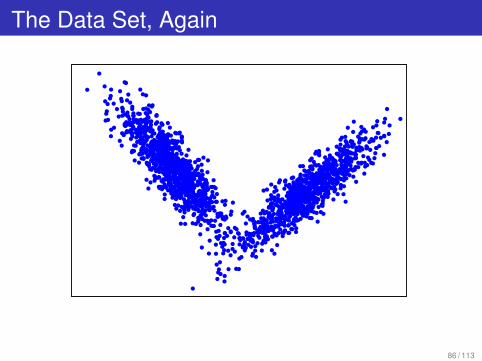
The Data Set, Again

86 / 113

20-Component GMM Trained on Data

87 / 113

20-Component GMM µ’s, �’s

88 / 113

Acoustic Feature Data Set

89 / 113

5-Component GMM; Starting Point A

90 / 113

5-Component GMM; Starting Point B

91 / 113

5-Component GMM; Starting Point C

92 / 113

Solutions With Infinite Likelihood

Consider log likelihood; two-component 1d Gaussian.

NX

i=1

ln

p1

1p2⇡�1

e� (xi�µ1)2

2�21 + p2

1p2⇡�2

e� (xi�µ2)2

2�22

!

If µ1 = x1, above reduces to

ln

1

2p

2⇡�1+

12p

2⇡�2e

12

(x1�µ2)2

�22

!+

NX

i=2

. . .

which goes to 1 as �1 ! 0.Only consider finite local maxima of likelihood function.

Variance flooring.Throw away Gaussians with “count” below threshold.

93 / 113

Recap

GMM’s are effective for modeling arbitrary distributions.State-of-the-art in ASR for decades.

The EM algorithm is primary tool for training GMM’s.Very sensitive to starting point.Initializing GMM’s is an art.

94 / 113

References

S. Chen and P.S. Gopalakrishnan, “Clustering via theBayesian Information Criterion with Applications in SpeechRecognition”, ICASSP, vol. 2, pp. 645–648, 1998.

A.P. Dempster, N.M. Laird, D.B. Rubin, “Maximum Likelihoodfrom Incomplete Data via the EM Algorithm”, Journal of theRoyal Stat. Society. Series B, vol. 39, no. 1, 1977.

R. Neal, G. Hinton, “A view of the EM algorithm that justifiesincremental, sparse, and other variants”, Learning inGraphical Models, MIT Press, pp. 355–368, 1999.

95 / 113

Where Are We: The Big Picture

Given test sample, find nearest training sample.


distance(A0test, A0

w)

Total distance between training and test sample . . .Is sum of distances between aligned frames.

distance⌧x ,⌧y (X , Y ) =TX

t=1


Goal: move from ad hoc distances to probabilities.

96 / 113

Gaussian Mixture Models

Assume many training templates for each word.Calc distance between set of training frames . . .And test frame.

framedist((x1, x2, . . . , xD); y)

Idea: use x1, x2, . . . , xD to train GMM: P(x).

framedist((x1, x2, . . . , xD); y)) � log P(y) !

97 / 113

What’s Next: Hidden Markov Models

Replace DTW with probabilistic counterpart.Together, GMM’s and HMM’s comprise . . .

Unified probabilistic framework.Old paradigm:


distance(A0test, A0

w)

New paradigm:

w⇤ = arg maxw2vocab

P(A0test|w)

98 / 113

lecture 4 gaussian mixture models...

Documents