lecture 4 reaction system as ordinary differential equations reaction system as stochastic process...
TRANSCRIPT

Lecture 4
•Reaction system as ordinary differential equations•Reaction system as stochastic process•Metabolic network and stoichiometric matrix•Graph spectral analysis/Graph spectral clustering and its application to metabolic networks

Introduction
Metabolism is the process through which living cells acquire energy and building material for cell components and replenishing enzymes.
Metabolism is the general term for two kinds of reactions: (1) catabolic reactions –break down of complex compounds to get energy and building blocks, (2) anabolic reactions—construction of complex compounds used in cellular functioning
How can we model metabolic reactions?

What is a Model?Formal representation of a system using--Mathematics--Computer program
Describes mechanisms underlying outputs
Dynamical models show rate of changes with time or other variable
Provides explanations and predictions
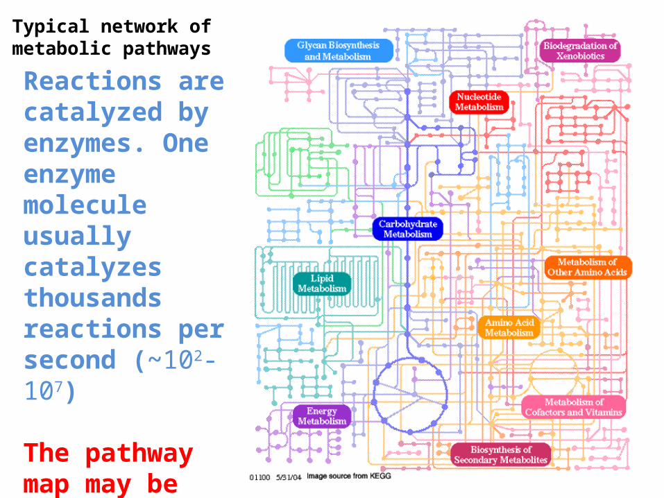
Typical network of metabolic pathways
Reactions are catalyzed by enzymes. One enzyme molecule usually catalyzes thousands reactions per second (~102-107)
The pathway map may be considered as a static model of metabolism

Dynamic modeling of metabolic reactions is the process of understanding the reaction rates i.e. how the concentrations of metabolites change with respect to time
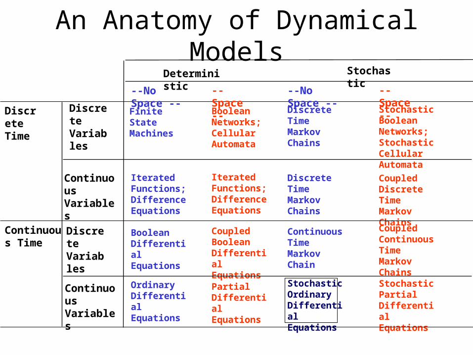
An Anatomy of Dynamical Models
DiscreteTime
DiscreteVariables
ContinuousVariables
Deterministic
--No Space -- -- Space --
Stochastic
--No Space -- -- Space --
Finite StateMachines
Boolean Networks;Cellular Automata
Discrete Time Markov Chains
Stochastic Boolean Networks;Stochastic Cellular Automata
Iterated Functions;Difference Equations
Iterated Functions;Difference Equations
Discrete Time Markov Chains
Coupled Discrete Time Markov Chains
Continuous Time
DiscreteVariables
ContinuousVariables
Boolean Differential Equations
Ordinary Differential Equations
Coupled Boolean Differential Equations
Partial Differential Equations
Continuous Time Markov Chain
Stochastic Ordinary Differential Equations
Coupled Continuous Time Markov Chains
Stochastic Partial Differential Equations

Differential equations
Differential equations are based on the rate of change of one or more variables with respect to one or more other variables

An example of a differential equation
Source: Systems biology in practice by E. klipp et al

An example of a differential equation
Source: Systems biology in practice by E. klipp et al

Source: Systems biology in practice by E. klipp et al
An example of a differential equation

Schematic representation of the upper part of the Glycolysis
Source: Systems biology in practice by E. klipp et al.

The ODEs representing this reaction system
Realize that the concentration of metabolites and reaction rates v1, v2, …… are functions of time
ODEs representing a reaction system

The rate equations can be solved as follows using a number of constant parameters

The temporal evaluation of the concentrations using the following parameter values and initial concentrations
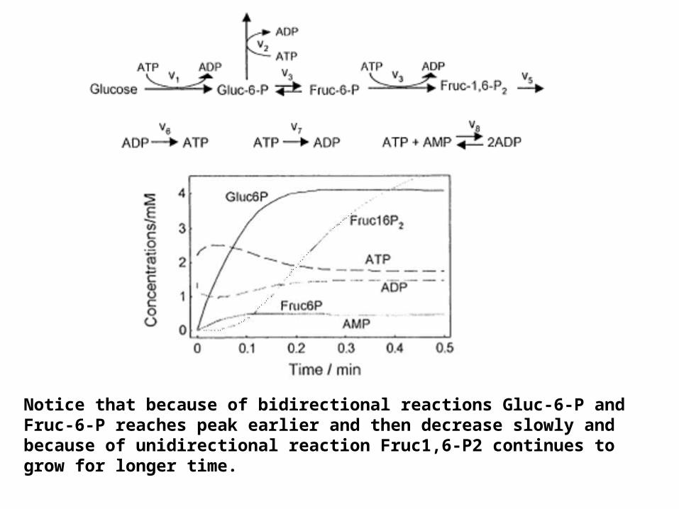
Notice that because of bidirectional reactions Gluc-6-P and Fruc-6-P reaches peak earlier and then decrease slowly and because of unidirectional reaction Fruc1,6-P2 continues to grow for longer time.

The use of differential equations assumes that the concentration of metabolites can attain continuous value.But the underlying biological objects , the molecules are discrete in nature.When the number of molecules is too high the above assumption is valid.But if the number of molecules are of the order of a few dozens or hundreds then discreteness should be considered.Again random fluctuations are not part of differential equations but it may happen for a system of few molecules.The solution to both these limitations is to use a stochastic simulation approach.
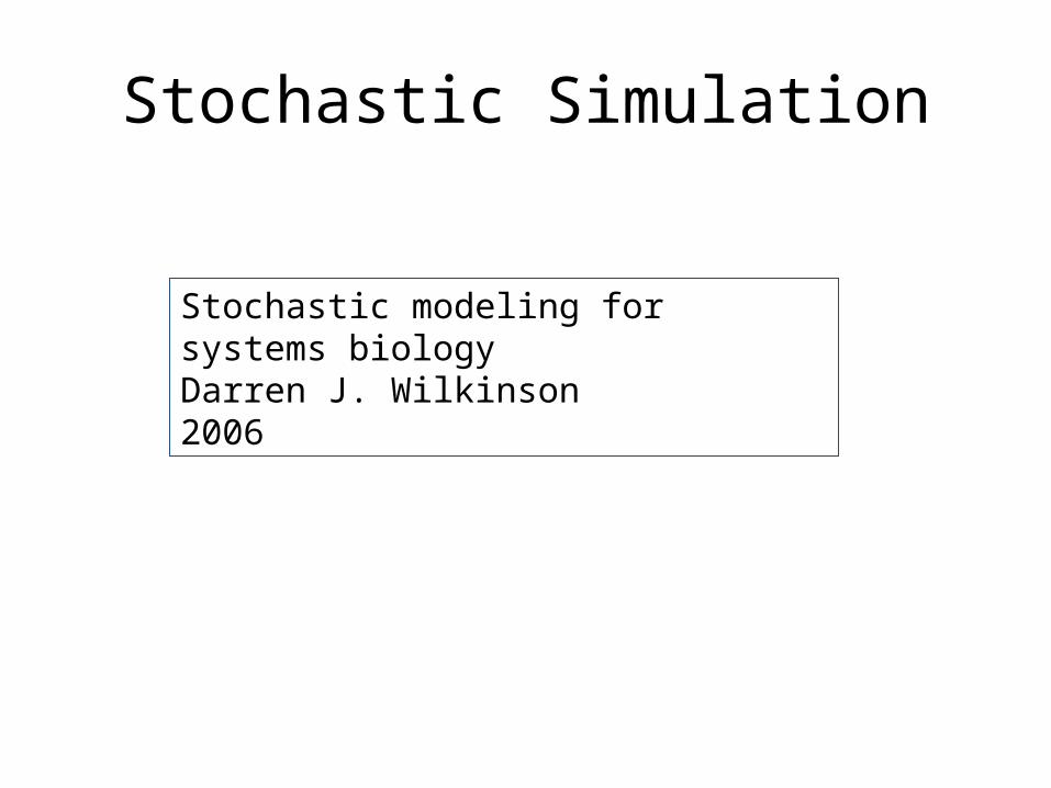
Stochastic Simulation
Stochastic modeling for systems biologyDarren J. Wilkinson2006

Molecular systems in cell

Molecular systems in cell[ ]: concentration of ith object
[m1(in)] [m2] [m3]
[m4]
[m5]
[m1(out)]
[r1] [r2] [r3] [r 4 ]
[p1][p2]
[p3]
[p4]

Molecular systems in cellcj: cj’: efficiency of jth process
[m1(in)] [m2] [m3]
[m4]
[m5]
[m1(out)]
[r1] [r2] [r3] [r 4 ]
[p1][p2]
[p3]
[p4]
c1
c2
c3 c4
c5c6
c7
c8
c9
c10
c11
c12
c13

Molecular systems for small molecules in cell
[m1(in)] [m2] [m3]
[m4]
[m5]
[m1(out)]
c1
c2
c3 c4
c5h1=c1 [m1(out)] h2=c2 [m1(in)]
h4=c5 [m2]
h3=c3 [m2] h5=c4 [m3]
c2 p1 ,r1
c5 p3 ,r3
c3 p2 ,r2 c4 p4 ,r4
Stochastic selection of reaction based on(h1, h2, h3, h4, h5)

Molecular systems for small molecules in cell
[m1(in)] [m2] [m3]
[m4]
[m5]
[m1(out)]=100
c1
c2
c3 c4
c5h1=c1 [m1(out)] = 100 c1
h2=c2 [m1(in)]
h4=c5 [m2]
h3=c3 [m2] h5=c4 [m3]
c2 p1 ,r1
c5 p3 ,r3
c5 p2 ,r2 c4 p4 ,r4
Stochastic selection of reaction based on(100 c1, h2, h3, h4, h5)Reaction 1

Molecular systems for small molecules in cell
[m1(in)]=1[m2]=0
[m3]=0
[m4]=0
[m5]=0
[m1(out)]=99
c1
c2
c3 c4
c5h1=c1 [m1(out)]= 99 c1
h2=c2 [m1(in)]= 1 c2
h4=c5 [m2]=0
h3=c3 [m2]=0
h5=c4 [m3]=0
Stochastic selection of Reaction based on (99 c1, 1 c2, 0, 0, 0) Reaction 1

Molecular systems for small molecules in cell
[m1(in)]=2[m2]=0
[m3]=0
[m4]=0
[m5]=0
[m1(out)]=98
c1
c2
c3 c4
c5h1=c1 [m1(out)]= 98 c1
h2=c2 [m1(in)]= 2 c2
h4=c5 [m2]=0
h3=c3 [m2]=0
h5=c4 [m3]=0
Stochastic selection of Reaction based on (98 c1, 2 c2, 0, 0, 0) Reaction 1

Molecular systems for small molecules in cell
[m1(in)]=3[m2]=0
[m3]=0
[m4]=0
[m5]=0
[m1(out)]=97
c1
c2
c3 c4
c5h1=c1 [m1(out)]= 97 c1
h2=c2 [m1(in)]= 3 c2
h4=c5 [m2]=0
h3=c3 [m2]=0
h5=c4 [m3]=0
Stochastic selection of Reaction based on (97 c1, 3 c2, 0, 0, 0) Reaction 2

Molecular systems for small molecules in cell
[m1(in)]=2[m2]=1
[m3]=0
[m4]=0
[m5]=0
[m1(out)]=97
c1
c2
c3 c4
c5h2=c2 [m1(in)]= 2 c2
h4=c5 [m2]=1 c5
h3=c3 [m2]=1 c3
h5=c4 [m3]=0
h1=c1 [m1(out)]= 97 c1
Stochastic selection of Reaction based on (97 c1, c2, 1 c3, 0, 1 c5) Reaction 1

Molecular systems for small molecules in cell
[m1(in)]=3 [m2]=1[m3]=0
[m4]=0
[m5]=0
[m1(out)]=96
c1
c2
c3 c4
c5h1=c1 [m1(out)]= 97 c1
h2=c2 [m1(in)]= 3 c2
h4=c5 [m2]=1 c5
h3=c3 [m2]=1 c3
h5=c4 [m3]=0
Stochastic selection of Reaction(96 c1, 3 c2, 1 c3, 0, 1 c5)Reaction 3

Molecular systems for small molecules in cell
[m1(in)]=3 [m2]=0[m3]=1
[m4]=0
[m5]=0
[m1(out)]=96
c1
c2
c3 c4
c5h1=c1 [m1(out)]= 97 c1
h2=c2 [m1(in)]= 3 c2
h4=c5 [m2]=0
h3=c3 [m2]=0
h5=c4 [m3]=1 c4
Stochastic selection of Reaction based on (96 c1, 3 c2, 0, 1 c4 , 0)…

Input data
[m1(in)] [m2] [m3]
[m4]
[m5]
[m1(out)]
c1
c2
c3 c4
c5
c1m1(out) m1(in)
c2m1(in) m2
c3m2 m3 m3 m5
c4
m2 m5
c5
[m1(out)] [m1(in)] [m2] [m3] [m4] [m5]Initial concentrations
Reaction parameters and Reactions

Gillespie AlgorithmStep 0: System Definitionobjects (i = 1, 2,…, n) and their initial quantities: Xi(init) reaction equations (j=1,2,…,m)
Rj: m(Pre)j1 X1 + ...+ m(Pre)
jn Xn = m (Post) j1 X1 +...+ m (Post)
jnXn
reaction intensities: ci for Rj
Step 4: Quantities for individual objects are revised base on selected reaction equation[Xi] ← [Xi] – m (Pre)
s + m(Post)s
Step 1: [Xi]Xi(init)
Step 2: hj: :probability of occurrence of reactions based on cj (j=1,2,..,m) and [Xi] (i=1,2,..,n)
Step 3: Random selection of reaction Here a selected reaction is represented by index s.

Gillespie Algorithm (minor revision)
Step 0: System Definitionobjects (i = 1, 2,…, n) and their initial quantities Xi(init) reaction equations (j=1,2,…,m)Rj: m(Pre)
j1 X1 + ...+ m(Pre)jn Xn = m (Post)
j1 X1 +...+ m (Post) jnXn
reaction intensities: ci for Rj
Step 4: Quantities for individual objects are revised base on selected reaction equation X’i = [Xi] – m (Pre)
s + m(Post)s
Step 1: [Xi]Xi(init)
Step 2: hj: :probability of occurrence of reactions based on cj (j=1,2,..,m) and [Xi] (i=1,2,..,n)
Step 3: Random selection of reaction Here a selected reaction is represented by index s.
X’i 0No
Step 5: [Xj] X’i
YesX’i Xi
max No
Yes
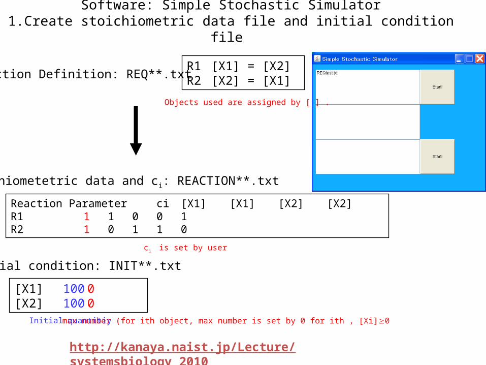
Software: Simple Stochastic Simulator1.Create stoichiometric data file and initial condition file
Reaction Definition: REQ**.txtR1 [X1] = [X2]R2 [X2] = [X1]
Reaction Parameter ci [X1] [X1] [X2] [X2]R1 1 1 0 0 1R2 1 0 1 1 0
Stoichiometetric data and ci: REACTION**.txt
ci is set by user
[X1] 100 0[X2] 100 0
Initial condition: INIT**.txt
max number (for ith object, max number is set by 0 for ith , [Xi]0 Initial quantitiy
Objects used are assigned by [ ] .
http://kanaya.naist.jp/Lecture/systemsbiology_2010

Software: Simple Stochastic Simulator2. Stochastic simulation
Stoichiometetric data and ci: REACTION**.txt
Initial condition: INIT**.txt
Reaction Parameterc: 1.0 1.0//time [X1] [X2]0.00 100.0 100.00.0015706073545097992 101.0 99.00.015704610011372147 100.0 100.00.01670413203960951 101.0 99.0….….
Simulation results: SIM**.txt
0
50
100
150
0 10 20 30 40 50
[X1]
[X2]

Example of simulation results# of type of chemicals =2

0
100
200
300
400
500
600
700
800
900
1000
0 2 4 6 8
[X1][X2]
[X1][X2] c=1, [X1]=1000, [X2]=0

[X1][X2] [X2][X1]c1=c2=1[X1]=1000
0
100
200
300
400
500
600
700
800
900
1000
0 1 2 3 4 5 6 7 8 9 10
[X1][X2]

# of type of chemicals =3
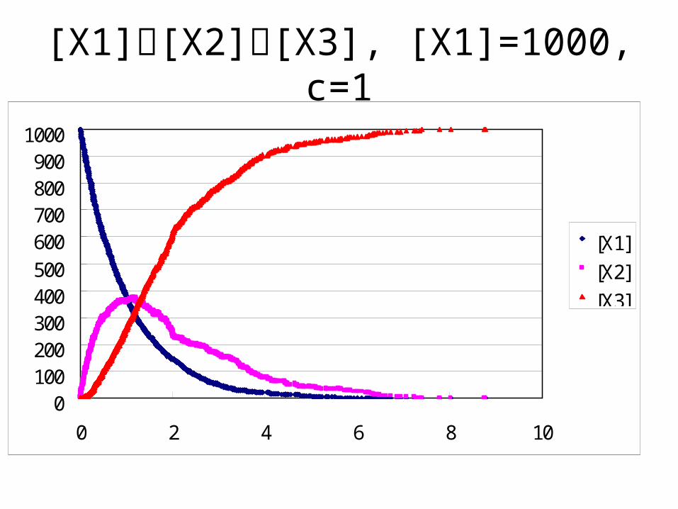
[X1][X2][X3], [X1]=1000, c=1
01002003004005006007008009001000
0 2 4 6 8 10
[X1][X2][X3]

[X1] [X2][X3], [X1]=1000, c=1
0
100
200
300
400
500
600
700
800
900
1000
0 5 10 15 20
[X1][X2][X3]

[X1][X2][X3], [X1]=1000, c=1
0
100
200
300
400
500
600
700
800
900
1000
0 2 4 6 8 10
[X1][X2][X3]

[X1][X2][X3],[X1]=1000, c=1
0
100
200
300
400
500
600
700
800
900
1000
0 2 4 6 8
[X1][X2][X3]

loop reaction [X1][X2][X3][X1], [X1]=1000, c=1
0
100
200
300
400
500
600
700
800
900
1000
0 2 4 6 8 10
[X1][X2][X3]

Representation of ReactionData Set
[X1] 2[X1]c1
[X1] + [X2] 2[X2]c2
[X2] Φc3
Reaction Data Initial Condition
[X1]= X1(init)
[X2]= X2(init)

Example 2 EMP
glcK ATP + [D-glucose] -> ADP + [D-glucose-6-phosphate]glcK ATP + [alpha-D-glucose] -> ADP + [D-glucose-6-phosphate]pgi [D-glucose-6-phosphate] <-> [D-fructose-6-phosphate]pgi [D-fructose-6-phosphate] <-> [D-glucose-6-phosphate]pgi [alpha-D-glucose-6-phosphate] <-> [D-fructose-6-phosphate]pgi [D-fructose-6-phosphate] <-> [alpha-D-glucose-6-phosphate] pfk ATP + [D-fructose-6-phosphate] -> ADP + [D-fructose-1,6-bisphosphate]fbp [D-fructose-1,6-bisphosphate] + H(2)O -> [D-fructose-6-phosphate] + phosphatefbaA [D-fructose-1,6-bisphosphate] <-> [glycerone-phosphate] + [D-glyceraldehyde-3-phosphate]fbaA [glycerone-phosphate] + [D-glyceraldehyde-3-phosphate] <-> [D-fructose-1,6-bisphosphate]tpiA [glycerone-phosphate] <-> [D-glyceraldehyde-3-phosphate]tpiA [D-glyceraldehyde-3-phosphate] <-> [glycerone-phosphate]gapA [D-glyceraldehyde-3-phosphate] + phosphate + NAD(+) -> [1,3-biphosphoglycerate] + NADH + H(+)gapB [1,3-biphosphoglycerate] + NADPH + H(+) -> [D-glyceraldehyde-3-phosphate] + NADP(+) + phosphatepgk ADP + [1,3-biphosphoglycerate] <-> ATP + [3-phospho-D-glycerate]pgk ATP + [3-phospho-D-glycerate] <-> ADP + [1,3-biphosphoglycerate]pgm [3-phospho-D-glycerate] <-> [2-phospho-D-glycerate]pgm [2-phospho-D-glycerate] <-> [3-phospho-D-glycerate]eno [2-phospho-D-glycerate] <-> [phosphoenolpyruvate] + H(2)Oeno [phosphoenolpyruvate] + H(2)O <-> [2-phospho-D-glycerate]

Example 2 EMP
D-glucose alpha-D-glucose
D-fructose-6-phosphatealpha-D-glucose-6-phosphate
[D-fructose-1,6-bisphosphate]
[D-glyceraldehyde-3-phosphate]
D-glucose-6-phosphate
[glycerone-phosphate]
[1,3-biphosphoglycerate]
[3-phospho-D-glycerate]
[2-phospho-D-glycerate]
[phosphoenolpyruvate]

Metabolic network and stoichiometric matrix

Typical network of metabolic pathways
Reactions are catalyzed by enzymes. One enzyme molecule usually catalyzes thousands reactions per second (~102-107)
The pathway map may be considered as a static model of metabolism

For a metabolic network consisting of m substances and r reactions the system dynamics is described by systems equations.
The stoichiometric coefficients nij assigned to the substance Si and the reaction vj can be combined into the so called stoichiometric matrix.
What is a stoichiometric matrix?

Example reaction system and corresponding stoichiometric matrix
There are 6 metabolites and 8 reactions in this example system
stoichiometric matrix
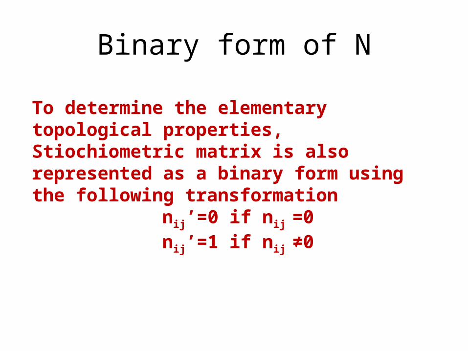
Binary form of N
To determine the elementary topological properties, Stiochiometric matrix is also represented as a binary form using the following transformation
nij’=0 if nij =0nij’=1 if nij ≠0

Stiochiometric matrix is a sparse matrix
Source: Systems biology by Bernhard O. Palsson

Information contained in the stiochiometric matrix
Stiochiometric matrix contains many information e.g. about the structure of metabolic network , possible set of steady state fluxes, unbranched reaction pathways etc. 2 simple information:•The number of non-zero entries in column i gives the number of compounds that participate in reaction i.
•The number of non-zero entries in row j gives the number of reactions in which metabolite j participates.
So from the stoicheometric matrix, connectivities of all the metabolites can be computed

Information contained in the stiochiometric matrix
There are relatively few metabolites (24 or so) that are highly connected while most of the metabolites participates in only a few reactions
Source: Systems biology by Bernhard O. Palsson

Information contained in the stiochiometric matrix
In steady state we know that
The right equality sign denotes a linear equation system for determining the rates v
This equation has non trivial solution only for Rank N < r(the number of reactions)
K is called kernel matrix if it satisfies NK=0
The kernel matrix K is not unique

The kernel matrix K of the stoichiometric matrix N that satisfies NK=0, contains (r- Rank N) basis vectors as columns
Every possible set of steady state fluxes can be expressed as a linear combination of the columns of K
Information contained in the stiochiometric matrix

-
With α1= 1 and α2 = 1, , i.e. at steady state v1 =2, v2 =-1 and v3 =-1
Information contained in the stiochiometric matrix
And for steady state flux it holds that J = α1 .k1 + α2.k2
That is v2 and v3 must be in opposite direction of v1 for the steady state corresponding to this kernel matrix which can be easily realized.
Information contained in the stiochiometric matrix
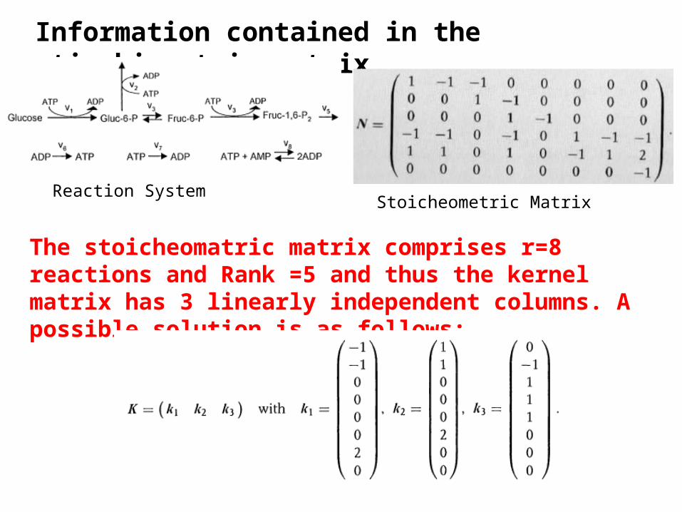
Reaction SystemStoicheometric Matrix
The stoicheomatric matrix comprises r=8 reactions and Rank =5 and thus the kernel matrix has 3 linearly independent columns. A possible solution is as follows:

Information contained in the stiochiometric matrix
Reaction System
The entries in the last row of the kernel matrix is always zero. Hence in steady state the rate of reaction v8 must vanish.

Reaction System
The entries for v3 , v4 and v5 are equal for each column of the kernel matrix, therefore reaction v3 , v4 and v5 constitute an unbranched pathway . In steady state they must have equal rates
Information contained in the stiochiometric matrix
If all basis vectors contain the same entries for a set of rows, this indicate an unbranched reaction path

Elementary flux modes and extreme pathwaysThe definition of the term pathway in a metabolic network is not straightforward.
A descriptive definition of a pathway is a set of subsequent reactions that are in each case linked by common metabolites
Fluxmodes are possible direct routes from one external metabolite to another external metabolite.
A flux mode is an elementary flux mode if it uses a minimal set of reactions and cannot be further decomposed.

Elementary flux modes and extreme pathways

Elementary flux modes and extreme pathways
Extreme pathway is a concept similar to elementary flux modeThe extreme pathways are a subset of elementary flux modes
The difference between the two definitions is the representation of exchange fluxes. If the exchange fluxes are all irreversible the extreme pathways and elementary modes are equivalent
If the exchange fluxes are all reversible there are more elementary flux modes than extreme pathways
One study reported that in human blood cell there are 55 extreme pathways but 6180 elementary flux modes

Elementary flux modes and extreme pathways
Source: Systems biology by Bernhard O Palsson

Elementary flux modes and extreme pathways
Elementary flux modes and extreme pathways can be used to understand the range of metabolic pathways in a network, to test a set of enzymes for production of a desired product and to detect non redundant pathways, to reconstruct metabolism from annotated genome sequences and analyze the effect of enzyme deficiency, to reduce drug effects and to identify drug targets etc.

Lecture7Topic1: Graph spectral analysis/Graph spectral clustering and its application to metabolic networksTopic 2: Concept of Line GraphsTopic 3: Introduction to Cytoscape
Graph spectral analysis/
Graph spectral clustering

PROTEIN STRUCTURE: INSIGHTS FROM GRAPH THEORY
bySARASWATHI VISHVESHWARA, K. V. BRINDA and N. KANNANy
Molecular Biophysics Unit, Indian Institute of ScienceBangalore 560012, India

Laplacian matrix L=D-A
Adjacency Matrix Degree Matrix

Eigenvalues of a matrix A are the roots of the following equation
|A-λI|=0, where I is an identity matrix
Let λ is an eigenvalue of A and x is a vector such that
then x is an eigenvector of A corresponding to λ .
-----(1)N×N N×1 N×1
Eigenvalues and eigenvectors

Node 1 has 3 edges, nodes 2, 3 and 4 have 2 edges each and node 5 has only one edge. The magnitude of the vector components of the largest eigenvalue of the Adjacency matrix reflects this observation.

Node 1 has 3 edges, nodes 2, 3 and 4 have 2 edges each and node 5 has only one edge. Also the magnitude of the vector components of the largest eigenvalue of the Laplacian matrix reflects this observation.

The largest eigenvalue (lev) depends upon the highest degree in the graph. For any k regular graph G (a graph with k degree on all the vertices), the eigenvalue with the largest absolute value is k. A corollary to this theorem is that the lev of a clique of n verticesis n − 1. In a general connected graph, the lev is always less than or equal to (≤ ) to the largest degree in the graph. In a graph with n vertices, the absolute value of lev decreasesas the degree of vertices decreases. The lev of a clique with 11 vertices is 10 and that of a linearchain with 11 vertices is 1.932
a linear chain with 11 vertices
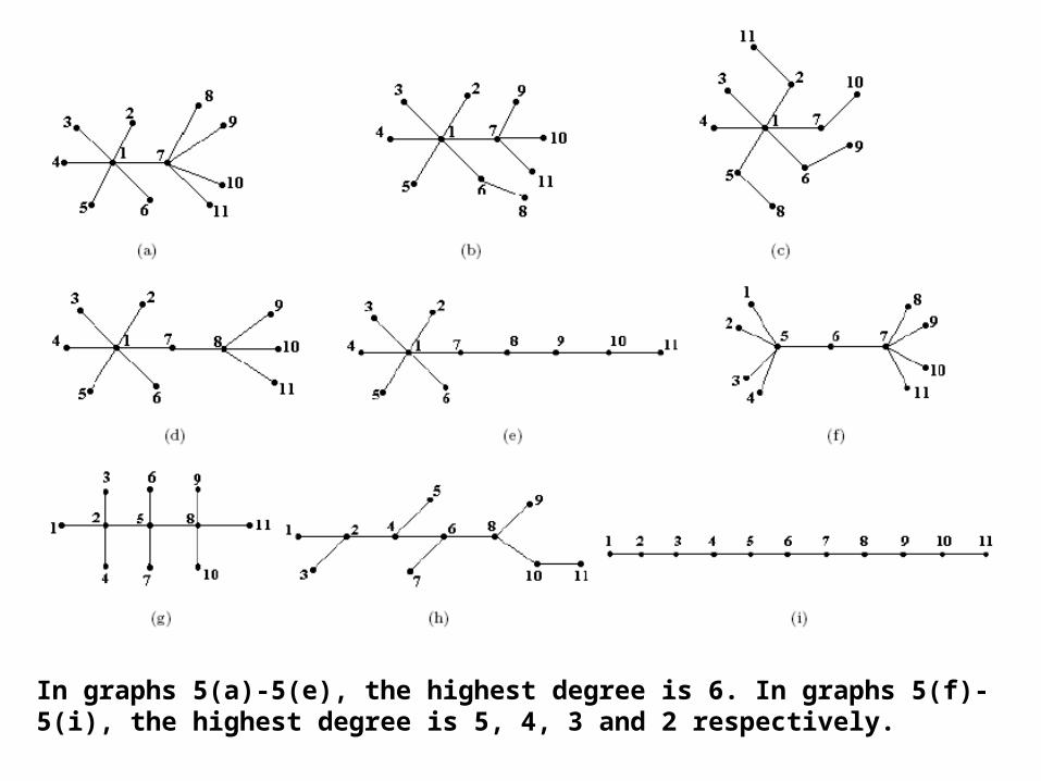
In graphs 5(a)-5(e), the highest degree is 6. In graphs 5(f)-5(i), the highest degree is 5, 4, 3 and 2 respectively.

It can be noticed that the lev is generally higher if the graph contains vertices of high degree. The lev decreases gradually from the graph with highest degree 6 to the one with highest degree 2. In case of graphs 5(a)-5(e), where there is one common vertex with degree 6 (highest degree) and the degrees of the other vertices are different (less than 6 in all cases), the lev differs i.e. the lev also depends on the degree of the vertices adjoining the highest degree vertex.

This paper combines graph 4(a) and graph 4(b) and constructs a Laplacian matrix with edge weights (1/dij ), where dij is the distance between vertices i and j. The distances between the vertices of graph 4(a) and graph 4(b) are considered to be very large (say 100) and thus the matrix elements corresponding to a vertex from graph 4(a) and the other from graph 4(b) is considered to have a very small value of 0.01. The Laplacian matrix of 8 vertices thus considered is diagonalized and their eigenvalues and corresponding vector components are given in Table 3.

The vector components corresponding to the second smallest eigenvalue contains the desired information about clustering, where the cluster forming residues have identical values. In Fig. 4, nodes 1-5 form a cluster (cluster 1) and 6-8 form another cluster (cluster 2).

Metabolome Based Reaction Graphs of M. tuberculosis and M. leprae: A Comparative Network Analysisby
Ketki D. Verkhedkar1, Karthik Raman2, Nagasuma R. Chandra2, Saraswathi Vishveshwara1*1 Molecular Biophysics Unit, Indian Institute of Science, Bangalore, India, 2 Bioinformatics Centre, Supercomputer Education and Research Centre, Indian Institute of Science, Bangalore, IndiaPLoS ONE | www.plosone.org September 2007 | Issue 9 | e881

Construction of network
R1 R2
R3 R4
Stoichrometric matrix
Following this method the networks of metabolic reactions corresponding to 3 organisms were constructed

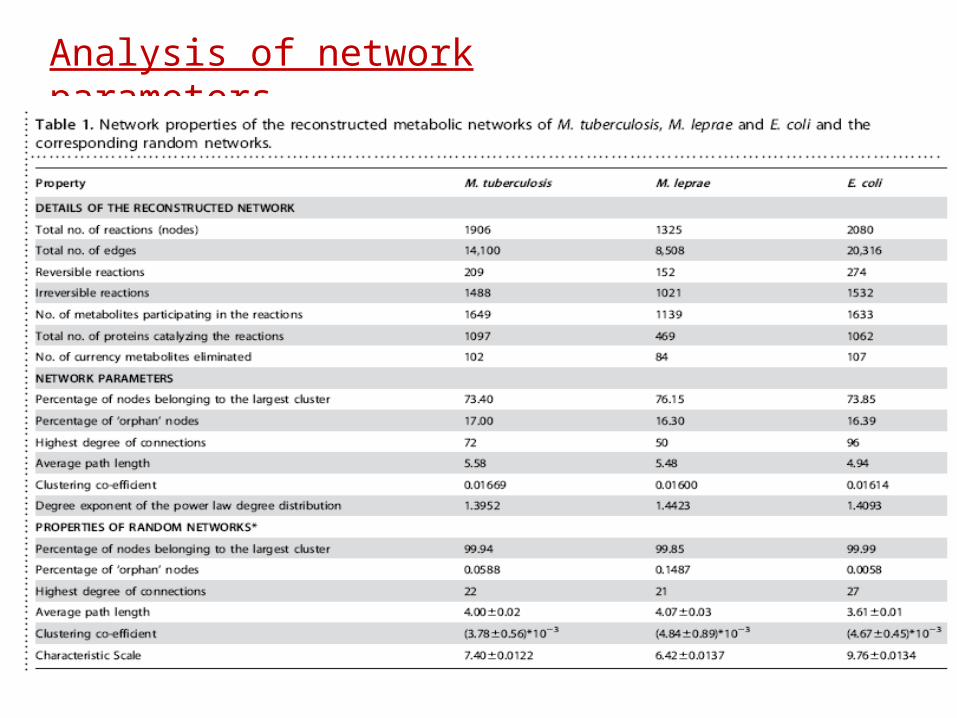
Analysis of network parameters

Giant component of the reaction network of e.coli

Giant components of the reaction networks of M. tuberculosis and M. leprae

Analyses of sub-clusters in the giant componentGraph spectral analysis was performed to detect sub-clusters of reactions in the giant component.To obtain the eigenvalue spectra of the graph, the adjacency matrix of the graph is converted to a Laplacian matrix (L), by the equation:L=D-Awhere D, the degree matrix of the graph, is a diagonal matrix in which the ith element on the diagonal is equal to the number of connections that the ith node makes in the graph.
It is observed that reactions belonging to fatty acid biosynthesis and the FAS-II cycle of the mycolic acid pathway in M. tuberculosis form distinct, tightly connected sub-clusters.


Identification of hubs in the reaction networksIn biological networks, the hubs are thought to be functionally important and phylogenetically oldest.
The largest vector component of the highest eigenvalue of the Laplacian matrix of the graph corresponds to the node with high degree as well as low eccentricity. Two parameters, degree and eccentricity, are involved in the identification of graph spectral (GS) hubs.

Identification of hubs in the reaction networks
Alternatively, hubs can be ranked based on their connectivity alone (degree hubs).
It was observed that the top 50 degree hubs in the reaction networks of the three organisms comprised reactions involving the metabolite L-glutamate as well as reactions involving pyruvate. However, the top 50 GS hubs of M. tuberculosis and M. leprae exclusively comprised reactions involving L-glutamate while the top GS hubs in E. coli only consisted of reactions involving pyruvate.
The difference in the degree and GS hubs suggests that the most highly connected reactions are not necessarily the most central reactions in the metabolome of the organism
