lecture 4a: arma model - miami university · • however, arma model cannot be applied to any time...
TRANSCRIPT

Lecture 4a: ARMA Model
1

Big Picture
• Most often our goal is to find a statistical model to describe real
time series (estimation), and then predict the future (forecasting)
• One particularly popular model is ARMA model
• Using ARMA model to describe real time series is called
Box-Jenkins Methodology
• However, ARMA model cannot be applied to any time series.
The ideal series should be stationary and ergodic!
2

(Weak or Covariance) Stationarity
A time series {yt} is (weakly or covariance) stationary if it satisfies
the following properties: ∀t
Eyt = µ (1)
var(yt) = σ2y (2)
cov(yt, yt−j) depends only on j (3)
So in words, a stationary series has constant (time-invariant) mean,
constant variance, and its (auto)covariance depends on the lag only.
A series is nonstationary if any of those is violated.
3

Why Stationarity?
• Stationarity is a nice property.
• Suppose we have two samples of data for the same time series.
One sample is from year 1981 to 1990; the other is from year
1991 to 2000. If the series is stationary, then the two samples
should give us approximately the same estimates for mean,
variance and covariance since those moments do not depend on t
under stationarity.
• If, on the other hand, the two samples produce significantly
different estimates, then the series is most likely to have
structural breaks and is nonstationary.
• Using history to forecast future cannot be justified unless
stationarity holds.
4

Example of Nonstationary Series
Consider a trending series given by
yt = at+ et
where et is white noise. This trending series is nonstationary because
the expectation value is
Eyt = at,
which changes with t, and is not constant
5

Ergodicity
• A time series is ergodic if, as the lag value increases, its
autocovariance decays to zero fast enough.
cov(yt, yt−j) → 0 fast enough as j → ∞
• For a series which is both stationary and ergodic, the law of large
number holds
1
T
T∑t=1
yt → E(yt), as T → ∞
• Later we will learn that a unit root process is not ergodic, so the
law of large number cannot be applied to a unit root process.
6
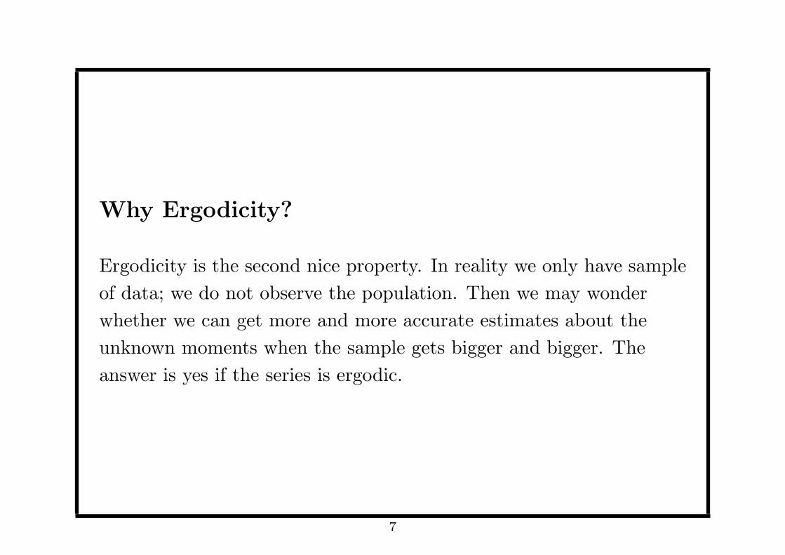
Why Ergodicity?
Ergodicity is the second nice property. In reality we only have sample
of data; we do not observe the population. Then we may wonder
whether we can get more and more accurate estimates about the
unknown moments when the sample gets bigger and bigger. The
answer is yes if the series is ergodic.
7

BoxJenkins Methodology
• We first derive the dynamic properties of a hypothetical ARMA
process
• We next find the dynamic pattern of a real time series
• Finally we match the real time series with the possibly closest
hypothetical ARMA process (model).
8

Review: Expectation and Variance
Let X,Y be two random variables, and a, b are constant numbers.
We have
E(aX + bY ) = aE(X) + bE(Y ) (4)
var(X) ≡ E[(X − EX)2] = E(X2)− (EX)2 (5)
var(aX) = a2var(X) (6)
cov(X,Y ) ≡ E[(X − EX)(Y − EY )] (7)
cov(X,X) = var(X) (8)
cov(X,Y ) = 0 ⇔ X,Y are uncorrelated (9)
var(aX + bY ) = a2var(X) + b2var(Y ) + 2abcov(X,Y ) (10)
9
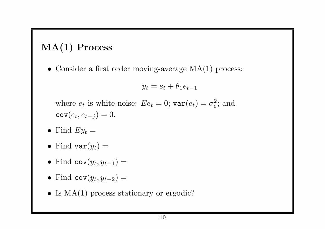
MA(1) Process
• Consider a first order moving-average MA(1) process:
yt = et + θ1et−1
where et is white noise: Eet = 0; var(et) = σ2e ; and
cov(et, et−j) = 0.
• Find Eyt =
• Find var(yt) =
• Find cov(yt, yt−1) =
• Find cov(yt, yt−2) =
• Is MA(1) process stationary or ergodic?
10
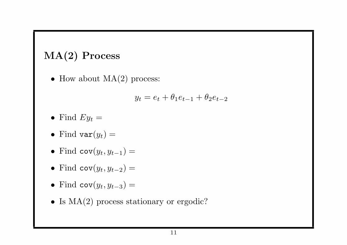
MA(2) Process
• How about MA(2) process:
yt = et + θ1et−1 + θ2et−2
• Find Eyt =
• Find var(yt) =
• Find cov(yt, yt−1) =
• Find cov(yt, yt−2) =
• Find cov(yt, yt−3) =
• Is MA(2) process stationary or ergodic?
11

In General: MA(q) Process
A general MA(q) process (with a constant) is
yt = θ0 + et + θ1et−1 + θ2et−2 + . . . θqet−q (11)
We can show a MA(q) process is stationary and ergodic because
Eyt = θ0
var(yt) = (1 + θ21 + . . .+ θq)2σ2
e
cov(yt, yt−j) =
f(j) = 0, if j = 1, 2, . . . , q
0, if j = q + 1, q + 2, . . .
So the MA process is characterized by the fact that its
autocovariance becomes zero (truncated) after q-th lag.
12

Impulse Response
• The MA process can also be characterized by its impulse
response (ie., the effect of past shocks on y).
• It follows directly from (11) that
dytdet−j
=
θj , if j = 1, 2, . . . , q
0, if j = q + 1, q + 2, . . .
• So the impulse response for MA(q) process is truncated after q-th
lag.
13

AR(1) Process
• A first order autoregressive or AR(1) process is synonymous with
the first order stochastic difference equation:
yt = ϕ0 + ϕ1yt−1 + et
where et is white noise.
• From lecture 3 we know this process is stationary if
|ϕ1| < 1
• If ϕ1 = 1, it becomes a unit-root process (called random walk),
which is nonstationary and non-ergodic.
14

Stationary AR(1) Process
Assuming |ϕ1| < 1 (so stationarity holds)
• Find Eyt =
• Find γ0 ≡ var(yt) =
• Find γ1 ≡ cov(yt, yt−1) =
• Find γ2 ≡ cov(yt, yt−2) =
• Find γj ≡ cov(yt, yt−j) =
15

Autocovariance and Ergodicity
• For a stationary AR(1) process, its autocovariance follows a first
order deterministic difference equation (called Yule Walker
equation)
γj = ϕ1γj−1
• The solution of the Yule Walker equation is
γj = ϕj1γ0, (j = 1, 2, . . .)
• A stationary AR(1) process with |ϕ1| < 1 is ergodic because
γj → 0 fast enough as j → ∞
In this case we have geometric decay for the autocovariance.
16

Autocorrelation Function (ACF)
• The j-th autocorrelation ρj is defined as
ρj ≡γjγ0
It is a function of j, and is unit-free.
• For a stationary AR(1) process we have
ρj = ϕj1
so the ACF decays to zero fast enough (like a geometric series) as
j rises (but never be truncated)
• This fact can be used as an identification tool for AR process.
17

MA(∞) Form
• AR(1) process can be equivalently written as an infinite-order
moving averaging process MA(∞)
• Repeatedly using the method of iteration we can show
yt = ϕ0 + ϕ1yt−1 + et
= ϕ0 + ϕ1(ϕ0 + ϕ1yt−2 + et−1) + et
= ϕ0 + ϕ1ϕ0 + ϕ21yt−2 + et + ϕ1et−1
= . . .+ ϕ21(ϕ0 + ϕ1yt−3 + et−2) + . . .
= . . .
18

MA(∞) Form
• In the end we have (assuming |ϕ1| < 1)
yt =ϕ0
1− ϕ1+ et + ϕ1et−1 + ϕ2
1et−2 + . . .
• Note that the j-th coefficient in the MA(∞) form looks special
θj = ϕj1
which decays to zero as j rises
• So the impulse response for a stationary AR(1) process decays to
zero in the limit (and never be truncated)
19

Lag Operator
• Define a lag operator L as
Lyt = yt−1, L2yt = L(Lyt) = Lyt−1 = yt−2, . . .
• In general
Ljyt = yt−j
In words applying the lag operator once amounts to pushing the
series one period back
• Loosely speaking, you can treat L as a number in the following
math derivation
20

MA(∞) Form Revisited
• We can derive the MA(∞) form easily using the lag operator
• The AR(1) process can be written as
yt = ϕ0 + ϕ1yt−1 + et (12)
⇒ yt = ϕ0 + ϕ1Lyt + et (13)
⇒ (1− ϕ1L)yt = ϕ0 + et (14)
⇒ yt =1
1− ϕ1L(ϕ0 + et) (15)
⇒ yt = (1 + ϕ1L+ ϕ21L
2 + . . .)(ϕ0 + et) (16)
⇒ yt =ϕ0
1− ϕ1+ et + ϕ1et−1 + ϕ2
1et−2 + . . . (17)
where the last equality follows because Lc = c when c is constant.
21

Lecture 4b: Estimate ARMA Model
22

BoxJenkins Methodology: Identification (I)
• For a real time series we first check whether it is stationary. A
trending series is not stationary.
• Suppose the real time series is stationary, then we can compute
the sample mean, sample variance and sample covariance as
µ =1
T
T∑t=1
yt (18)
γ0 =1
T − 1
T∑t=1
(yt − µ)2 (19)
γj =1
T − j − 1
T∑t=j+1
(yt − µ)(yt−j − µ) (20)
23

BoxJenkins Methodology: Identification (II)
• Next we compute the sample autocorrelation function (SACF)
ρj =γjγ0
(j = 1, 2, . . .)
• We compare the pattern of SACF to that of the AR, MA or
ARMA process. The closest match leads to the chosen model.
• For example, we model a real series using an AR(1) model if the
SACF has the pattern implied by the AR(1) model.
24

Estimate AR Model
• Fitting AR(p) model means running a p-th order autoregression:
yt = ϕ0 + ϕ1yt−1 + . . .+ ϕpyt−p + ut
• In this (auto)regression, dependent variable is yt, and the first p
lagged values are used as regressors.
• Note I denote the error term by ut, not et. That means the error
term may or may not be white noise.
• The error term is white noise only if this AR(p) regression is
adequate, or in other words, yt−p−1 and other previous values are
not needed in the regression.
25
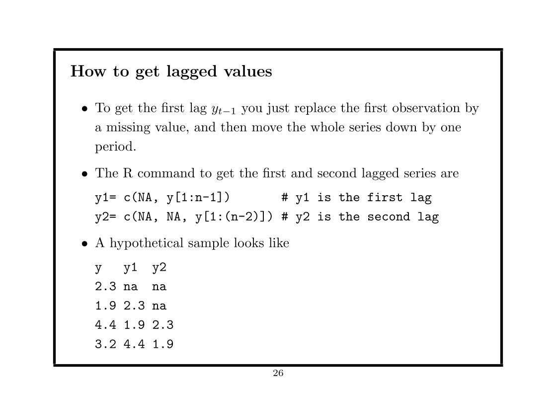
How to get lagged values
• To get the first lag yt−1 you just replace the first observation by
a missing value, and then move the whole series down by one
period.
• The R command to get the first and second lagged series are
y1= c(NA, y[1:n-1]) # y1 is the first lag
y2= c(NA, NA, y[1:(n-2)]) # y2 is the second lag
• A hypothetical sample looks like
y y1 y2
2.3 na na
1.9 2.3 na
4.4 1.9 2.3
3.2 4.4 1.9
26

OLS
• The AR(p) autoregression is estimated by ordinary least squares
(OLS).
• The only thing special here is that the regressors are the lagged
values of the dependent variable (other than other series).
27
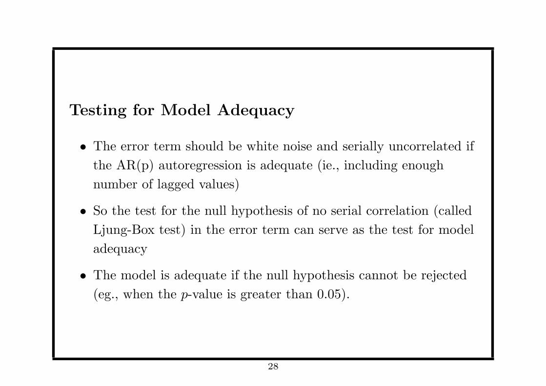
Testing for Model Adequacy
• The error term should be white noise and serially uncorrelated if
the AR(p) autoregression is adequate (ie., including enough
number of lagged values)
• So the test for the null hypothesis of no serial correlation (called
Ljung-Box test) in the error term can serve as the test for model
adequacy
• The model is adequate if the null hypothesis cannot be rejected
(eg., when the p-value is greater than 0.05).
28

R code
The R command for running an AR(2) regression and testing its
adequacy are
ar2 = lm(y~y1+y2)
summary(ar2)
Box.test (ar2$res, lag = 1, type="Ljung")
29

Overfitting
• It is possible that the AR(p) autoregression overfits the data (ie.,
including some unnecessary lagged values)
• The AR(p) autoregression overfits when some of the coefficients
are statistically insignificant (with p-value for the coefficient
greater than 0.05)
• Next we can drop those insignificant coefficients
30

Three Strategies
• (Principle of Parsimony): we start with AR(1), and keep adding
additional lagged values as new regressors until the error term
becomes white noise
• (General to Specific): we start with AR(p), and keep deleting
insignificant lagged values until all remaining ones are significant
• (Information Criterion): we try several AR models with different
lags, and pick the one with smallest AIC (Akaike information
criterion)
• The information criterion approach is most popular
31
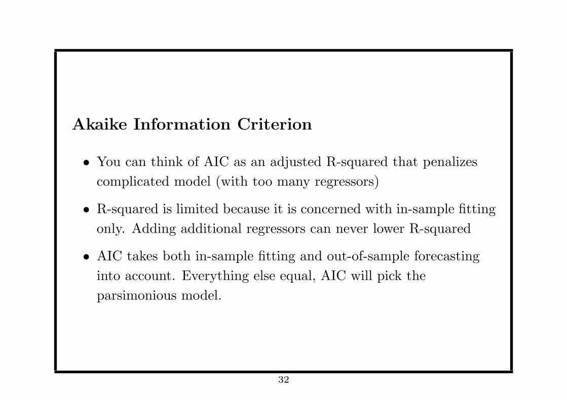
Akaike Information Criterion
• You can think of AIC as an adjusted R-squared that penalizes
complicated model (with too many regressors)
• R-squared is limited because it is concerned with in-sample fitting
only. Adding additional regressors can never lower R-squared
• AIC takes both in-sample fitting and out-of-sample forecasting
into account. Everything else equal, AIC will pick the
parsimonious model.
32

Interpreting Error Term (Optional)
• The error term ut becomes white noise et if the model is
adequate.
• For a white noise error term, it can also be interpreted as the
prediction error
et ≡ yt − E(yt|yt−1, yt−2, . . .)
where the conditional mean E(yt|yt−1, yt−2, . . .) is the best
predictor for yt given its history (yt−1, yt−2, . . .).
33

Estimate MA Model (Optional)
• MA model is much harder to estimate than AR model
• The advice for practitioners is that don’t use MA or ARMA
model unless AR model does very bad job.
34

Estimate MA(1) Model (Optional)
yt = et + θet−1
• We cannot run a regression here because et is unobservable.
• Instead, we need to apply the method of maximum likelihood
(ML).
• Suppose e0 = 0, and assume et ∼ N(0, σ2e). The distributions for
observed values are
y1 = e1 ⇒ y1 ∼ N(0, σ2e) (21)
y2 = e2 + θe1 = e2 + θy1 ⇒ y2|y1 ∼ N(θy1, σ2e) (22)
y3 = e3 + θe2 = e3 + θ(y2 − θy1) ⇒ y3|(y2, y1) ∼ (23)
35

Maximum Likelihood Estimation (Optional)
• We obtain the estimate for θ by maximizing the product of the
density functions for y1, y2|y1, y3|(y2, y1), . . . .
• The objective function is highly nonlinear in θ.
• This optimization problem has no close-form solution. Numerical
method has to be used, which cannot guarantee the convergence
of the algorithm.
36
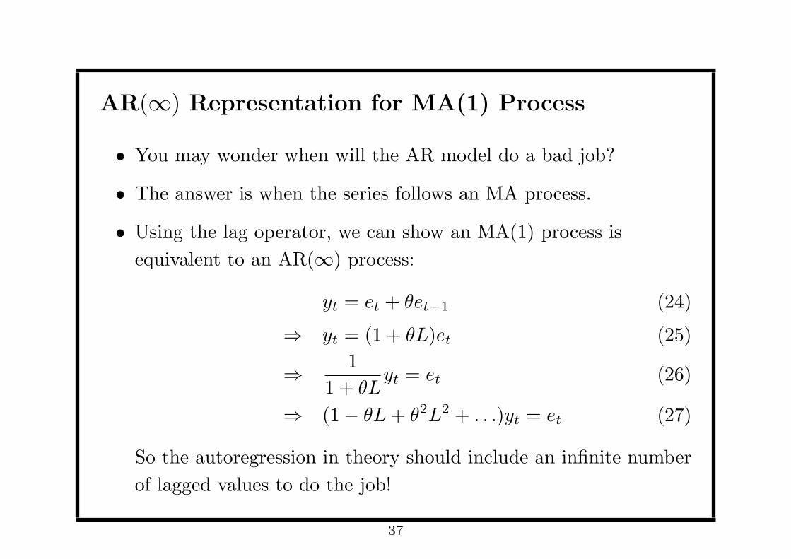
AR(∞) Representation for MA(1) Process
• You may wonder when will the AR model do a bad job?
• The answer is when the series follows an MA process.
• Using the lag operator, we can show an MA(1) process is
equivalent to an AR(∞) process:
yt = et + θet−1 (24)
⇒ yt = (1 + θL)et (25)
⇒ 1
1 + θLyt = et (26)
⇒ (1− θL+ θ2L2 + . . .)yt = et (27)
So the autoregression in theory should include an infinite number
of lagged values to do the job!
37

Lecture 4c: Forecasting
38

Big Picture
People use ARMA models mainly because their objective is to
obtaining forecasts for future values. It turns out conditional mean
plays a key role in finding the predicted values.
39

Review: Conditional Mean
Let X,Y be random variables, and c be a constant
E(c|X) = c (28)
E(cX|Y ) = cE(X|Y ) (29)
E(f(X)|X) = f(X) (30)
E(X) = EY [E(X|Y )] (law of iterated expectation) (31)
40

Theorem
• The best forecast (in terms of minimizing sum of squared
forecast error) for yt given yt−1, yt−2, . . . is the conditional mean
best forecast = E(yt|yt−1, yt−2, . . .)
• By construction, the forecasting error of using the conditional
mean is white noise
et ≡ yt − E(yt|yt−1, yt−2) ∼ white noise
• Proving this theorem requires the knowledge of the law of
iterated expectation, and is beyond the scope of this course.
41
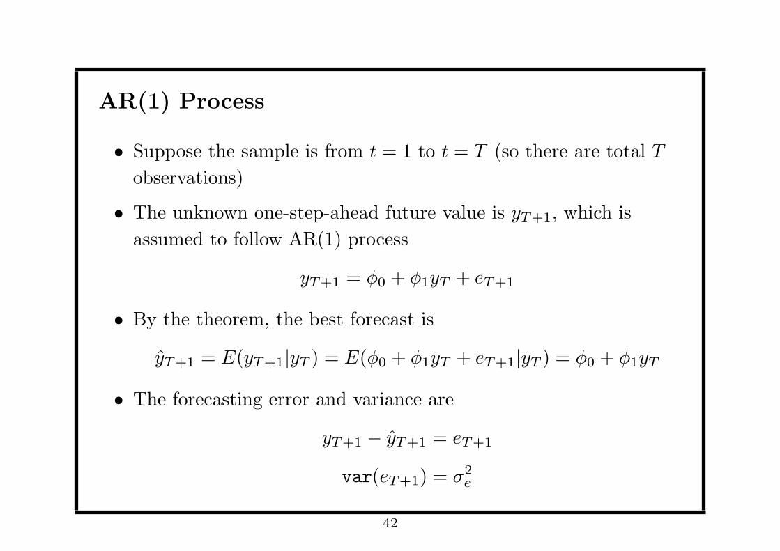
AR(1) Process
• Suppose the sample is from t = 1 to t = T (so there are total T
observations)
• The unknown one-step-ahead future value is yT+1, which is
assumed to follow AR(1) process
yT+1 = ϕ0 + ϕ1yT + eT+1
• By the theorem, the best forecast is
yT+1 = E(yT+1|yT ) = E(ϕ0 + ϕ1yT + eT+1|yT ) = ϕ0 + ϕ1yT
• The forecasting error and variance are
yT+1 − yT+1 = eT+1
var(eT+1) = σ2e
42
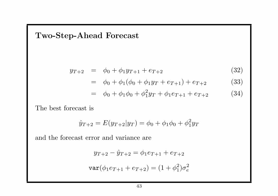
Two-Step-Ahead Forecast
yT+2 = ϕ0 + ϕ1yT+1 + eT+2 (32)
= ϕ0 + ϕ1(ϕ0 + ϕ1yT + eT+1) + eT+2 (33)
= ϕ0 + ϕ1ϕ0 + ϕ21yT + ϕ1eT+1 + eT+2 (34)
The best forecast is
yT+2 = E(yT+2|yT ) = ϕ0 + ϕ1ϕ0 + ϕ21yT
and the forecast error and variance are
yT+2 − yT+2 = ϕ1eT+1 + eT+2
var(ϕ1eT+1 + eT+2) = (1 + ϕ21)σ
2e
43

h-Step-Ahead Forecast
For the h-step-ahead future value, its best forecast and forecast
variance are
yT+h = E(yT+h|yT ) = ϕ0 + ϕ1ϕ0 + . . .+ ϕh−11 ϕ0 + ϕh
1yT (35)
var(yT+h − yT+h) = (1 + ϕ21 + . . .+ ϕ
2(h−1)1 )σ2
e (36)
44
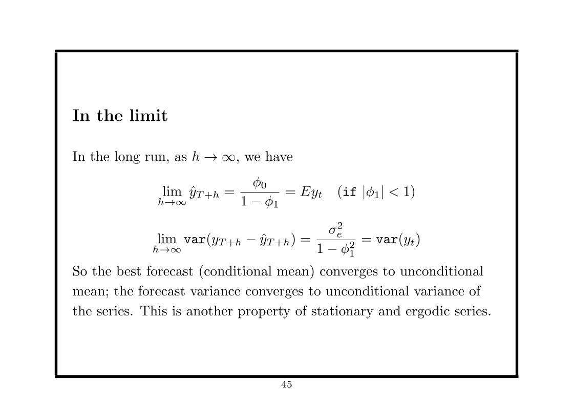
In the limit
In the long run, as h → ∞, we have
limh→∞
yT+h =ϕ0
1− ϕ1= Eyt (if |ϕ1| < 1)
limh→∞
var(yT+h − yT+h) =σ2e
1− ϕ21
= var(yt)
So the best forecast (conditional mean) converges to unconditional
mean; the forecast variance converges to unconditional variance of
the series. This is another property of stationary and ergodic series.
45

Intuition
The condition |ϕ1| < 1 ensures that the ergodicity holds. For an
ergodic series, two observations are almost independent if they are far
away from each other. That is the case for yT and yT+h when h → ∞(ie., yT becomes increasingly irrelevant for yT+h). As a result, the
conditional mean converges to unconditional mean.
46
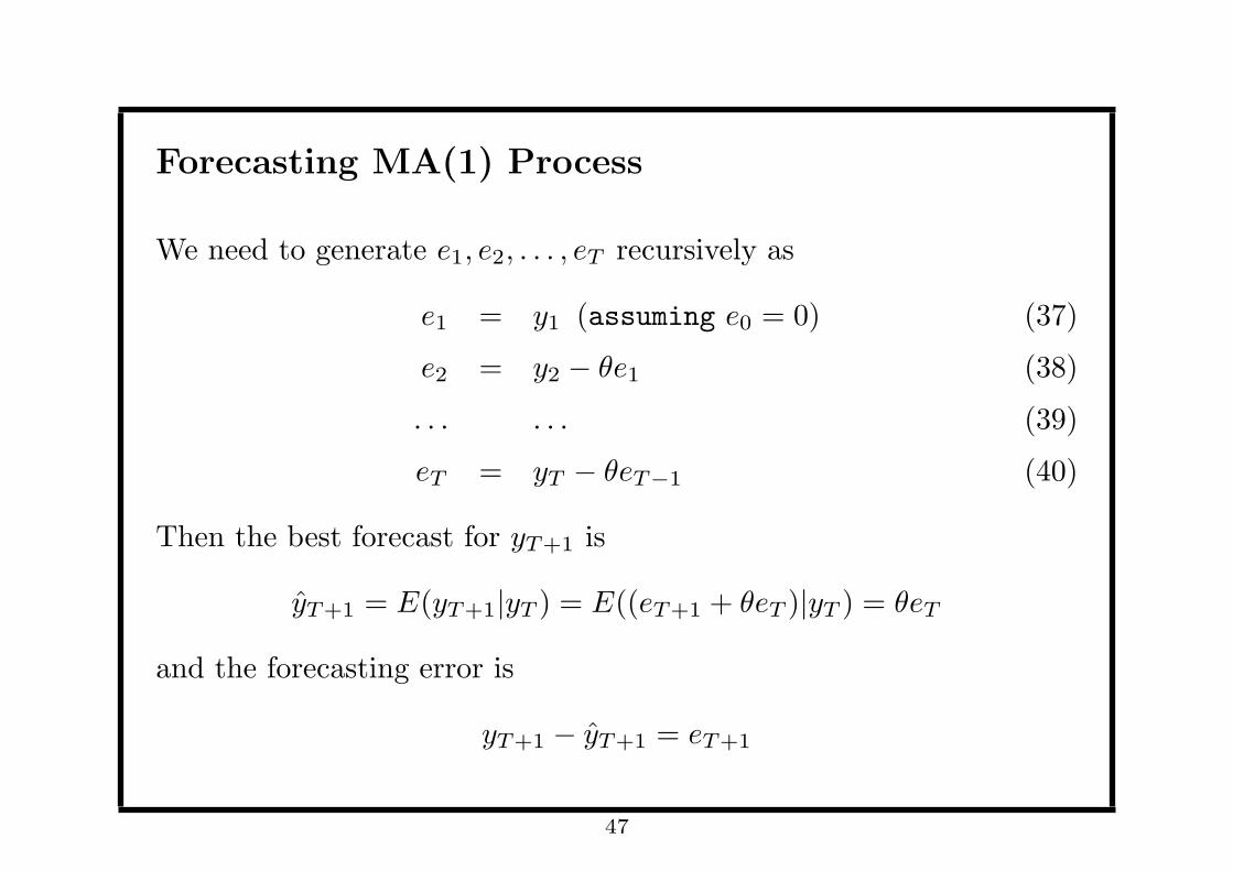
Forecasting MA(1) Process
We need to generate e1, e2, . . . , eT recursively as
e1 = y1 (assuming e0 = 0) (37)
e2 = y2 − θe1 (38)
. . . . . . (39)
eT = yT − θeT−1 (40)
Then the best forecast for yT+1 is
yT+1 = E(yT+1|yT ) = E((eT+1 + θeT )|yT ) = θeT
and the forecasting error is
yT+1 − yT+1 = eT+1
47

Two-Step-Ahead Forecast
yT+2 = eT+2 + θeT+1
It follows that the best forecast and forecasting variance are
yT+2 = E(eT+2 + θeT+1|yT ) = 0 = Eyt
var(yT+2 − yT+2) = (1 + θ2)σ2e = var(yt)
In this case the conditional mean converges to unconditional mean
very quickly. This makes sense because MA(1) process has extremely
short memory (recall that its acf is truncated after the first lag).
48

One More Thing
So far we assume the parameters ϕ and θ are known. In practice, we
use their estimates when computing the forecasts. For example, for
MA(1) process
yT+1 = θeT
49

What if
• So far we make strong assumption about the data generating
process: we assume the series follows AR or MA process. What if
this assumption is wrong? Without that assumption, what do we
get after we run an autoregression?
• It turns out autoregression will always give us the best linear
predictor (BLP) of yt given yt−1, yt−2, . . . . The BLP may and
may not be the best forecast; but it is the best linear forecast.
• The BLP is the best forecast if the conditional mean
E(yt|yt−1, yt−2, . . .) takes a linear form
BLP is best forecast if E(yt|yt−1, yt−2, . . .) = ϕ0+ϕ1yt−1+. . .
• If the conditional mean is a nonlinear function, BLP is not the
best forecast.
50
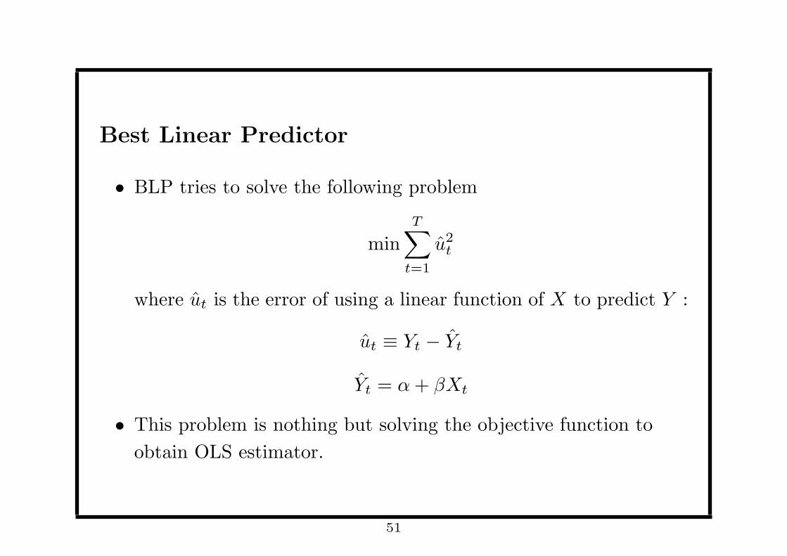
Best Linear Predictor
• BLP tries to solve the following problem
minT∑
t=1
u2t
where ut is the error of using a linear function of X to predict Y :
ut ≡ Yt − Yt
Yt = α+ βXt
• This problem is nothing but solving the objective function to
obtain OLS estimator.
51

Lecture 4d: Modeling US Annual Inflation Rate
52

Data
1. The annual data for consumer price index (CPI) from 1947 to
2013 are downloaded from
http://research.stlouisfed.org/fred2/
2. By definition, the inflation rate (INF) is the percentage change of
CPI, so is approximately computed as the log difference:
INFt ≡CPIt − CPIt−1
CPIt−1≈ log(CPIt)− log(CPIt−1)
53

CPI time series plot
Yearly U.S. CPI
Time
cpi
1950 1960 1970 1980 1990 2000 2010
5010
015
020
0
54
Remarks
• We see CPI is overall upward-trending (occasionally CPI went
down in a deflation)
• The trend implies that the mean (expected value) changes over
time
• So CPI is not stationary, and we cannot apply the ARMA model
to CPI
55
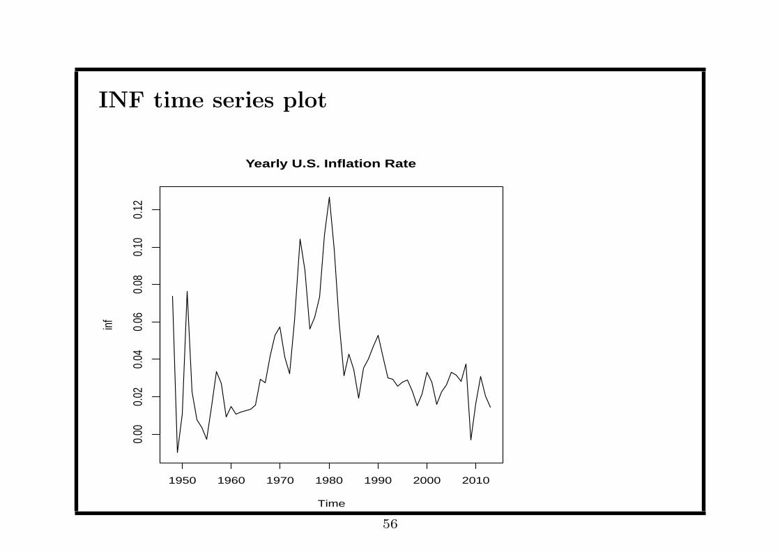
INF time series plot
Yearly U.S. Inflation Rate
Time
inf
1950 1960 1970 1980 1990 2000 2010
0.00
0.02
0.04
0.06
0.08
0.10
0.12
56

Remarks
• INF is not trending; the lesson is that taking difference may
remove trending behavior
• However, the INF series looks quite different before and after
early 1980s. That is when Paul Volcker was the chairman of
federal reserve, whose policy successfully ended the high levels of
inflation.
• We may conclude the whole series is not stationary due to the
structural break in 1980s. However, the subsample after 1982
seems stationary.
• So we can apply the ARMA model, but using the subsample
after 1982 only
57

Model Selection
• We use the modern approach that the final model is selected by
minimizing AIC among several candidates models.
• The AR(1) model (for subsample after 1982) is estimated using
the command arima(x = rinf, order = c(1, 0, 0))
where rinf is the after-1982 subset of INF.
• Then we try AR(2), AR(3) and ARMA(1,1) models. Their AIC
are all greater than AR(1) model. So AR(1) model is selected.
58
Test for Model Adequacy
• We can test the null hypothesis that AR(1) model is adequate by
testing the equivalent null hypothesis that the residual of AR(1)
model is white noise (serially uncorrelated)
• We use the command
Box.test(ar1$res, lag = 1, type = "Ljung")
to implement the Box-Ljung test with one lag. The p-value is
0.5664, greater than 0.05. So we cannot reject the null that the
AR(1) is adequate.
• The p-value for the Box-Ljung test with four lags is also greater
than 0.05.
• So we conclude that AR(1) model is adequate, in the sense that
all serial correlation in INF has been accounted for.
59

Equivalent Forms
• The same time series can be expressed as several equivalent
forms.
• For example, the standard form for the AR(1) process is
yt = ϕ0 + ϕ1yt−1 + et
• There is an equivalent “deviation-from-mean” form
yt = µ+ dt
dt = ϕ1dt−1 + et
µ ≡ ϕ0
1− ϕ1
where µ = E(yt) is the mean, dt ≡ yt − µ is the deviation, and
E(dt) = 0 by construction
60

“deviation-from-mean” form
1. Note that the deviation dt has zero mean.
2. Basically we can always rewrite an AR(1) process with nonzero
mean yt as the sum of the mean µ and a zero-mean deviation
process dt.
3. The serial correlation is captured by ϕ1, which remains
unchanged during the transformation
4. So without loss of generality, we can assume the series has zero
mean when developing the theory
61

Warning
1. The “intercept” reported by R command arima is µ, not ϕ0.
2. Therefore the selected AR(1) model for INF (after 1982) is
(INFt − 0.0297) = 0.4294(INFt−1 − 0.0297) + et
or equivalently
INFt = 0.01694682 + 0.4294INFt−1 + et
More explicitly,
µ = 0.0297
ϕ0 = 0.01694682
ϕ1 = 0.4294
62

Stationarity
Note that ϕ1 = 0.4294 < 1. So INF is indeed stationary after 1982.
63

Forecast
• The sample ends at year 2013, in which the inflation rate is
0.014553604.
• Mathematically, that means yT = 0.014553604
• The forecast for 2014 inflation rate is
INFT+1 = ϕ0 + ϕ1INFT
= 0.01694682 + 0.4294 ∗ 0.014553604
= 0.02319614
• Now you can use Fisher equation to forecast the nominal interest
rate, and make decision about whether or not to buy a house, etc
64

ML vs OLS
• By default, command arima uses the maximum likelihood (ML)
method to estimate the AR model.
• You may prefer OLS, which is more robust (because it makes no
distributional assumption), and can always gives us the best
linear predictor (BLP)
• The command to obtain the OLS estimate of the AR(1) model is
arima(rinf, order=c(1,0,0), method="CSS")
65

A more transparent way
• Still some people think of command arima as a black box.
• A more transparent way to estimate the AR model is to generate
the lagged value explicitly, and then run the OLS linear
regression.
• The R command to do that is
y = rinf[2:32]
y.lag1 = rinf[1:31]
lm(y~y.lag1)
• You can get ϕ0 directly this way.
66