lecture 5 6_7 - divide and conquer and method of solving recurrences
TRANSCRIPT

Lecture 5 : Divide & Conquer Approach & Methods of Solving
Recurrences
Jayavignesh T
Asst Professor
SENSE

Asymptotic Notations..

Asymptotic Notations..


Problems – Big Oh, Big Omega, Big Thetha
• First two functions are linear and hence have a lower order of growth than g(n) = n2, while the last one is quadratic and hence has the same order of growth as n2
• Functions n3 and 0.00001n3 are both cubic and hence have a higher order of growth than n2, and so has the fourth-degree polynomial n4 + n + 1

Problems – Big Oh, Big Omega, Big Thetha
• Ω(g(n)), stands for the set of all functions with a higher or same order of growth as g(n) (to within a constant multiple, as n goes to infinity).
• Θ(g(n)) is the set of all functions that have the same order of growth as g(n) (to within a constant multiple, as n goes to infinity). Every quadratic function an2 + bn + c with a > 0 is in Θ(n2).

Exercise

Divide-and-Conquer
• The most-well known algorithm design strategy:
1. Divide instance of problem into two or more smaller instances
2. Solve smaller instances recursively
(Base case: If the sub-problem sizes are small enough, solve the sub-problem in a straight forward or direct manner).
3. Obtain solution to original (larger) instance by combining these solutions
• Type of recurrence relation

Divide-and-Conquer

Divide-and-Conquer Technique (cont.)
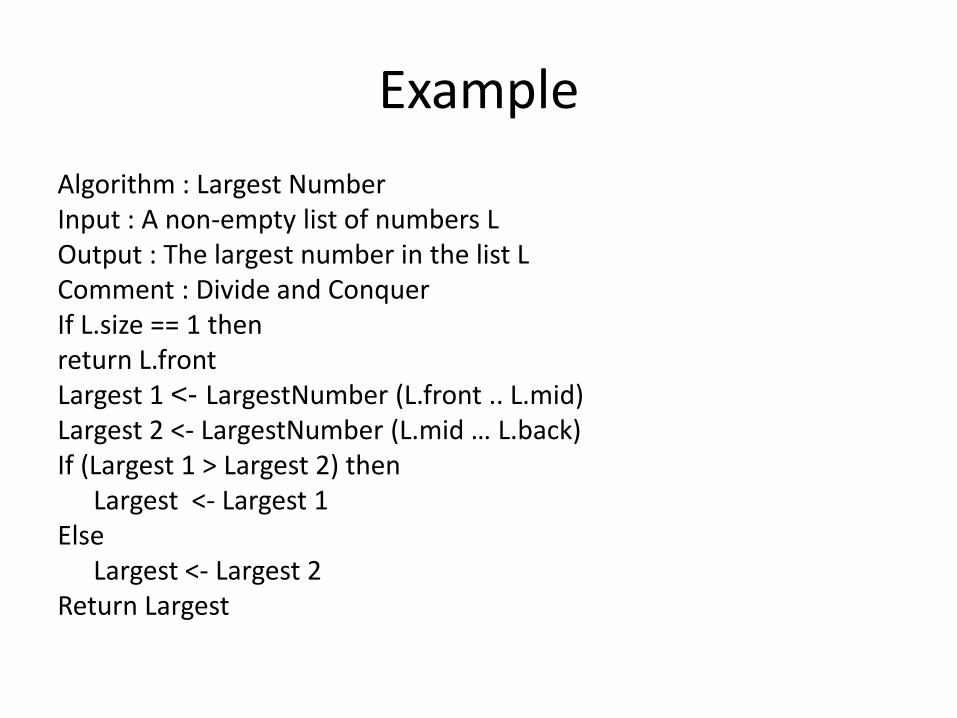
Example
Algorithm : Largest Number Input : A non-empty list of numbers L Output : The largest number in the list L Comment : Divide and Conquer If L.size == 1 then return L.front Largest 1 <- LargestNumber (L.front .. L.mid) Largest 2 <- LargestNumber (L.mid … L.back) If (Largest 1 > Largest 2) then Largest <- Largest 1 Else Largest <- Largest 2 Return Largest

Recurrence Relation
• Any problem can be solved either by writing recursive algorithm or by writing non-recursive algorithm.
• A recursive algorithm is one which makes a recursive call to itself with smaller inputs.
• We often use a recurrence relation to describe the running time of a recursive algorithm.
• Recurrence relations often arise in calculating the time and space complexity of algorithms.

Recurrence Relations contd..
• A recurrence relation is an equation or inequality that describes a function in terms of its value on smaller inputs or as a function of preceding (or lower) terms.
1. Base step:
– 1 or more constant values to terminate recurrence.
– Initial conditions or base conditions.
2. Recursive steps:
– To find new terms from the existing (preceding) terms.
– The recurrence compute next sequence from the k preceding values .
– Recurrence relation (or recursive formula).
– This formula refers to itself, and the argument of the formula must be on smaller values (close to the base value).

Recurrence Formula : Ex 1 Fibonacci Sequence
• Recurrence has one or more initial conditions and a recursive formula, known as recurrence relation.
• Fibonacci sequence f0,f1,f2…. can be defined by the recurrence relation
• (Base Step) – The given recurrence says that if n=0 then f0=1 and if n=1
then f1=1. – These two conditions (or values) where recursion does
not call itself is called a initial conditions (or Base conditions).

Ex : Fibonacci Sequence contd..
• (Recursive step): This step is used to find new terms f2,f3….from the existing (preceding) terms, by using the formula
• This formula says that “by adding two previous sequence (or term) we can get the next term”.

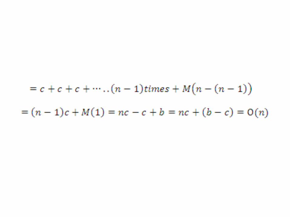
Ex 2 : Factorial Computation

Recurrence Relation for Factorial Computation
• M(n)
– denoted the number of multiplication required to execute the n!
• Initial condition
– M(1) = 0 ; BASE Step
• n > 1
– Performs 1 Multiplication + FACT recursively called with input n-1

Recurrence Relation for Factorial Computation

Example 3

Example 3
• Let T(n) denotes recurrence relation - number of times the statement x=x+1 is executed in the algorithm
x+1 to be executed T(n/2) additional times

Example 3
Performs TWO recursive calls each with the parameter at line 4, and some constant number of basic operations

22
Recurrences and Running Time
• An equation or inequality that describes a function in terms of
its value on smaller inputs.
T(n) = T(n-1) + n
• Recurrences arise when an algorithm contains recursive calls to
itself
• What is the actual running time of the algorithm?
• Need to solve the recurrence
– Find an explicit formula of the expression
– Bound the recurrence by an expression that involves n

23
Recurrent Algorithms - BINARY-SEARCH
• for an ordered array A, finds if x is in the array A[lo…hi]
Alg.: BINARY-SEARCH (A, lo, hi, x)
if (lo > hi)
return FALSE
mid (lo+hi)/2
if x == A[mid]
return TRUE
if ( x < A[mid] )
BINARY-SEARCH (A, lo, mid-1, x)
if ( x > A[mid] )
BINARY-SEARCH (A, mid+1, hi, x)
12 11 10 9 7 5 3 2
1 2 3 4 5 6 7 8
mid lo hi

24
Example
• A[8] = {1, 2, 3, 4, 5, 7, 9, 11}
– lo = 1 hi = 8 x = 7
mid = 4, lo = 5, hi = 8
mid = 6, A[mid] = x Found! 11 9 7 5 4 3 2 1
11 9 7 5 4 3 2 1
1 2 3 4 5 6 7 8
8 7 6 5

25
Another Example
• A[8] = {1, 2, 3, 4, 5, 7, 9, 11}
– lo = 1 hi = 8 x = 6
mid = 4, lo = 5, hi = 8
mid = 6, A[6] = 7, lo = 5, hi = 5 11 9 7 5 4 3 2 1
11 9 7 5 4 3 2 1
1 2 3 4 5 6 7 8
11 9 7 5 4 3 2 1 mid = 5, A[5] = 5, lo = 6, hi = 5 NOT FOUND!
11 9 7 5 4 3 2 1
low high
low
low high
high
26
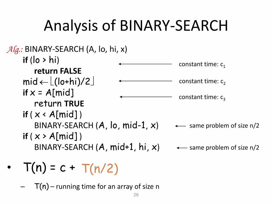
Analysis of BINARY-SEARCH
Alg.: BINARY-SEARCH (A, lo, hi, x) if (lo > hi) return FALSE mid (lo+hi)/2 if x = A[mid] return TRUE if ( x < A[mid] ) BINARY-SEARCH (A, lo, mid-1, x) if ( x > A[mid] ) BINARY-SEARCH (A, mid+1, hi, x)
• T(n) = c +
– T(n) – running time for an array of size n
constant time: c2
same problem of size n/2
same problem of size n/2
constant time: c1
constant time: c3
T(n/2)

27
Methods for Solving Recurrences
• Iteration method
–(unrolling and summing)
• Substitution method
• Recursion tree method
• Master method

• Iteration Method : – Converts the recurrence into a summation and then relies
on techniques for bounding summations to solve the recurrence.
• Substitution Method : – Guess a asymptotic bound and then use mathematical
induction to prove our guess correct.
• Recursive Tree Method : – Graphical depiction of the entire set of recursive
invocations to obtain guess and verify by substitution method.
• Master Method : – Cookbook method for determining asymptotic solutions to
recurrences of a specific form.
Method of Solving Recurrences
29
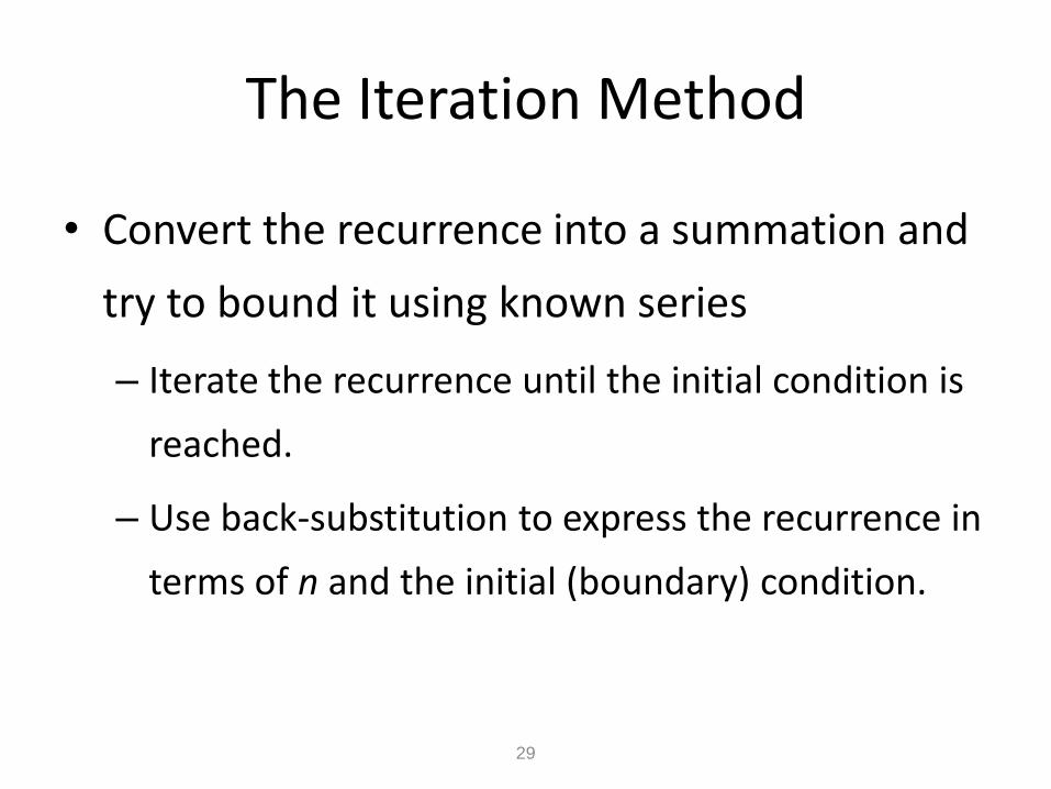
The Iteration Method
• Convert the recurrence into a summation and
try to bound it using known series
– Iterate the recurrence until the initial condition is
reached.
– Use back-substitution to express the recurrence in
terms of n and the initial (boundary) condition.

Iteration Method - Example 1

Iteration Method - Example 1

Binary Search – Running Time T(n) = c + T(n/2)

Binary Search – Running Time T(n) = c + T(n/2)
T(n) = c + T(n/2)
= c + c + T(n/4)
= c + c + c + T(n/8)
Assume n = 2k
T(n) = c + c + … + c + T(1) = c log2 n + T(1)
= O(log n)
k times
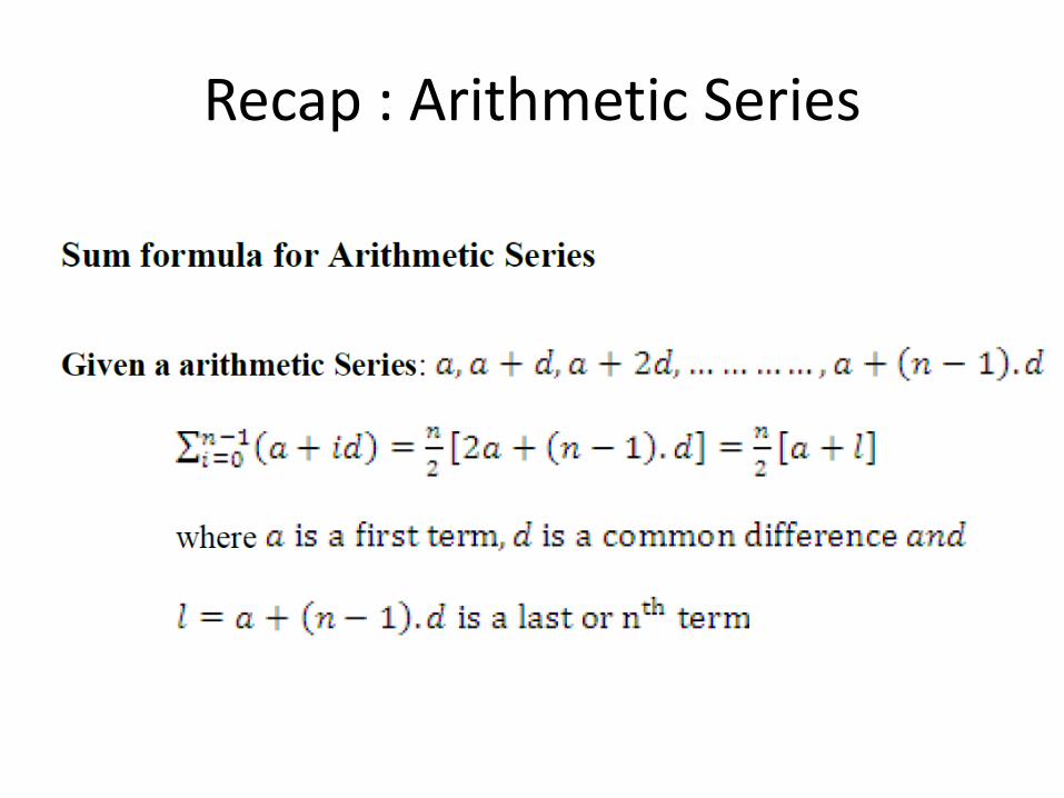
Recap : Arithmetic Series

Recap : Geometric Series

Problem 3


Iteration method

Iteration method

Example Recurrences
• T(n) = T(n-1) + n – Recursive algorithm that loops through the input to eliminate one item • T(n) = T(n/2) + c – Recursive algorithm that halves the input in one step • T(n) = T(n/2) + n – Recursive algorithm that halves the input but must examine every item in the input • T(n) = 2T(n/2) + 1 – Recursive algorithm that splits the input into 2 halves and does a constant amount of other work • T(n) = T(n/3) + T(2n/3) + n

Logarithmic Formulae - Revisit
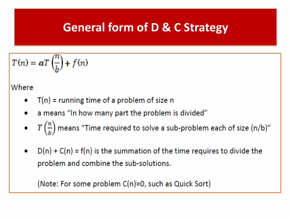
General form of D & C Strategy
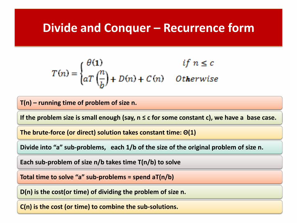
Divide and Conquer – Recurrence form
T(n) – running time of problem of size n.
If the problem size is small enough (say, n ≤ c for some constant c), we have a base case.
The brute-force (or direct) solution takes constant time: Θ(1)
Divide into “a” sub-problems, each 1/b of the size of the original problem of size n.
Each sub-problem of size n/b takes time T(n/b) to solve
Total time to solve “a” sub-problems = spend aT(n/b)
D(n) is the cost(or time) of dividing the problem of size n.
C(n) is the cost (or time) to combine the sub-solutions.
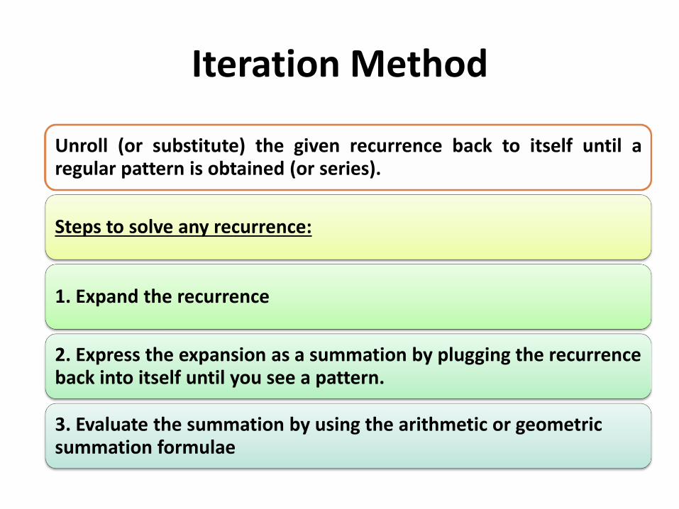
Iteration Method
Unroll (or substitute) the given recurrence back to itself until a regular pattern is obtained (or series).
Steps to solve any recurrence:
1. Expand the recurrence
2. Express the expansion as a summation by plugging the recurrence back into itself until you see a pattern.
3. Evaluate the summation by using the arithmetic or geometric summation formulae

Recursion Tree Method
A convenient way to visualize what happens when a recurrence is iterated.
Pictorial representation of how recurrences is divided till boundary condition
Used to solve a recurrence of the form

Steps for solving a recurrence using recursion Tree:
Step1: Make a recursion tree for a given recurrence as follow:
a) Put the value of f(n) at root node of a tree and make “a” no of child node of this root value f(n).

Steps for solving a recurrence using recursion Tree:

Steps for solving a recurrence using recursion Tree:
b) Find the value of T(n/b)

c) Expand a tree one more level (i.e. up to (at
least) 2 levels)
Steps for solving a recurrence using recursion Tree:

Recursive Tree method
Step2: (a) Find per level cost of a tree
Per level cost = Sum of the cost of each node at that level
Ex : Per level cost at level 1 = Row Sum
Total (final) cost of the tree = Sum of costs of all these levels. – Column Sum

Example 1
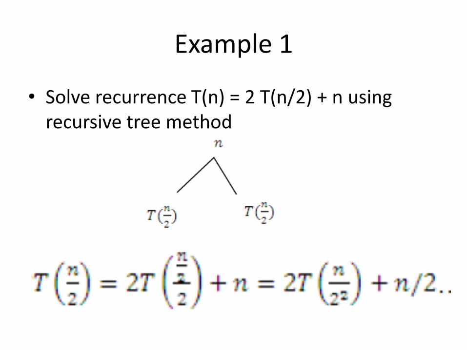
• Solve recurrence T(n) = 2 T(n/2) + n using recursive tree method
Example 1
• Solve recurrence T(n) = 2 T(n/2) + n using recursive tree method

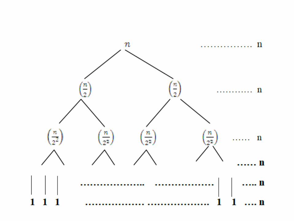

Per level cost = Sum of cost at each level = Row sum
Ex: Depth 2
Total cost is the sum of the costs of all levels (called Column sum), which gives the solution of a given Recurrence

To find Total number of terms -> Height of the tree
k represents the height of tree = log2n
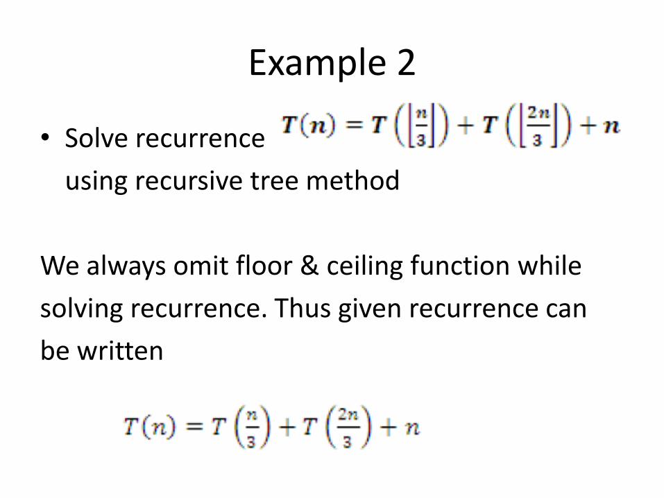
Example 2
• Solve recurrence
using recursive tree method
We always omit floor & ceiling function while
solving recurrence. Thus given recurrence can
be written

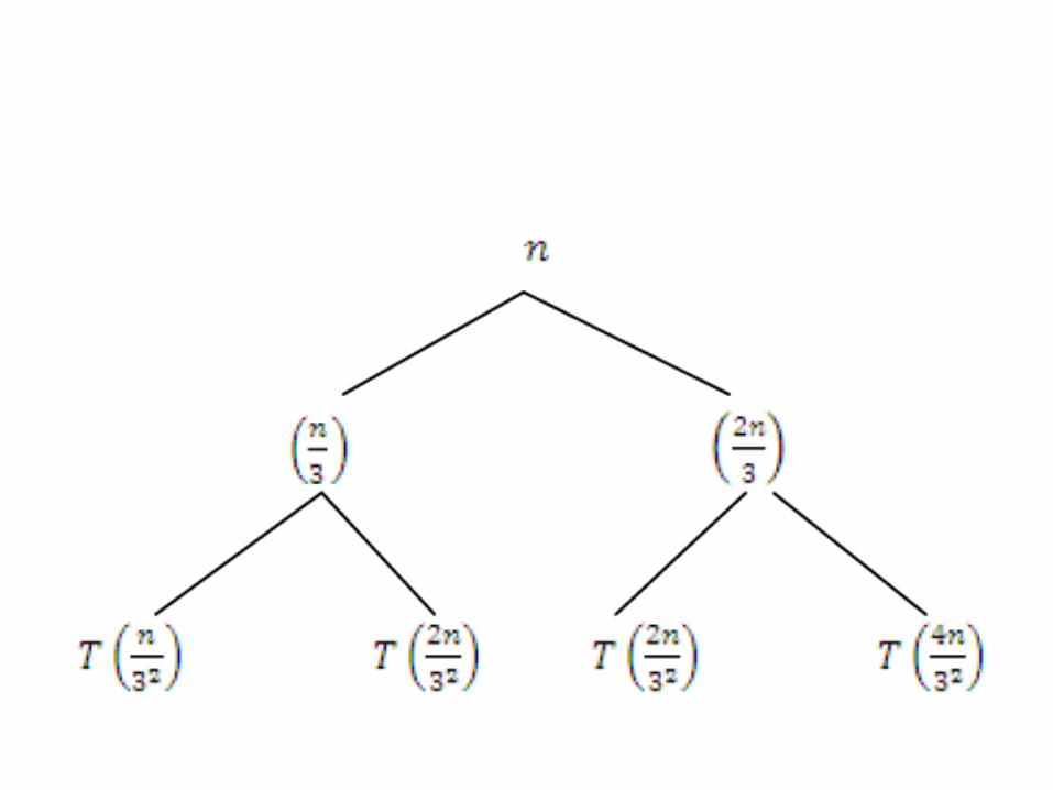

In this way, you can extend a tree up to Boundary condition
(when problem size becomes 1)


Tower of Hanoi Problem

Example 3
• To move n disks (n > 1) from peg A to C
– Move (n-1) disks recursively from peg A to peg B using peg C as auxillary = M(n-1) moves
– Move the nth disk directly (last) from peg A to peg C = 1 Move
– Move (n-1) disk recursively from peg B to peg C using peg A as auxillary = M(n-1) moves

Recurrence Relation for the Towers of Hanoi
Given: T(1) = 1
T(n) = 2 T( n-1 ) +1
N No.Moves
1 1
2 3
3 7
4 15
5 31
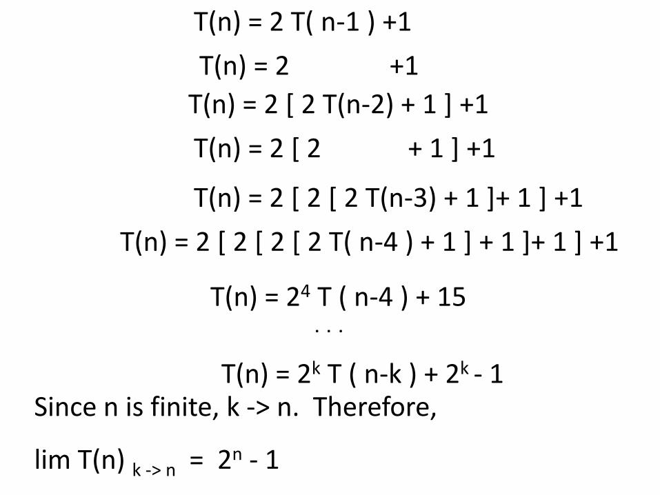
T(n) = 2 T( n-1 ) +1
T(n) = 2 +1
T(n) = 2 [ 2 T(n-2) + 1 ] +1
T(n) = 2 [ 2 + 1 ] +1
T(n) = 2 [ 2 [ 2 T(n-3) + 1 ]+ 1 ] +1
T(n) = 2 [ 2 [ 2 [ 2 T( n-4 ) + 1 ] + 1 ]+ 1 ] +1
. . .
T(n) = 24 T ( n-4 ) + 15
T(n) = 2k T ( n-k ) + 2k - 1
Since n is finite, k -> n. Therefore,
lim T(n) k -> n = 2n - 1

Tower of Hanoi Problem


Tower of Hanoi - Recursion
TOWER(n, A, C, B) {
TOWER(n-1, A, B, C);
Move(A, C);
TOWER(n-1, B, C, A) }
if n<1 return;

Merge Sort
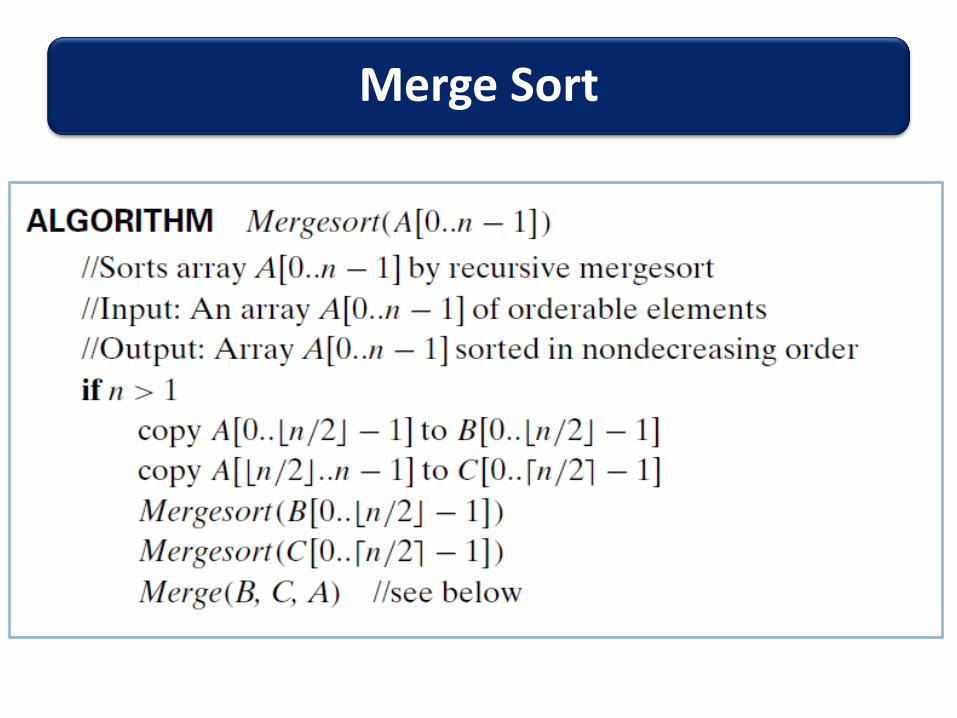
Merge Sort

Merge Sort


Quick Sort
Divide:
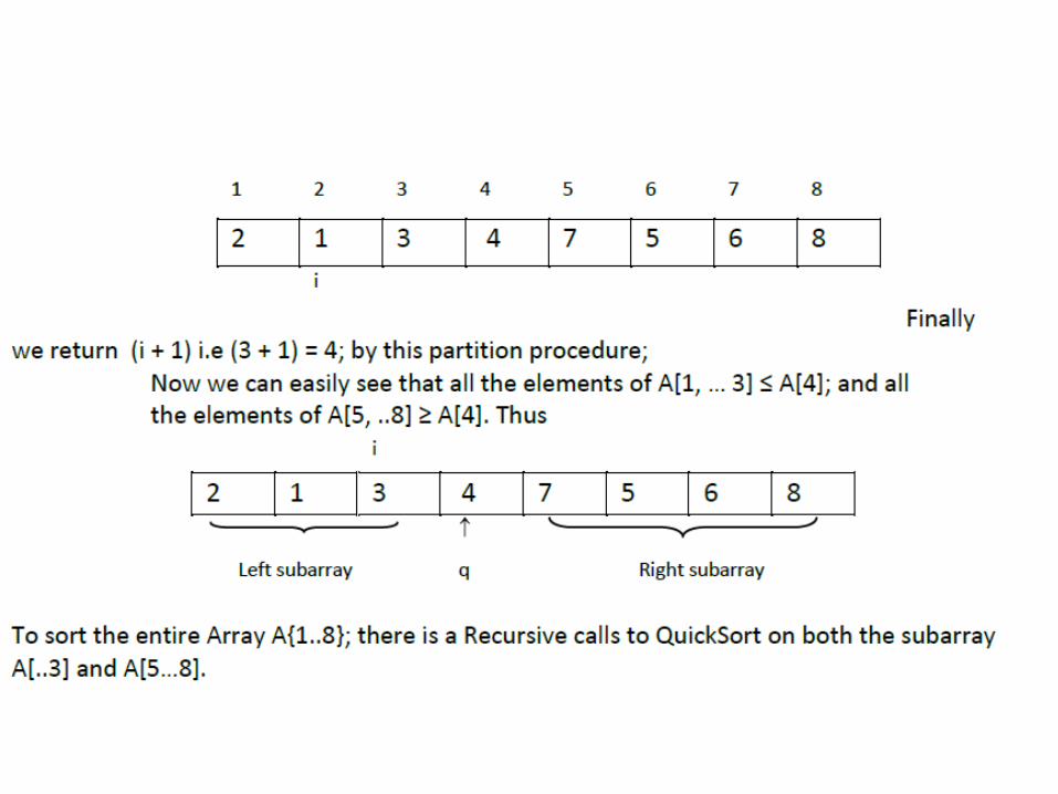
• A [p. . r] is partitioned (rearranged) into A [p..q-1] and A [q+1,..r],
• Each element in the left subarray A[p…q-1] is ≤ A [q] and
• A[q] is ≤ each element in the right subarray A[q+1…r]
• PARTITION procedure (Divide Step); returns the index q, where the array gets partitioned.
Conquer:
• These two subarray A [p…q-1] and A [q+1..r] are sorted by recursive calls to QUICKSORT.
Combine:
• Since the subarrays are sorted in place, so there is no need to combine the subarrays.

Quick Sort
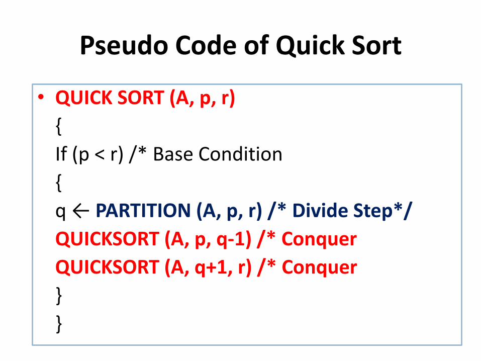
Pseudo Code of Quick Sort
• QUICK SORT (A, p, r)
{
If (p < r) /* Base Condition
{
q ← PARTITION (A, p, r) /* Divide Step*/
QUICKSORT (A, p, q-1) /* Conquer
QUICKSORT (A, q+1, r) /* Conquer
}
}
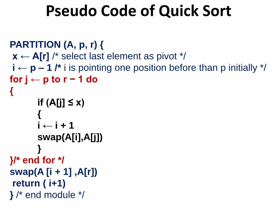
Pseudo Code of Quick Sort
PARTITION (A, p, r) {
x ← A[r] /* select last element as pivot */
i ← p – 1 /* i is pointing one position before than p initially */
for j ← p to r − 1 do
{
if (A[j] ≤ x)
{
i ← i + 1
swap(A[i],A[j])
}
}/* end for */
swap(A [i + 1] ,A[r])
return ( i+1)
} /* end module */


Best Case

Worst Case

• T(n) = T(n-1) + T(0) + cn

Average Case

QUICK-SORT
Fastest known Sorting algorithm in practice
Running time of Quick-Sort depends on the nature of its input data
Worst case (when input array is already sorted) O(n2)
Best Case (when input data is not sorted) Ω(nlogn)
Average Case (when input data is not sorted & Partition of array is not unbalanced as worst case) : Θ(nlogn)

91
Master’s method
• “Cookbook” for solving recurrences of the form:
where, a ≥ 1, b > 1, and f(n) > 0
Idea: compare f(n) with nlogba
• f(n) is asymptotically smaller or larger than nlogba by a
polynomial factor n
• f(n) is asymptotically equal with nlogba
)()( nfb
naTnT

93
Master’s method
• “Cookbook” for solving recurrences of the form:
where, a ≥ 1, b > 1, and f(n) > 0
Case 1: if f(n) = O(nlogba -) for some > 0, then: T(n) = (nlog
ba)
Case 2: if f(n) = (nlogba), then: T(n) = (nlog
ba lgn)
Case 3: if f(n) = (nlogba +) for some > 0, and if
af(n/b) ≤ cf(n) for some c < 1 and all sufficiently large n, then:
T(n) = (f(n))
)()( nfb
naTnT
regularity condition

94
Examples
T(n) = 2T(n/2) + n
a = 2, b = 2, log22 = 1
Compare nlog2
2 with f(n) = n
f(n) = (n) Case 2
T(n) = (nlgn)

95
Examples
T(n) = 2T(n/2) + n2
a = 2, b = 2, log22 = 1
Compare n with f(n) = n2
f(n) = (n1+) Case 3 verify regularity cond.
a f(n/b) ≤ c f(n)
2 n2/4 ≤ c n2 c = ½ is a solution (c<1)
T(n) = (n2)
96
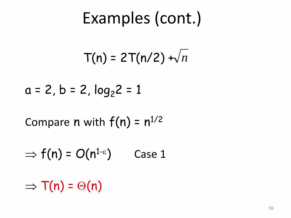
Examples (cont.)
T(n) = 2T(n/2) +
a = 2, b = 2, log22 = 1
Compare n with f(n) = n1/2
f(n) = O(n1-) Case 1
T(n) = (n)
n

97
Examples
T(n) = 2T(n/2) + nlgn
a = 2, b = 2, log22 = 1
• Compare n with f(n) = nlgn
– seems like case 3 should apply
• f(n) must be polynomially larger by a factor of n
• In this case it is only larger by a factor of lgn

98
Examples
T(n) = 3T(n/4) + nlgn
a = 3, b = 4, log43 = 0.793
Compare n0.793 with f(n) = nlgn
f(n) = (nlog4
3+) Case 3
Check regularity condition:
3(n/4)lg(n/4) ≤ (3/4)nlgn = c f(n),
c=3/4
T(n) = (nlgn)
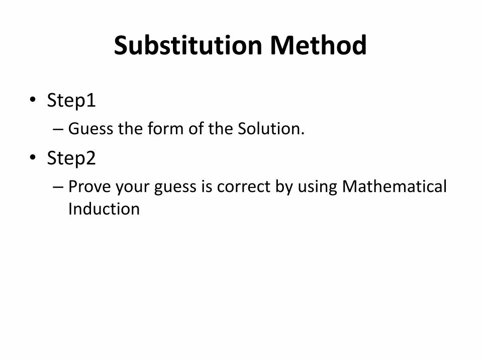
Substitution Method
• Step1
– Guess the form of the Solution.
• Step2
– Prove your guess is correct by using Mathematical Induction

Mathematical Induction
• Proof by using Mathematical Induction of a given statement (or formula), defined on the positive integer N, consists of two steps:
1. (Base Step): Prove that S(1) is true
2. (Inductive Step): Assume that S(n) is true, and prove that S(n+1) is true for all n>=1

Mathematical Induction - Example

Mathematical Induction - Example

Substitution method
• Guess a solution – T(n) = O(g(n)) – Induction goal: apply the definition of the
asymptotic notation • T(n) ≤ c g(n), for some c > 0 and n ≥ n0 – Induction hypothesis: T(k) ≤ c g(k) for all k < n
(strong induction) • Prove the induction goal – Use the induction hypothesis to find some
values of the constants c and n0 for which the induction goal holds
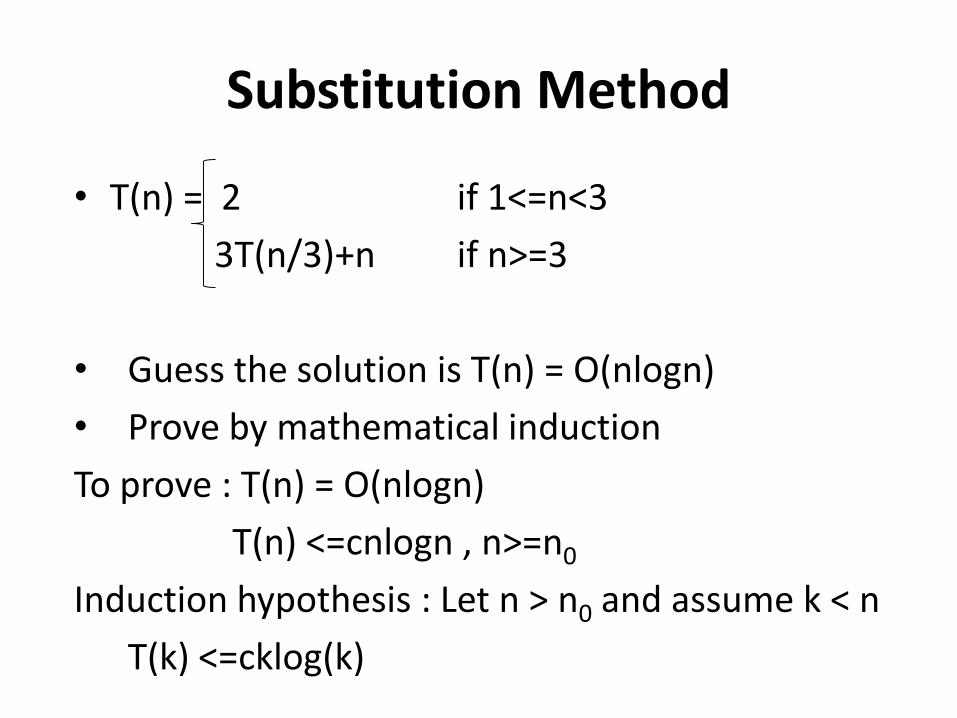
Substitution Method
• T(n) = 2 if 1<=n<3
3T(n/3)+n if n>=3
• Guess the solution is T(n) = O(nlogn)
• Prove by mathematical induction
To prove : T(n) = O(nlogn)
T(n) <=cnlogn , n>=n0
Induction hypothesis : Let n > n0 and assume k < n
T(k) <=cklog(k)

Substitution method
• Let’s take k = (n/3), T(n/3) <= c(n/3) log (n/3)
• To show T(n) <=cnlogn
T(n) = 3T(n/3) + n ( By recurrence for T)
T(n) = 3c(n/3)log(n/3) + n (By Induction hypothesis)
T(n) = cn(log n -1) + n
T(n) = cnlogn – cn + n
• To obtain T(n) <=cnlogn we need to have –cn+n <=0 , so c >=1 Induction step is cleared
• To determine n0, base step T(n0) <=cn0(logn0)
Advantages of Divide and Conquer
• Solving difficult problems
• Algorithm Efficiency
– Size n/b at each stage
• Parallelism
– Sub problems – multiprocessor
• Memory Access
– Make efficient use of memory cache

Disadvantages of D & C
• Recursion is slow
• Overhead of repeated subroutine calls
• With large recursive base cases, overhead can be become negligible