lecture 5 - information theory - masaryk university · jan bouda (fi mu) lecture 5 - information...

Lecture 5 - Information theory

Jan Bouda

FI MU

May 18, 2012

Jan Bouda (FI MU) Lecture 5 - Information theory May 18, 2012 1 / 42

Part I

Uncertainty and entropy


Uncertainty

Given a random experiment it is natural to ask how uncertain we areabout an outcome of the experiment.Compare two experiments - tossing an unbiased coin and throwing afair six-sided dice. First experiment attains two outcomes and thesecond experiment has six possible outcomes. Both experiments havethe uniform probability distribution. Our intuition says that we aremore uncertain about an outcome of the second experiment.Let us compare tossing of an ideal coin and a binary message sourceemitting 0 and 1 both with probability 1/2. Intuitively we shouldexpect that the uncertainty about an outcome of each of theseexperiments is the same. Therefore the uncertainty should be basedonly on the probability distribution and not on the concrete samplespace.Therefore, the uncertainty about a particular random experiment canbe specified as a function of the probability distribution{p1, p2, . . . , pn} and we will denote it as H(p1, p2, . . . , pn).Jan Bouda (FI MU) Lecture 5 - Information theory May 18, 2012 3 / 42

Uncertainty - requirements

1 Let us fix the number of outcomes of an experiment and compare theuncertainty of different probability distributions. Natural requirementis that the most uncertain is the experiment with the uniformprobability distribution, i.e. H(p1, . . . pn) is maximal forp1 = · · · = pn = 1/n.

2 Permutation of probability distribution does not change theuncertainty, i.e. for any permutation π : {1 . . . n} → {1 . . . n} it holdsthat H(p1, p2, . . . , pn) = H(pπ(1), pπ(2) . . . , pπ(n)).

3 Uncertainty should be nonnegative and equals to zero if and only ifwe are sure about the outcome of the experiment.H(p1, p2, . . . , pn) ≥ 0 and it is equal if and only of pi = 1 for some i .

4 If we include into an experiment an outcome with zero probability, thisdoes not change our uncertainty, i.e. H(p1, . . . , pn, 0) = H(p1, . . . , pn)


Uncertainty - requirements

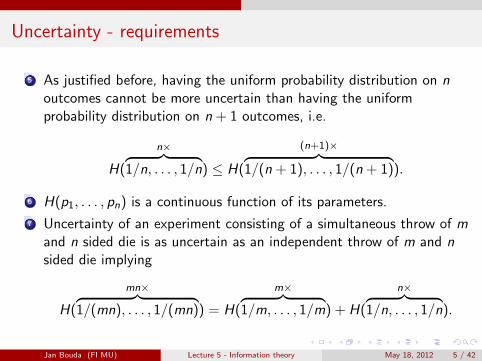
5 As justified before, having the uniform probability distribution on noutcomes cannot be more uncertain than having the uniformprobability distribution on n + 1 outcomes, i.e.

H(

n×︷︸︸︷1/n, . . . , 1/n) ≤ H(

(n+1)×︷︸︸︷1/(n + 1), . . . , 1/(n + 1)).

6 H(p1, . . . , pn) is a continuous function of its parameters.

7 Uncertainty of an experiment consisting of a simultaneous throw of mand n sided die is as uncertain as an independent throw of m and nsided die implying

H(

mn×︷︸︸︷1/(mn), . . . , 1/(mn)) = H(

m×︷︸︸︷1/m, . . . , 1/m) + H(

n×︷︸︸︷1/n, . . . , 1/n).


Entropy and uncertainty

8 Let us consider a random choice of one of n + m balls, m being redand n being blue. Let p =

∑mi=1 pi be the probability that a red ball

is chosen and q =∑m+n

i=m+1 pi be the probability that a blue one ischosen. Then the uncertainty which ball is chosen is the uncertaintywhether red of blue ball is chosen plus weighted uncertainty that aparticular ball is chosen provided blue/red ball was chosen. Formally,

H(p1, . . . , pm, pm+1, . . . , pm+n) =

=H(p, q) + pH

(p1

p, . . . ,

pm

p

)+ qH

(pm+1

q, . . . ,

pm+n

q

).

(1)

It can be shown that any function satisfying Axioms 1− 8 is of the form

H(p1, . . . , pm) = −(loga 2)m∑i=1

pi log2 pi (2)

showing that the function is defined uniquely up to multiplication by aconstant, which effectively changes only the base of the logarithm.


Entropy and uncertainty

Alternatively, we may show that the function H(p1, . . . , pm) is uniquelyspecified through axioms

1 H(1/2, 1/2) = 1.

2 H(p, 1− p) is a continuous function of p.

3 H(p1, . . . , pm) = H(p1 + p2, p3, . . . , pm) + (p1 + p2)H( p1p1+p2

, p2p1+p2

)

as in Eq. (2).


Entropy

The function H(p1, . . . , pn) we informally introduced is called the (Shannon)entropy and, as justified above, it measures our uncertainty about anoutcome of an experiment.

Definition

Let X be a random variable with probability distribution p(x). Then the(Shannon) entropy of the random variable X is defined as

H(X ) = −∑

x∈Im(X )

p(X = x) log P(X = x).

In the definition we use the convention that 0 log 0 = 0, what is justified bylimx→0 x log x = 0. Alternatively, we may sum only over nonzeroprobabilities.As explained above, all required properties are independent ofmultiplication by a constant what changes the base of the logarithm in thedefinition of the entropy. Therefore, in the rest of this part we will uselogarithm without explicit base. In case we want to measure information inbits, we should use logarithm base 2.


Entropy

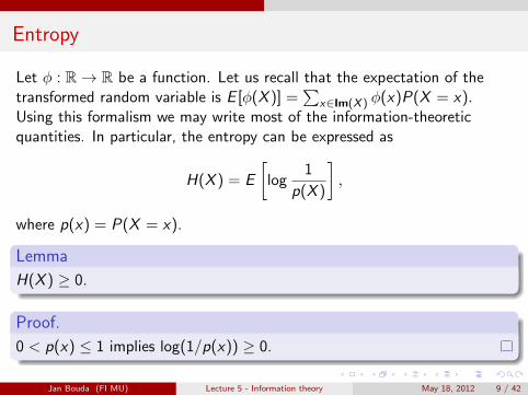
Let φ : R→ R be a function. Let us recall that the expectation of thetransformed random variable is E [φ(X )] =

∑x∈Im(X ) φ(x)P(X = x).

Using this formalism we may write most of the information-theoreticquantities. In particular, the entropy can be expressed as

H(X ) = E

[log

1

p(X )

],

where p(x) = P(X = x).

Lemma

H(X ) ≥ 0.

Proof.

0 < p(x) ≤ 1 implies log(1/p(x)) ≥ 0.


Part II

Joint and Conditional entropy


Joint entropy

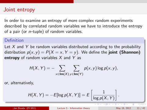
In order to examine an entropy of more complex random experimentsdescribed by correlated random variables we have to introduce the entropyof a pair (or n–tuple) of random variables.

Definition

Let X and Y be random variables distributed according to the probabilitydistribution p(x , y) = P(X = x ,Y = y). We define the joint (Shannon)entropy of random variables X and Y as

H(X ,Y ) = −∑

x∈Im(X )

∑y∈Im(Y )

p(x , y) log p(x , y),

or, alternatively,

H(X ,Y ) = −E [log p(X ,Y )] = E

[1

log p(X ,Y )

].


Conditional entropy

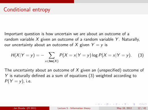
Important question is how uncertain we are about an outcome of arandom variable X given an outcome of a random variable Y . Naturally,our uncertainty about an outcome of X given Y = y is

H(X |Y = y) = −∑

x∈Im(X )

P(X = x |Y = y) log P(X = x |Y = y). (3)

The uncertainty about an outcome of X given an (unspecified) outcome ofY is naturally defined as a sum of equations (3) weighted according toP(Y = y), i.e.


Conditional Entropy

Definition

Let X and Y be random variables distributed according to the probabilitydistribution p(x , y) = P(X = x ,Y = y). Let us denotep(x |y) = P(X = x |Y = y). The conditional entropy of X given Y is

H(X |Y ) =∑

y∈Im(Y )

p(y)H(X |Y = y) =

=−∑

y∈Im(Y )

p(y)∑

x∈Im(X )

p(x |y) log p(x |y) =

=−∑

x∈Im(X )

∑y∈Im(Y )

p(x , y) log p(x |y)

=− E [log p(X |Y )].

(4)


Conditional Entropy

Using the previous definition we may raise the question how muchinformation we learn on average about X given an outcome of Y .Naturally, we may interpret it as the decrease of our uncertainty about Xwhen we learn outcome of Y , i.e. H(X )− H(X |Y ). Analogously, theamount of information we obtain when we learn the outcome of X isH(X ).

Theorem (Chain rule of conditional entropy)

H(X ,Y ) = H(Y ) + H(X |Y ).


Chain rule of conditional entropy

Proof.

H(X ,Y ) =−∑

x∈Im(X )

∑y∈Im(Y )

p(x , y) log p(x , y) =

=−∑

x∈Im(X )

∑y∈Im(Y )

p(x , y) log[p(y)p(x |y)] =

=−∑

x∈Im(X )y∈Im(Y )

p(x , y) log p(y)−∑


p(x , y) log p(x |y) =

=−∑

y∈Im(Y )

p(y) log p(y)−∑



=H(Y ) + H(X |Y ).

(5)


Part III

Relative Entropy and Mutual Information


Relative entropy

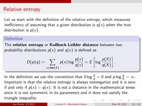
Let us start with the definition of the relative entropy, which measuresinefficiency of assuming that a given distribution is q(x) when the truedistribution is p(x).

Definition

The relative entropy or Kullback-Leibler distance between twoprobability distributions p(x) and q(x) is defined as

D(p‖q) =∑

x∈Im(X )

p(x) logp(x)

q(x)= E

[log

p(X )

q(X )

].

In the definition we use the convention that 0 log 0q = 0 and p log p

0 =∞.Important is that the relative entropy is always nonnegative and it is zeroif and only if p(x) = q(x). It is not a distance in the mathematical sensesince it is not symmetric in its parameters and it does not satisfy thetriangle inequality.


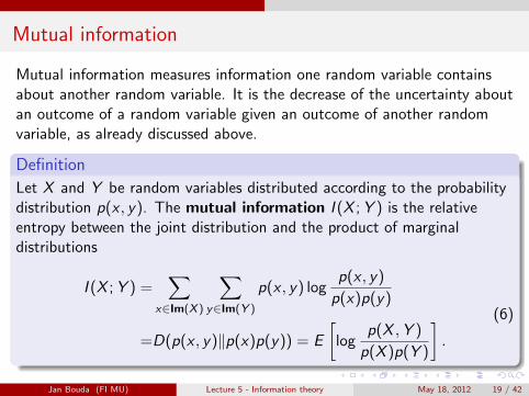
Mutual information

Mutual information measures information one random variable containsabout another random variable. It is the decrease of the uncertainty aboutan outcome of a random variable given an outcome of another randomvariable, as already discussed above.

Definition

Let X and Y be random variables distributed according to the probabilitydistribution p(x , y). The mutual information I (X ; Y ) is the relativeentropy between the joint distribution and the product of marginaldistributions

I (X ; Y ) =∑

x∈Im(X )

∑y∈Im(Y )

p(x , y) logp(x , y)

p(x)p(y)

=D(p(x , y)‖p(x)p(y)) = E

[log

p(X ,Y )

p(X )p(Y )

].

(6)


Mutual Information and Entropy

Theorem

I (X ; Y ) = H(X )− H(X |Y ).

Proof.

I (X ; Y ) =∑x ,y


p(x)p(y)==

∑x ,y

p(x , y) logp(x |y)

p(x)=

=−∑x ,y

p(x , y) log p(x) +∑x ,y


=−∑x ,y

p(x) log p(x)−

(−∑x ,y

p(x , y) log p(x |y)

)=

=H(X )− H(X |Y ).

(7)


Mutual information

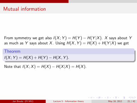
From symmetry we get also I (X ; Y ) = H(Y )− H(Y |X ). X says about Yas much as Y says about X . Using H(X ,Y ) = H(X ) + H(Y |X ) we get

Theorem

I (X ; Y ) = H(X ) + H(Y )− H(X ,Y ).

Note that I (X ; X ) = H(X )− H(X |X ) = H(X ).


Part IV

Properties of Entropy and Mutual Information


General Chain Rule for Entropy

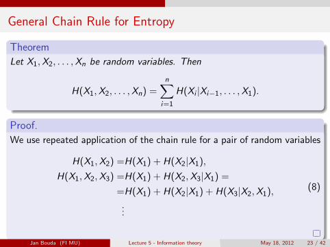
Theorem

Let X1,X2, . . . ,Xn be random variables. Then

H(X1,X2, . . . ,Xn) =n∑

i=1

H(Xi |Xi−1, . . . ,X1).

Proof.

We use repeated application of the chain rule for a pair of random variables

H(X1,X2) =H(X1) + H(X2|X1),

H(X1,X2,X3) =H(X1) + H(X2,X3|X1) =

=H(X1) + H(X2|X1) + H(X3|X2,X1),

...

(8)


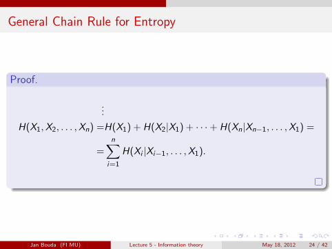
General Chain Rule for Entropy

Proof.

...

H(X1,X2, . . . ,Xn) =H(X1) + H(X2|X1) + · · ·+ H(Xn|Xn−1, . . . ,X1) =

=n∑

i=1

H(Xi |Xi−1, . . . ,X1).


Conditional Mutual Information

Definition

The conditional mutual information between random variables X and Ygiven Z is defined as

I (X ; Y |Z ) = H(X |Z )− H(X |Y ,Z ) = E

[log

p(X ,Y |Z )

p(X |Z )p(Y |Z )

],

where the expectation is taken over p(x , y , z).

Theorem (Chain rule for mutual information)

I (X1,X2, . . . ,Xn; Y ) =∑n

i=1 I (Xi ; Y |Xi−1, . . . ,X1)


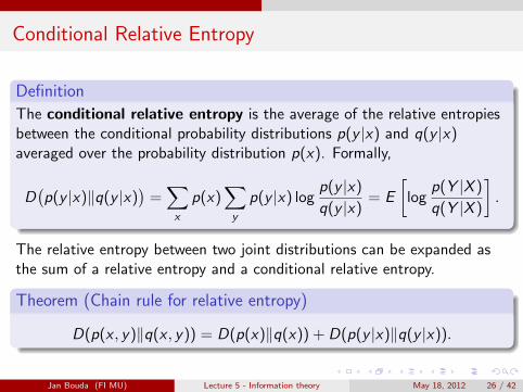
Conditional Relative Entropy

Definition

The conditional relative entropy is the average of the relative entropiesbetween the conditional probability distributions p(y |x) and q(y |x)averaged over the probability distribution p(x). Formally,

D(p(y |x)‖q(y |x)

)=∑x

p(x)∑y

p(y |x) logp(y |x)

q(y |x)= E

[log

p(Y |X )

q(Y |X )

].

The relative entropy between two joint distributions can be expanded asthe sum of a relative entropy and a conditional relative entropy.

Theorem (Chain rule for relative entropy)

D(p(x , y)‖q(x , y)) = D(p(x)‖q(x)) + D(p(y |x)‖q(y |x)).


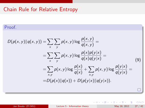
Chain Rule for Relative Entropy

Proof.

D(p(x , y)‖q(x , y)) =∑x

∑y


q(x , y)=

=∑x

∑y

p(x , y) logp(x)p(y |x)

q(x)q(y |x)=

=∑x ,y

p(x , y) logp(x)

q(x)+∑x ,y

p(x , y) logp(y |x)

q(y |x)=

=D(p(x)‖q(x)) + D(p(y |x)‖q(y |x)).

(9)


Part V

Information inequality


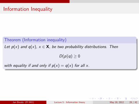
Information Inequality

Theorem (Information inequality)

Let p(x) and q(x), x ∈ X, be two probability distributions. Then

D(p‖q) ≥ 0

with equality if and only if p(x) = q(x) for all x.



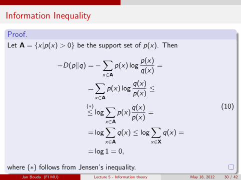
Proof.

Let A = {x |p(x) > 0} be the support set of p(x). Then

−D(p‖q) =−∑x∈A

p(x) logp(x)

q(x)=

=∑x∈A

p(x) logq(x)

p(x)≤

(∗)≤ log

∑x∈A

p(x)q(x)

p(x)=

= log∑x∈A

q(x) ≤ log∑x∈X

q(x) =

= log 1 = 0,

(10)

where (∗) follows from Jensen’s inequality.Jan Bouda (FI MU) Lecture 5 - Information theory May 18, 2012 30 / 42


Proof.

Since log t is a strictly concave function (implying − log t is strictly convex)of t, we have equality in (∗) if and only if q(x)/p(x) = 1 everywhere, i.e.p(x) = q(x). Also, if p(x) = q(x) the second inequality also becomesequality.

Corollary (Nonnegativity of mutual information)

For any two random variables X , Y

I (X ; Y ) ≥ 0

with equality if and only if X and Y are independent.

Proof.

I (X ; Y ) = D(p(x , y)‖p(x)p(y)) ≥ 0 with equality if and only ifp(x , y) = p(x)p(y), i.e. X and Y are independent.


Consequences of Information Inequality

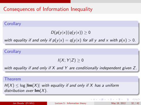
Corollary

D(p(y |x)‖q(y |x)) ≥ 0

with equality if and only if p(y |x) = q(y |x) for all y and x with p(x) > 0.

Corollary

I (X ; Y |Z ) ≥ 0

with equality if and only if X and Y are conditionally independent given Z.

Theorem

H(X ) ≤ log |Im(X )| with equality if and only if X has a uniformdistribution over Im(X ).



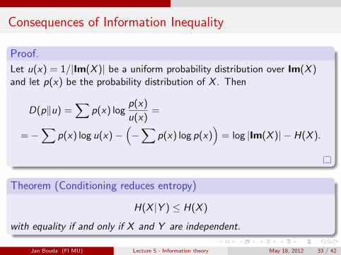
Proof.

Let u(x) = 1/|Im(X )| be a uniform probability distribution over Im(X )and let p(x) be the probability distribution of X . Then

D(p‖u) =∑

p(x) logp(x)

u(x)=

=−∑

p(x) log u(x)−(−∑

p(x) log p(x))

= log |Im(X )| − H(X ).

Theorem (Conditioning reduces entropy)

H(X |Y ) ≤ H(X )

with equality if and only if X and Y are independent.



Proof.

0 ≤ I (X ; Y ) = H(X )− H(X |Y ).

Previous theorem says that on average knowledge of a random variable Yreduces our uncertainty about other random variable X . However, theremay exist y such that H(X |Y = y) > H(X ).

Theorem (Independence bound on entropy)

Let X1,X2, . . . ,Xn be drawn according to p(x1, x2, . . . , xn). Then

H(X1,X2, . . . ,Xn) ≤n∑

i=1

H(Xi )

with equality if and only if Xi ’s are mutually independent.



Proof.

We use the chain rule for entropy

H(X1,X2, . . . ,Xn) =n∑

i=1

H(Xi |Xi−1, . . . ,X1)

≤n∑

i=1

H(Xi ),

(11)

where the inequality follows directly from the previous theorem. We haveequality if and only if Xi is independent of all Xi−1, . . . ,X1.


Part VI

Log Sum Inequality and Its Applications


Log Sum Inequality

Theorem (Log sum inequality)

For a nonnegative numbers a1, a2, . . . , an and b1, b2, . . . , bn it holds that

n∑i=1

ai logaibi≥

(n∑

i=1

ai

)log

∑ni=1 ai∑ni=1 bi

with equality if and only if ai/bi = const.

In the theorem we used again the convention that 0 log 0 = 0,a log(a/0) =∞ if a > 0 and 0 log(0/0) = 0.


Log Sum Inequality

Proof.

Assume WLOG that ai > 0 and bi > 0. The function f (t) = t log t isstrictly convex since f ′′(t) = 1

t log e > 0 for all positive t. We use theJensen’s inequality to get

∑i

αi f (ti ) ≥ f

(∑i

αi ti

)

for αi ≥ 0,∑

i αi = 1. Setting αi = bi/∑n

j=1 bj and ti = ai/bi we obtain

∑i

ai∑j bj

logaibi≥

(∑i

ai∑j bj

)log∑i

ai∑j bj

,

what is the desired result.


Consequences of Log Sum Inequality

Theorem

D(p‖q) is convex in the pair (p, q), i.e. if (p1, q1) and (p2, q2) are twopairs of probability distributions, then

D(λp1 + (1− λ)p2‖λq1 + (1− λ)q2) ≤ λD(p1‖q1) + (1− λ)D(p2‖q2)

for all 0 ≤ λ ≤ 1.

Theorem (Concavity of entropy)

H(p) is a concave function of p

Theorem

Let (X ,Y ) ∼ p(x , y) = p(x)p(y |x). The mutual information I (X ; Y ) is aconcave function of p(x) for fixed p(y |x) and a convex function of p(y |x)for fixed p(x).


Part VII

Data Processing inequality


Data Processing Inequality

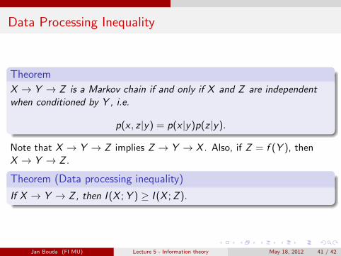
Theorem

X → Y → Z is a Markov chain if and only if X and Z are independentwhen conditioned by Y , i.e.

p(x , z |y) = p(x |y)p(z |y).

Note that X → Y → Z implies Z → Y → X . Also, if Z = f (Y ), thenX → Y → Z .

Theorem (Data processing inequality)

If X → Y → Z , then I (X ; Y ) ≥ I (X ; Z ).


Data Processing Inequality

Proof.

We expand mutual information using the chain rule in two different ways as

I (X ; Y ,Z ) =I (X ; Z ) + I (X ; Y |Z )

=I (X ; Y ) + I (X ; Z |Y ).(12)

Since X and Z are conditionally independent given Y we haveI (X ; Z |Y ) = 0. Since I (X ; Y |Z ) ≥ 0 we have

I (X ; Y ) ≥ I (X ; Z ).


lecture 5 - information theory - masaryk university · jan bouda (fi mu) lecture 5 - information...

Documents