lecture 5 models and methods for recurrent event data
TRANSCRIPT

Time-to-events models Time-between-events models
Lecture 5 Models and methods for recurrent event
dataRecurrent and multiple events are commonly encountered in longitudinal
studies. In this chapter we consider ordered recurrent and multiple events.
I Recurrent events (focused topic)
- time-to-events model (point process model)
- time-between-events model (gap times model)
- e.g. repeated infections/hospitalizations/tumor occurrences
I Ordered multiple events
- HIV → AIDS → death
- birth → onset age of a genetic disease → death
- disease staging I → II → III → IV
I Unordered multiple events
Time-to-events models Time-between-events models
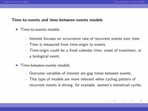
Time-to-events and time-between-events models
I Time-to-events models
- Interest focuses on occurrence rate of recurrent events over time.
- Time is measured from time-origin to events.
- Time-origin could be a fixed calendar time, onset of treatment, or
a biological event.
I Time-between-events models
- Outcome variables of interest are gap times between events.
- This type of models are more relevant when cycling pattern of
recurrent events is strong; for example, women’s menstrual cycles.
Time-to-events models Time-between-events models
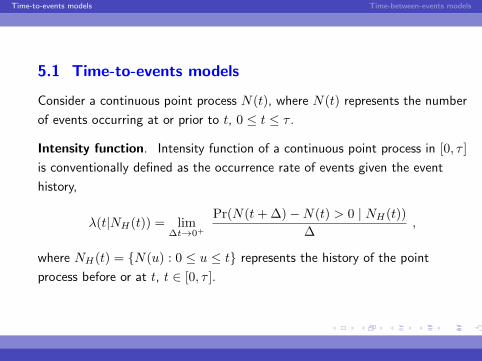
5.1 Time-to-events models
Consider a continuous point process N(t), where N(t) represents the number
of events occurring at or prior to t, 0 ≤ t ≤ τ .
Intensity function. Intensity function of a continuous point process in [0, τ ]
is conventionally defined as the occurrence rate of events given the event
history,
λ(t|NH(t)) = lim∆t→0+
Pr(N(t+ ∆)−N(t) > 0 | NH(t))
∆,
where NH(t) = {N(u) : 0 ≤ u ≤ t} represents the history of the point
process before or at t, t ∈ [0, τ ].
Time-to-events models Time-between-events models
Remarks
- The intensity function uniquely determines the probability structure of
the point process under regularity conditions.
- For recurrent events, the so-called conditional regression models are
constructed on the basis of the intensity function.
Time-to-events models Time-between-events models
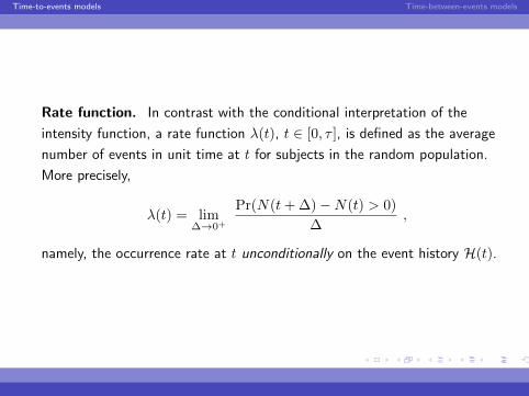
Rate function. In contrast with the conditional interpretation of the
intensity function, a rate function λ(t), t ∈ [0, τ ], is defined as the average
number of events in unit time at t for subjects in the random population.
More precisely,
λ(t) = lim∆→0+
Pr(N(t+ ∆)−N(t) > 0)
∆,
namely, the occurrence rate at t unconditionally on the event history H(t).
Time-to-events models Time-between-events models
Remarks
- In general, a rate function itself does not fully determine the probability
structure of the point process.
- The rate function is conceptually and quantitatively different from the
intensity function, and it coincide with the intensity function only when
the process is memoryless.
- For recurrent events, the so-called marginal regression models are
constructed on the basis of the rate function
Time-to-events models Time-between-events models
Define the cumulative rate function as
Λ(t) =
∫ t
0
λ(u)du , t ∈ [0, T0].
The CRF Λ(t) is also expectation of the number of recurrent events
occurring in [0, t]. Note that
E[N(t)] = Λ(t)
we frequently write
E[dN(t)] = λ(t)dt

Time-to-events models Time-between-events models
5.1.1 Poisson process models
Poisson process is a counting process model for multiple events occurring
over a fixed time interval [0, τ ], τ > 0. The Poisson distribution is the
probability distribution for the total number of events, M .
The Poisson distribution is sometimes used for modelling a count variable in
other situations.

Time-to-events models Time-between-events models
A point process is a stationary Poisson process if the following three
conditions are satisfied (sketch):
1. The probability that exactly one event occurs in a small interval
[t, t+ h] is approximately λh, where λ is called the intensity (or rate) of
events, λ > 0.
2. The probability that 2 or more events occur at the same time is
approximately 0.
3. The numbers of events in disjoint regions are independent.
Let µ = λτ > 0. The pdf of M is fM (m) =(
e−µµm
m!
), m = 0, 1, 2, . . ..
A Poisson process is called a non-stationary Poisson process if the
occurrence rate, λ(t), is time dependent.
Time-to-events models Time-between-events models
5.1.2 Nonparametric estimation of CRF
I Data. Let ti1 ≤ · · · ≤ ti,mi be the ordered event times with mi
defined as the index for the last observed event. The observed data
include {(mi, ci, ti1, . . . , ti,mi) : i = 1, . . . , n}.
I Population. Note that for a single event process (univariate survival
time), the risk population at t is composed of subjects who have not
failed prior to t, thus the risk population varies with different values of t.
In contrast, for a recurrent event process, the risk population at
different t’s always coincides with the target population defined at 0.
I Risk set. Let Ci represent the terminating time (censoring time) for
observing N(t). The risk set at t is defined as {i : Ci ≥ t} which
includes subjects who are under observation at t. Define
Ri(t) = I(Ci > t) as the risk-set indicator, and R(t) =∑ni=1Ri(t).
I Independent censoring. If Ci is independent of Ni(·) , the risk set
forms a random sample from the risk population at t.
Time-to-events models Time-between-events models
Under independent censoring assumption, for t > 0 and positive-valued but
small ∆, a crude estimate of the occurrence probability in (t−∆, t] can
constructed as
λ(t)∆ ≈∑ni=1
∑mij=1 I(tij ∈ (t−∆, t])
R(t), (1)
with I(·) representing the indicator function. The estimate is essentially an
empirical measure with time-dependent sample size R(t). A nonparametric
estimate of the CRF corresponding to (1) can then be constructed as
Λ(t) =
n∑i=1
mi∑j=1
I(tij ≤ t)R(tij)
. (2)
Nelson (88, JQT; 95, Technometrics)

Time-to-events models Time-between-events models
5.1.3 Conditional Regression Models
Anderson and Gill (1982, AS) proposed a time-to-events model which
extended Cox’s proportional hazards model from single event data to
recurrent event data. Suppose the dates of recurrent events are recorded with
a continuous scale (e.g., by days or weeks), and the outcome measures of
interest are recurrent events occurring in the time interval [0, τ ], where the
constant τ > 0 is determined with the knowledge that recurrent events could
potentially be observed up to τ , say 3 years.
I Let NH(t) be the recurrent event history and ZH(t) the possibly
time-dependent covariate history prior to t.
I For t ∈ [0, τ ], the AG model assumes the events occur over time with
the occurrence rate
λ(t | NH(t), ZH(t)) = λ0(t)exp{X(t)β}, (3)
where X(t) = φ(NH(t), ZH(t)) is a transformation of (NH(t), ZH(t))
Time-to-events models Time-between-events models
Pros and cons of conditional regression model
(i) The AG model can be thought of as a predicting model since the event
history is included as a part of conditional statistics in the rate function.
(ii) Use of the AG model to identify treatment effects is subject to
constraints, since the model identifies treatment effects adjusted for
subject-specific event history. In general, AG model is not ideal for
identifying treatment effects or population risks.
(iii) If the AG model chooses to use time-independent covariate, X(t) = X,
the model is then required to be memoryless. For example, two subjects
with the same X but different event histories would predict the same
occurrence rate of events. Thus, if X =treatment indicator, two
patients who receive the same treatment but have different
hospitalization records would have the same level of risk for
rehospitalization according to the AG model.
Time-to-events models Time-between-events models
Statistical methods for conditional regression model
AG extended the partial likelihood methods from univariate survival data to
recurrent event data.
The partial likelihood score function for β0 can be derived as
U(β, t) =
n∑i=1
∫ t
0
{Xi(u)− X(β, u)}dNi(u) (4)
where Z(β, t) =∑ni=1 Ri(t)Xi(t) exp{βT0 Xi(t)}∑n
i=1 Ri(t) exp{βT0 Xi(t)}. Martingale theory was also
developed to establish the large sample properties (as an extension of
martingale theory for univariate survival analysis).
Time-to-events models Time-between-events models
5.1.4 Marginal Regression Models
In stead of the conditional regression model, we may consider a marginal
model where the event history, N(t), is not included as part of the
conditional statistics:
λ(t | Z(t)) = λ0(t)exp{Z(t)β} .
The marginal model is generally ideal for identifying treatment effects and
risk factors, but the estimation procedure of LWYY depends heavily on the
independent censoring assumption. The LWYY estimates could be very
biased when the follow-up is terminated by reasons associated with the
recurrent events such as informative drop-out or death. Statistical inferences
can be found in the articles of Pepe and Cai (1993, JASA) and Lin et al.
(Huang, 2000, JRSS-B).
Time-to-events models Time-between-events models
5.1.5 Semi-parametric latent variable models.
With intension to deal with censoring due to death or informative drop-out,
Wang et al. (2001, JASA) proposed a semi-parametric latent variable model
for time-to-events data:
λ(t | Z,X) = Z · λ0(t)exp{Xβ}
The model allows for informative censoring through the use of a latent
variable. The model implies the marginal rate model
λ(t | X = x) = λ∗0(t)exp{xβ}. where λ∗0(t) = E[Z] · λ0(t). The model has
the feature of treating both the censoring and latent variable distributions as
nonparametric components. The approach avoids modeling and estimating
these nonparametric components by proper conditional likelihood techniques.
As a related work, a joint model for recurrent events and a failure time was
proposed and studied by Huang and Wang (2004, JASA).
Time-to-events models Time-between-events models
5.2 Time-between-events models
Suppose the outcome measure of interest is time between successive events
(gap time). When time-between-events is the variable of interest, the
occurrence of each recurrent event is considered as the time origin for the
occurrence of the next event. Recurrence times could be considered as a type
of correlated failure time data in survival analysis. This type of correlated
data are, however, different from the correlated data collected from families
(e.g., twin data or sibling data) due to the ordering nature of recurrent
events.
Time-to-events models Time-between-events models
5.2.1 Specific features of data
Informative m. For typical multivariate survival data such as family data,
cluster size is usually assumed to be uncorrelated with failure times of a
cluster. For recurrence time data, the number of recurrent events, m, is
typically correlated with recurrence times in follow-up studies - large m is
likely to imply shorter times and vice versa. In some applications, m is even
used as the outcome measurement for analysis; e.g., in a Poisson model, m is
the Poisson count variable.
Induced informative censoring. Induced informative censoring is a special
feature for ordered events. When the observation of the recurrent event
process is censored at C, the censoring time for Tj is max{C −∑j−1k=1 Yk, 0},
for each j = 2, 3, . . .. Because∑j−1k=1 Yk is correlated with Tj for j ≥ 2,
recurrence times of order greater than one are observed subject to
informative censoring even if the censoring time C is independent of N(·).

Time-to-events models Time-between-events models
Intercepted sampling. The intercepted sampling is a well-known probability
feature of renewal processes. It is a specific feature of recurrence time data
because the sampling scheme to observe recurrence times in longitudinal
studies is similar to the intercepted sampling of renewal processes. For
simplicity of understanding, assume the recurrence times {Yj : j = 1, 2, . . .}are independent and identically distributed (iid). Let f , S and µ represent
the density function, survival function and mean of Yj . Let T = C − Tm and
R = Tm+1 − C be the so-called backward and forward recurrence times.
When the censoring time, C, is sufficiently large so that an equilibrium
condition is reached, the joint density of (T,R) can then be derived as
pT,R
(t, r) = f(t+ r)I(t ≥ 0, r ≥ 0)/µ . (5)
Time-to-events models Time-between-events models
The marginal density functions of Y , T and R can be derived, based on (1),
as
pYm+1
(y) = yf(y)I(y ≥ 0)/µ, (6)
pT
(t) = S(t)I(t ≥ 0)/µ, (7)
pR
(r) = S(r)I(r ≥ 0)/µ. (8)
The distribution of Ym+1 is referred to as the length-biased distribution. In
most of the longitudinal studies, however, the censoring time is not very large
and therefore the equilibrium condition is not satisfied. In these cases,
although the above distributional results do not hold, the bias from Ym+1 is
still significant and one should be careful when conducting statistical analysis.
In general, because of the specific data features, standard statistical methods
in survival analysis may or may not be appropriate for recurrence time data.
Time-to-events models Time-between-events models
5.2.2 Transitional probability Model
Let fj(y|yi1, . . . , yi,j−1) denote the pdf of Yij conditioning on
(Yi1, . . . , Yi,j−1) = (yi1, . . . , yi,j−1). Suppose the censoring time Ci is
independent of the recurrent event process Ni(·). Note that the likelihood
function is
L ∝n∏i=1
{mi∏j=1
fj(yij | yi1, . . . , yi,j−1)}Smi+1(y+i,mi+1 | yi1, . . . , yi,mi)
A“transitional probability model” can be constructed by placing distributional
assumptions on the conditional probability fj(y|yi1, . . . , yi,j−1). In
applications, when a transitional probability model is used, it is frequently
accompanied by a further 1st-order (or 2nd-order) markovian assumption that
the conditional pdf of Yij depends on (Yi1, . . . , Yi,j−1) only through Yi,j−1.
Time-to-events models Time-between-events models
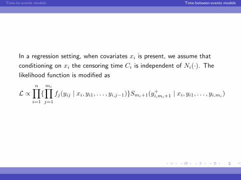
In a regression setting, when covariates xi is present, we assume that
conditioning on xi the censoring time Ci is independent of Ni(·). The
likelihood function is modified as
L ∝n∏i=1
{mi∏j=1
fj(yij | xi, yi1, . . . , yi,j−1)}Smi+1(y+i,mi+1 | xi, yi1, . . . , yi,mi)
Time-to-events models Time-between-events models
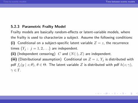
5.2.3 Parametric Frailty Model
Frailty models are basically random-effects or latent-variable models, where
the frailty is used to characterize a subject. Assume the following conditions:
(i) Conditional on a subject-specific latent variable Z = z, the recurrence
times {Yj : j = 1, 2, . . .} are independent.
(ii) (Independent censoring) C and (N(·), Z) are independent.
(iii) (Distributional assumption) Conditional on Z = z, Yj is distributed with
pdf fj(y | z; θ), θ ∈ Θ. The latent variable Z is distributed with pdf h(z; γ),
γ ∈ Γ.
Time-to-events models Time-between-events models
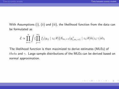
With Assumptions (i), (ii) and (iii), the likelihood function from the data can
be formulated as
L ∝n∏i=1
∫{mi∏j=1
fj(yij | zi; θ)}Smi+1(y+i,mi+1 | zi; θ)h(zi; γ)dzi
The likelihood function is then maximized to derive estimates (MLEs) of
theta and γ. Large sample distributions of the MLEs can be derived based on
normal approximation.
Time-to-events models Time-between-events models
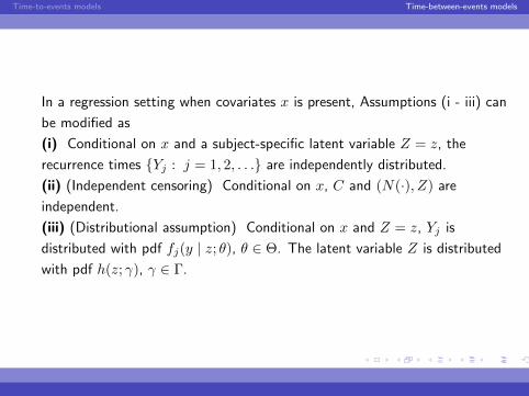
In a regression setting when covariates x is present, Assumptions (i - iii) can
be modified as
(i) Conditional on x and a subject-specific latent variable Z = z, the
recurrence times {Yj : j = 1, 2, . . .} are independently distributed.
(ii) (Independent censoring) Conditional on x, C and (N(·), Z) are
independent.
(iii) (Distributional assumption) Conditional on x and Z = z, Yj is
distributed with pdf fj(y | z; θ), θ ∈ Θ. The latent variable Z is distributed
with pdf h(z; γ), γ ∈ Γ.
Time-to-events models Time-between-events models
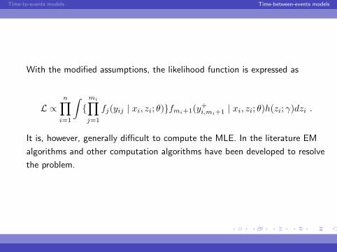
With the modified assumptions, the likelihood function is expressed as
L ∝n∏i=1
∫{mi∏j=1
fj(yij | xi, zi; θ)}fmi+1(y+i,mi+1 | xi, zi; θ)h(zi; γ)dzi .
It is, however, generally difficult to compute the MLE. In the literature EM
algorithms and other computation algorithms have been developed to resolve
the problem.

Time-to-events models Time-between-events models
Appendix (optional reading)
A.1 Nonparametric estimation of survival function estimation
Recurrence times can be treated as a type of correlated survival data in
statistical analysis. However, because of the ordinal nature of recurrence
times, statistical methods which are appropriate for clustered survival data
may not be applicable to recurrence time data. In many medical papers,
recurrence time data are frequently analyzed by inappropriate methods as
indicated by Aalen and Husebye (1991). Specifically, for estimating the
marginal survival function, the Kaplan-Meier estimator derived from the
pooled data is frequently used for exploratory analysis although the estimator
is generally inappropriate for such analyses. Suppose recurrent events are of
the same type and consider the problem of how to estimate the marginal
survival function from univariate recurrence time data. Assume the following
conditions are satisfied.
Time-to-events models Time-between-events models
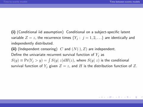
(i) (Conditional iid assumption) Conditional on a subject-specific latent
variable Z = z, the recurrence times {Yj : j = 1, 2, . . .} are identically and
independently distributed.
(ii) (Independent censoring) C and (N(·), Z) are independent.
Define the univariate recurrent survival function of Yj as
S(y) ≡ Pr(Yj > y) =∫S(y| z)dH(z), where S(y| z) is the conditional
survival function of Yj given Z = z, and H is the distribution function of Z.

Time-to-events models Time-between-events models
Under (i) and (ii), let S = 1− S, the nonparametric likelihood function can
be formulated as
n∏i=1
∫[
mi∏j=1
dS(uij |zi)]S(u+i,mi+1|zi)dH(zi) .
Conceptually, the likelihood function involves both infinite parameters (the
conditional cdf’s S(·|zi)) and a mixing distribution (H). With infinite
parameters, the maximization of the likelihood function could be problematic
and therefore it is not used as the tool for finding an estimator of S. Instead
of the nonparametric likelihood approach, Wang and Chang (1999, JASA)
proposed a class of nonparametric estimators for estimating S(y):
Time-to-events models Time-between-events models
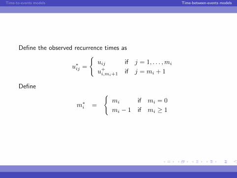
Define the observed recurrence times as
u∗ij =
{uij if j = 1, . . . ,mi
u+i,mi+1 if j = mi + 1
Define
m∗i =
{mi if mi = 0
mi − 1 if mi ≥ 1
Time-to-events models Time-between-events models
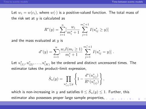
Let wi = w(ci), where w(·) is a positive-valued function. The total mass of
the risk set at y is calculated as
R∗(y) =
n∑i=1
[wi
m∗i + 1
m∗i+1∑j=1
I(u∗ij ≥ y)]
and the mass evaluated at y is
d∗(y) =
n∑i=1
[wiI(mi ≥ 1)
m∗i + 1
m∗i+1∑j=1
I(u∗ij = y)] .
Let u∗(1), u∗(2), . . . , u
∗(K) be the ordered and distinct uncensored times. The
estimator takes the product–limit expression,
Sn(y) =∏
u∗(i)≤y
{1−
d∗(u∗(i))
R∗(u∗(i))
},
which is non-increasing in y and satisfies 0 ≤ Sn(y) ≤ 1. Further, this
estimator also possesses proper large sample properties.
Time-to-events models Time-between-events models
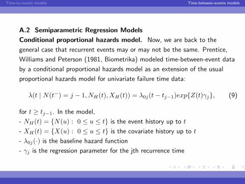
A.2 Semiparametric Regression Models
Conditional proportional hazards model. Now, we are back to the
general case that recurrent events may or may not be the same. Prentice,
Williams and Peterson (1981, Biometrika) modeled time-between-event data
by a conditional proportional hazards model as an extension of the usual
proportional hazards model for univariate failure time data:
λ(t | N(t−) = j − 1, NH(t), XH(t)) = λ0j(t− tj−1)exp{Z(t)γj}, (9)
for t ≥ tj−1. In the model,
- NH(t) = {N(u) : 0 ≤ u ≤ t} is the event history up to t
- XH(t) = {X(u) : 0 ≤ u ≤ t} is the covariate history up to t
- λ0j(·) is the baseline hazard function
- γj is the regression parameter for the jth recurrence time

Time-to-events models Time-between-events models
The possibly time-dependent covariate history up to t is denoted by XH(t).
As an important requirement, the event history NH(t) must be part of the
given knowledge (conditional statistics) in the PWP model. The
time-dependent covariate vector Z(t) = φ(XH(t), NH(t)) is a transformation
of (XH(t), NH(t)). This model serves as a proper model for predicting the
future events given subject-specific covariates and event history information.
However, since event history is part of the conditional statistics in the model,
the PWP model does not serve as an appropriate model for identifying
treatment or prevention effects. The PWP model has been further extended
to include both globally defined parameters β and episode-specific parameters
γj (Chang and Wang, 1999, JASA):
λ(t | N(t−) = j − 1, NH(t), XH(t)) = λ0j(t− tj−1)exp{Z(t)γj +W (t)β}, (10)
for t ≥ tj−1, where Z(t) and W (t) are functions of (XH(t), NH(t)).
Time-to-events models Time-between-events models
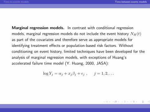
Marginal regression models. In contrast with conditional regression
models, marginal regression models do not include the event history NH(t)
as part of the covariates and therefore serve as appropriate models for
identifying treatment effects or population-based risk factors. Without
conditioning on event history, limited techniques have been developed for the
analysis of marginal regression models, with exceptions of Huang’s
accelerated failure time model (Y. Huang, 2000, JASA):
log Yj = αj + xjβj + εj , j = 1, 2, . . .
Time-to-events models Time-between-events models
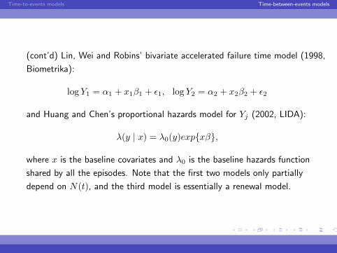
(cont’d) Lin, Wei and Robins’ bivariate accelerated failure time model (1998,
Biometrika):
log Y1 = α1 + x1β1 + ε1, log Y2 = α2 + x2β2 + ε2
and Huang and Chen’s proportional hazards model for Yj (2002, LIDA):
λ(y | x) = λ0(y)exp{xβ},
where x is the baseline covariates and λ0 is the baseline hazards function
shared by all the episodes. Note that the first two models only partially
depend on N(t), and the third model is essentially a renewal model.

Time-to-events models Time-between-events models
Trend models. In many applications the distributional pattern of
recurrence times can be used as an index for the progression of a disease.
Such a distributional pattern is important for understanding the natural
history of a disease or for confirming long-term treatment effect. Assume
(i) Within each subject, the recurrence times Y1, Y2, . . . are independently
distributed with the survival functions S0, S1, S2, . . ., and
(ii) within each subject, the censoring time C is independent of N(·).
Time-to-events models Time-between-events models
Assumption (i) can be viewed as a frailty condition where the conditional
independence of recurrence times holds within each subject. Assumption (ii)
implies that, within subject, the censoring mechanism is uninformative for the
probability structure of event process. In applications, one might be
interested in testing the null hypothesis (that is, (i)) that the duration
distributions of different episodes Y1, Y2, . . . remain the same to confirm the
stability of pattern of recurrence times, or to identify the treatment efficacy
over time; see Wang and Chen (2001, Biometrics) for nonparametric and
semiparametric approaches to deal with the problem.