lecture 5 - nn 2018-19 · chapter 6. deep feedforward networks y h x w w y h 1 x 1 h 2 x 2 figure...
TRANSCRIPT
Neural NetworksLecture 5: Back-propagation
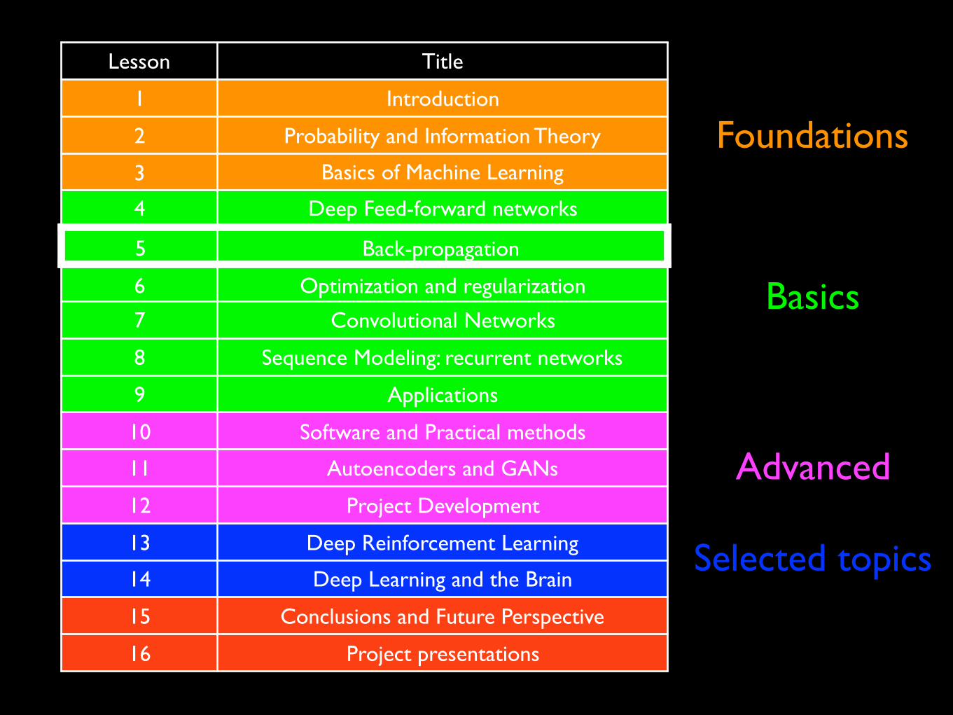
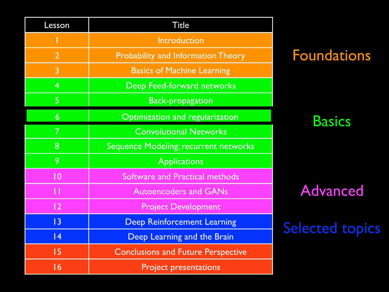
Selected topics
Advanced
Basics
Foundations
Lesson Title
1 Introduction
2 Probability and Information Theory
3 Basics of Machine Learning
4 Deep Feed-forward networks
5 Back-propagation
6 Optimization and regularization
7 Convolutional Networks
8 Sequence Modeling: recurrent networks
9 Applications
10 Software and Practical methods
11 Autoencoders and GANs
12 Project Development
13 Deep Reinforcement Learning
14 Deep Learning and the Brain
15 Conclusions and Future Perspective
16 Project presentations
CHAPTER 6. DEEP FEEDFORWARD NETWORKS
yy
hh
xx
W
w
yy
h1h1
x1x1
h2h2
x2x2
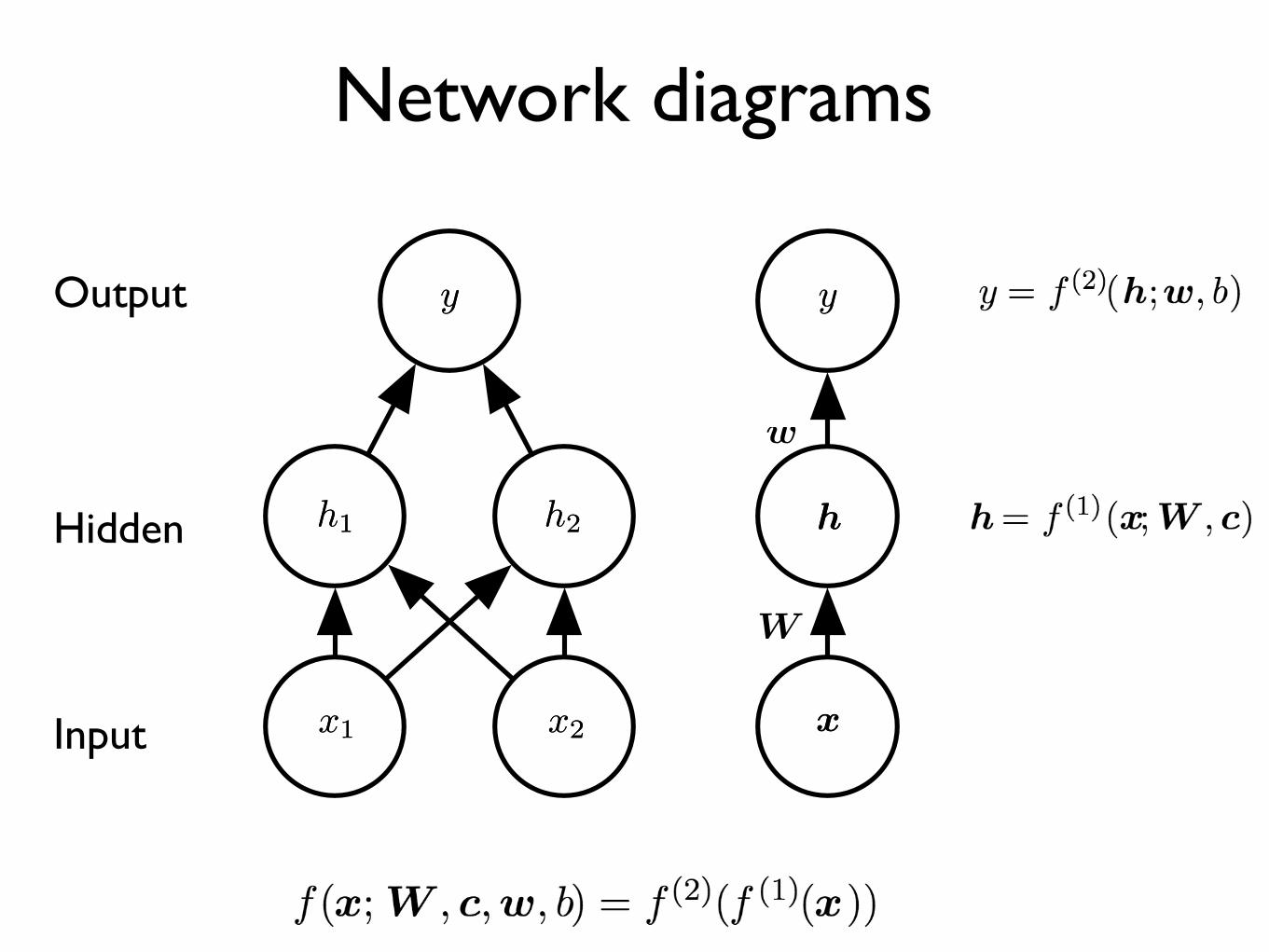
Figure 6.2: An example of a feedforward network, drawn in two different styles. Specifically,this is the feedforward network we use to solve the XOR example. It has a single hiddenlayer containing two units. (Left)In this style, we draw every unit as a node in the graph.This style is very explicit and unambiguous but for networks larger than this exampleit can consume too much space. (Right)In this style, we draw a node in the graph foreach entire vector representing a layer’s activations. This style is much more compact.Sometimes we annotate the edges in this graph with the name of the parameters thatdescribe the relationship between two layers. Here, we indicate that a matrix W describesthe mapping from x to h, and a vector w describes the mapping from h to y. Wetypically omit the intercept parameters associated with each layer when labeling this kindof drawing.
model, we used a vector of weights and a scalar bias parameter to describe anaffine transformation from an input vector to an output scalar. Now, we describean affine transformation from a vector x to a vector h, so an entire vector of biasparameters is needed. The activation function g is typically chosen to be a functionthat is applied element-wise, with hi = g(x>
W:,i + ci). In modern neural networks,the default recommendation is to use the rectified linear unit or ReLU (Jarrettet al., 2009; Nair and Hinton, 2010; Glorot et al., 2011a) defined by the activationfunction g(z) = max{0, z} depicted in figure 6.3.
We can now specify our complete network as
f(x; W , c, w, b) = w> max{0, W >
x + c} + b. (6.3)
We can now specify a solution to the XOR problem. Let
W =
1 11 1
�, (6.4)
c =
0
�1
�, (6.5)
174
Network diagrams
Input
Output
Hidden
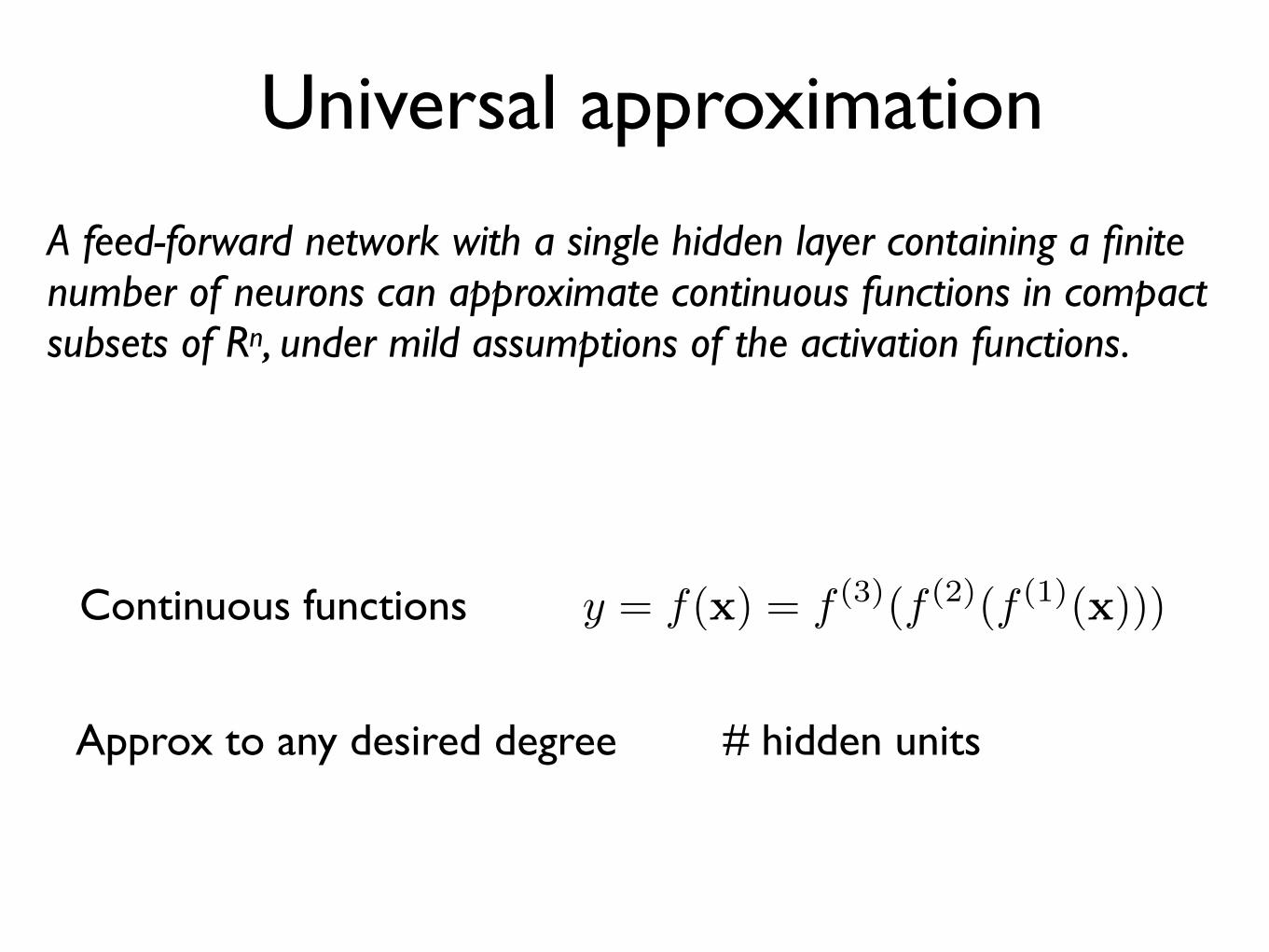
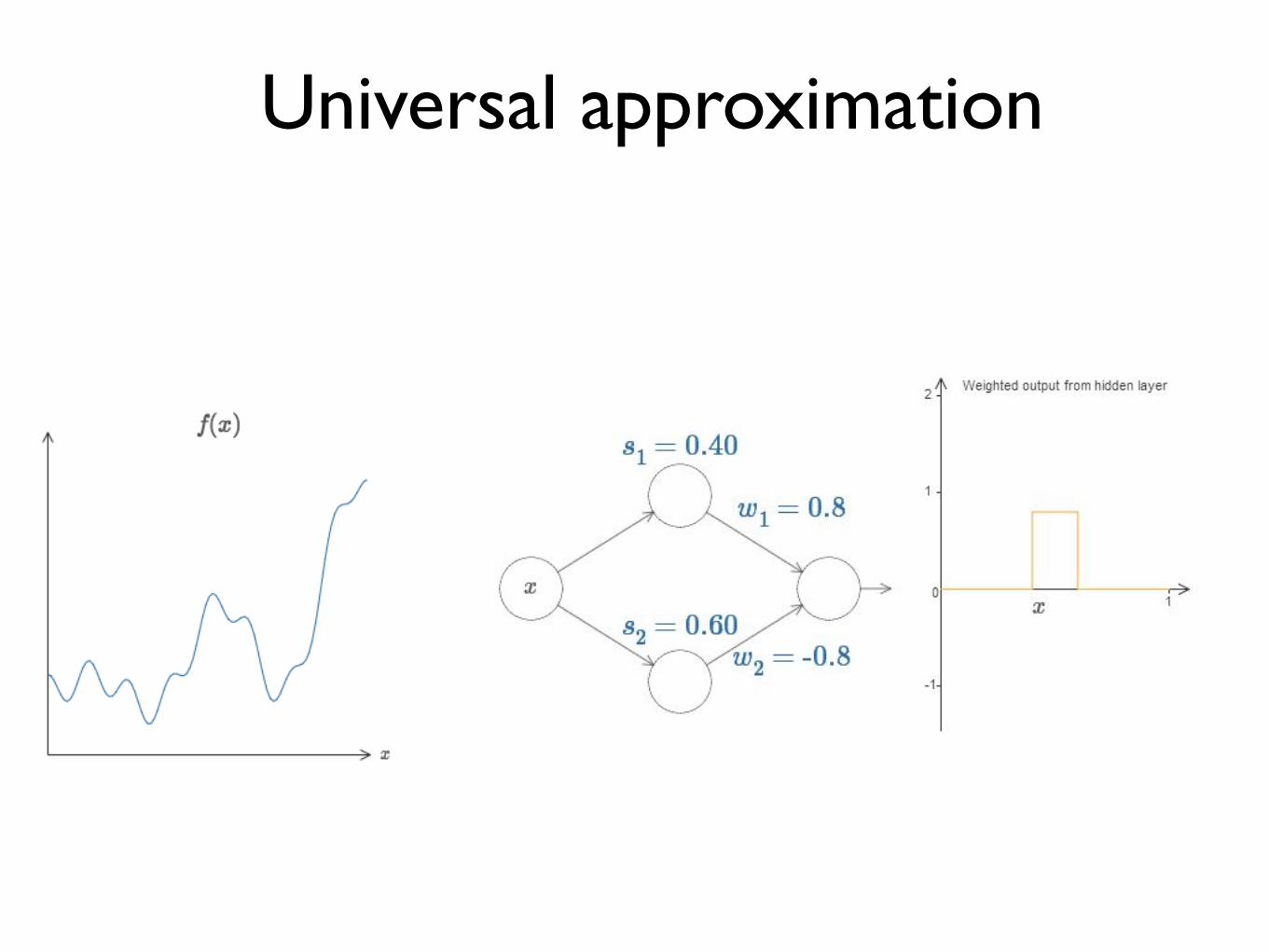
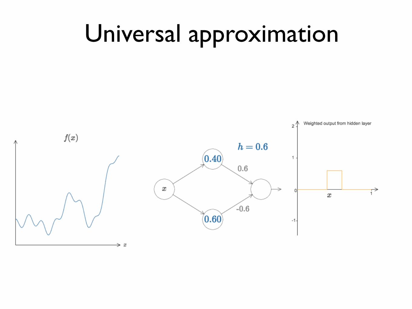
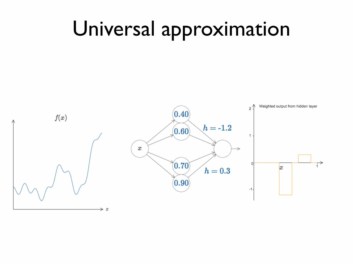
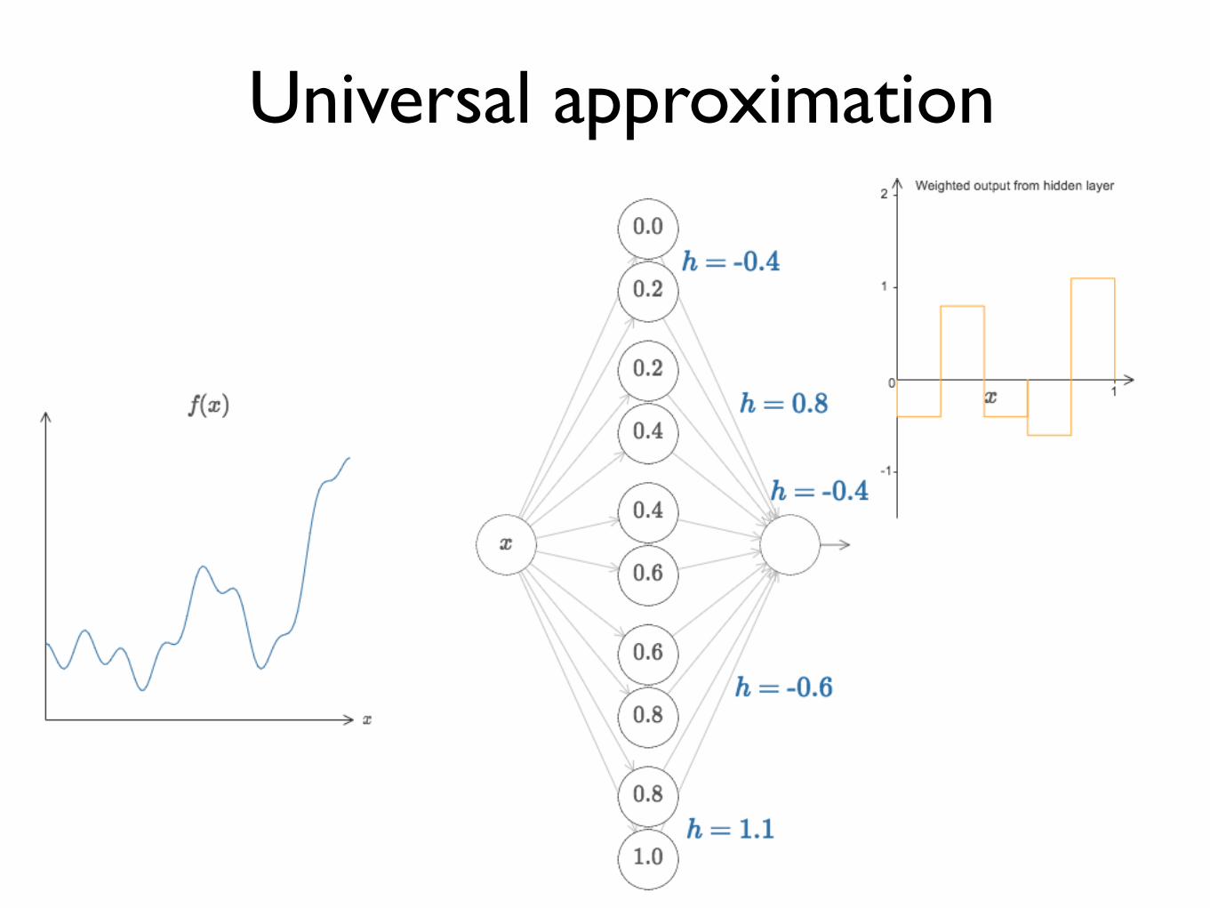
Universal approximation
Continuous functions
Approx to any desired degree
y = f(x) = f (3)(f (2)(f (1)(x)))
# hidden units
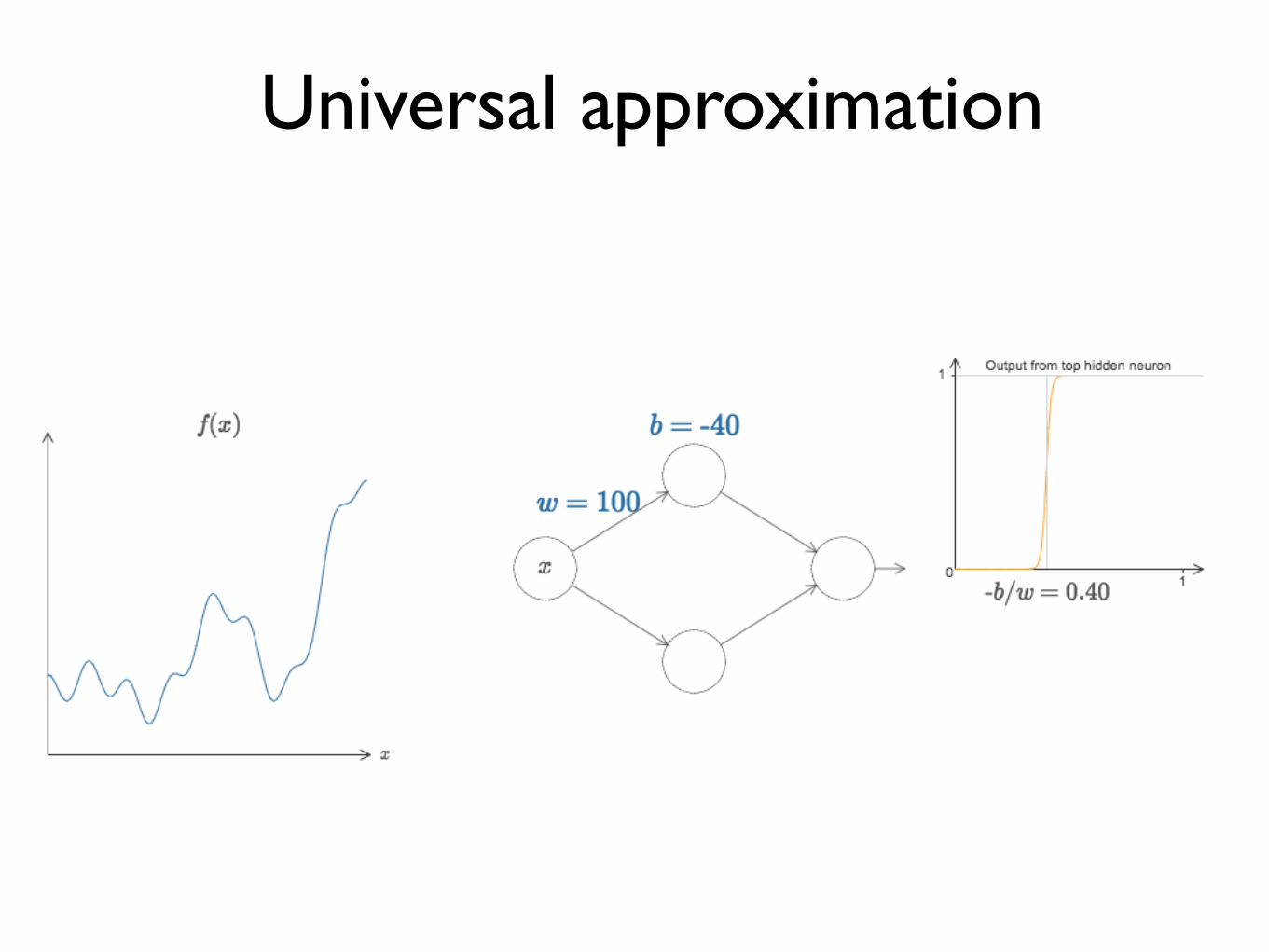
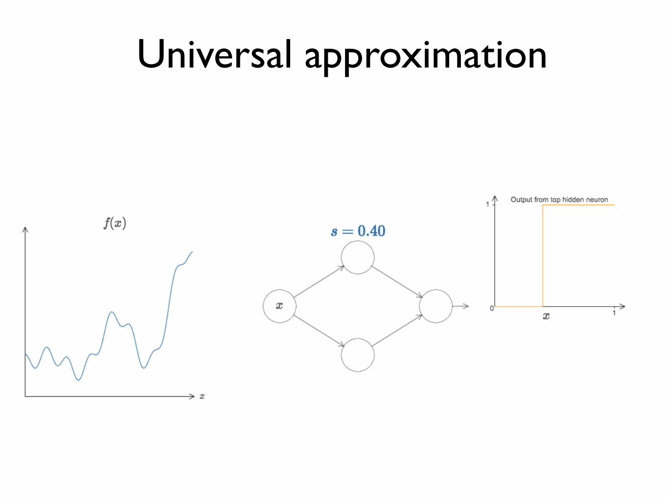
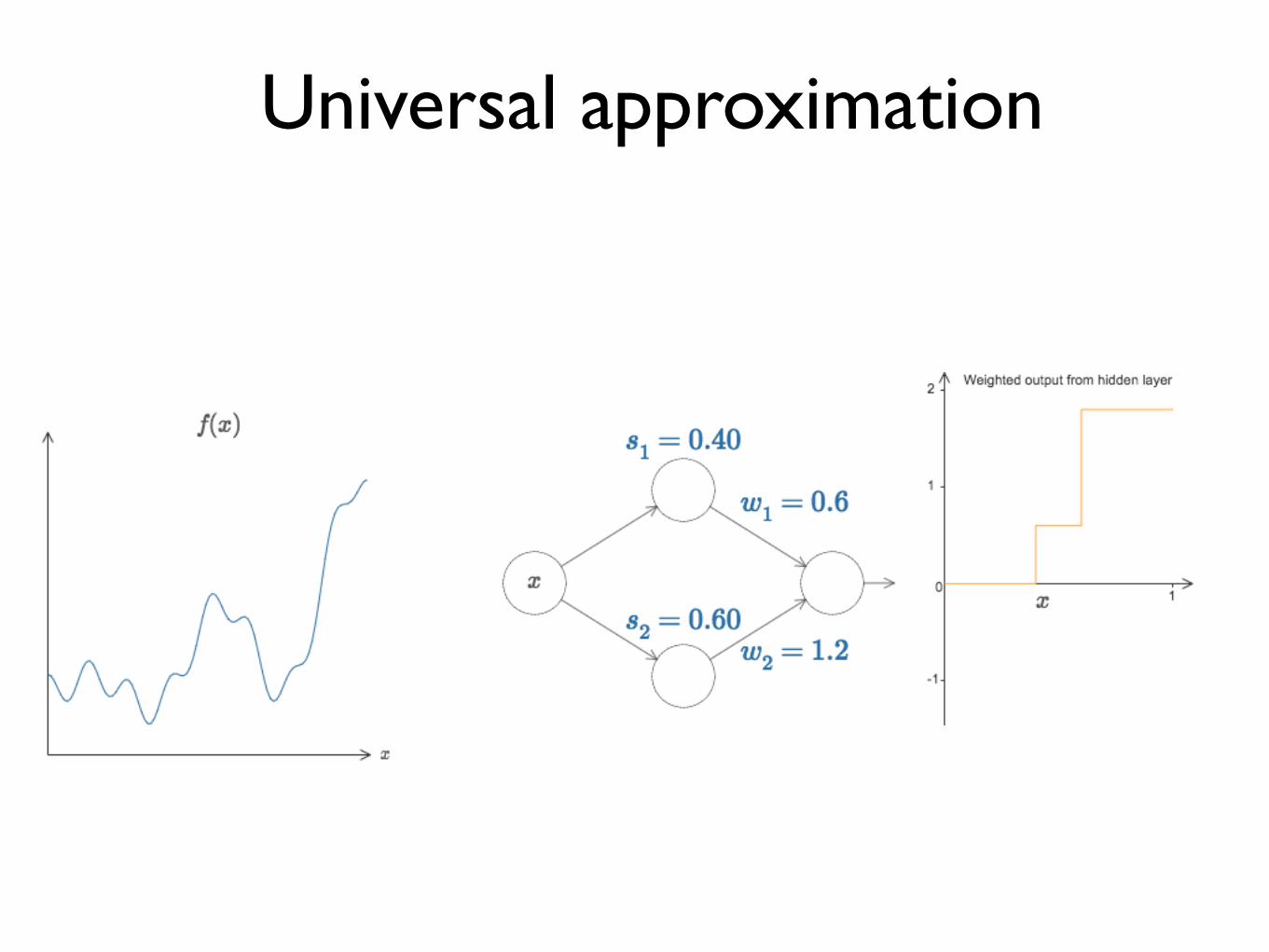
A feed-forward network with a single hidden layer containing a finite number of neurons can approximate continuous functions in compact subsets of Rn, under mild assumptions of the activation functions.
Universal approximation
Universal approximation
Universal approximation
Universal approximation
Universal approximation
Universal approximation
Universal approximation
(Goodfellow 2016)
Better Generalization with Greater DepthCHAPTER 6. DEEP FEEDFORWARD NETWORKS
3 4 5 6 7 8 9 10 11
Number of hidden layers
92.0
92.5
93.0
93.5
94.0
94.5
95.0
95.5
96.0
96.5
Tes
tacc
ura
cy(p
erce
nt)
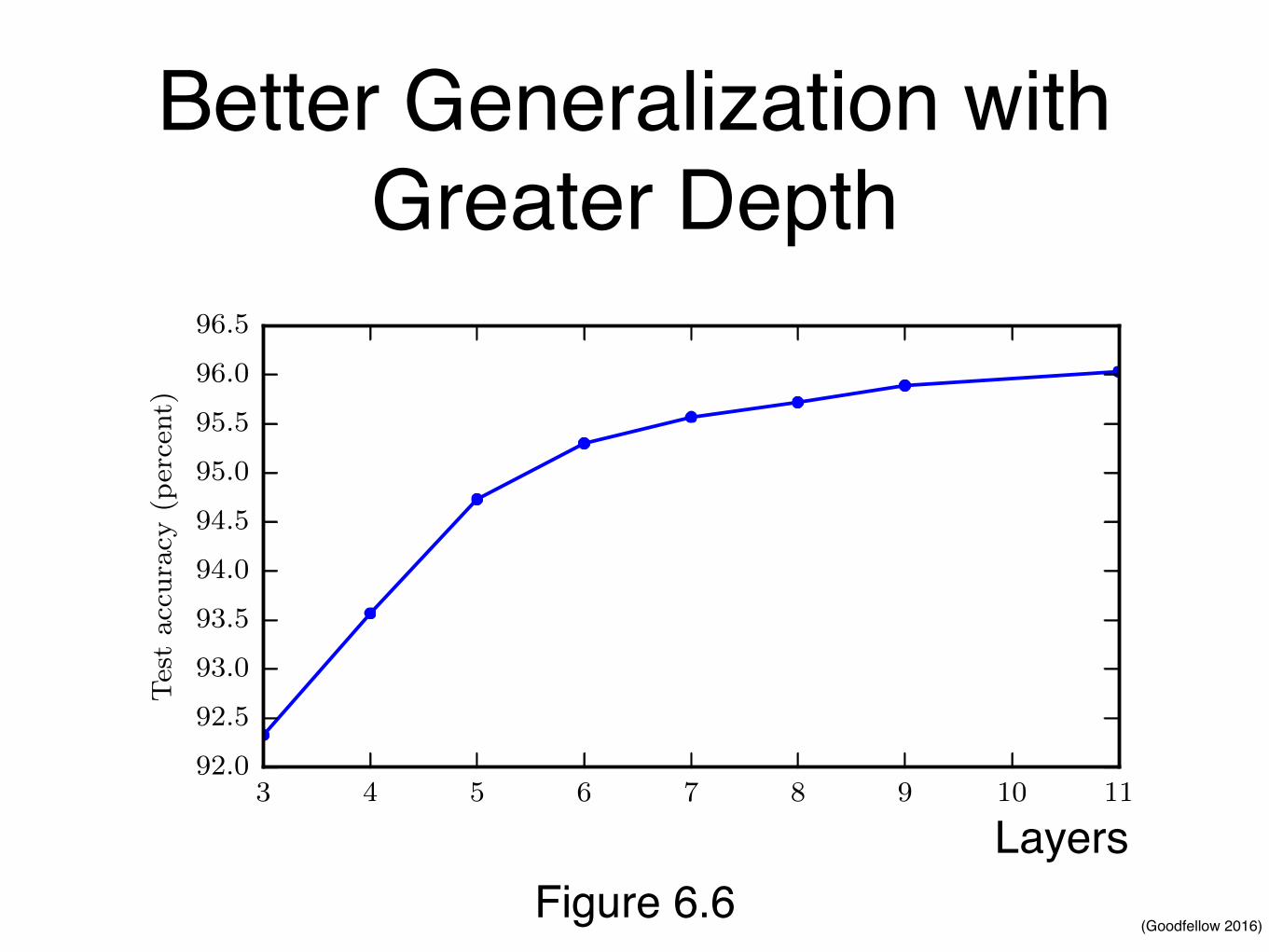
Figure 6.6: Empirical results showing that deeper networks generalize better when usedto transcribe multi-digit numbers from photographs of addresses. Data from Goodfellowet al. (2014d). The test set accuracy consistently increases with increasing depth. Seefigure 6.7 for a control experiment demonstrating that other increases to the model sizedo not yield the same effect.
Another key consideration of architecture design is exactly how to connect apair of layers to each other. In the default neural network layer described by a lineartransformation via a matrix W , every input unit is connected to every outputunit. Many specialized networks in the chapters ahead have fewer connections, sothat each unit in the input layer is connected to only a small subset of units inthe output layer. These strategies for reducing the number of connections reducethe number of parameters and the amount of computation required to evaluatethe network, but are often highly problem-dependent. For example, convolutionalnetworks, described in chapter 9, use specialized patterns of sparse connectionsthat are very effective for computer vision problems. In this chapter, it is difficultto give much more specific advice concerning the architecture of a generic neuralnetwork. Subsequent chapters develop the particular architectural strategies thathave been found to work well for different application domains.
202
Figure 6.6Layers
Learning objectives
• Understand the basics of gradient descent
• Apply back-propagation to estimate the gradients with respect to weights
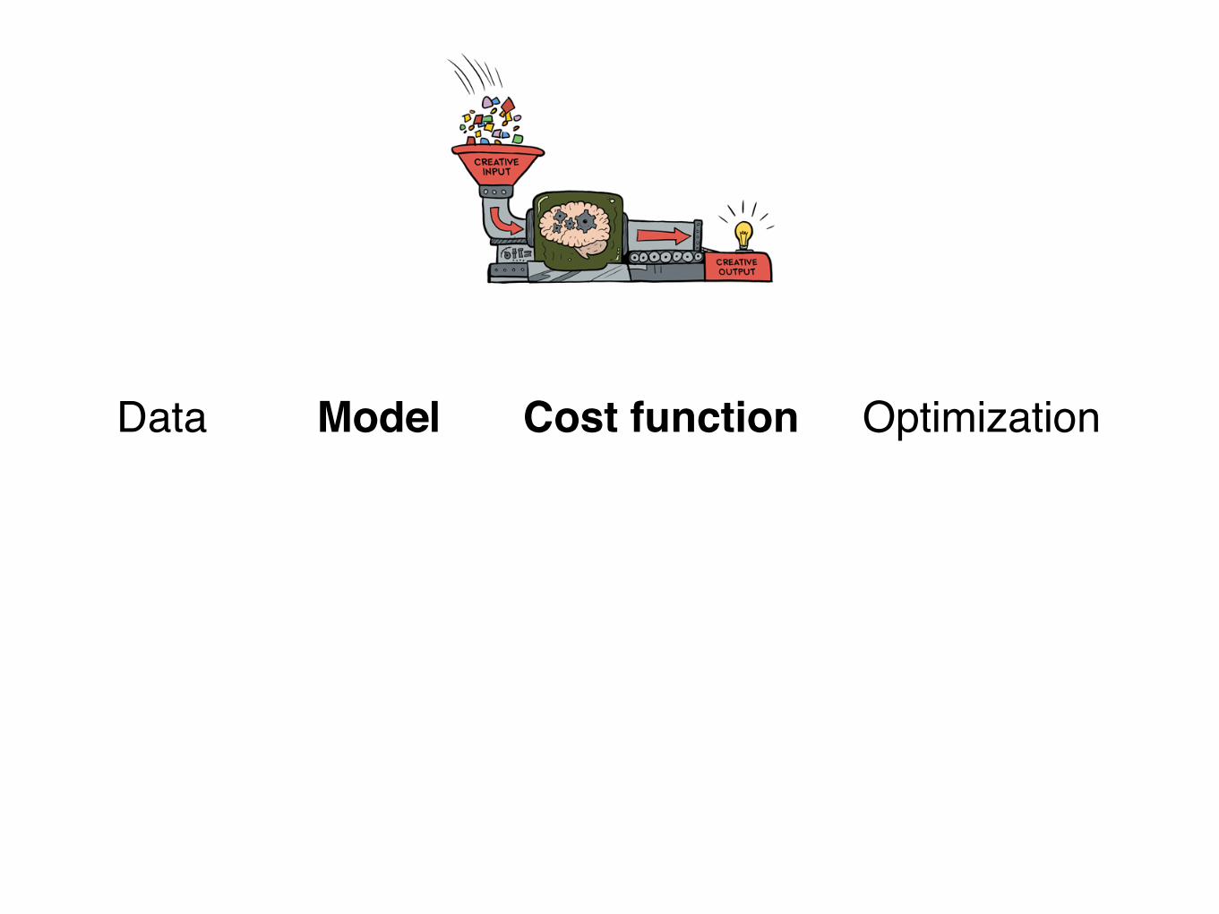
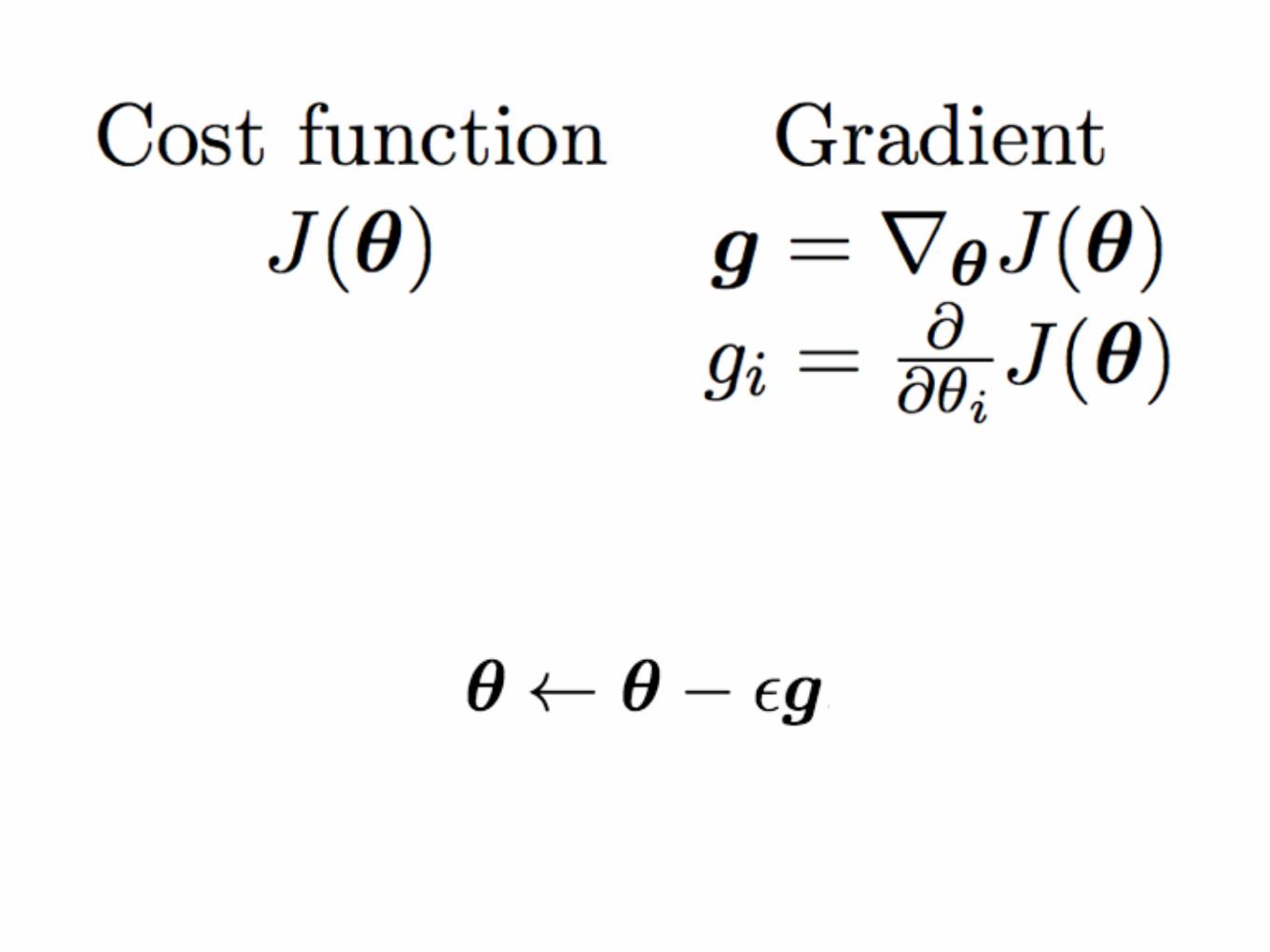
Data Model Cost function Optimization
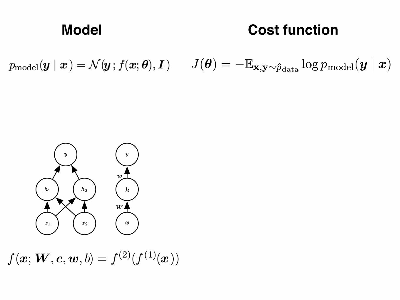
Model Cost function
CHAPTER 6. DEEP FEEDFORWARD NETWORKS
yy
hh
xx
W
w
yy
h1h1
x1x1
h2h2
x2x2
Figure 6.2: An example of a feedforward network, drawn in two different styles. Specifically,this is the feedforward network we use to solve the XOR example. It has a single hiddenlayer containing two units. (Left)In this style, we draw every unit as a node in the graph.This style is very explicit and unambiguous but for networks larger than this exampleit can consume too much space. (Right)In this style, we draw a node in the graph foreach entire vector representing a layer’s activations. This style is much more compact.Sometimes we annotate the edges in this graph with the name of the parameters thatdescribe the relationship between two layers. Here, we indicate that a matrix W describesthe mapping from x to h, and a vector w describes the mapping from h to y. Wetypically omit the intercept parameters associated with each layer when labeling this kindof drawing.
model, we used a vector of weights and a scalar bias parameter to describe anaffine transformation from an input vector to an output scalar. Now, we describean affine transformation from a vector x to a vector h, so an entire vector of biasparameters is needed. The activation function g is typically chosen to be a functionthat is applied element-wise, with hi = g(x>
W:,i + ci). In modern neural networks,the default recommendation is to use the rectified linear unit or ReLU (Jarrettet al., 2009; Nair and Hinton, 2010; Glorot et al., 2011a) defined by the activationfunction g(z) = max{0, z} depicted in figure 6.3.
We can now specify our complete network as
f(x; W , c, w, b) = w> max{0, W >
x + c} + b. (6.3)
We can now specify a solution to the XOR problem. Let
W =
1 11 1
�, (6.4)
c =
0
�1
�, (6.5)
174
Data Model Cost function Optimization
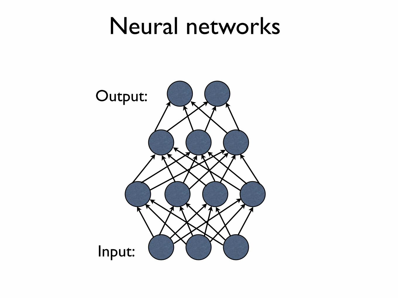
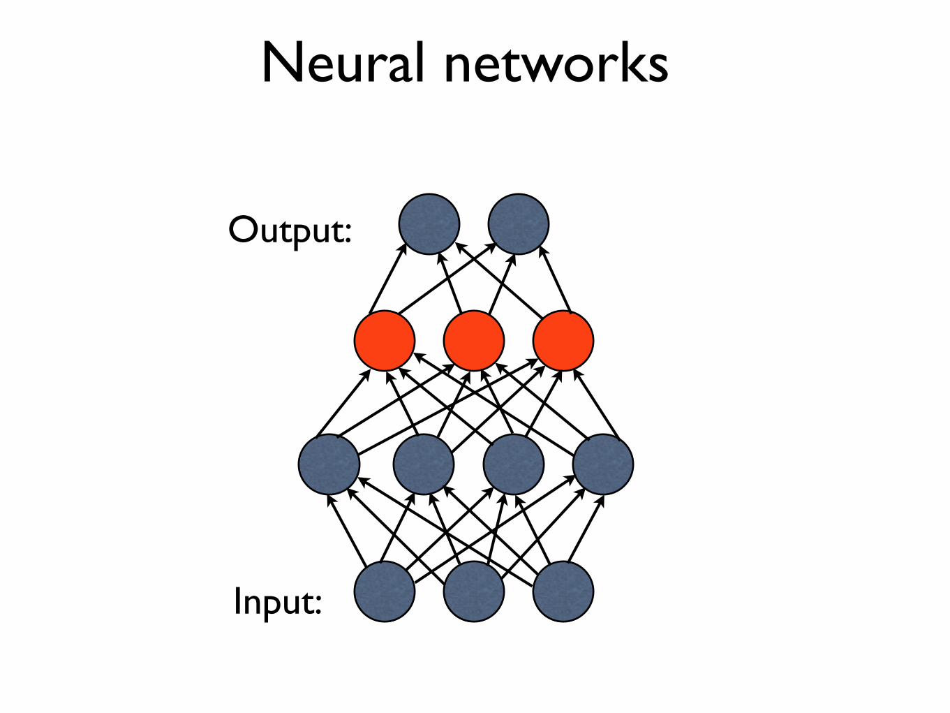
Neural networks
Input:
Output:
Neural networks
Input:
Output:
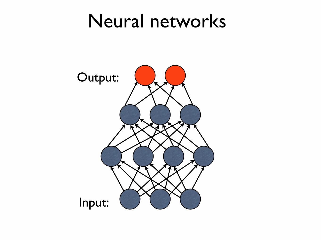
Neural networks
Input:
Output:
Neural networks
Input:
Output:
Input:
Output:
Neural networks
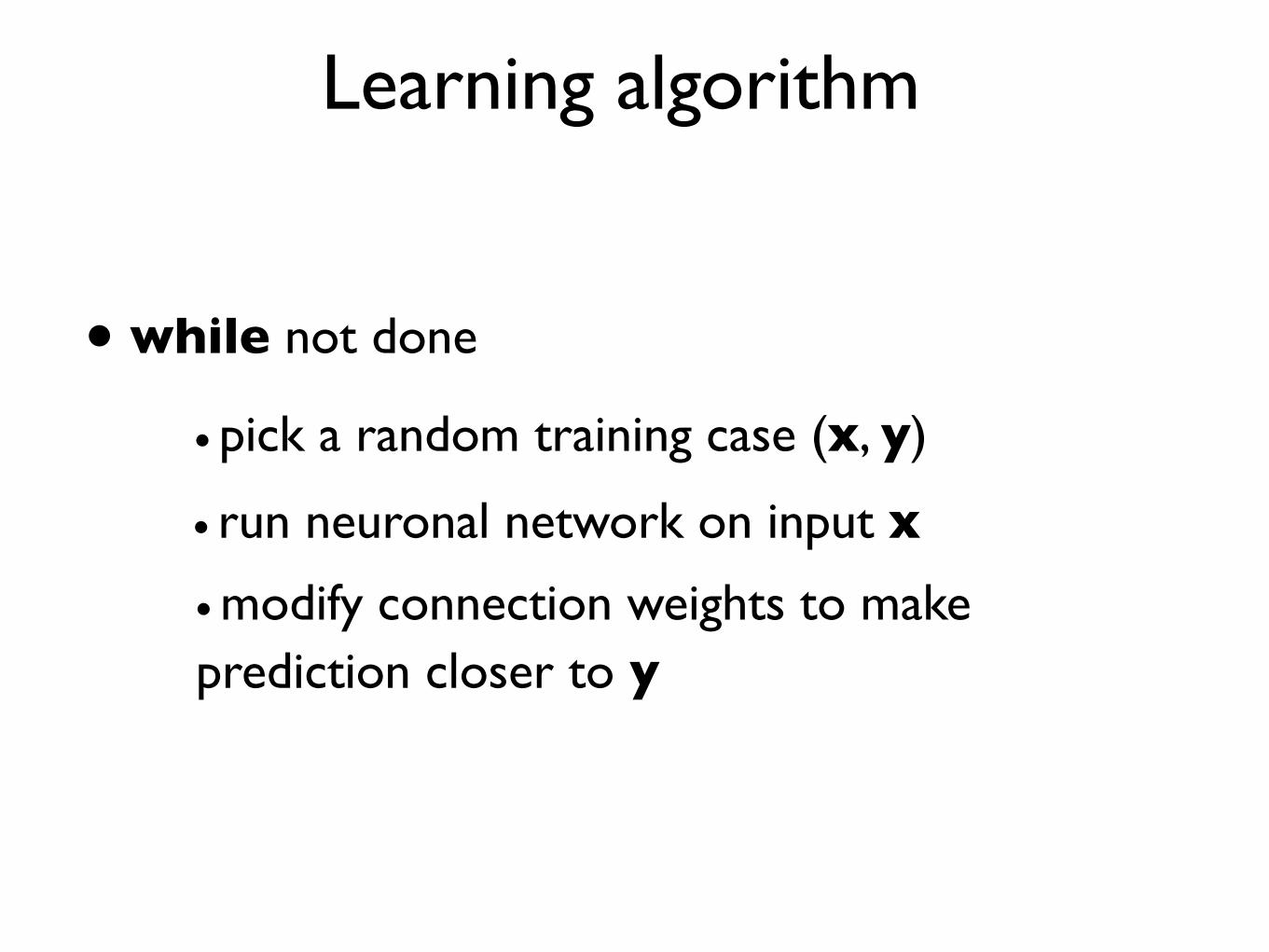
Learning algorithm
• modify connection weights to make prediction closer to y
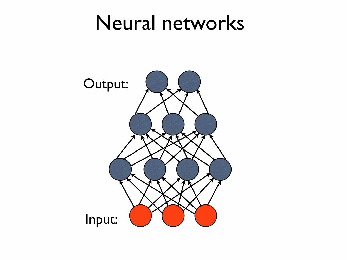
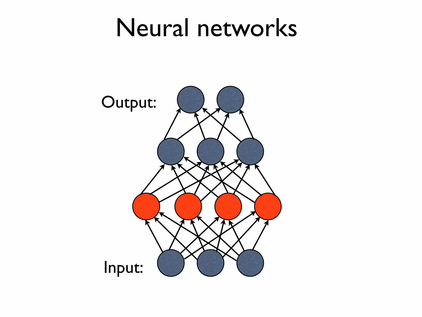
• run neuronal network on input x
• while not done
• pick a random training case (x, y)
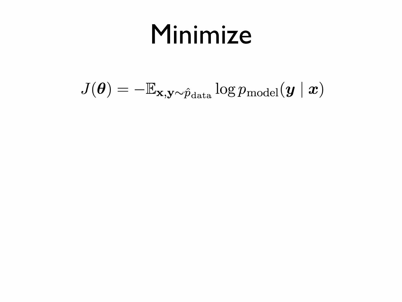
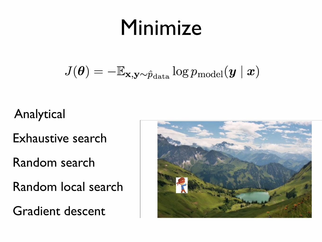
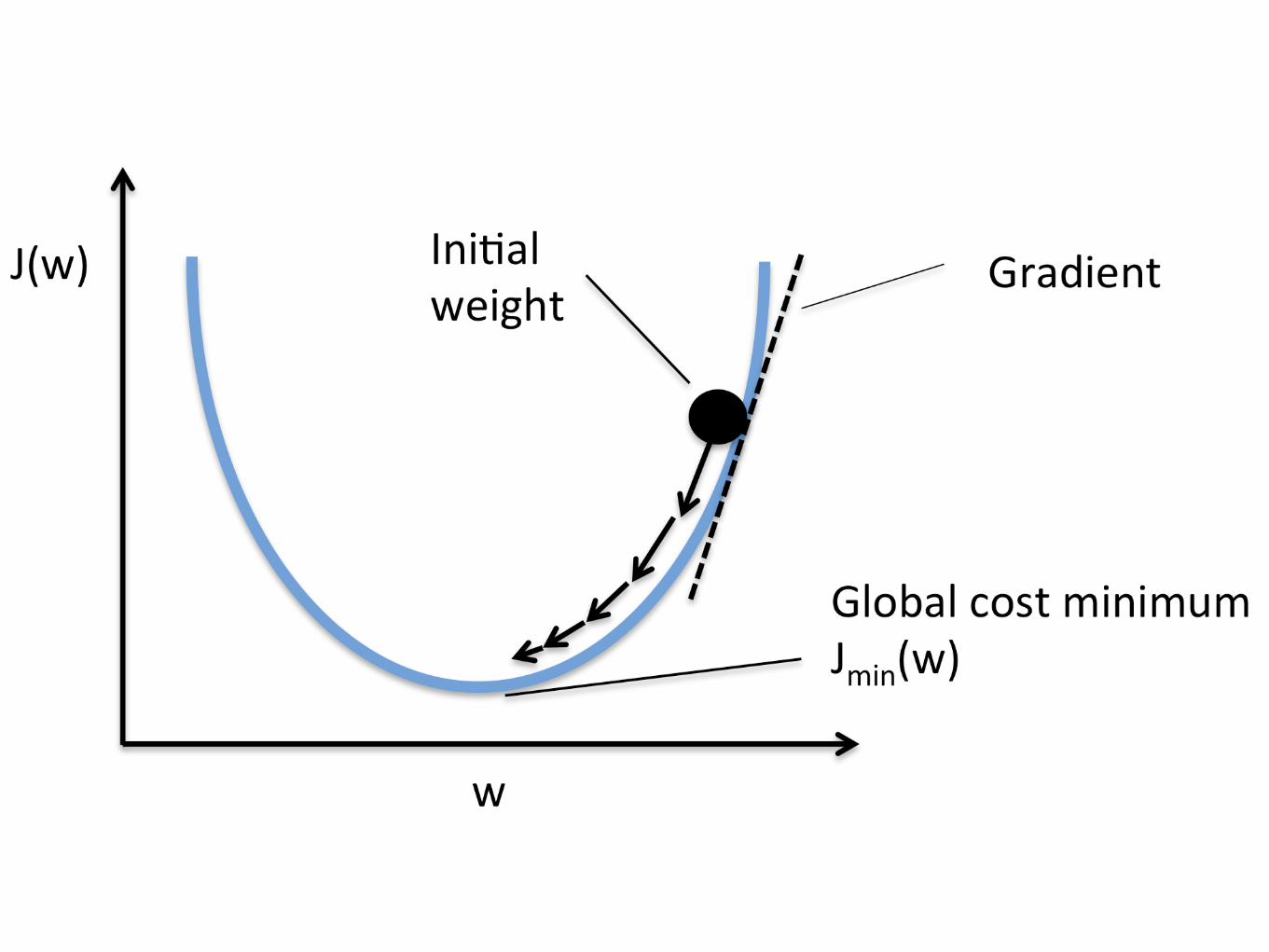
Minimize
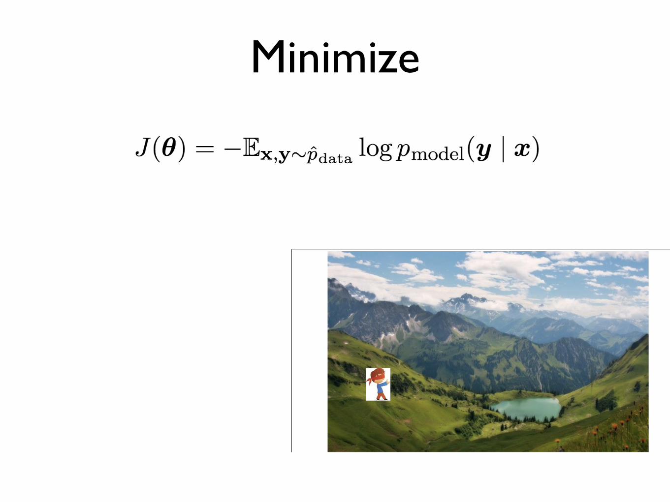
Minimize
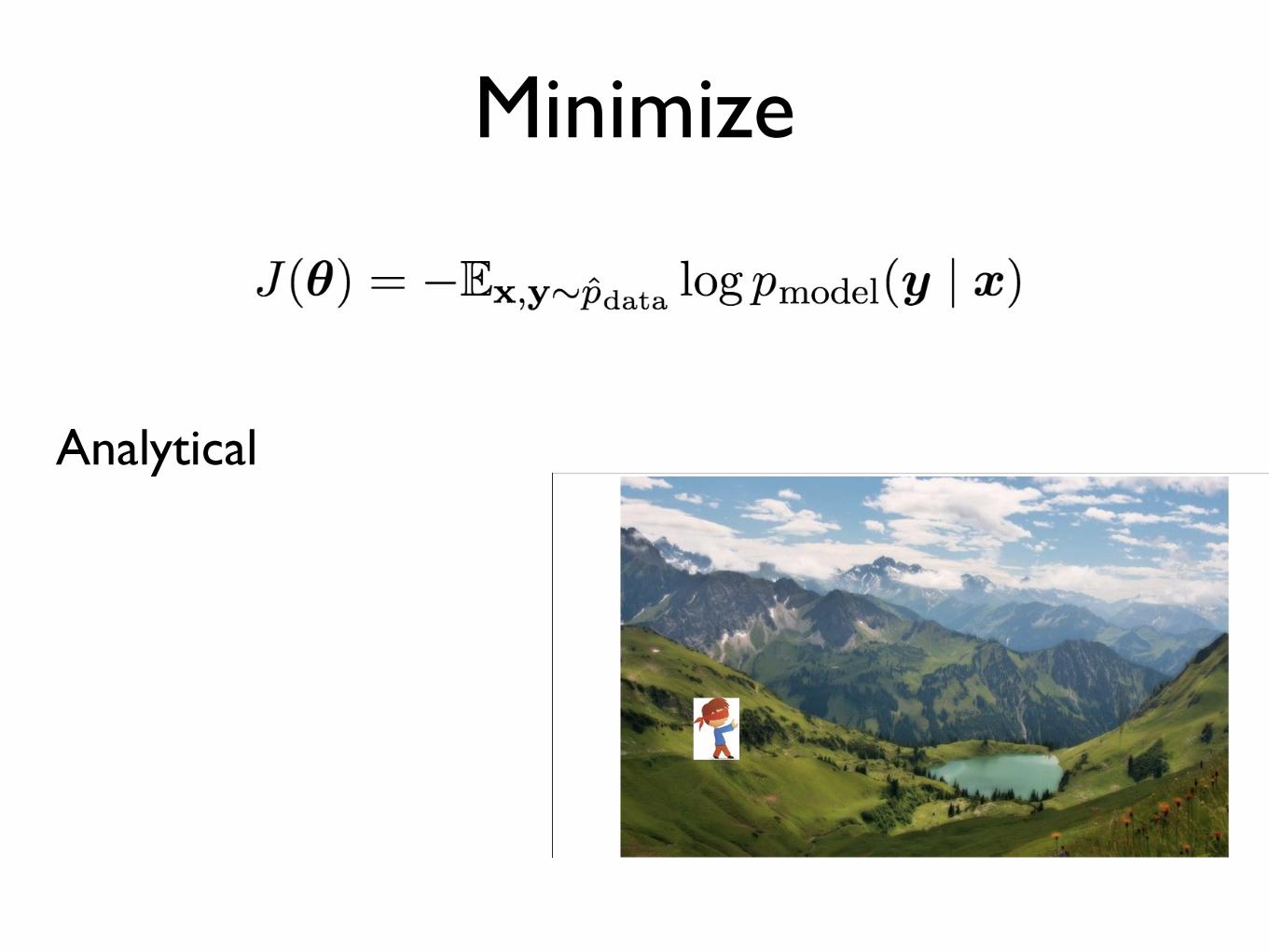
Minimize
Analytical
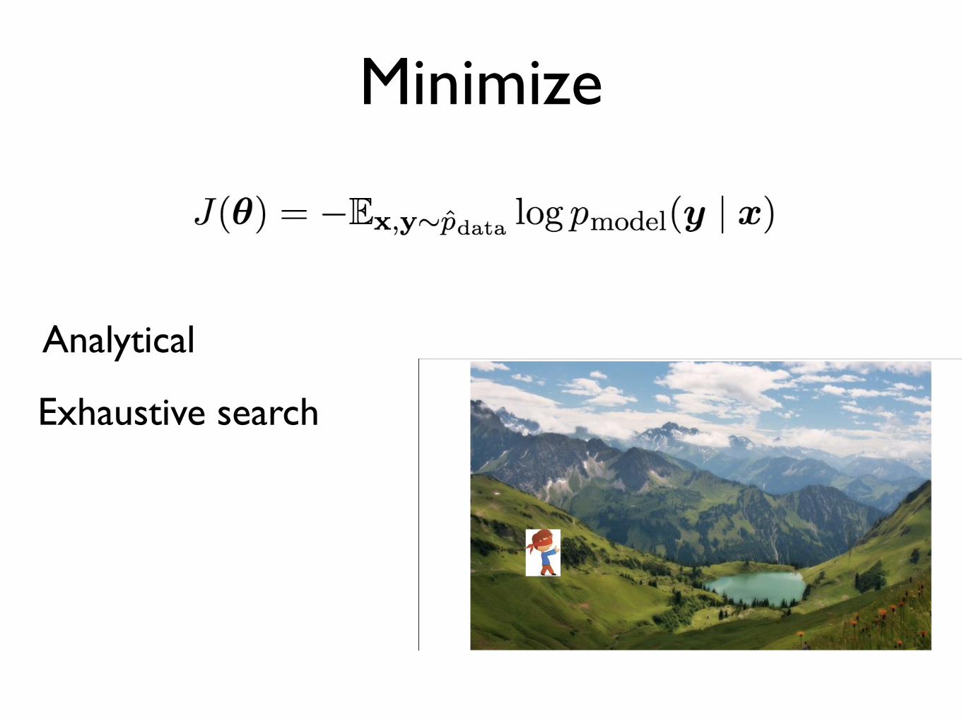
Minimize
Exhaustive search
Analytical

Minimize
Exhaustive search
Random search
Analytical
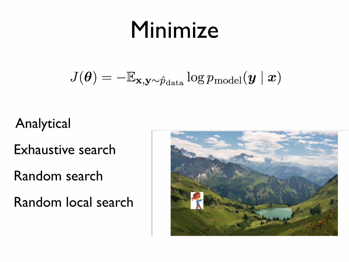
Minimize
Exhaustive search
Random search
Random local search
Analytical
Minimize
Exhaustive search
Random search
Random local search
Gradient descent
Analytical
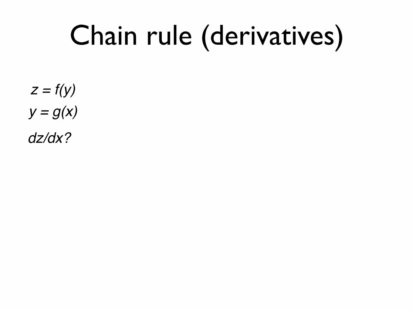
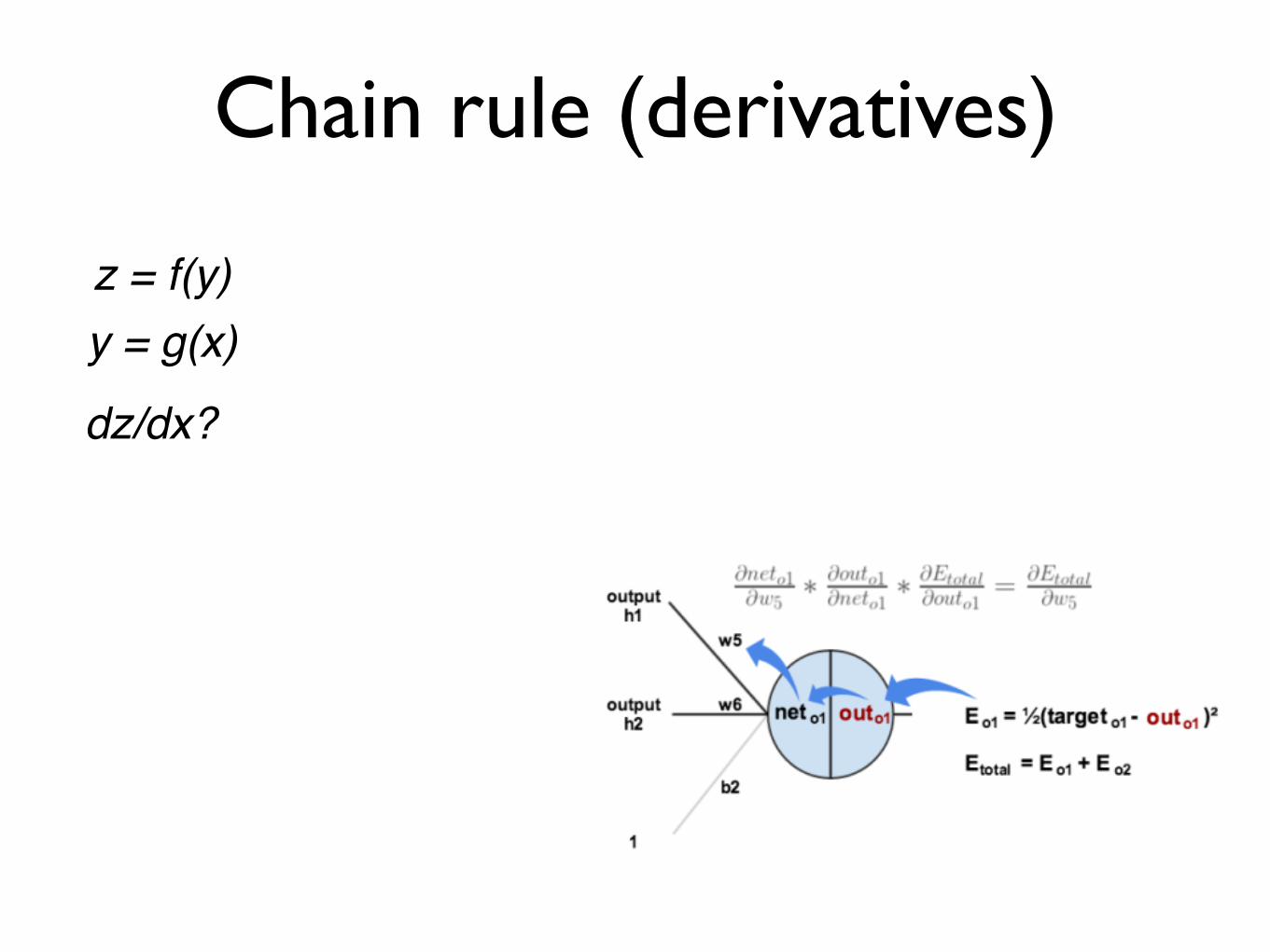
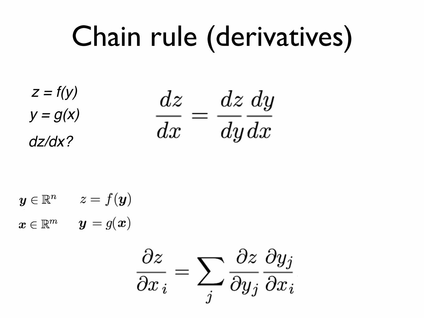
Chain rule (derivatives)
z = f(y)y = g(x)
dz/dx?
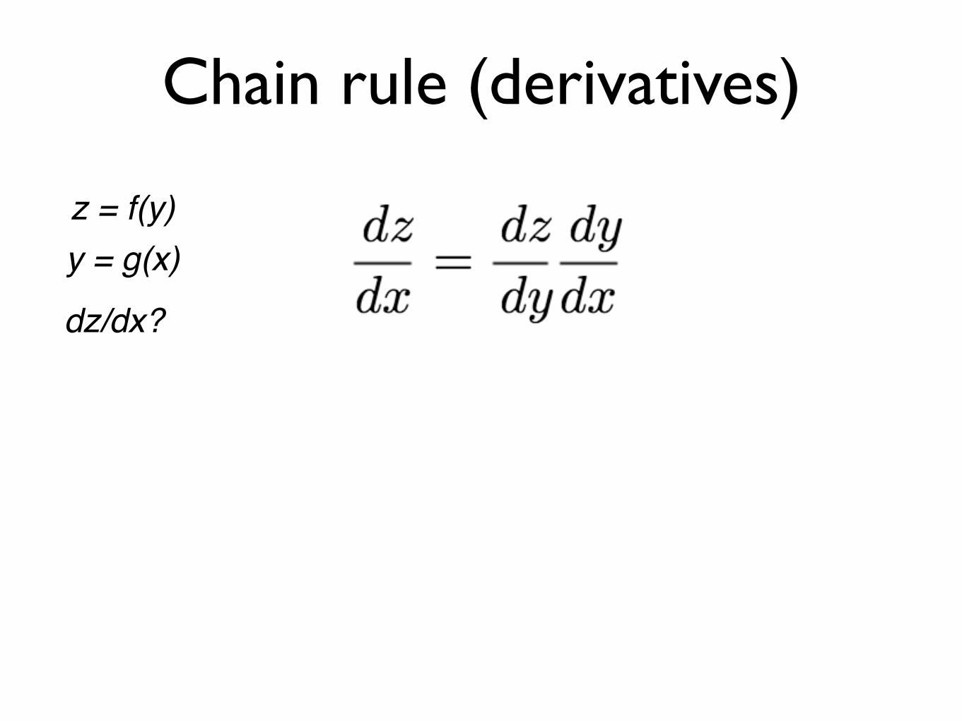
Chain rule (derivatives)
z = f(y)y = g(x)
dz/dx?
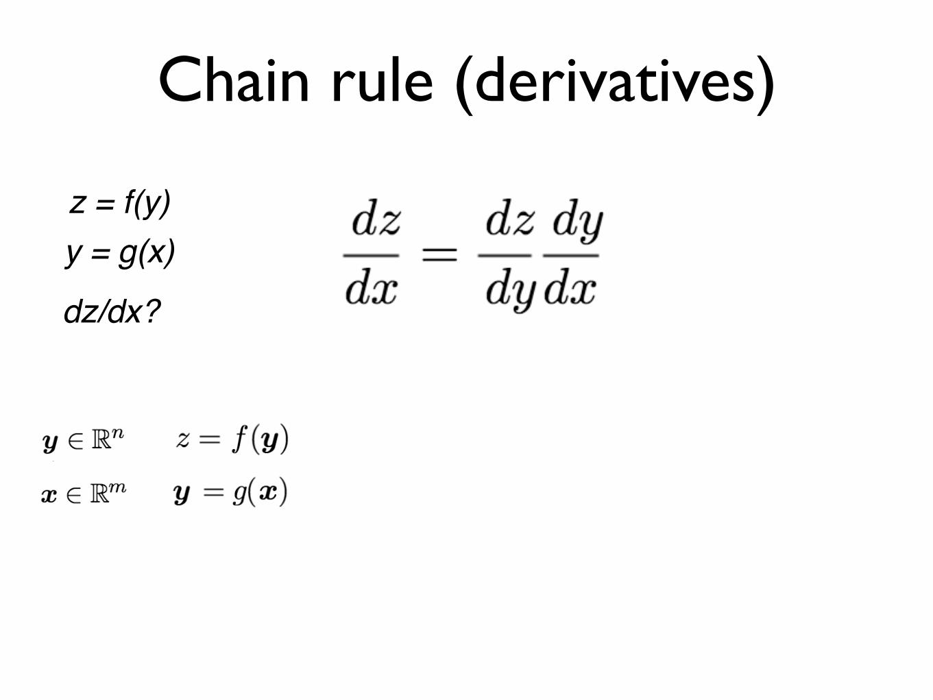
Chain rule (derivatives)
z = f(y)y = g(x)
dz/dx?
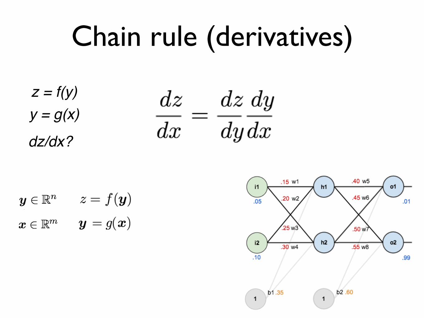
Chain rule (derivatives)
z = f(y)y = g(x)
dz/dx?
Chain rule (derivatives)
z = f(y)y = g(x)
dz/dx?
Chain rule (derivatives)
z = f(y)y = g(x)
dz/dx?
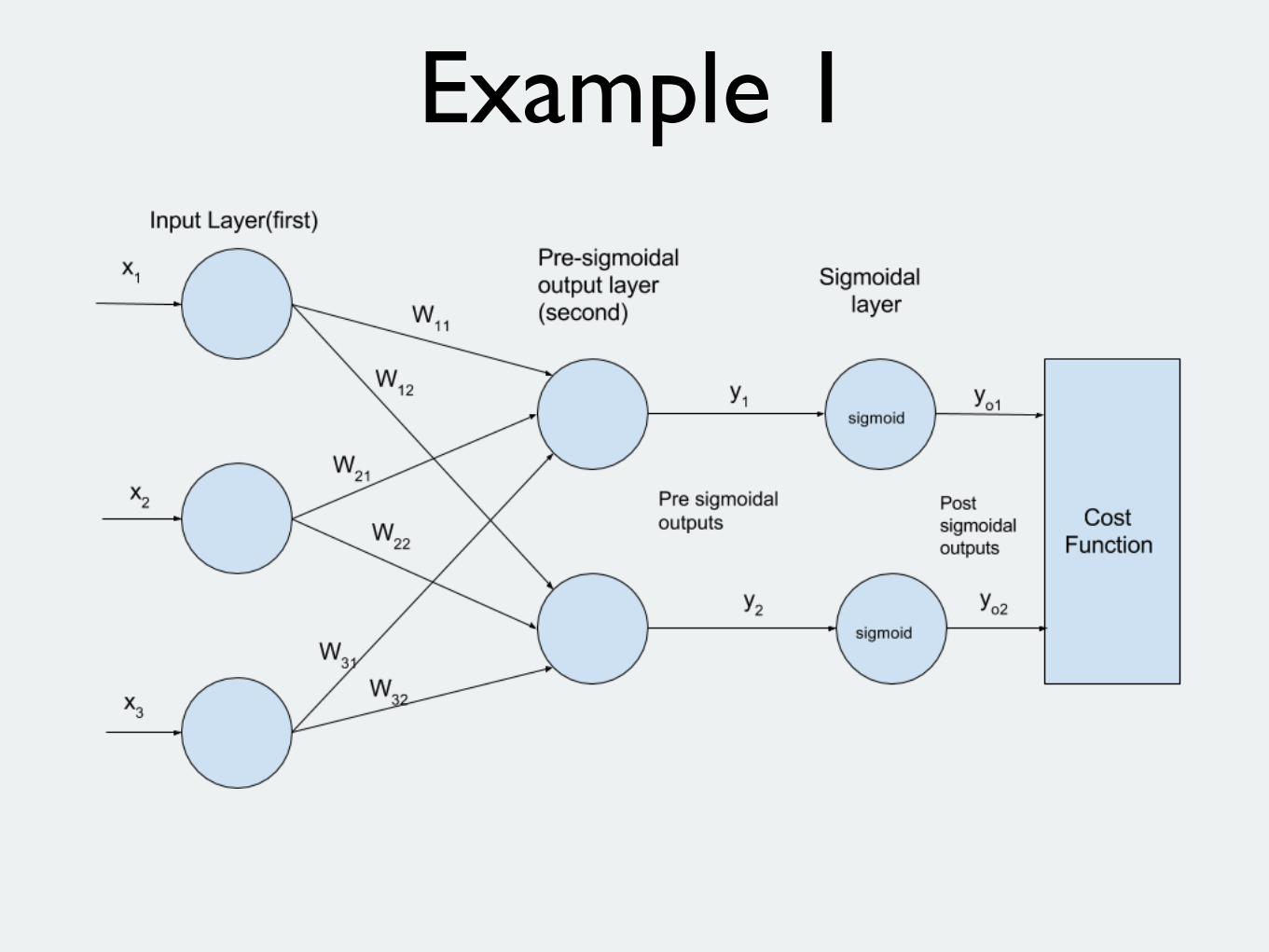
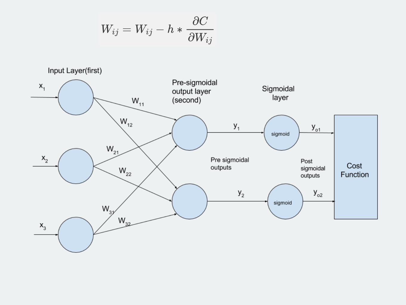
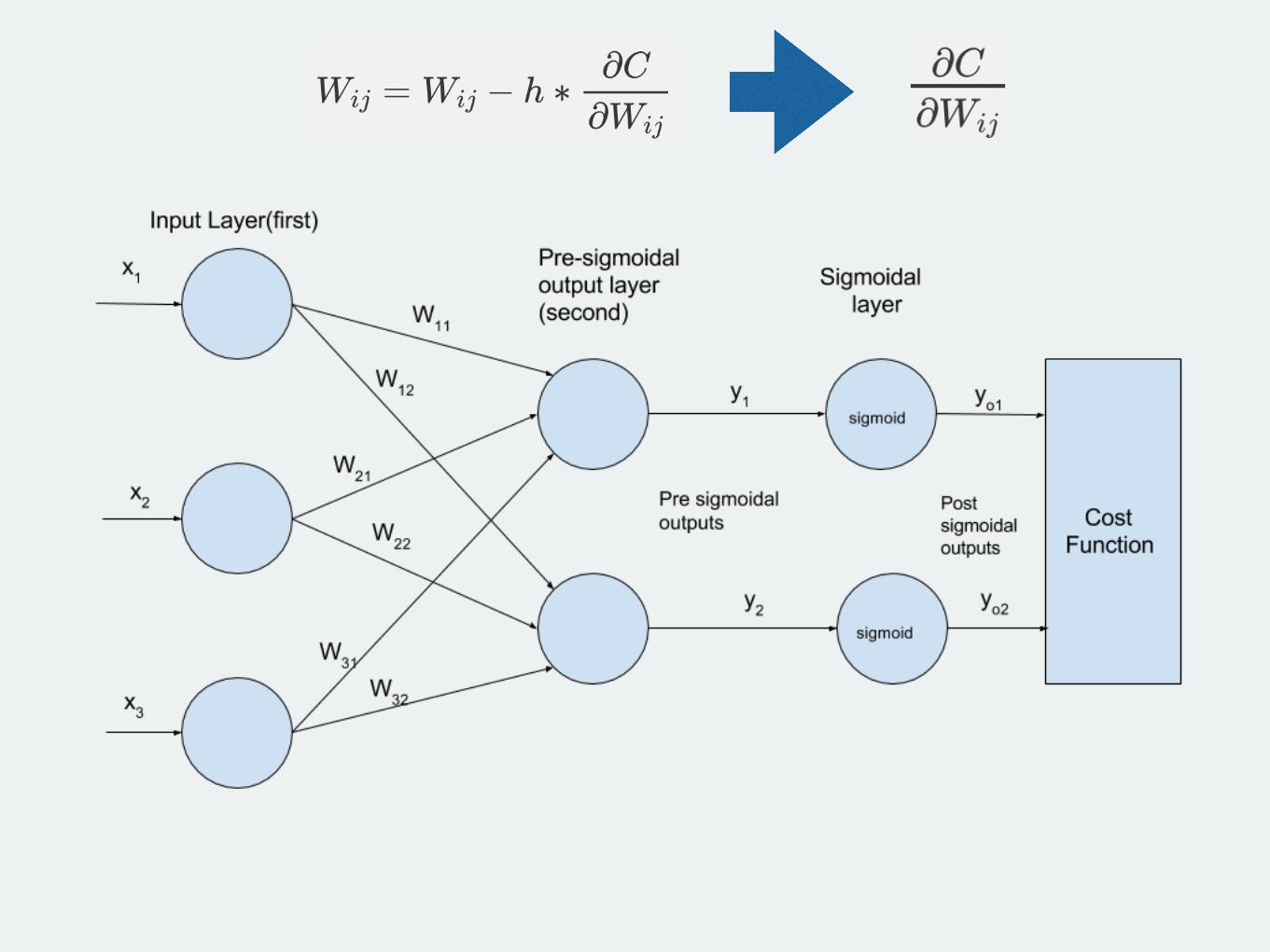
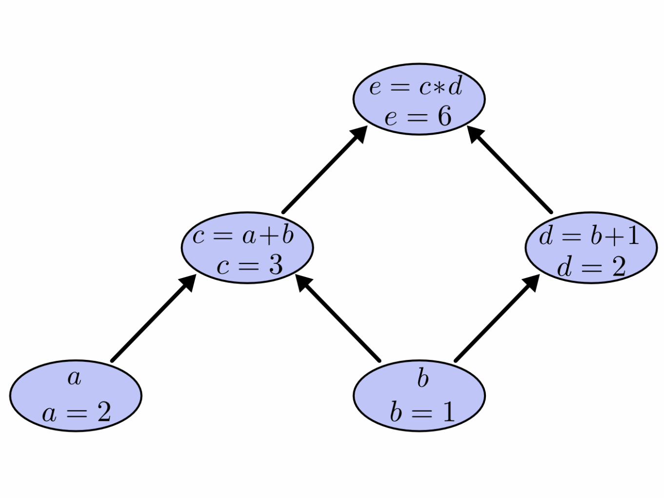
Example 1

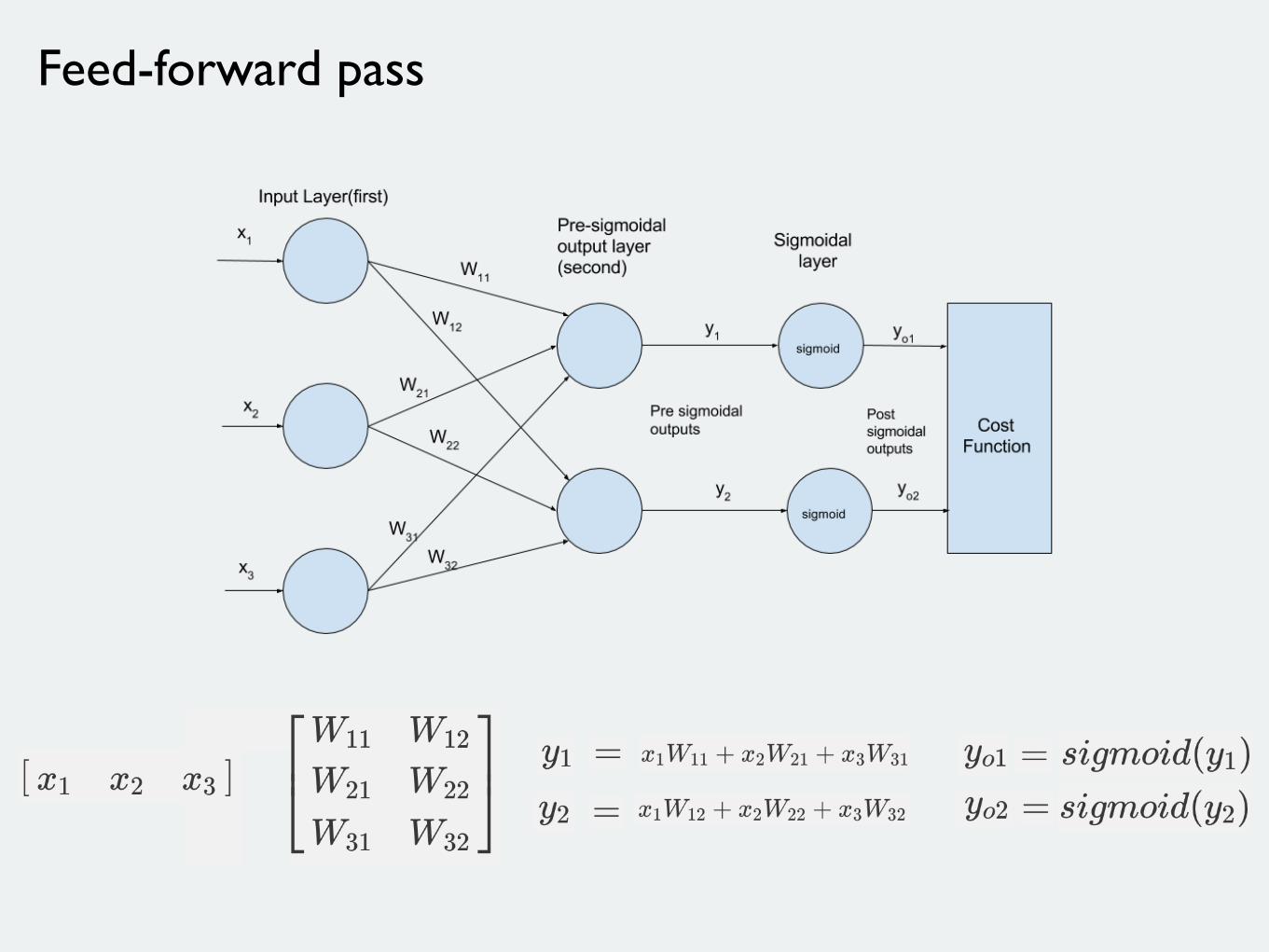
Feed-forward pass
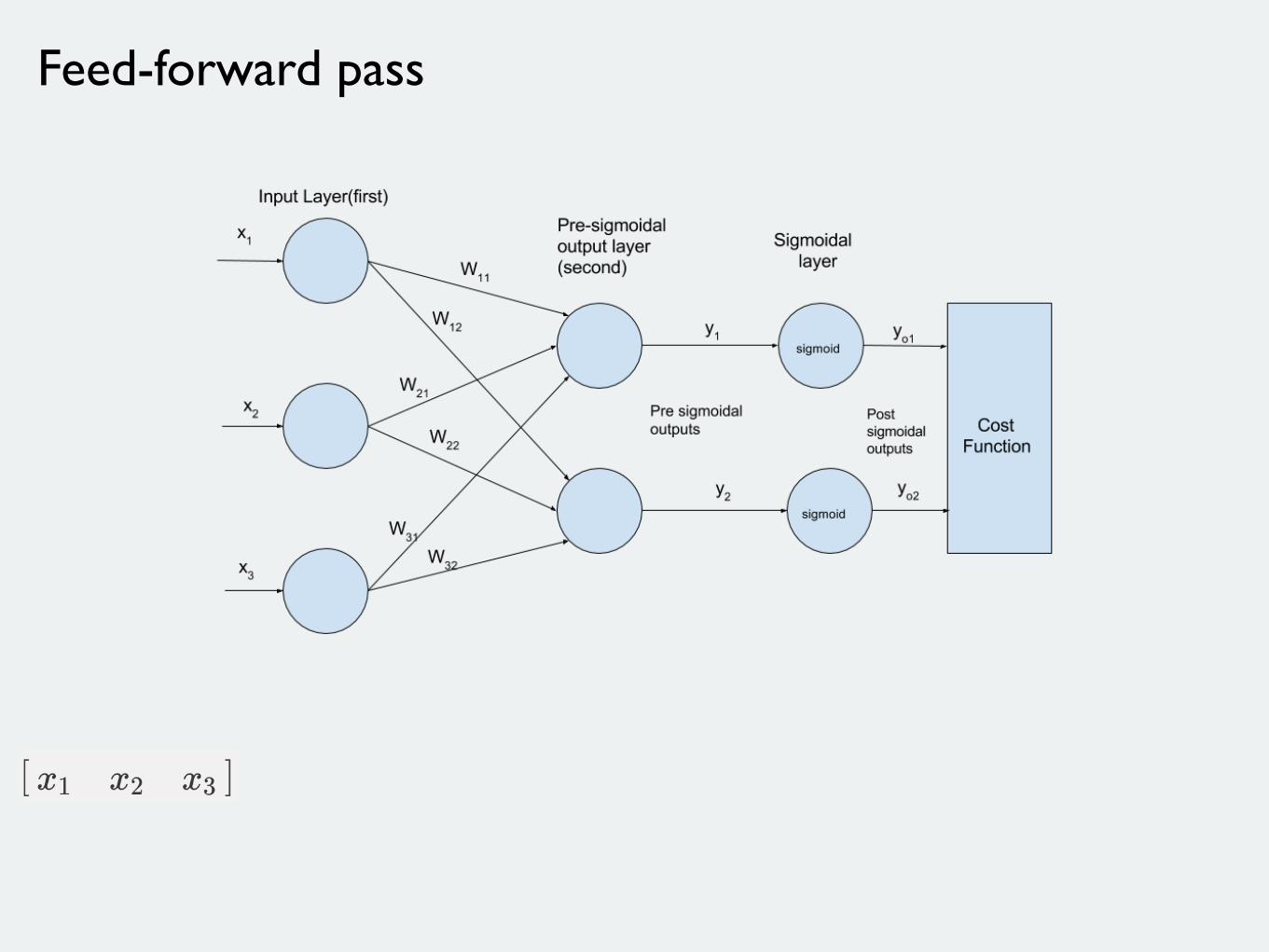
Feed-forward pass
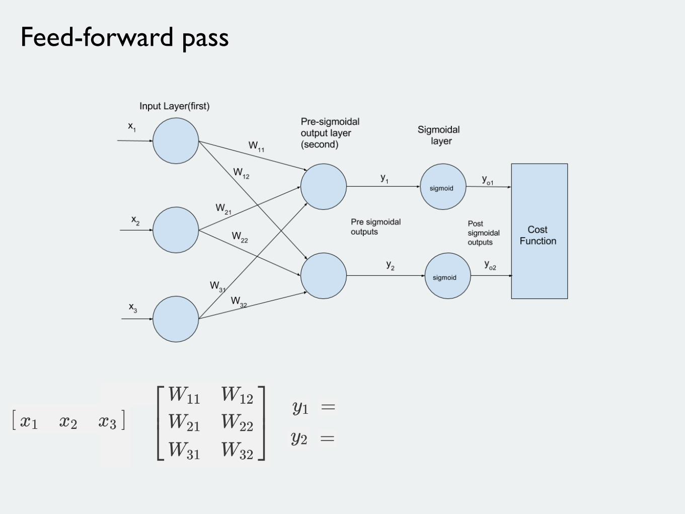
Feed-forward pass
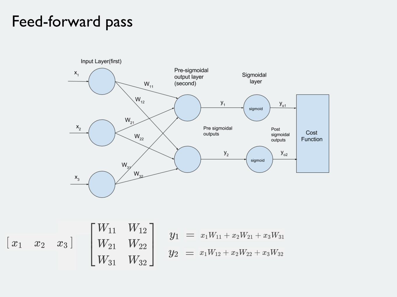
Feed-forward pass
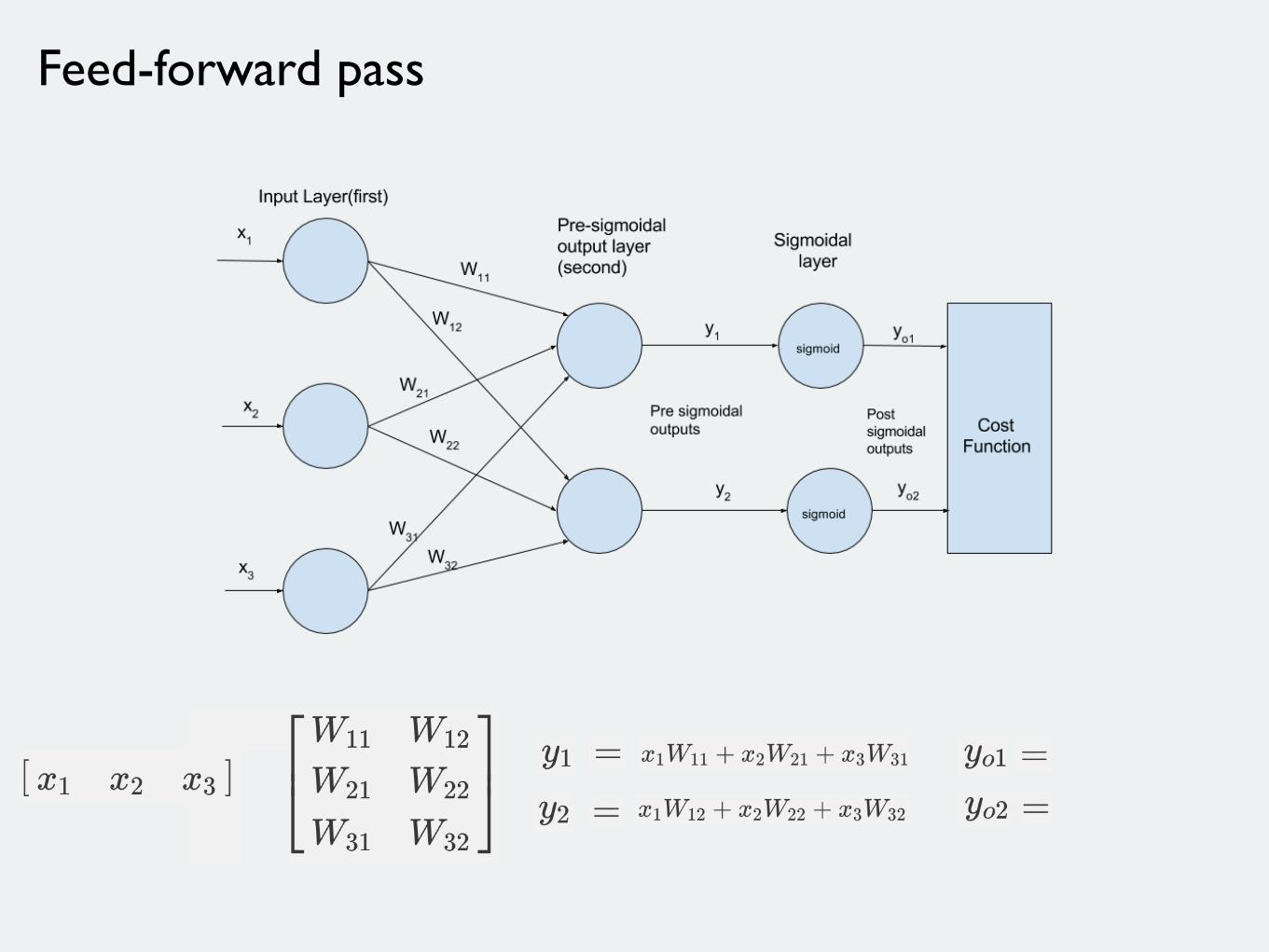
Feed-forward pass
Feed-forward pass
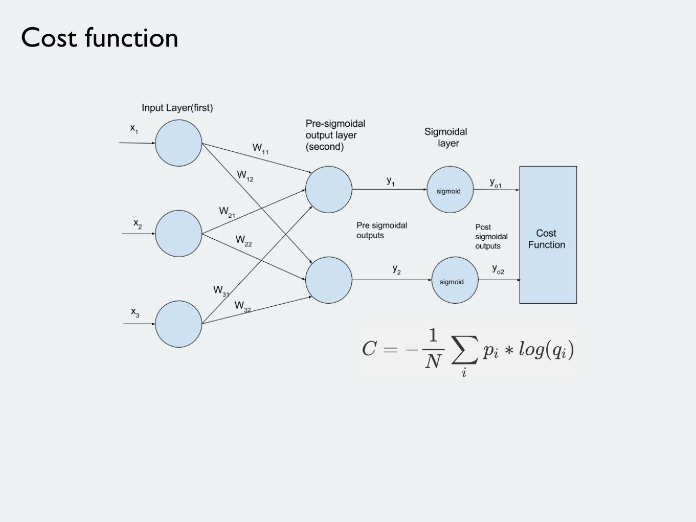
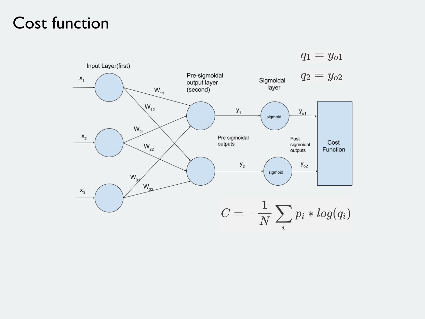
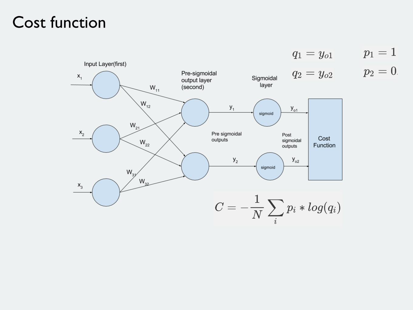
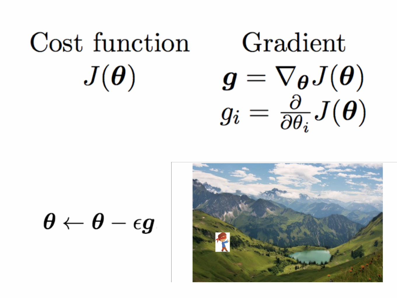
Cost function
Cost function
Cost function
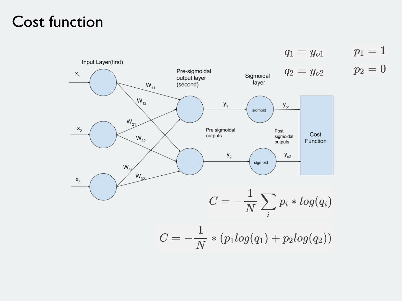
Cost function
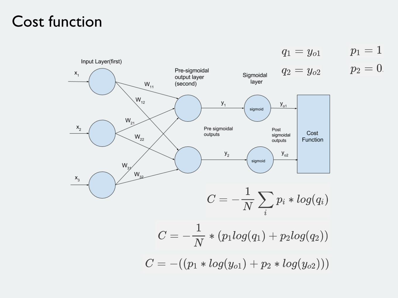
Cost function
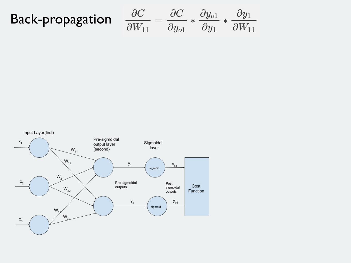
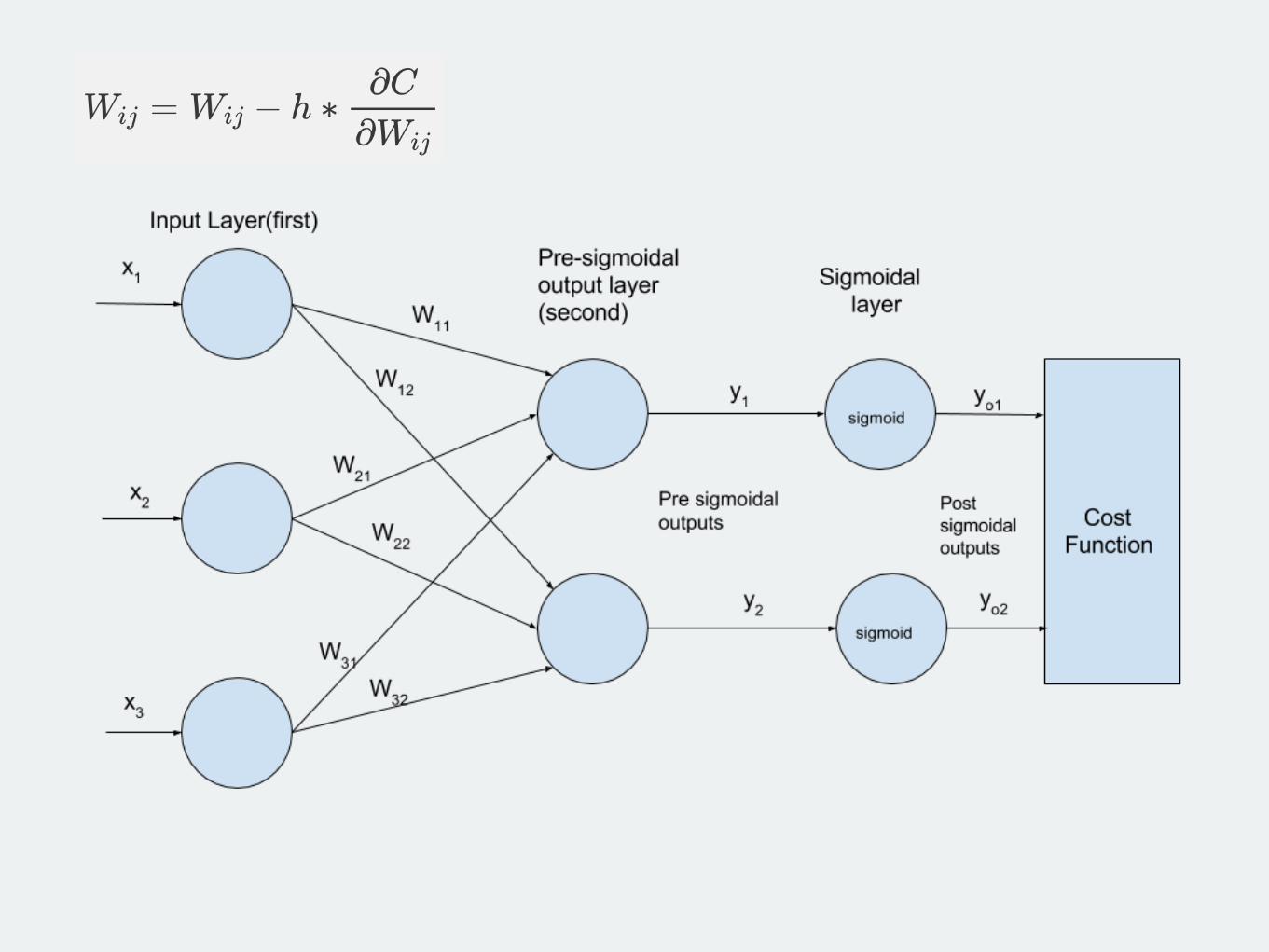
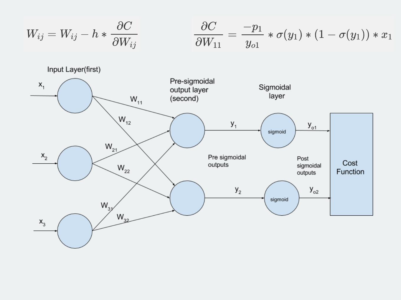
Back-propagation
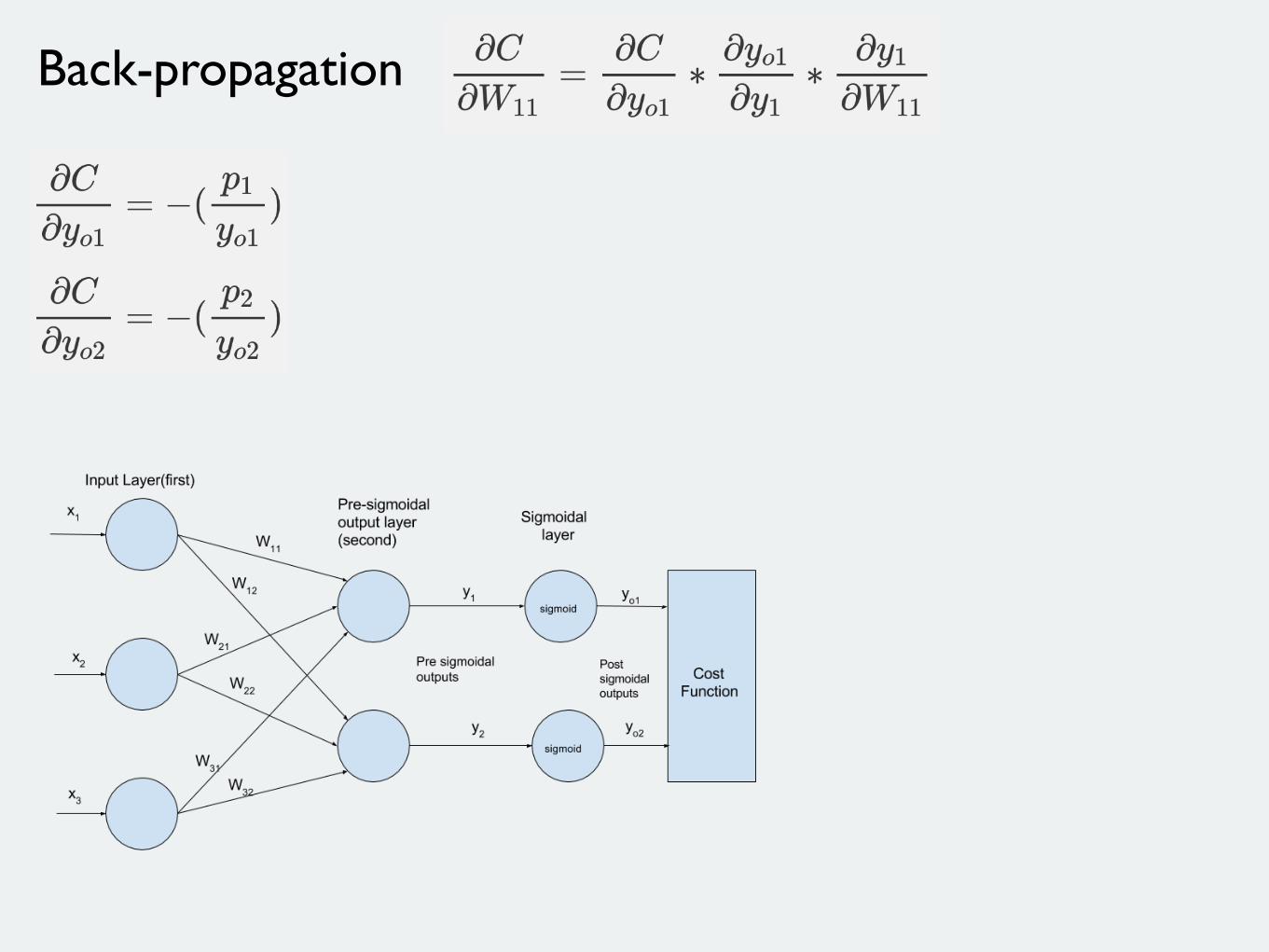
Back-propagation
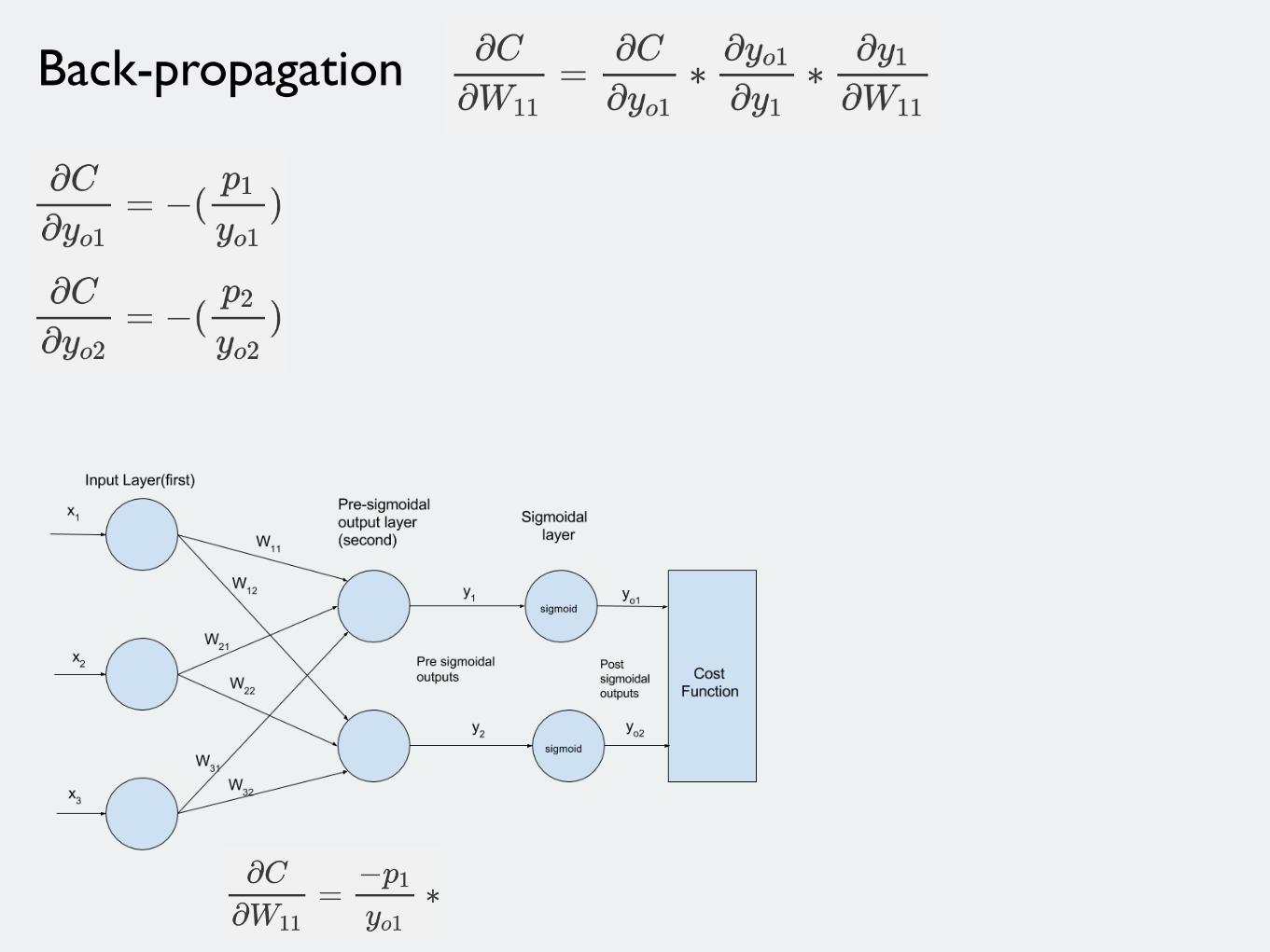
Back-propagation
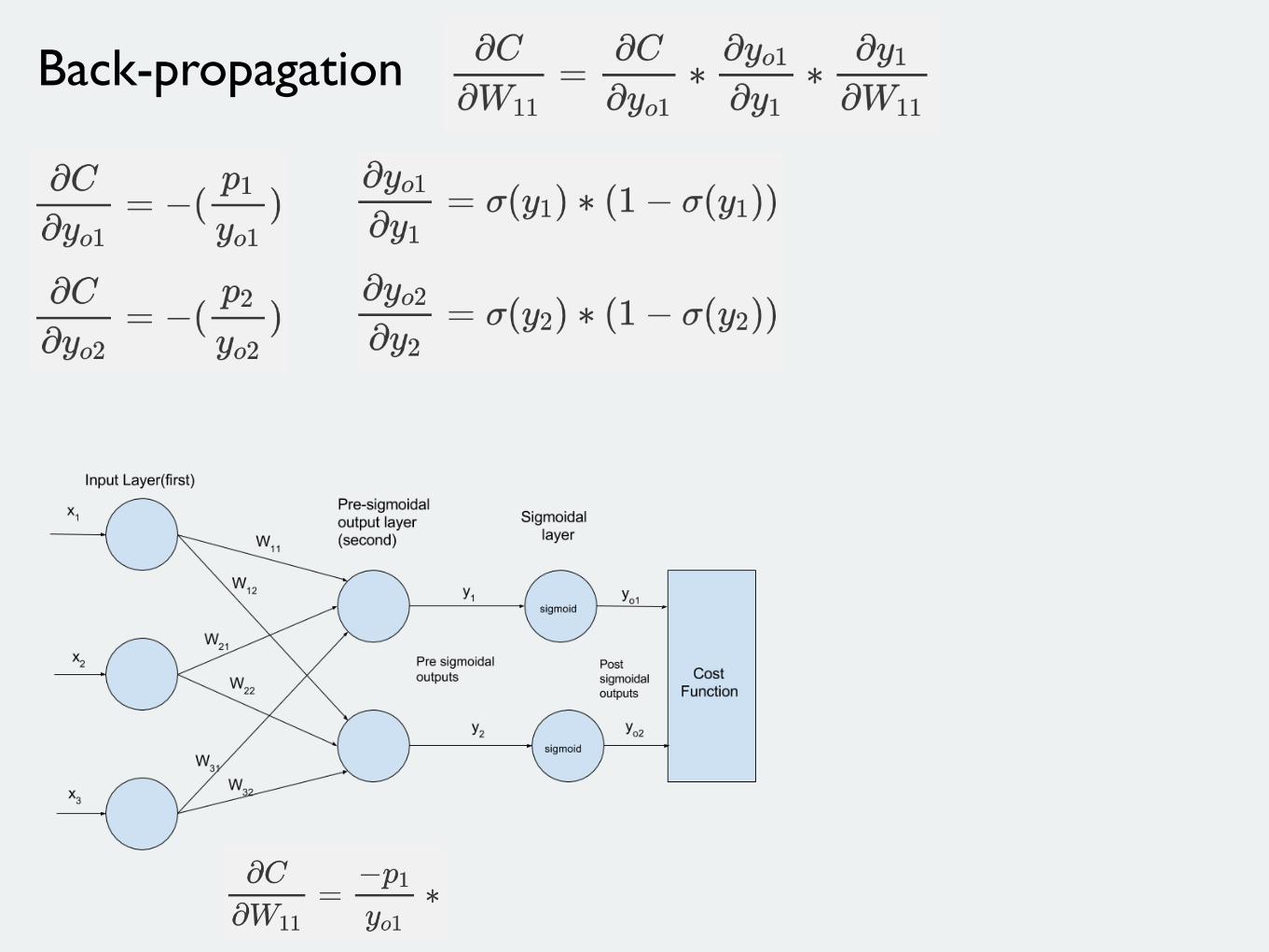
Back-propagation
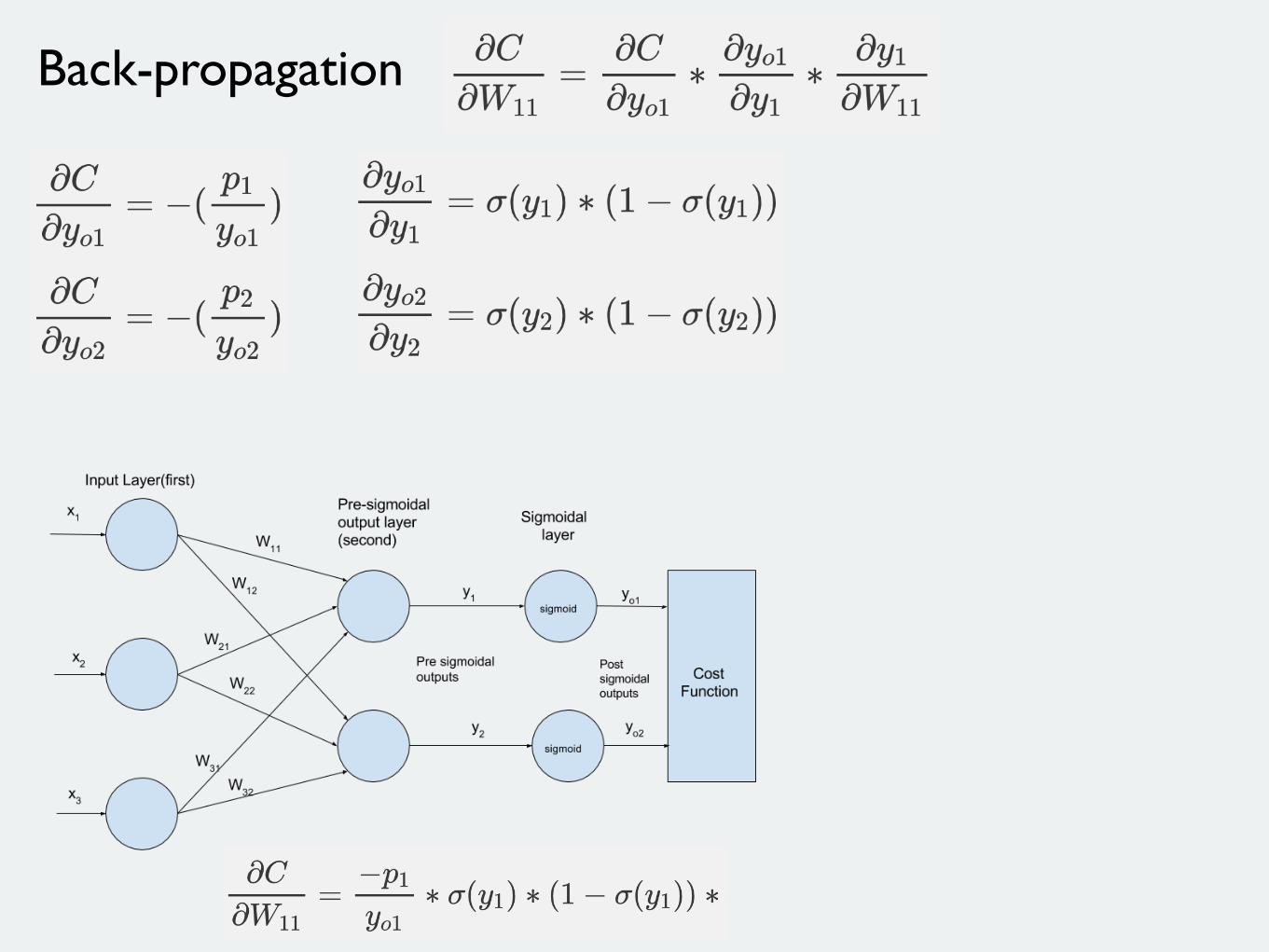
Back-propagation
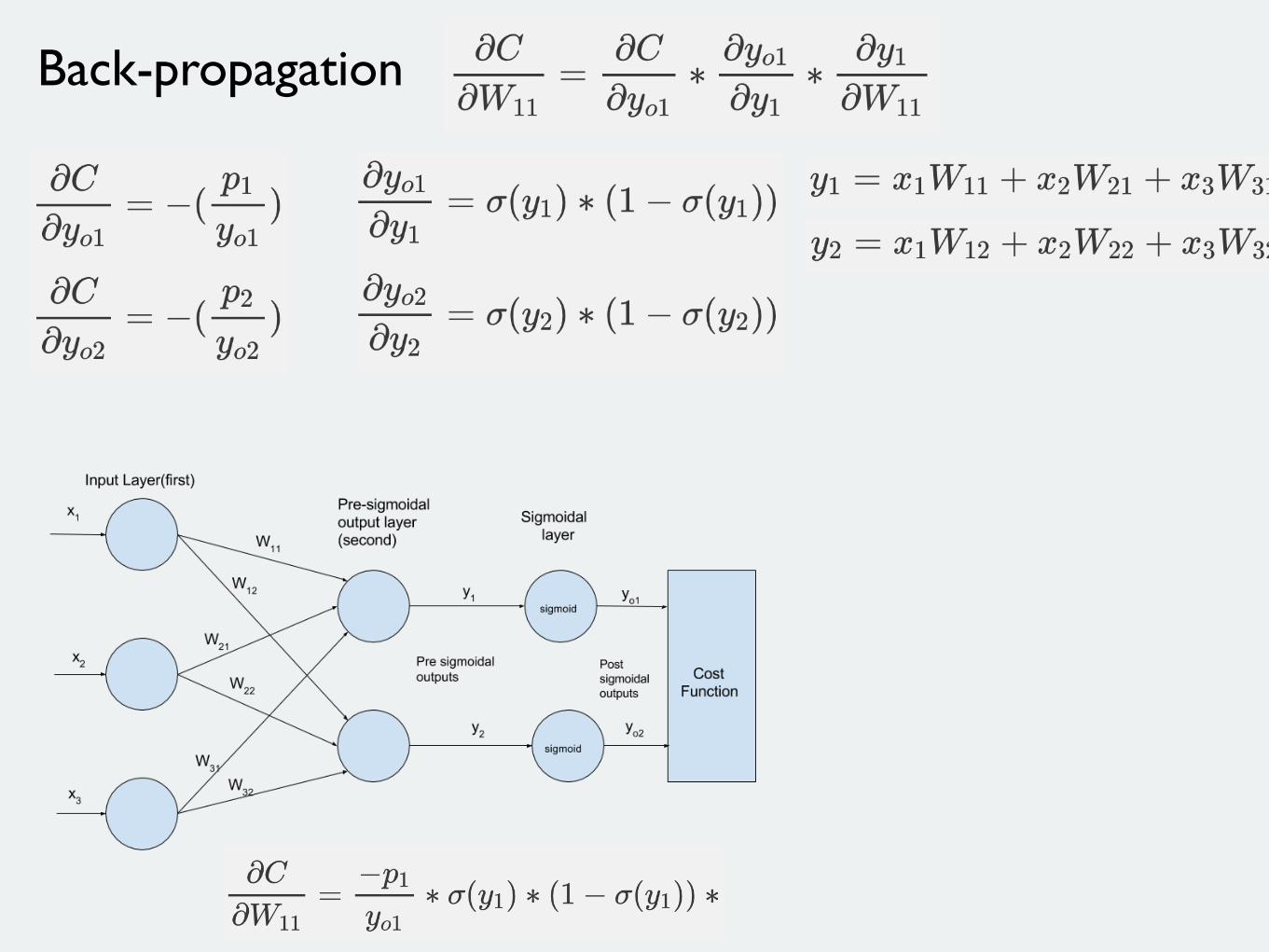
Back-propagation
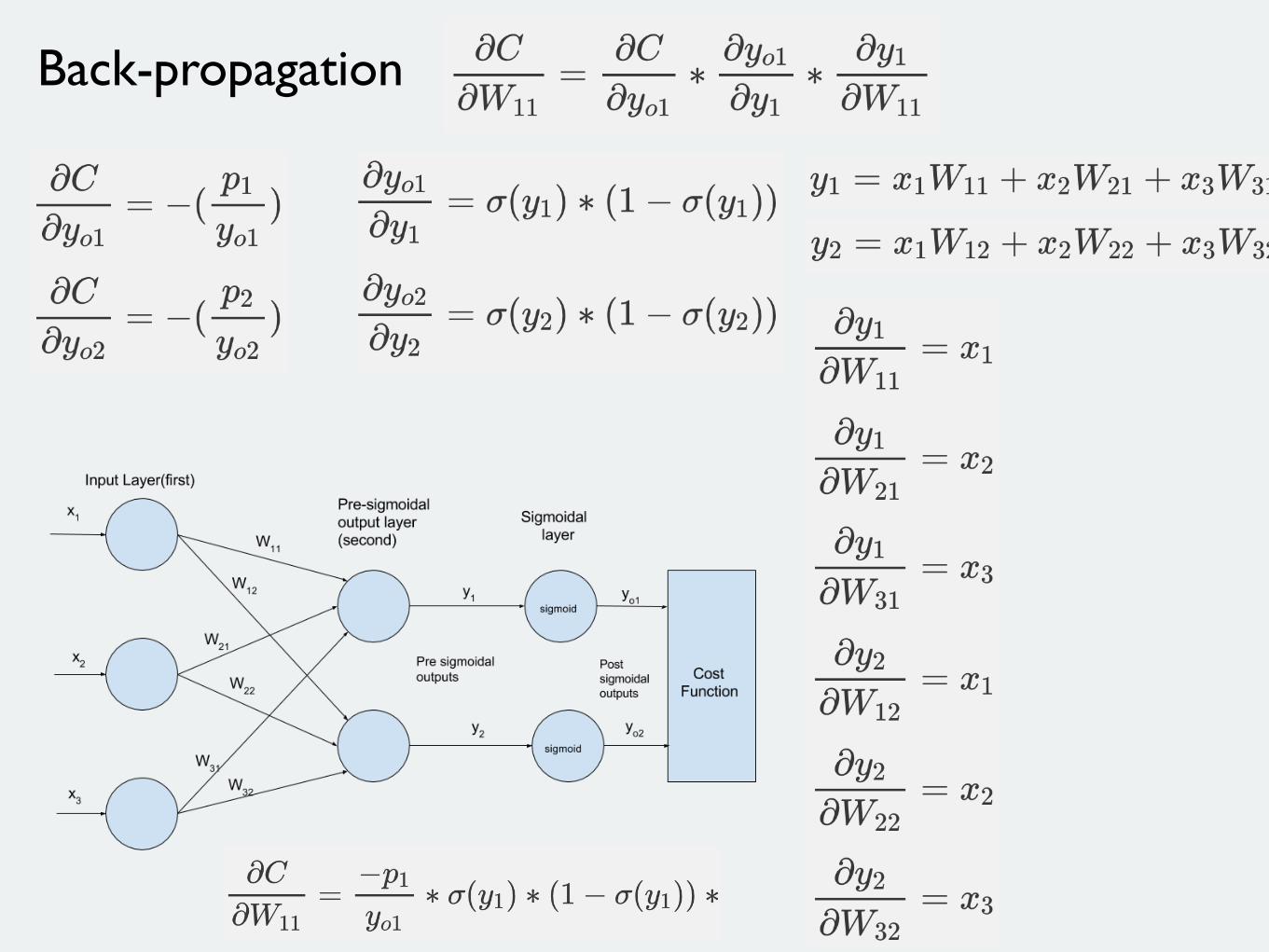
Back-propagation
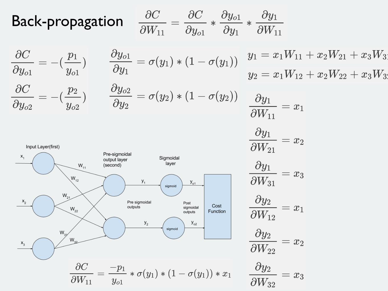
Back-propagation
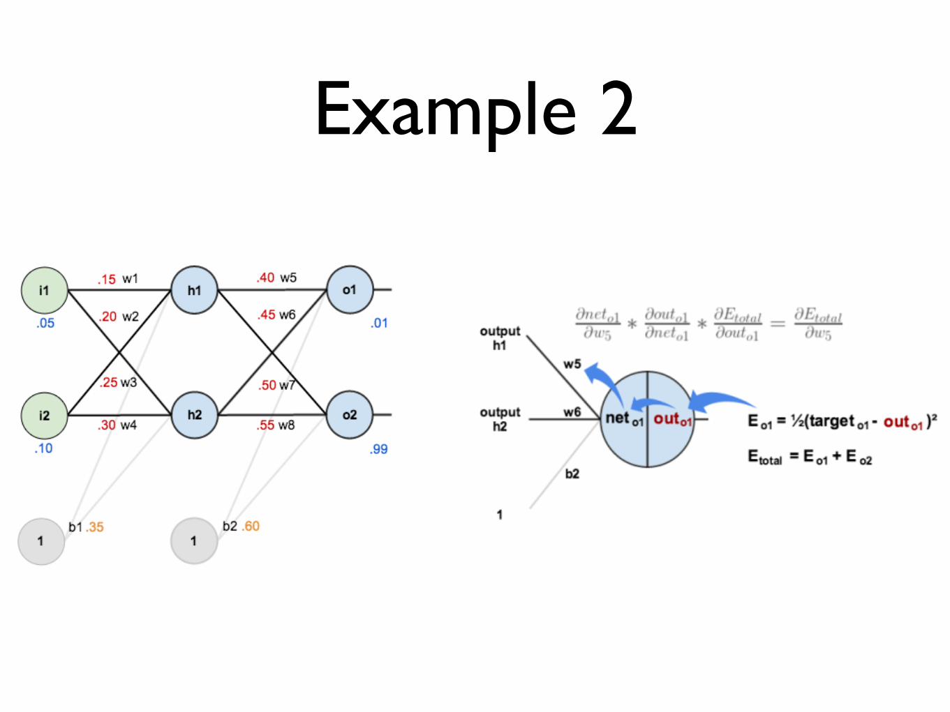
Example 2
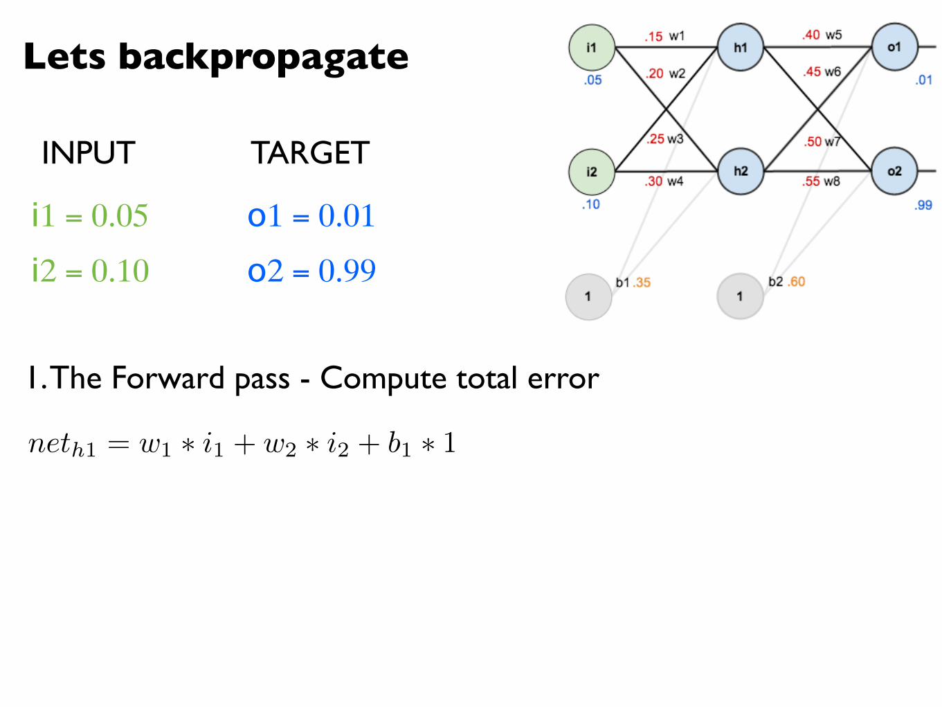
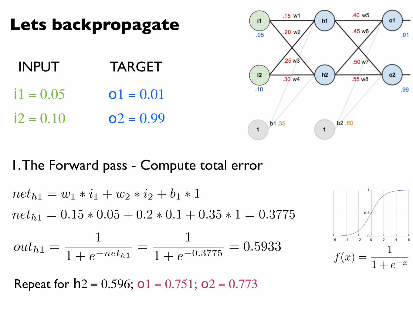
Lets backpropagate
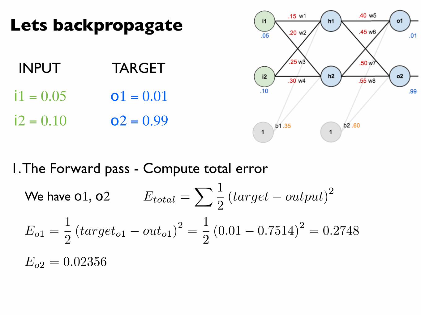
i1 = 0.05
i2 = 0.10
o1 = 0.01
o2 = 0.99
1. The Forward pass - Compute total error
neth1 = w1 ⇤ i1 + w2 ⇤ i2 + b1 ⇤ 1
INPUT TARGET
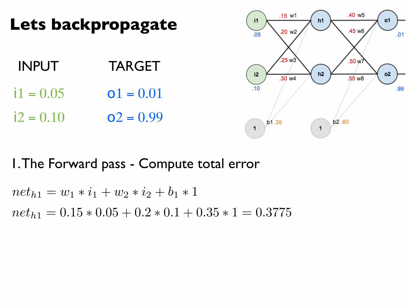
Lets backpropagate
i1 = 0.05
i2 = 0.10
o1 = 0.01
o2 = 0.99
1. The Forward pass - Compute total error
neth1 = w1 ⇤ i1 + w2 ⇤ i2 + b1 ⇤ 1neth1 = 0.15 ⇤ 0.05 + 0.2 ⇤ 0.1 + 0.35 ⇤ 1 = 0.3775
INPUT TARGET
Lets backpropagate
i1 = 0.05
i2 = 0.10
o1 = 0.01
o2 = 0.99
1. The Forward pass - Compute total error
neth1 = w1 ⇤ i1 + w2 ⇤ i2 + b1 ⇤ 1neth1 = 0.15 ⇤ 0.05 + 0.2 ⇤ 0.1 + 0.35 ⇤ 1 = 0.3775
INPUT TARGET
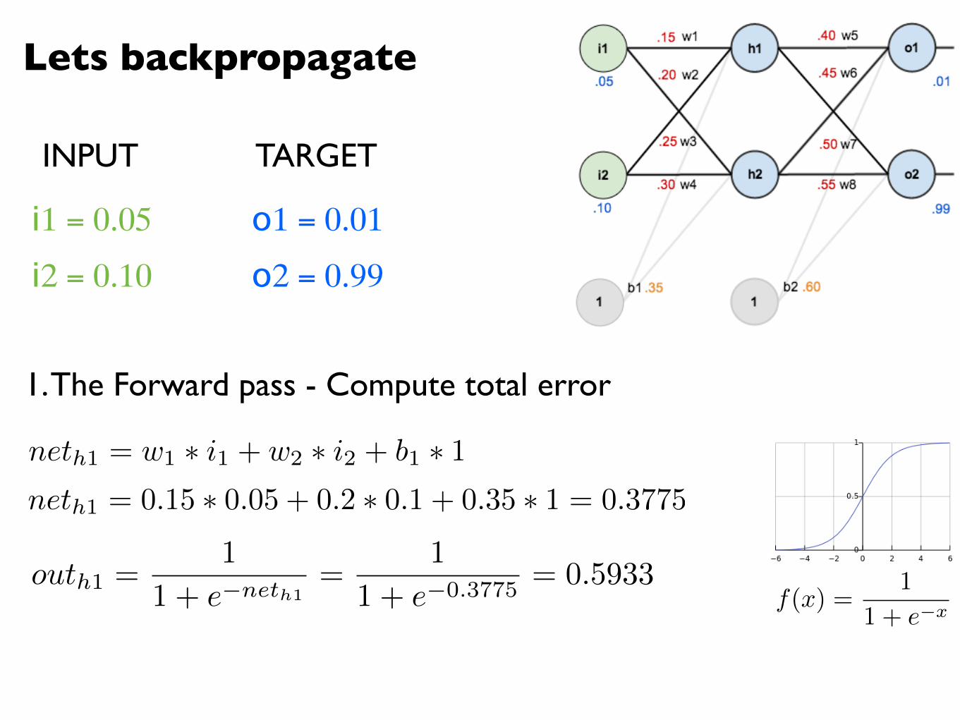
f(x) =1
1 + e�x
outh1 =1
1 + e�neth1=
1
1 + e�0.3775= 0.5933
Lets backpropagate
i1 = 0.05
i2 = 0.10
o1 = 0.01
o2 = 0.99
1. The Forward pass - Compute total error
neth1 = w1 ⇤ i1 + w2 ⇤ i2 + b1 ⇤ 1neth1 = 0.15 ⇤ 0.05 + 0.2 ⇤ 0.1 + 0.35 ⇤ 1 = 0.3775
INPUT TARGET
f(x) =1
1 + e�x
outh1 =1
1 + e�neth1=
1
1 + e�0.3775= 0.5933
Repeat for h2 = 0.596; o1 = 0.751; o2 = 0.773
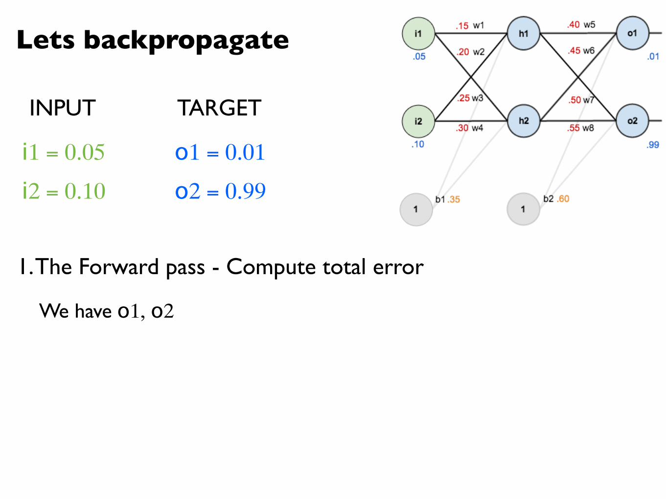
Lets backpropagate
i1 = 0.05
i2 = 0.10
o1 = 0.01
o2 = 0.99
1. The Forward pass - Compute total error
INPUT TARGET
We have o1, o2
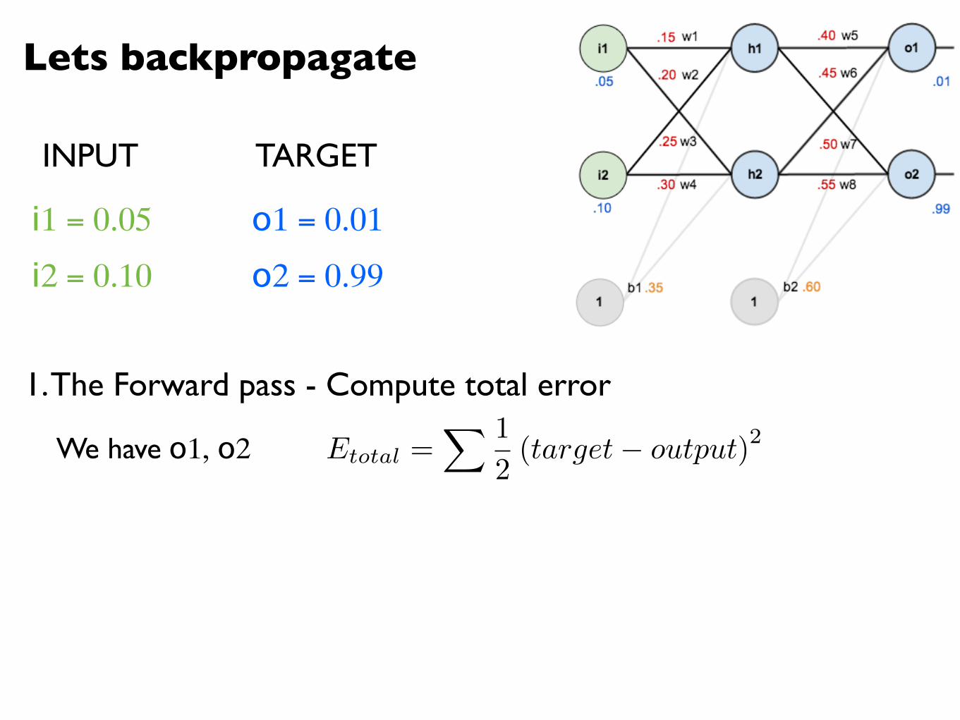
Lets backpropagate
i1 = 0.05
i2 = 0.10
o1 = 0.01
o2 = 0.99
1. The Forward pass - Compute total error
INPUT TARGET
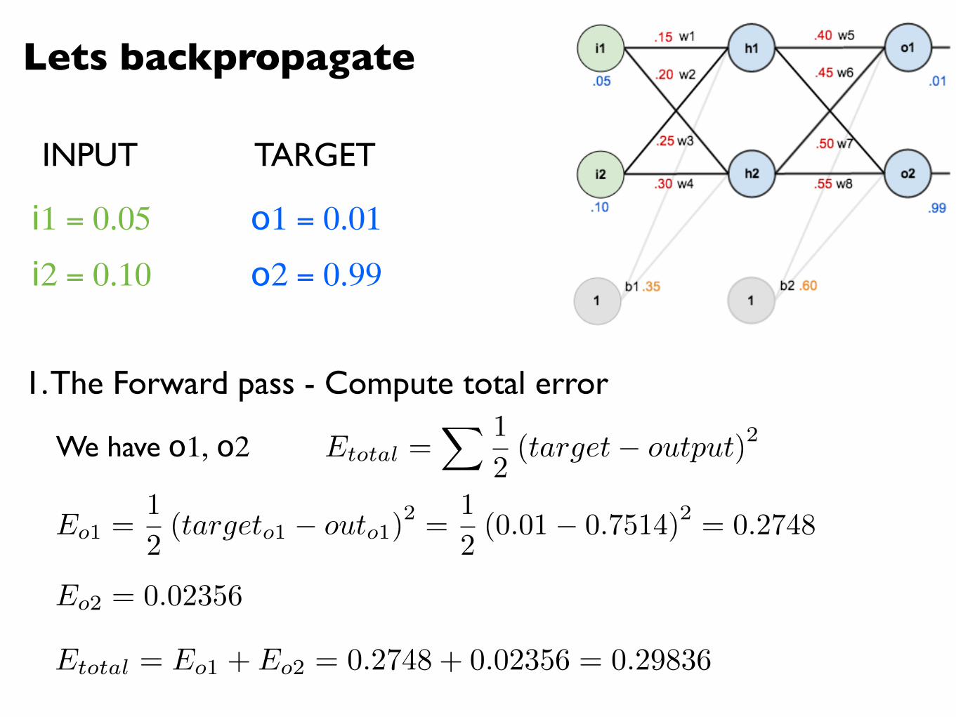
We have o1, o2 Etotal =X 1
2(target� output)2
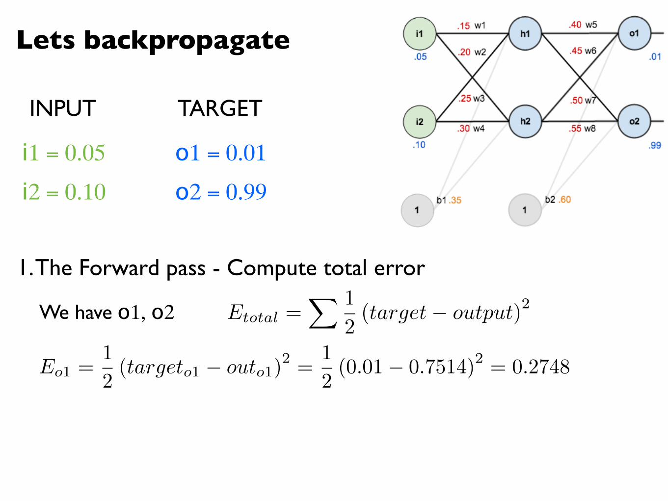
Lets backpropagate
i1 = 0.05
i2 = 0.10
o1 = 0.01
o2 = 0.99
1. The Forward pass - Compute total error
INPUT TARGET
We have o1, o2 Etotal =X 1
2(target� output)2
Eo1 =1
2(targeto1 � outo1)
2 =1
2(0.01� 0.7514)2 = 0.2748
Lets backpropagate
i1 = 0.05
i2 = 0.10
o1 = 0.01
o2 = 0.99
1. The Forward pass - Compute total error
INPUT TARGET
We have o1, o2 Etotal =X 1
2(target� output)2
Eo1 =1
2(targeto1 � outo1)
2 =1
2(0.01� 0.7514)2 = 0.2748
Eo2 = 0.02356
Lets backpropagate
i1 = 0.05
i2 = 0.10
o1 = 0.01
o2 = 0.99
1. The Forward pass - Compute total error
INPUT TARGET
We have o1, o2 Etotal =X 1
2(target� output)2
Eo1 =1
2(targeto1 � outo1)
2 =1
2(0.01� 0.7514)2 = 0.2748
Eo2 = 0.02356
Etotal = Eo1 + Eo2 = 0.2748 + 0.02356 = 0.29836
Lets backpropagate
i1 = 0.05
i2 = 0.10
o1 = 0.01
o2 = 0.99
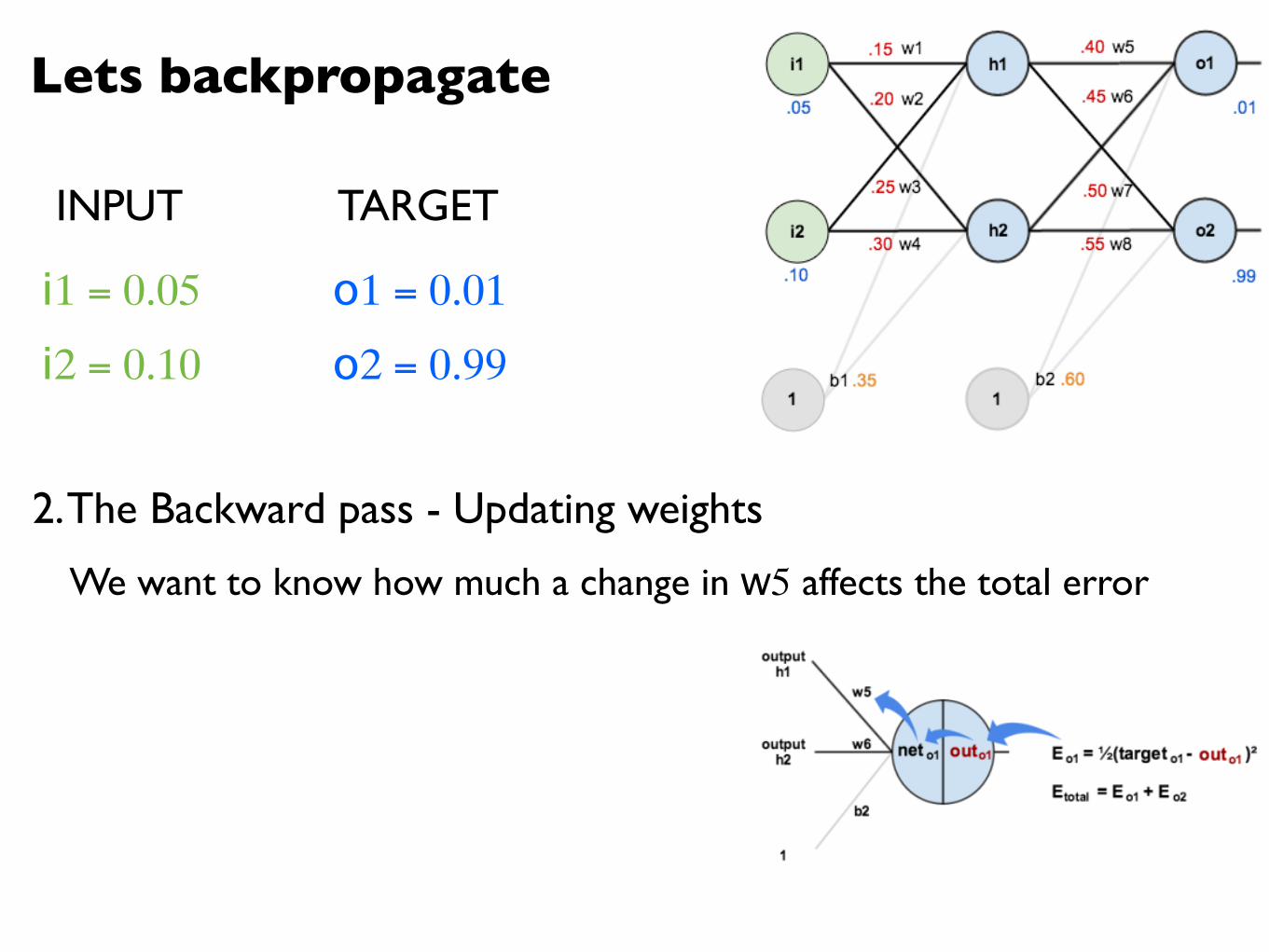
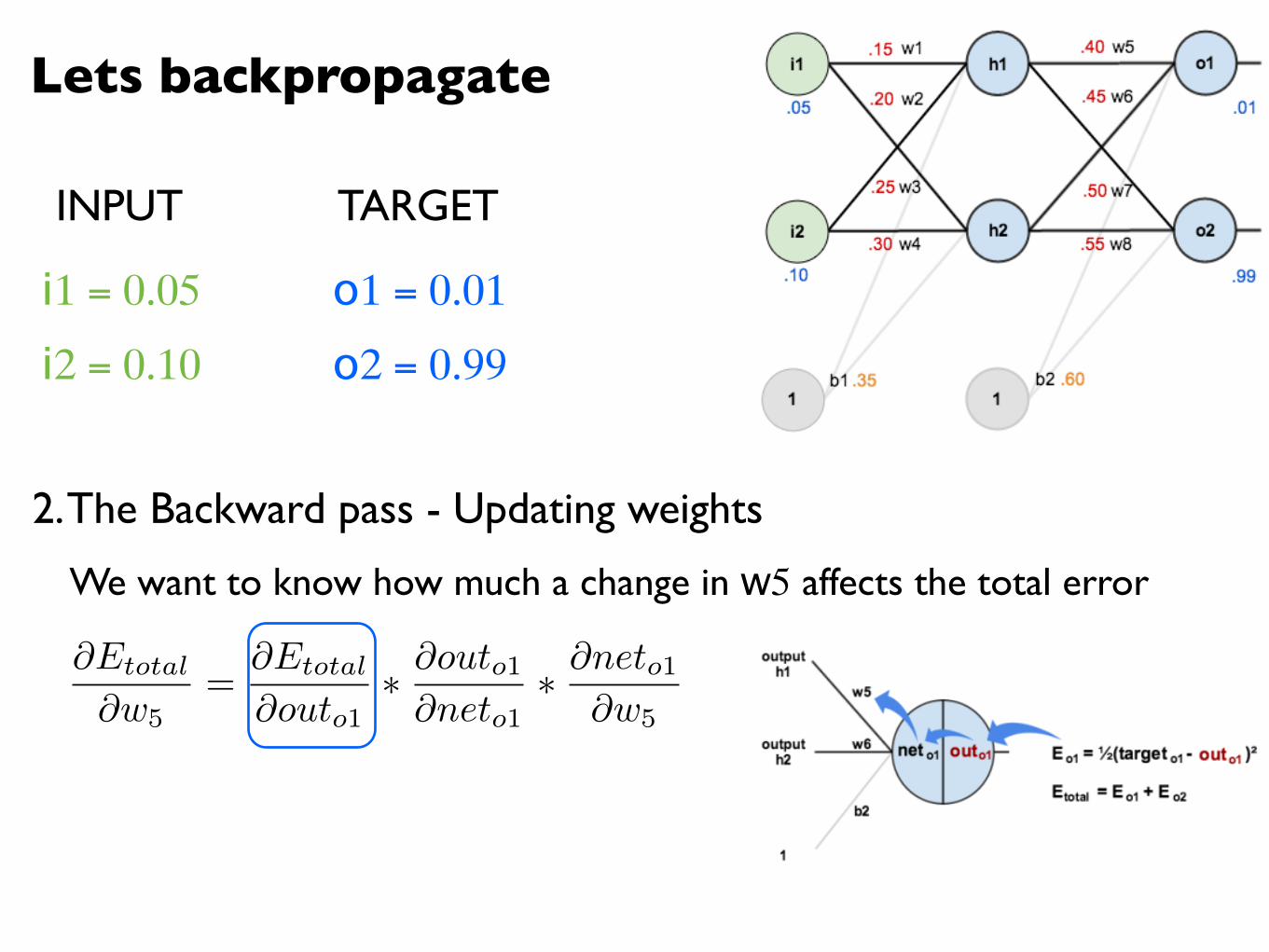
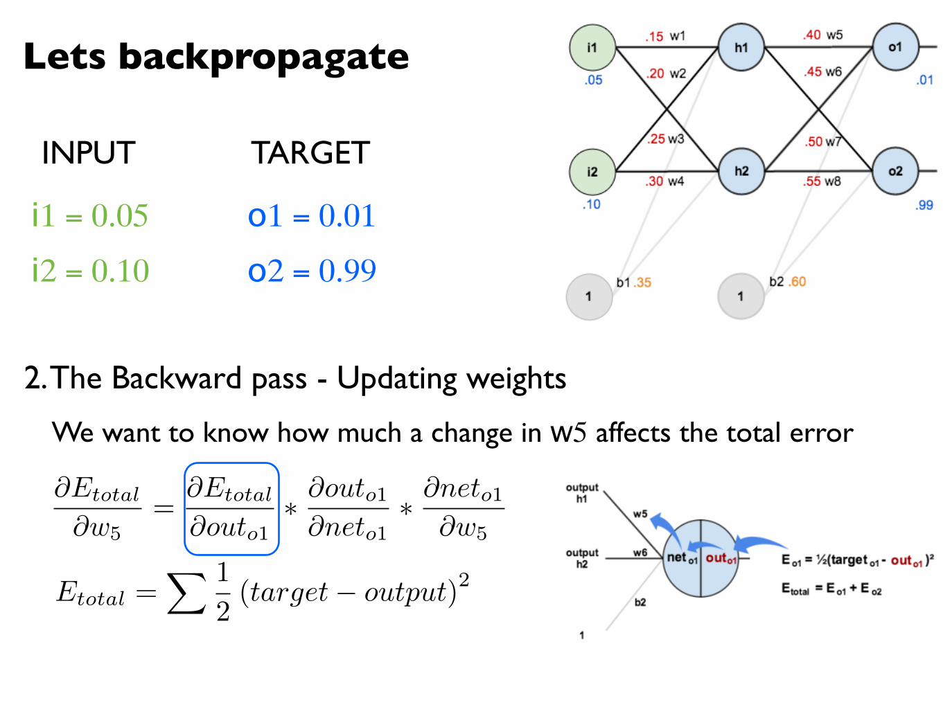
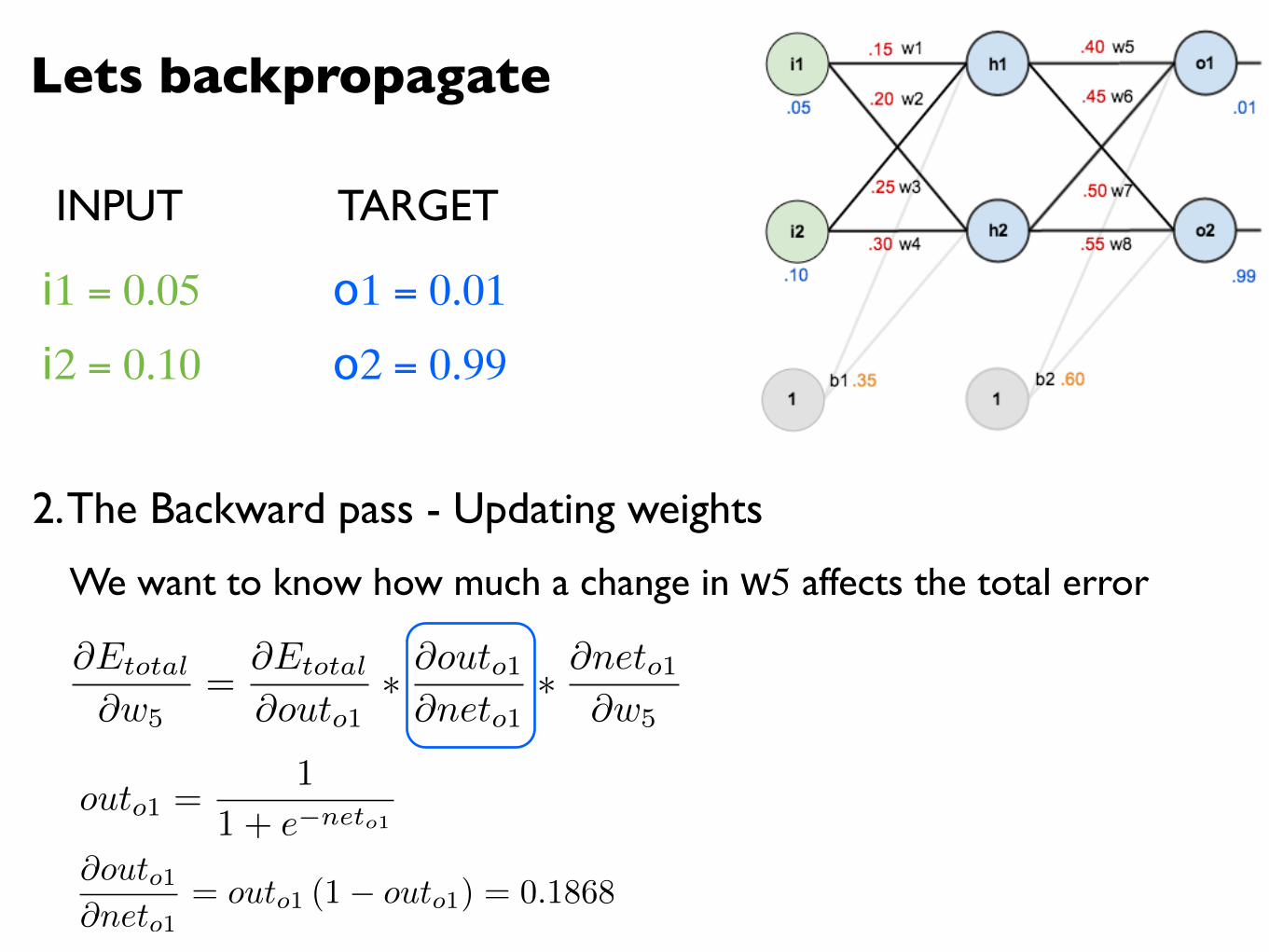
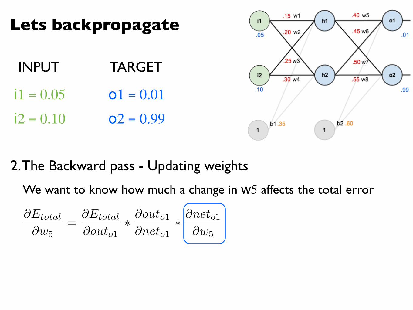
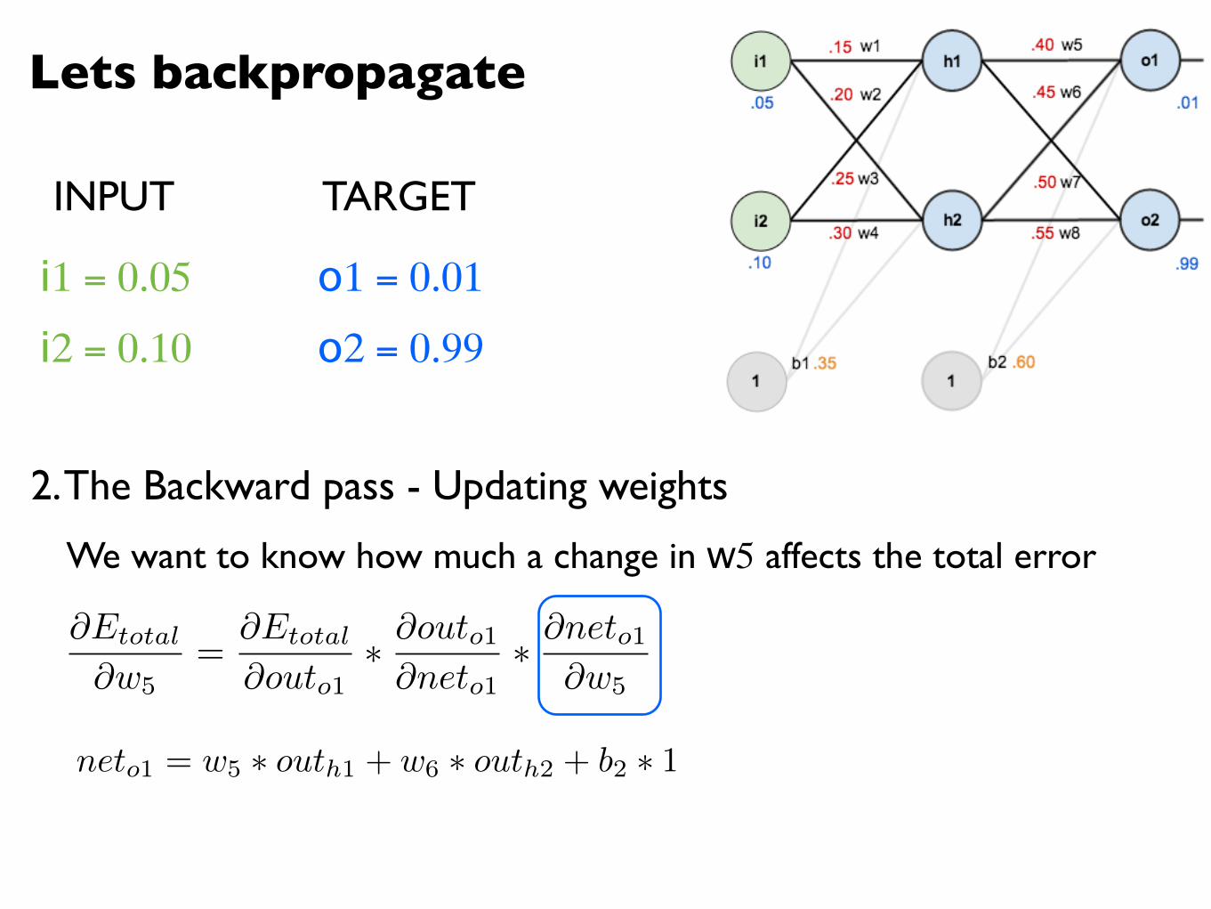
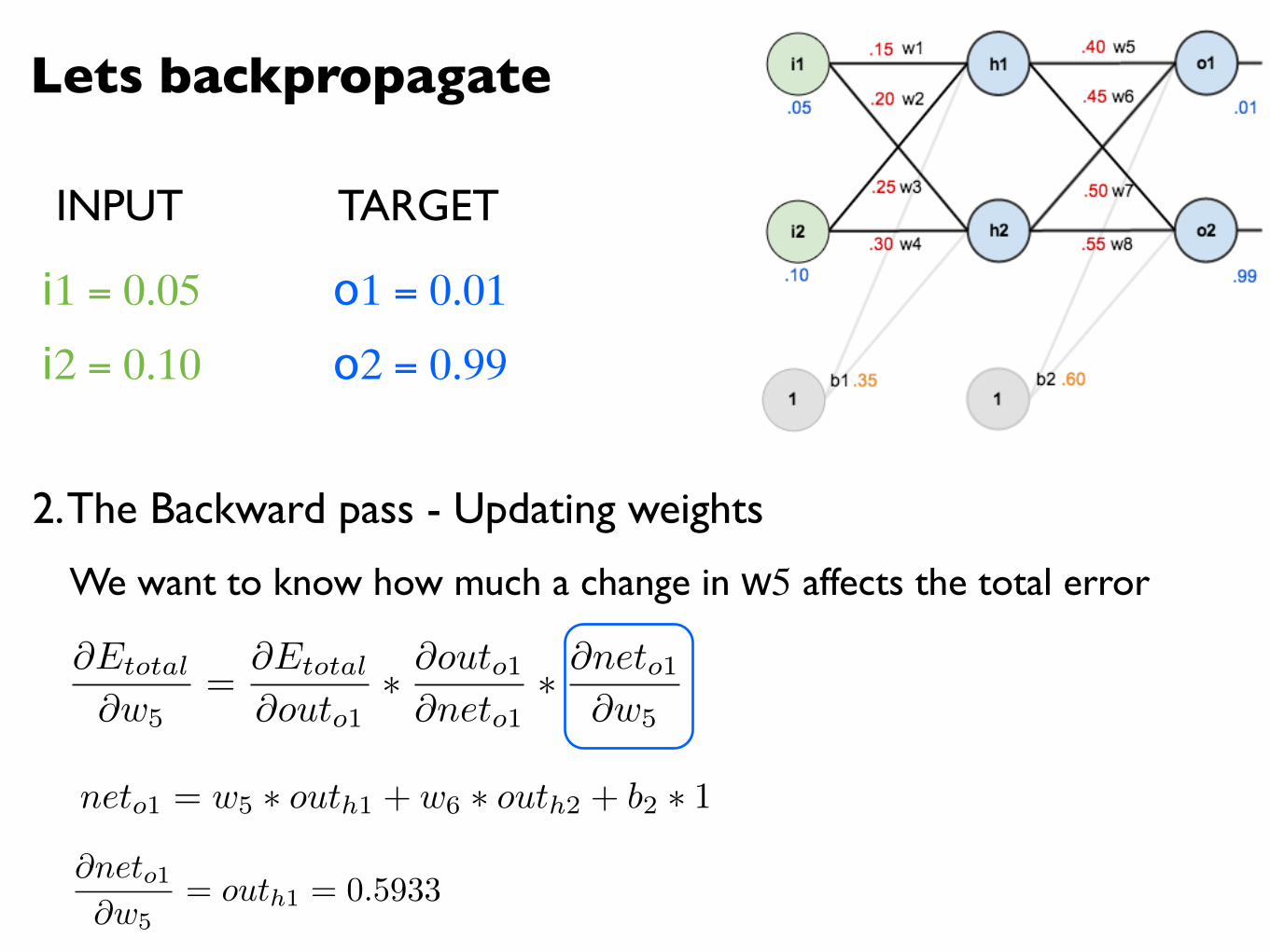
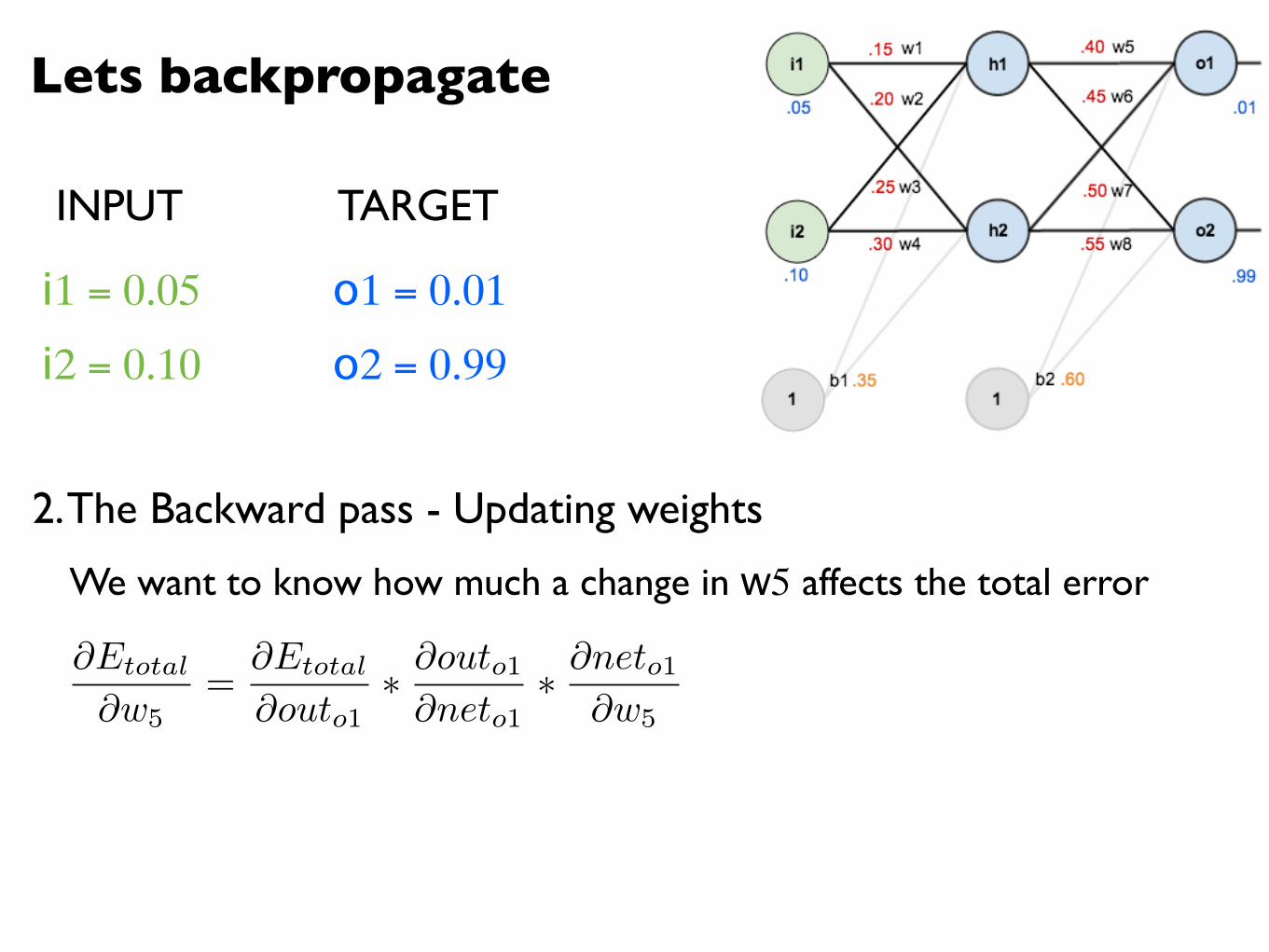
2. The Backward pass - Updating weights
INPUT TARGET
We want to know how much a change in w5 affects the total error

Lets backpropagate
i1 = 0.05
i2 = 0.10
o1 = 0.01
o2 = 0.99
2. The Backward pass - Updating weights
INPUT TARGET
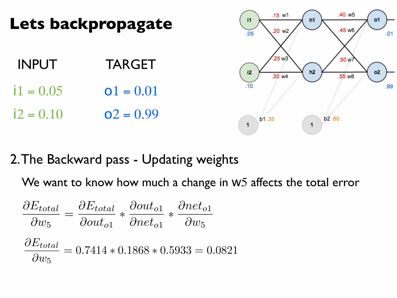
@Etotal
@w5=
@Etotal
@outo1⇤ @outo1@neto1
⇤ @neto1@w5
We want to know how much a change in w5 affects the total error
Lets backpropagate
i1 = 0.05
i2 = 0.10
o1 = 0.01
o2 = 0.99
2. The Backward pass - Updating weights
INPUT TARGET
@Etotal
@w5=
@Etotal
@outo1⇤ @outo1@neto1
⇤ @neto1@w5
We want to know how much a change in w5 affects the total error
Lets backpropagate
i1 = 0.05
i2 = 0.10
o1 = 0.01
o2 = 0.99
2. The Backward pass - Updating weights
INPUT TARGET
Etotal =X 1
2(target� output)2
@Etotal
@w5=
@Etotal
@outo1⇤ @outo1@neto1
⇤ @neto1@w5
We want to know how much a change in w5 affects the total error
Lets backpropagate
i1 = 0.05
i2 = 0.10
o1 = 0.01
o2 = 0.99
2. The Backward pass - Updating weights
INPUT TARGET
Etotal =X 1
2(target� output)2
@Etotal
@w5=
@Etotal
@outo1⇤ @outo1@neto1
⇤ @neto1@w5
We want to know how much a change in w5 affects the total error
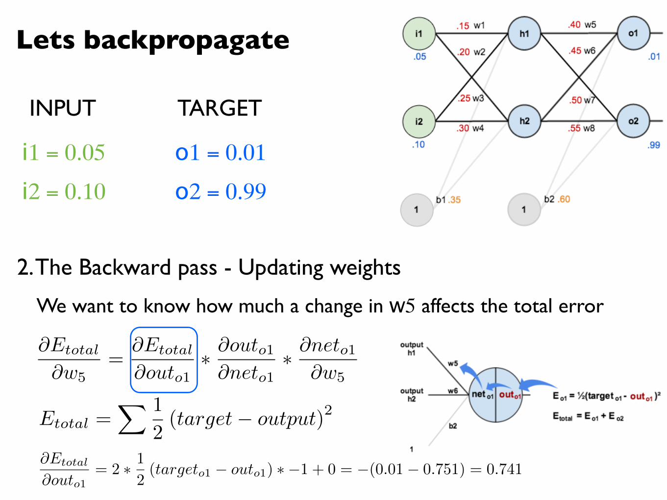
@Etotal
@outo1= 2 ⇤ 1
2(targeto1 � outo1) ⇤ �1 + 0 = �(0.01� 0.751) = 0.741
Lets backpropagate
i1 = 0.05
i2 = 0.10
o1 = 0.01
o2 = 0.99
2. The Backward pass - Updating weights
INPUT TARGET
@Etotal
@w5=
@Etotal
@outo1⇤ @outo1@neto1
⇤ @neto1@w5
We want to know how much a change in w5 affects the total error
Lets backpropagate
i1 = 0.05
i2 = 0.10
o1 = 0.01
o2 = 0.99
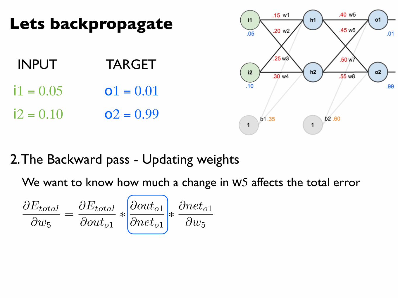
2. The Backward pass - Updating weights
INPUT TARGET
@Etotal
@w5=
@Etotal
@outo1⇤ @outo1@neto1
⇤ @neto1@w5
We want to know how much a change in w5 affects the total error
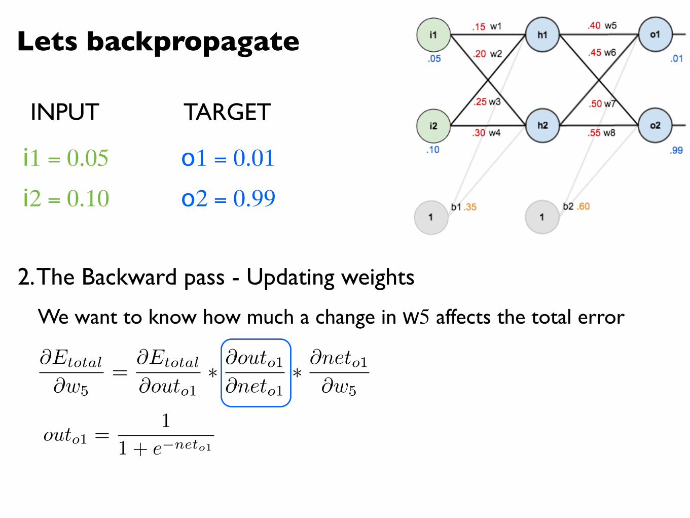
outo1 =1
1 + e�neto1
Lets backpropagate
i1 = 0.05
i2 = 0.10
o1 = 0.01
o2 = 0.99
2. The Backward pass - Updating weights
INPUT TARGET
@Etotal
@w5=
@Etotal
@outo1⇤ @outo1@neto1
⇤ @neto1@w5
We want to know how much a change in w5 affects the total error
@outo1@neto1
= outo1 (1� outo1) = 0.1868
outo1 =1
1 + e�neto1
Lets backpropagate
i1 = 0.05
i2 = 0.10
o1 = 0.01
o2 = 0.99
2. The Backward pass - Updating weights
INPUT TARGET
@Etotal
@w5=
@Etotal
@outo1⇤ @outo1@neto1
⇤ @neto1@w5
We want to know how much a change in w5 affects the total error
Lets backpropagate
i1 = 0.05
i2 = 0.10
o1 = 0.01
o2 = 0.99
2. The Backward pass - Updating weights
INPUT TARGET
@Etotal
@w5=
@Etotal
@outo1⇤ @outo1@neto1
⇤ @neto1@w5
We want to know how much a change in w5 affects the total error
neto1 = w5 ⇤ outh1 + w6 ⇤ outh2 + b2 ⇤ 1
Lets backpropagate
i1 = 0.05
i2 = 0.10
o1 = 0.01
o2 = 0.99
2. The Backward pass - Updating weights
INPUT TARGET
@Etotal
@w5=
@Etotal
@outo1⇤ @outo1@neto1
⇤ @neto1@w5
We want to know how much a change in w5 affects the total error
neto1 = w5 ⇤ outh1 + w6 ⇤ outh2 + b2 ⇤ 1
@neto1@w5
= outh1 = 0.5933
Lets backpropagate
i1 = 0.05
i2 = 0.10
o1 = 0.01
o2 = 0.99
2. The Backward pass - Updating weights
INPUT TARGET
@Etotal
@w5=
@Etotal
@outo1⇤ @outo1@neto1
⇤ @neto1@w5
We want to know how much a change in w5 affects the total error
Lets backpropagate
i1 = 0.05
i2 = 0.10
o1 = 0.01
o2 = 0.99
2. The Backward pass - Updating weights
INPUT TARGET
@Etotal
@w5=
@Etotal
@outo1⇤ @outo1@neto1
⇤ @neto1@w5
We want to know how much a change in w5 affects the total error
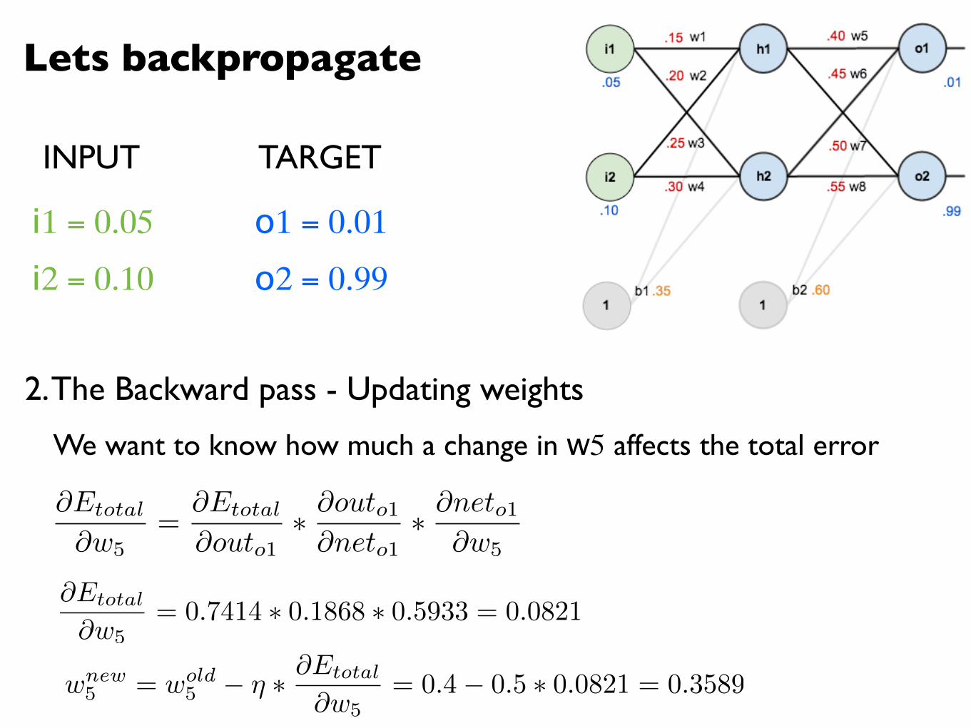
@Etotal
@w5= 0.7414 ⇤ 0.1868 ⇤ 0.5933 = 0.0821
Lets backpropagate
i1 = 0.05
i2 = 0.10
o1 = 0.01
o2 = 0.99
2. The Backward pass - Updating weights
INPUT TARGET
@Etotal
@w5=
@Etotal
@outo1⇤ @outo1@neto1
⇤ @neto1@w5
We want to know how much a change in w5 affects the total error
@Etotal
@w5= 0.7414 ⇤ 0.1868 ⇤ 0.5933 = 0.0821
wnew5 = wold
5 � ⌘ ⇤ @Etotal
@w5= 0.4� 0.5 ⇤ 0.0821 = 0.3589
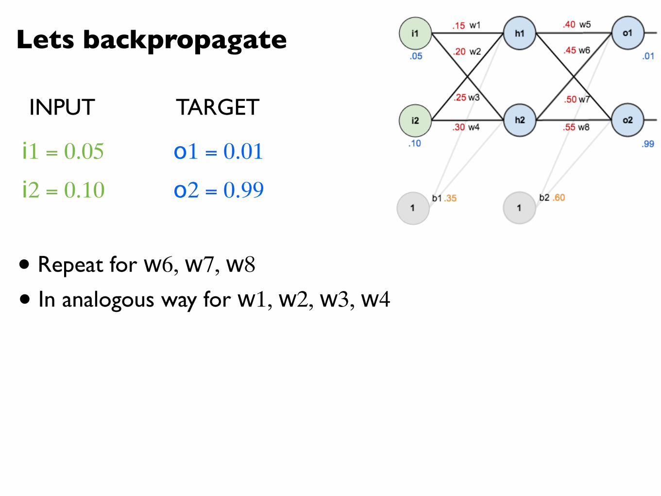
Lets backpropagate
i1 = 0.05
i2 = 0.10
o1 = 0.01
o2 = 0.99
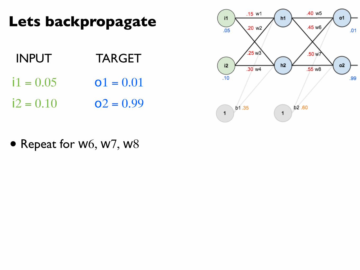
• Repeat for w6, w7, w8
INPUT TARGET
Lets backpropagate
i1 = 0.05
i2 = 0.10
o1 = 0.01
o2 = 0.99
• Repeat for w6, w7, w8
INPUT TARGET
• In analogous way for w1, w2, w3, w4
Lets backpropagate
i1 = 0.05
i2 = 0.10
o1 = 0.01
o2 = 0.99
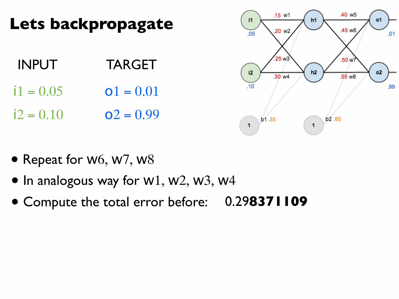
• Repeat for w6, w7, w8
INPUT TARGET
• In analogous way for w1, w2, w3, w4
• Compute the total error before: 0.298371109
Lets backpropagate
i1 = 0.05
i2 = 0.10
o1 = 0.01
o2 = 0.99
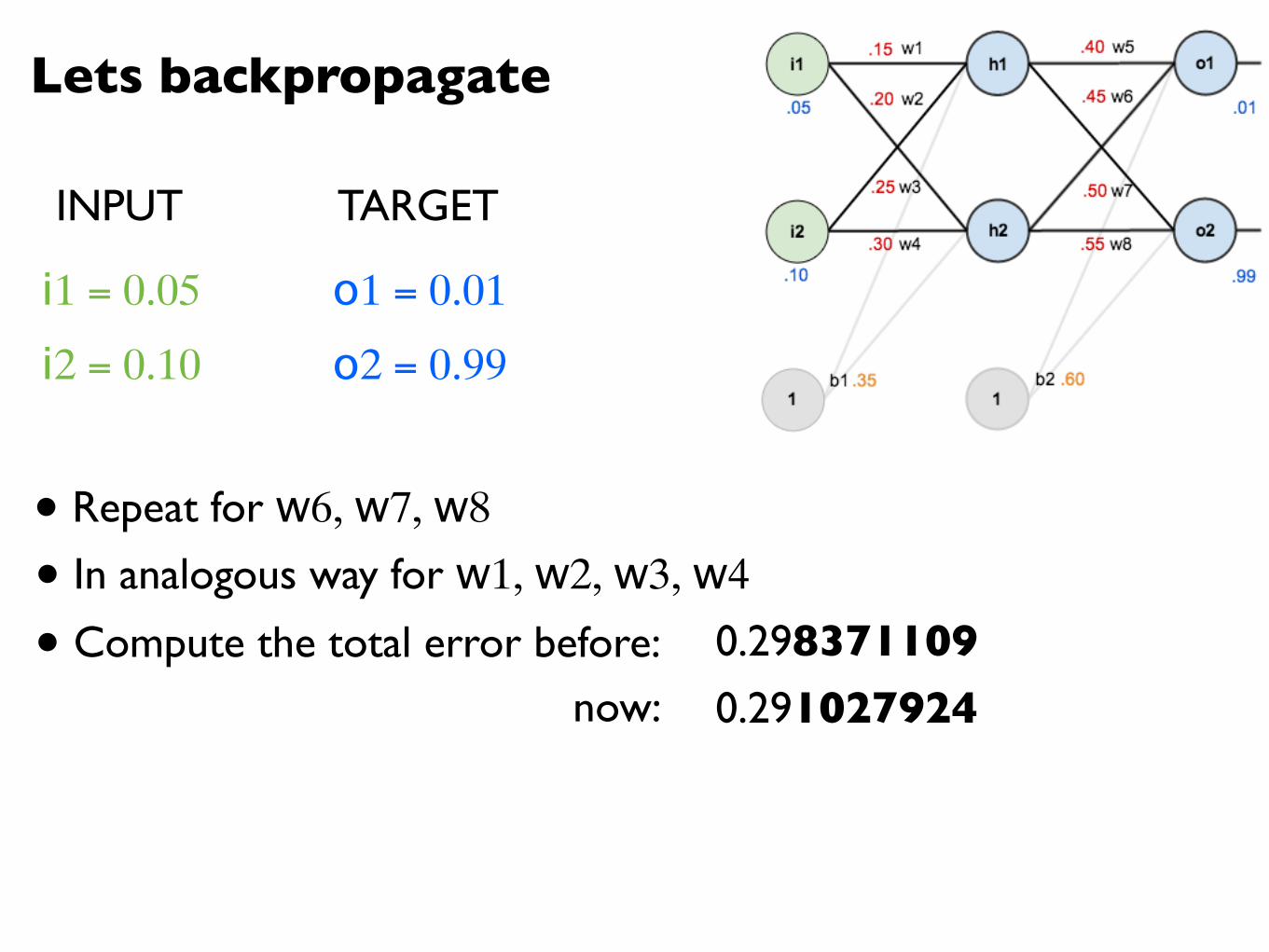
• Repeat for w6, w7, w8
INPUT TARGET
• In analogous way for w1, w2, w3, w4
• Compute the total error before:now:
0.2983711090.291027924
Lets backpropagate
i1 = 0.05
i2 = 0.10
o1 = 0.01
o2 = 0.99
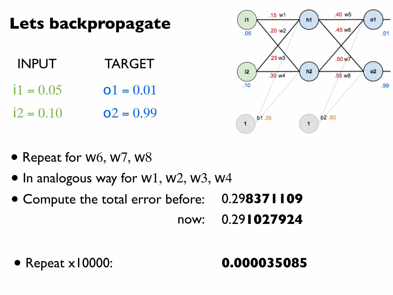
• Repeat for w6, w7, w8
INPUT TARGET
• In analogous way for w1, w2, w3, w4
• Compute the total error before:now:
0.2983711090.291027924
• Repeat x10000: 0.000035085
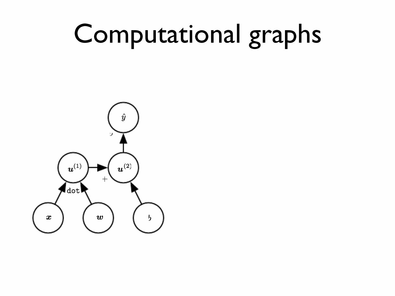
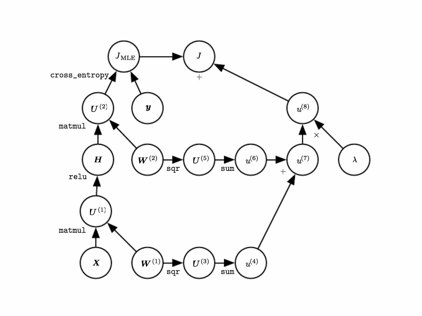
Computational graphs
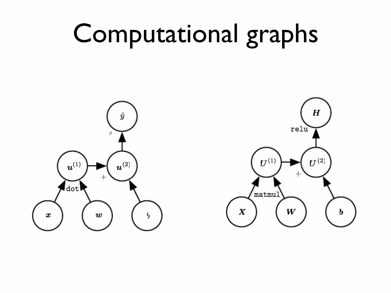
Computational graphs
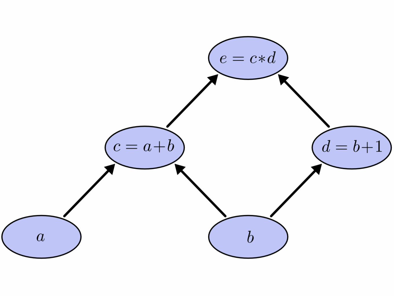

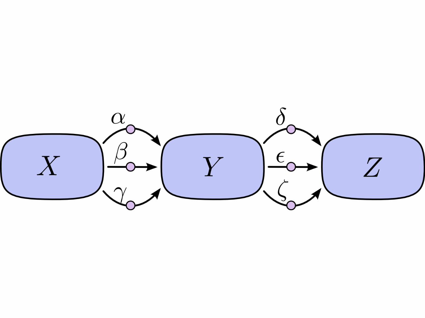
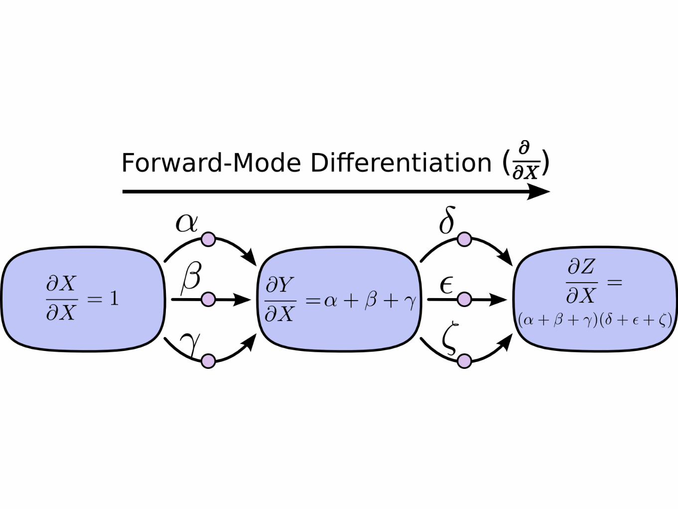
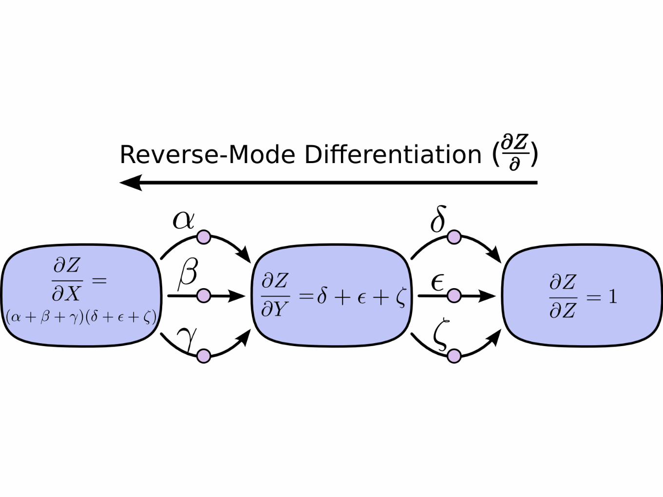

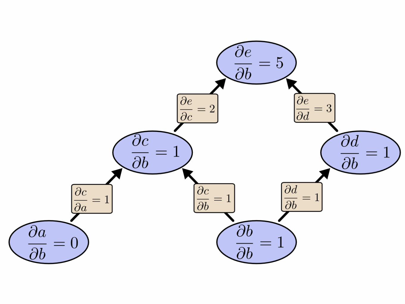
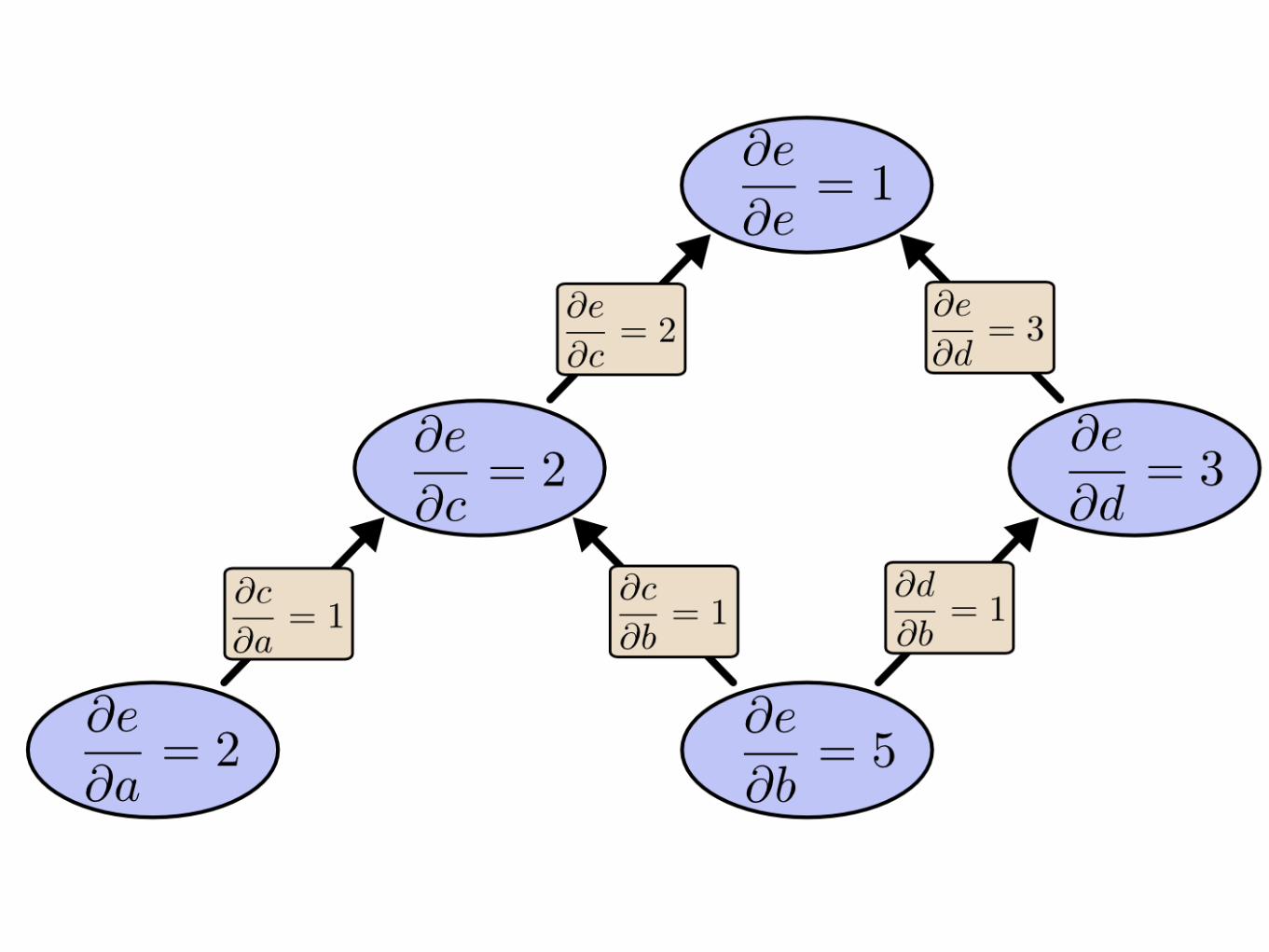
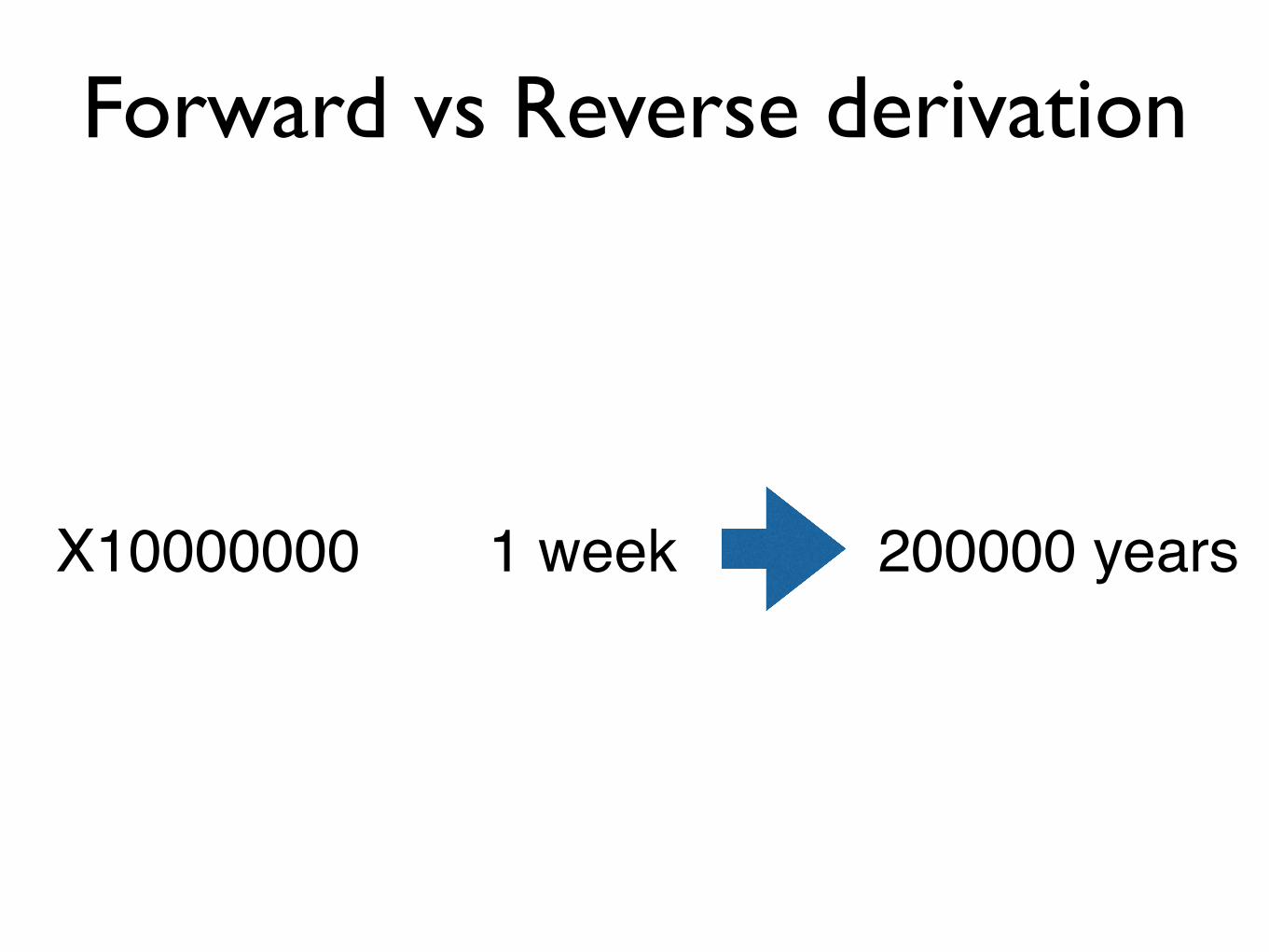
Forward vs Reverse derivation
X10000000 1 week 200000 years

Selected topics
Advanced
Basics
Foundations
Lesson Title
1 Introduction
2 Probability and Information Theory
3 Basics of Machine Learning
4 Deep Feed-forward networks
5 Back-propagation
6 Optimization and regularization
7 Convolutional Networks
8 Sequence Modeling: recurrent networks
9 Applications
10 Software and Practical methods
11 Autoencoders and GANs
12 Project Development
13 Deep Reinforcement Learning
14 Deep Learning and the Brain
15 Conclusions and Future Perspective
16 Project presentations