lecture 6 correlation and regression · correlation coefficient • the range of correlation...
TRANSCRIPT
Lecture 11
Correlation and
Regression

Overview of the Correlation
and Regression Analysis
The Correlation Analysis • In statistics, dependence refers to any statistical
relationship between two random variables or two sets of
data. Correlation refers to any of a broad class of
statistical relationships involving dependence.
• Familiar examples of dependent phenomena include the
correlation between the physical statures of parents and
their offspring, and the correlation between the demand
for a product and its price.
• Correlations are useful because they can indicate a
predictive relationship that can be exploited in practice.
– For example, an electrical utility may produce less power on a
mild day based on the correlation between electricity demand
and weather. In this example there is a causal relationship,
because extreme weather causes people to use more electricity
for heating or cooling; however, statistical dependence is not
sufficient to demonstrate the presence of such a causal
relationship (i.e., Correlation does not imply causation).
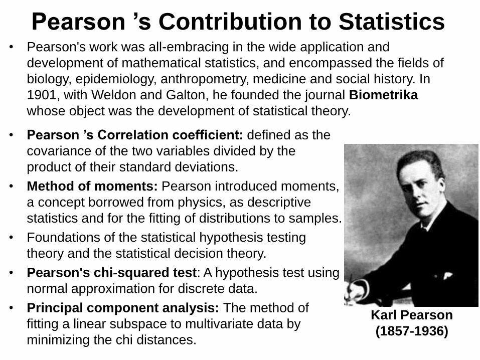
Pearson ’s Contribution to Statistics • Pearson's work was all-embracing in the wide application and
development of mathematical statistics, and encompassed the fields of
biology, epidemiology, anthropometry, medicine and social history. In
1901, with Weldon and Galton, he founded the journal Biometrika
whose object was the development of statistical theory.
Karl Pearson
(1857-1936)
• Pearson ’s Correlation coefficient: defined as the
covariance of the two variables divided by the
product of their standard deviations.
• Method of moments: Pearson introduced moments,
a concept borrowed from physics, as descriptive
statistics and for the fitting of distributions to samples.
• Foundations of the statistical hypothesis testing
theory and the statistical decision theory.
• Pearson's chi-squared test: A hypothesis test using
normal approximation for discrete data.
• Principal component analysis: The method of
fitting a linear subspace to multivariate data by
minimizing the chi distances.

The Regression Analysis
• In statistics, regression analysis is a statistical technique for
estimating the relationships among variables. It includes many
techniques for modeling and analyzing several variables, when
the focus is on the relationship between a dependent variable
and one or more independent variables.
• More specifically, regression analysis helps one understand how
the typical value of the dependent variable changes when any
one of the independent variables is varied, while the other
independent variables are held fixed.
• Regression analysis is widely used for prediction and
forecasting, where its use has substantial overlap with the field
of machine learning.
• Regression analysis is also used to understand which among
the independent variables are related to the dependent variable,
and to explore the forms of these relationships.
History of Regression • The earliest form of regression was the method of least squares,
which was published by Legendre in 1805, and by Gauss in 1809.
Gauss published a further development of the theory of least squares in
1821, including a version of the Gauss–Markov theorem.
• The term "regression" was coined by Francis Galton in the nineteenth
century to describe a biological phenomenon. The phenomenon was
that the heights of descendants of tall ancestors tend to regress down
towards a normal average (a phenomenon also known as regression
toward the mean
• In the 1950s and 1960s, economists used electromechanical desk
calculators to calculate regressions. Before 1970, it sometimes took up
to 24 hours to receive the result from one regression.
• Regression methods continue to be an area of active research. In recent decades, new
methods have been developed for robust regression, regression involving correlated
responses such as time series and growth curves, regression in which the predictor or
response variables are curves, images, graphs, or other complex data objects, regression
methods accommodating various types of missing data, nonparametric regression,
Bayesian methods for regression, regression in which the predictor variables are
measured with error, regression with more predictor variables than observations, and
causal inference with regression.
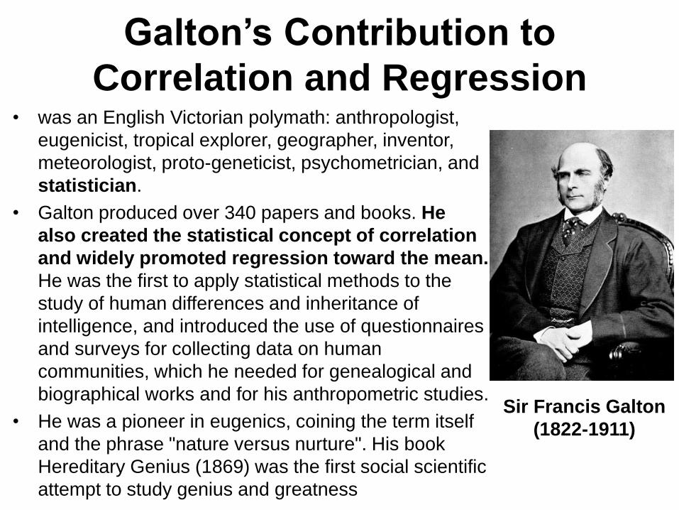
Galton’s Contribution to
Correlation and Regression • was an English Victorian polymath: anthropologist,
eugenicist, tropical explorer, geographer, inventor,
meteorologist, proto-geneticist, psychometrician, and
statistician.
• Galton produced over 340 papers and books. He
also created the statistical concept of correlation
and widely promoted regression toward the mean.
He was the first to apply statistical methods to the
study of human differences and inheritance of
intelligence, and introduced the use of questionnaires
and surveys for collecting data on human
communities, which he needed for genealogical and
biographical works and for his anthropometric studies.
• He was a pioneer in eugenics, coining the term itself
and the phrase "nature versus nurture". His book
Hereditary Genius (1869) was the first social scientific
attempt to study genius and greatness
Sir Francis Galton
(1822-1911)
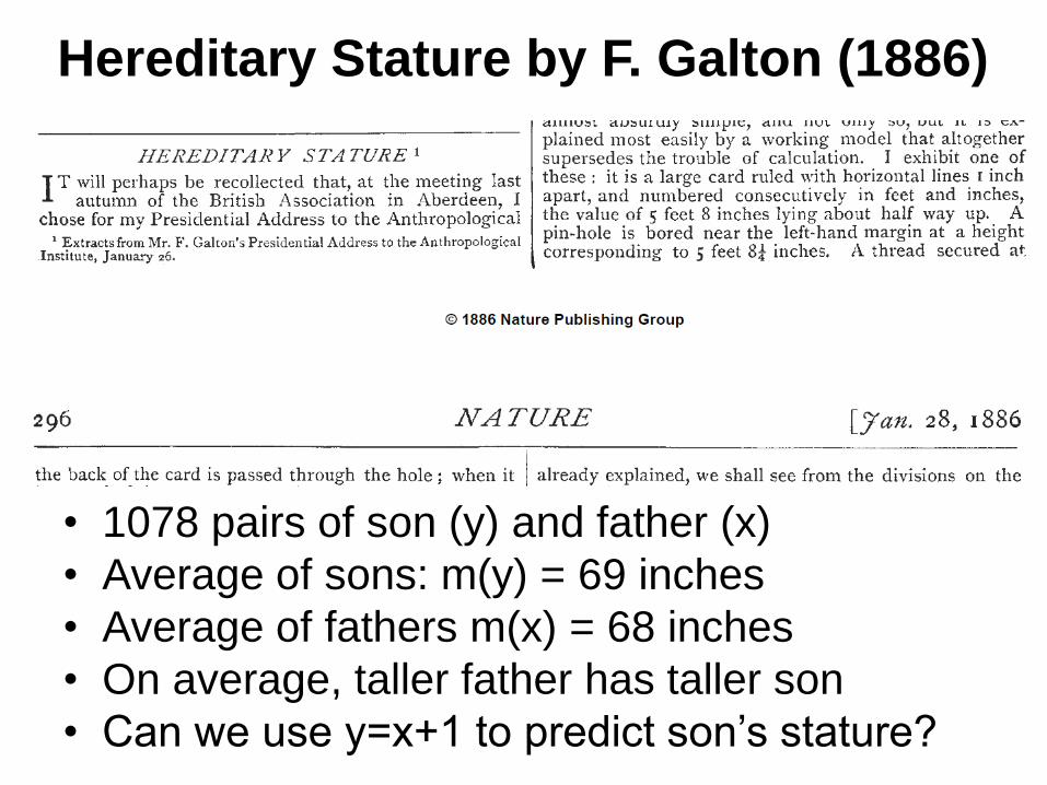
Hereditary Stature by F. Galton (1886)
• 1078 pairs of son (y) and father (x)
• Average of sons: m(y) = 69 inches
• Average of fathers m(x) = 68 inches
• On average, taller father has taller son
• Can we use y=x+1 to predict son’s stature?
64
65
66
67
68
69
70
71
72
73
64 65 66 67 68 69 70 71 72
Son
's h
eig
ht
(in
che
s)
Father's height (inches)
y=x+1
y=35+0.5x
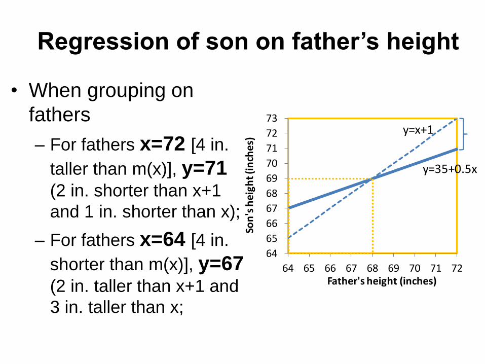
Regression of son on father’s height
• When grouping on
fathers
– For fathers x=72 [4 in.
taller than m(x)], y=71
(2 in. shorter than x+1
and 1 in. shorter than x);
– For fathers x=64 [4 in.
shorter than m(x)], y=67 (2 in. taller than x+1 and
3 in. taller than x;

Regression of offspring on
mid-parent height
• Slope from
offspring and
mid-parent is
higher than
slope from son
and father!

Galton’s explanation of regression
• Resemblance between offspring and
parents
• Regression
– The term "regression" was coined by Francis
Galton in the nineteenth century to describe
a biological phenomenon.
– The phenomenon was that the heights of
descendants of tall ancestors tend to
regress down towards a normal average (a
phenomenon also known as regression
toward the mean).

Correlation Analysis
Correlation analysis
• Correlation Analysis is the study of the
relationship between two variables.
• Scatter Plot
• Correlation Coefficient

Scatter plot
• A scatter plot is a graph of the
ordered pairs (X,Y) of numbers
consisting of the independent
variables X and the dependent
variables Y.
• It is usually the first step in
correlation analysis.

Scatter plot example
• The plot shows the relationship
between the grade and the hours
studied of a course of six students
The graph suggests a
positive relationship
between hours of
studies and grades
0 1 2 3 4 5 6
02
04
06
08
0
Scatter Plot
Hours studied
Gra
de

Correlation coefficient
• Measures the strength and direction of the
linear relationship between two variables X
and Y
• Population Correlation Coefficient:
• Sample Correlation Coefficient:
22
),(
EYYEEXXE
EYYEXXE
DYDX
YXCovXY
n
i
i
n
i
i
n
i
ii
yx
xy
YYn
XXn
YYXXn
ss
sr
1
2
1
2
1
22
2
1
1
1
1
1
1
Correlation coefficient
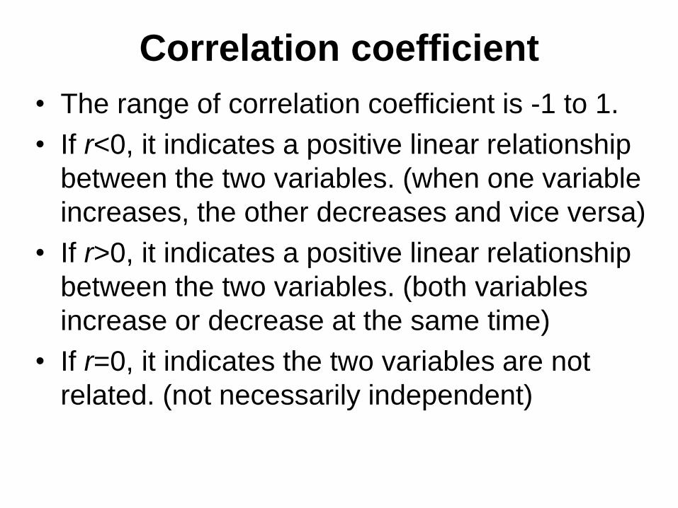
• The range of correlation coefficient is -1 to 1.
• If r<0, it indicates a positive linear relationship
between the two variables. (when one variable
increases, the other decreases and vice versa)
• If r>0, it indicates a positive linear relationship
between the two variables. (both variables
increase or decrease at the same time)
• If r=0, it indicates the two variables are not
related. (not necessarily independent)

Distribution of r
• The population correlation coefficient ρ is usually
not known. Therefore, the sample statistic r is
used to estimate ρ and to carry out tests of
hypotheses.
• If the true correlation between X and Y within the
general population is ρ=0, and if the size of the
sample , then
6n
)2(1
22
nt
r
nrt

Example
• The observations of two variables are
• Then r=-0.8371. H0: ρ=0
• So at a 99% confidence level, the null
hypothesis H0 of no relationship in the
population (ρ=0) is rejected.
X 35.5 34.1 31.7 40.3 36.8 40.2 31.7 39.2 44.2
y 12 16 9 2 7 3 13 9 -1
05.4)8371.0(--1
2-98371.0-
1
222
r
nrt
tt 499.3)7(01.0

Correlation coefficient
• From the example, we find that the t
statistic is a function of sample correlation
coefficient r, sample size n and confidence
level α.
• For any particular sample size, an
observed value of r is regarded as
statistically significant at the 95% level if
and only if its distance from zero is equal to
or greater than the distance of the tabled
value of r.

Correlation coefficient (95% level)
n ±r n ±r 6 0.73 19 0.39 7 0.67 20 0.38 8 0.62 21 0.37 9 0.58 22 0.36
10 0.55 23 0.35 11 0.52 24 0.34 12 0.5 25 0.34 13 0.48 26 0.33 14 0.46 27 0.32 15 0.44 28 0.32 16 0.43 29 0.31 17 0.41 30 0.31 18 0.4 31 0.3

Linear Regression Analysis

Linear regression
• Linear regression is used to study an
outcome as a linear function of one or
several predictors.
– xi: independent variables (predictors)
– y: dependent variable (effect)
• Regression analysis with one independent
variable is termed simple linear regression.
• Regression analysis with more than one
independent variables is termed multiple
linear regression.

Linear regression
• Given a data set {yi, xi1, …, xip} of n statistical
units, a linear regression model assumes that
the relationship between the dependent variable
yi and the p-vector of explanatory variables xi is
linear. This relationship is modeled through a
disturbance term or error variable εi. Thus the
model takes the form
nixxxy iippiii ,,2,1,2211

Linear regression
• Often these n equations are stacked together
and written in vector form as
Where εXβy
npnpn
p
p
nxx
xx
xx
y
y
y
2
1
1
0
1
221
111
2
1
,,
1
1
1
, εβXy

Linear regression
• yi is called the response variable or dependent
variable
• xi are called explanatory variables, predictor
variables, or independent variables. The matrix
is sometimes called the design matrix.
• β is a (p+1)-dimensional parameter vector. Its
elements are also called effects, or regression
coefficients. β0 is called intercept.
• ε is called the error term. This variable captures
all other factors which influence the dependent
variable yi other than the regressors xi.
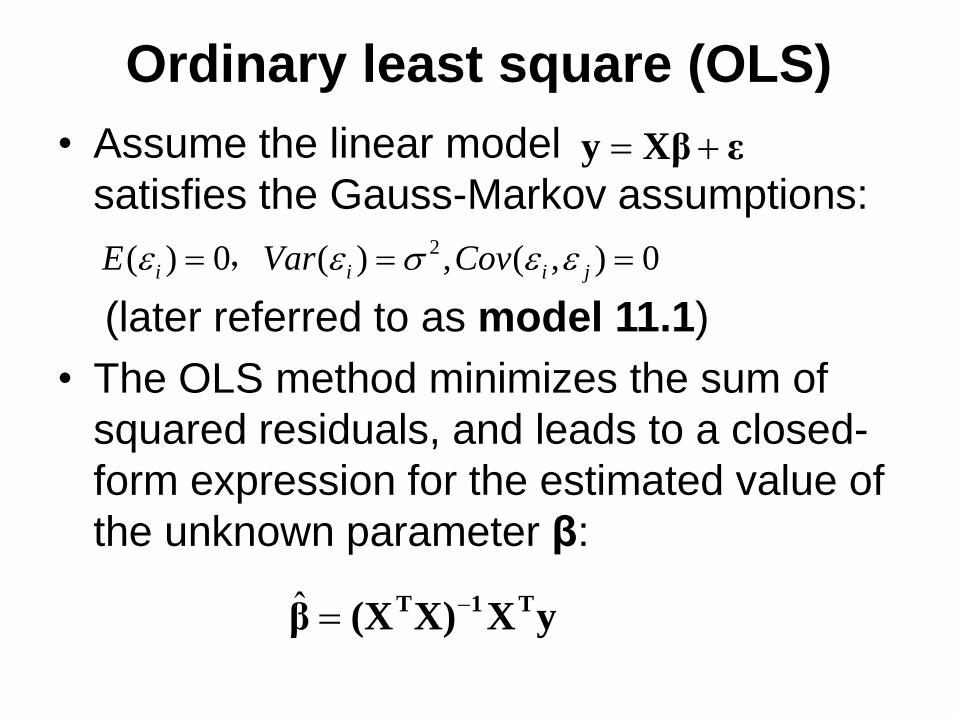
Ordinary least square (OLS)
• Assume the linear model
satisfies the Gauss-Markov assumptions:
(later referred to as model 11.1)
• The OLS method minimizes the sum of
squared residuals, and leads to a closed-
form expression for the estimated value of
the unknown parameter β:
εXβy
0),(,)(0)( 2 jiii CovVarE ,
yXX)(XβT1T ˆ
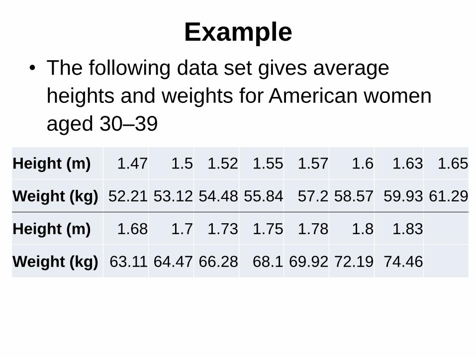
Example
• The following data set gives average
heights and weights for American women
aged 30–39
Height (m) 1.47 1.5 1.52 1.55 1.57 1.6 1.63 1.65
Weight (kg) 52.21 53.12 54.48 55.84 57.2 58.57 59.93 61.29
Height (m) 1.68 1.7 1.73 1.75 1.78 1.8 1.83
Weight (kg) 63.11 64.47 66.28 68.1 69.92 72.19 74.46

Scatter plot
1.50 1.55 1.60 1.65 1.70 1.75 1.80
55
60
65
70
75
Height(m)
Weig
ht(
kh)

Example
• The scatter plot suggests that the
relationship is strong and can be
approximated as a quadratic function.
• OLS can handle non-linear relationships
by introducing the regressor HEIGHT2.
The regression model then becomes a
multiple linear model:
iiii hhw 2
321

Example
• In matrix form:
Where
• The OLS estimator of is
• The relationship between weight and
height is
εHβw
15
2
1
2
1
0
2
1515
2
22
2
11
15
2
1
,,
1
1
1
,
εβHw
hh
hh
hh
w
w
w
β
TTT )9603.61,1620.143,8128.128(ˆ 1
wHHHβ
2*9603.61*1620.1438128.128 hhw

Properties of OLS estimators
• For model 11.1, the Least Square Estimator
has the following properties:
1.
2.
3. (Gauss-Markov Theorem) Among any unbiased
estimator of , has the minimum variance.
yXXXβTT 1)(ˆ
ββ ˆE
12ˆ XXβ
TCov
βcT
βc ˆT

Properties of OLS estimators
1.
2.
• Here is called residual
sum of squares. Its value reflects the
fitness of the regression model.
yXXXXIyTTTSS
1
1ˆ 2
pn
SS
n
i
ii
T yySS1
2ˆˆˆ

Centering and scaling
• In application, centering and scaling of
data matrix brings convenience.
• Centering:
pnpn
pp
pp
C
xxxx
xxxx
xxxx
11
2121
1111
X

Centering and scaling
• Scaling:
where ,
• Since Z is centered and scaled, it satisfies:
where
pnijz
Z
j
jij
ijs
xxz
n
i
jijj xxs1
22
0Z1 T
n ppij
T r
ZZR
ji
n
k
jkjiki
ijss
xxxx
r
1

Centering and scaling
• R is called the correlation matrix of design matrix
X. rij is the correlation coefficient between the ith
and jth column of X.
• The centered and scaled model takes the form
• Correspondingly, the OLS estimator of the
unknown parameter is
εZβ1y n
ZyZZβ
y1ˆ
ˆT

Centering and scaling
• When we have estimated values of intercept and
regression parameters (α and
respectively) in a centered and scaled model,
we can put the regression equation as
Tp ˆ,,ˆˆ1 β
p
i
i
i
p
i
i
i
i
p
p
pp
Xss
x
s
xX
s
xXY
11
1
1
11
ˆˆˆ
ˆˆˆ

Multicollinearity

Multicollinearity • Multicollinearity occurs when there is a
linear relationship among several
independent variables.
• In the case where we have two
independent variables, X1 and X2,
multicollinearity occurs when
X1i=a+bX2i,where a and b are constants.
• Intuitively, a problem arises because the
inclusion of both X1 and X2 adds no more
information to the model than the inclusion
of just one of them.

Multicollinearity • For model
the variance of, say, β1 is
where r12 is the correlation efficient between X1 and X2.
• If X1 and X2 are linearly related, then , and the
denominator goes to zero(in the limit), and the
variance goes to infinity, which means the estimator is
very unstable.
niXXY iiii ,,2,1,22110
2
12
2
1
2
2
12
2
11
2
111 rXrXX
Varii
12
12 r

Perfect & near-perfect
multicollinearity • What we have been discussing so far is really
perfect multicollinearity.
• Sometimes people use the term multicollinearity
to describe situations where there is a nearly
perfect linear relationship between the
independent variables.
• The assumptions of the linear regression model
only require that there be no perfect
multicollinearity. However, in practice, we almost
never face perfect multicollinearity but often
encounter near-perfect multicollinearity.

Perfect & near-perfect
multicollinearity
• Although the standard errors are technically
“correct” and will have minimum variance
with near perfect multicollinearity, they will
be very, very large.
• The intuition is, again, that the independent
variables are not providing much
independent information in the model and so
out coefficients are not estimated with a lot
of certainty.

Detection of multicollinearity
1. Variance Inflation Factor (VIF)
where is the coefficient of determination
of a regression of jth independent variable
on all the independent variables.
As a rule of thumb, VIF > 10 indicates high
multicollinearity.
21
1
jRVIF
2
jR

Detection of multicollinearity
2. Condition Number (k)
where and are the maximum and
minimum eigenvalue of the coefficient matrix
of design matrix respectively.
• As a rule of thumb, k>30 indicates high
multicollinearity.
m
k
1
1 m

Remedies for multicollinearity
1. Make sure you have not fallen into the
dummy variable trap; including a dummy
variable for every category (e.g., summer,
autumn, winter, and spring) and including
a constant term in the regression together
guarantee perfect multicollinearity.
2. Obtain more data, if possible. This is the
preferred solution.

Remedies for multicollinearity
3. Standardize your independent variables.
This may help reduce a false flagging of a
condition index above 30.
4. Apply a ridge regression or principal
component regression.
5. Select a subset of the independent
variable(which will be discussed later)

Hypothesis Tests

Hypothesis tests for a single
coefficient
• Consider normal linear regression model
Where
• Suppose that you want to test the hypothesis
that the true coefficient βj takes on some specific
value, βj,0. The null hypothesis and the two-sided
alternative hypothesis are
εXβy
),0( ~ i.i.d. 2 Ni
0,10,0 : vs.: jjjj HH
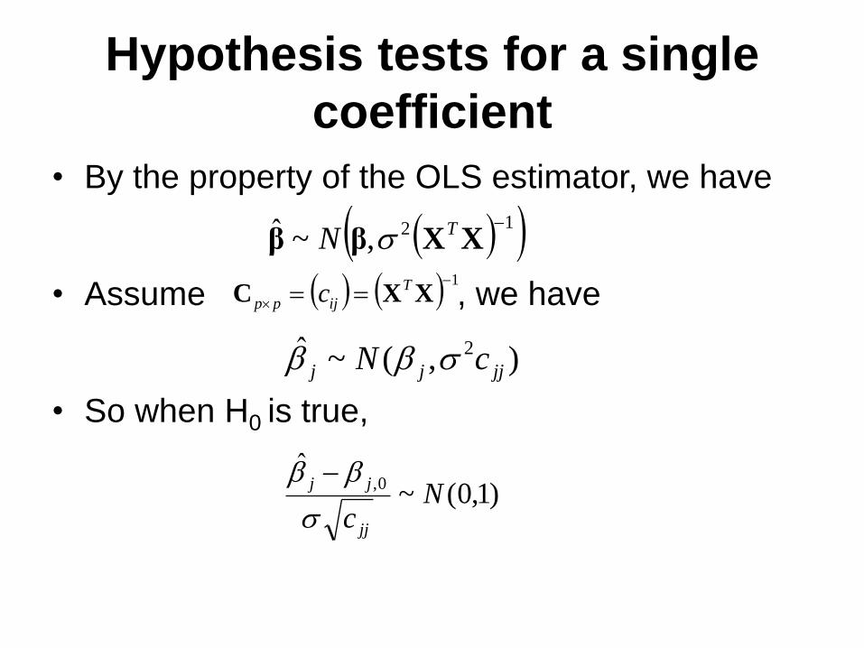
Hypothesis tests for a single
coefficient
• By the property of the OLS estimator, we have
• Assume , we have
• So when H0 is true,
12,~ˆ XXββ
TN
1
XXCT
ijpp c
),(~ˆ 2
jjjj cN
)1,0(~ˆ
0,N
c jj
jj

Hypothesis tests for a single
coefficient • Since in normal linear regression model there exists
and independent of , we have
where .
• With a given confidence level α, when
we can refuse the null hypothesis H0, otherwise
cannot.
2
12~ pn
SS
β
1
0,~
ˆ
ˆ
pn
jj
jj
j tc
t
1ˆ 2
pn
SS
21
pnj tt

Hypothesis tests for a single
coefficient
• If the regression model is not normal. By the
property of the OLS estimator, we have
• So under H0, the t statistic
where is the standard error of .
2ˆ,0ˆ
j
Nn jj
1,0
ˆ
ˆ0,
NSE
tj
jj
j
jSE j

Hypothesis tests for the model
• Consider normal linear regression model
Where
• To test hypothesis H0 on the model: β=0
εXβy
)N(0,~i.i.d. 2 i
1-,-1
2
nfyySS T
n
i
itot
pfyySS M
n
i
ireg
,-ˆ1
2
1,ˆ-1
2
pnfyySS M
n
i
iierr

Hypothesis tests for the model
• Under H0,
)1,1(~
1
pnF
pnSS
pSSF
err
reg
Source D.F. SS MS F
Model p SSreg MSreg=SSreg/p MSreg/MSerr
Error n-p-1 SSerr MSerr=SSerr/(n-p-1)
Total n-1 SStot

Example
• We also use this data:
X 35.5 34.1 31.7 40.3 36.8 40.2 31.7 39.2 44.2
y 12 16 9 2 7 3 13 9 -1
2.441
2.391
7.311
2.401
8.361
3.401
7.311
1.341
5.351
X
TTT )0996.1,5485.48(ˆ 1
yXXXβ
xy 0996.15493.48
0069.0256.0-
256.0-616.91XX
T

Calculation of SS 78.7y
Observation Prediction y Error
12 9.5135 2.4865
16 11.0529 4.9471
9 13.6920 -4.6920
2 4.2354 -2.2354
7 8.0840 -1.0840
3 4.3454 -1.3454
13 13.6920 -0.6920
9 5.4450 3.5550
-1 -0.0530 -0.9470
SSTot=249.5556, SSreg=174.9935, SSerr=74.6679
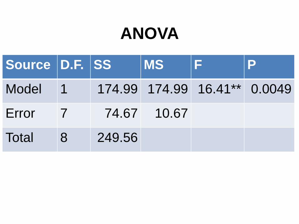
ANOVA
Source D.F. SS MS F P
Model 1 174.99 174.99 16.41** 0.0049
Error 7 74.67 10.67
Total 8 249.56

Test for coefficient
• H0: β=0
• So C11=0.007. Under H0,
• , so we reject H0.
7~05.4-0069.06668.10
0996.1-
ˆ
ˆt
ct
jj
6668.101
ˆ 2
pn
SS
0069.0256.0-
256.0-616.91XXC
T
ijpp c
2 0.05, When 1
pntt

Model Selection in
Regression
Model selection
• Model selection consists of two aspects:
1) linear or non- linear?
2) which variables to include?
• In this course, we only focus on the second
part, the variable selection in linear
regression.
• There are often
1) too many variables to choose from
2) different cost, different power
3) not an unequivocal “best”

Opposing criteria
• Good fit, good in-sample prediction:
– Make R2 large or MSE small
– Include many variables
• Parsimony:
– Keep cost of data collection low,
interpretation simple, standard errors
small
– Include few variables

Model selection criteria:
Coefficient of determination R2
• Definitions:
where
• In regression, the R2 is a statistical measure of how well the regression line approximates the real data points. An R2 closer to 1 indicates a better fit.
• Adding predictors(independent variables) always increase R2.
tot
err
tot
reg
SS
SS
SS
SSR 12
n
i
iierr
n
i
itot
n
i
ireg
yySS
yySSyySS
1
2
1
2
1
2
ˆ
,ˆ

Example
• In previous example:
– SSTot=249.5556
– SSreg=174.9935
– SSerr=74.6679
7012.05556.249
9935.1742 tot
reg
SS
SSR
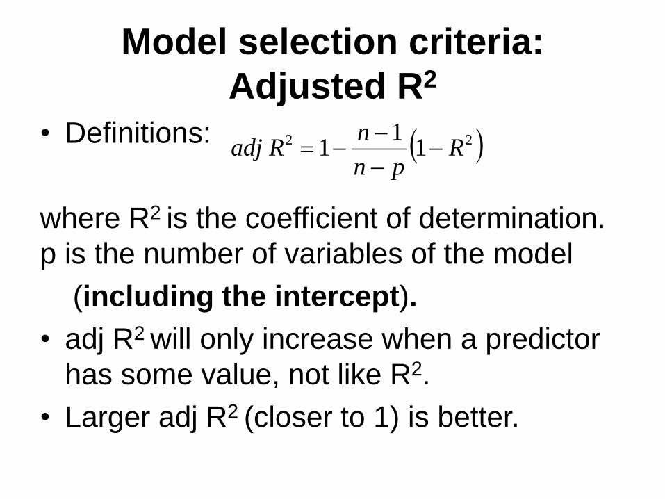
Model selection criteria:
Adjusted R2
• Definitions:
where R2 is the coefficient of determination.
p is the number of variables of the model
(including the intercept).
• adj R2 will only increase when a predictor
has some value, not like R2.
• Larger adj R2 (closer to 1) is better.
22 11
1 Rpn
nRadj

Model selection criteria:
AIC and BIC
• Definition:
AIC = −2(maximized log-likelihood) + 2p
BIC = -2(maximized log-likelihood) + p log(n)
• For linear regression,
-2(maximized log-likelihood) = n log(SSerr) + C
• Smaller value of AIC or BIC is better
• Get a balance between model fit and model size:
BIC penalizes larger models more heavily than
AIC ⇒ BIC tends to prefer smaller models

Model selection criteria:
Mallow's Cp
• Definition:
where estimated from the full model and
SSerr is obtained from a sub-model of interest.
• Cheap to compute
• Closely related to adj R2 and AIC, BIC.
• Performs well in predicting.
npSS
Cfull
errp
2
2ˆfull

Variable selection methods:
Best subsets selection
• Fit all possible models (all of the
various combinations of explanatory
variables) and evaluate which fits the
data best based on the criteria
above(except for R2 ).
• Usually takes a long time when
dealing with models with many
explanatory variables.

Variable selection methods:
Forward selection
• Starting with no variables in the model,
testing the addition of each variable
using a chosen model comparison
criterion, adding the variable (if any)
that improves the model the most, and
repeating this process until none
improves the model.

Variable selection methods:
Backward selection
• Starting with all candidate variables,
testing the deletion of each variable
using a chosen model comparison
criterion, deleting the variable (if any)
that improves the model the most by
being deleted, and repeating this
process until no further improvement
is possible.

Variable selection methods:
Stepwise selection
• A combination of the forward
selection and the backward selection,
testing at each step for variables to
be included or excluded.

Model selection example
• We will model a multiple linear regression for a
dataset (Longley's Economic Regression Data)
through different model selection approaches
and criteria.
• The dataset shows the relationship between the
dependent variable GNP deflator and the
possible predictor variables.
• The objective is to find out the a subset of all the
predictor variables which truly have an
significant effect on the dependent variable and
to evaluate the effect.

GNP deflator and the possible predictor variables
GNP
Deflator GNP Unemployed
Armed
Forces Population Year Employed
1947 83 234.289 235.6 159 107.608 1947 60.323 1948 88.5 259.426 232.5 145.6 108.632 1948 61.122 1949 88.2 258.054 368.2 161.6 109.773 1949 60.171 1950 89.5 284.599 335.1 165 110.929 1950 61.187 1951 96.2 328.975 209.9 309.9 112.075 1951 63.221 1952 98.1 346.999 193.2 359.4 113.27 1952 63.639 1953 99 365.385 187 354.7 115.094 1953 64.989 1954 100 363.112 357.8 335 116.219 1954 63.761 1955 101.2 397.469 290.4 304.8 117.388 1955 66.019 1956 104.6 419.18 282.2 285.7 118.734 1956 67.857 1957 108.4 442.769 293.6 279.8 120.445 1957 68.169 1958 110.8 444.546 468.1 263.7 121.95 1958 66.513 1959 112.6 482.704 381.3 255.2 123.366 1959 68.655 1960 114.2 502.601 393.1 251.4 125.368 1960 69.564 1961 115.7 518.173 480.6 257.2 127.852 1961 69.331 1962 116.9 554.894 400.7 282.7 130.081 1962 70.551

Full model
Estimate and significance test
of regression parameters Estimate Std.Error t value Pr(>|t|)
(intercept) 2946.85636 5647.97658 0.522 0.6144
GNP 0.26353 0.10815 2.437 0.0376
Unemployed 0.03648 0.03024 1.206 0.2585
Armed Forces 0.1116 0.01545 0.722 0.4885
Population -1.73703 0.67382 -2.578 0.0298
Year -1.4188 2.9446 -0.482 0.6414
Employed 0.23129 1.30394 0.177 0.8631
R2 = 0.9926

Full model
• Not all the predictors have a
significant effect on the dependent
variable. (the p-value of some
regression parameters are no less
than 0.05)
• The coefficient of determination R2
reaches the maximum value (bigger
than that of any sub-model).

Best subset selection
• Using the best subset selection with Cp
Criterion, we get 3 predictor variables:
• Using the best subset selection with adj R2
Criterion, we get 4 predictor variables:
GNP Unemployed Armed
Forces Population Year Employed
TRUE TRUE FALSE TRUE FALSE FALSE
GNP Unemployed Armed
Forces Population Year Employed
TRUE TRUE TRUE TRUE FALSE FALSE

Forward/Backward selection
• Using the forward selection with 𝐴𝐼𝐶
Criterion, we get only one predictor variable:
• Using the backward selection with 𝐴𝐼𝐶
Criterion, we get 3 predictor variables:
GNP Unemployed Armed
Forces Population Year Employed
TRUE TRUE FALSE TRUE FALSE FALSE
GNP Unemployed Armed
Forces Population Year Employed
TRUE TRUE TRUE TRUE FALSE FALSE
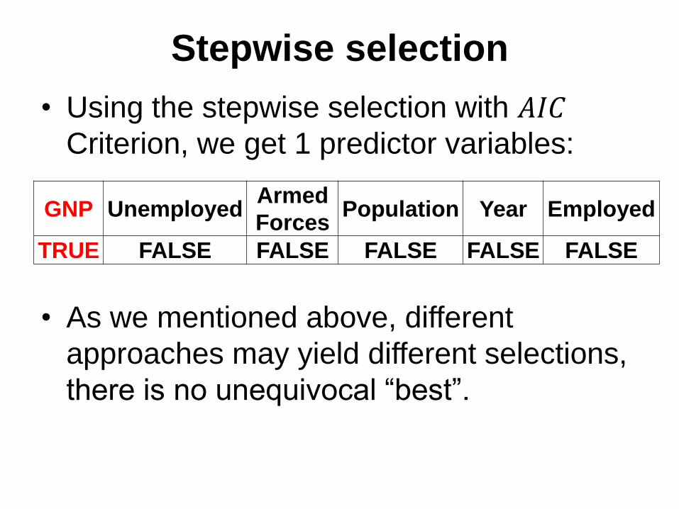
Stepwise selection
• Using the stepwise selection with 𝐴𝐼𝐶
Criterion, we get 1 predictor variables:
• As we mentioned above, different
approaches may yield different selections,
there is no unequivocal “best”.
GNP Unemployed Armed
Forces Population Year Employed
TRUE FALSE FALSE FALSE FALSE FALSE

Regression in Excel: LINEST(…)

Exercises with SAS
• Use SAS Proc Regression