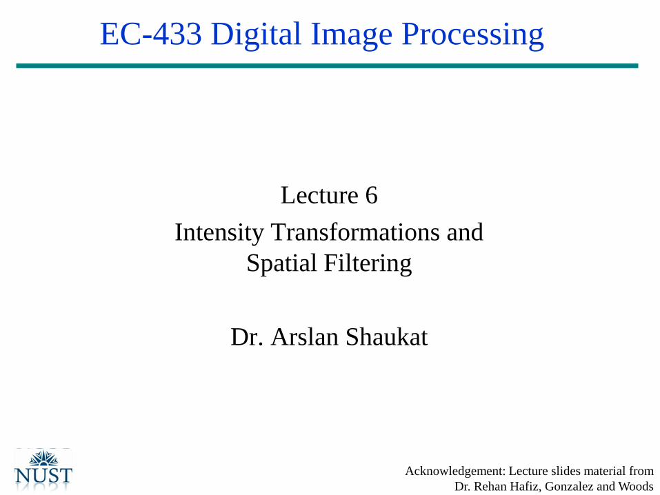
EC-433 Digital Image Processing

Lecture 6

Intensity Transformations and

Spatial Filtering

Dr. Arslan Shaukat

Acknowledgement: Lecture slides material from

Dr. Rehan Hafiz, Gonzalez and Woods

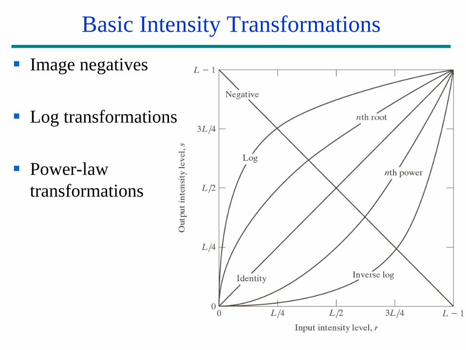
Basic Intensity Transformations

Image negatives

Log transformations

Power-law

transformations

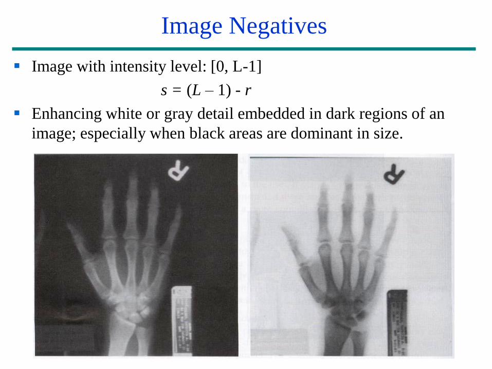
Image Negatives

Image with intensity level: [0, L-1]

s = (L – 1) - r

Enhancing white or gray detail embedded in dark regions of an

image; especially when black areas are dominant in size.

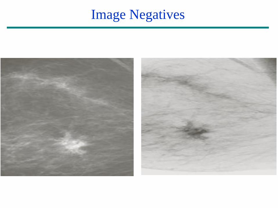
Image Negatives

Log Transformations

s = clog(1 + r)

– c = constant

– r greater than or equal to 0

Useful for low contrast

dark images

Log Transformations

Properties of log transformations

– For lower amplitudes of input image the range of gray levels is

expanded

– For higher amplitudes of input image the range of gray levels is

compressed

Application:

– This transformation is suitable for the case when the dynamic

range of a processed image far exceeds the capability of the

display device (e.g. display of the Fourier spectrum of an

image)

– Also called “dynamic-range compression/expansion”

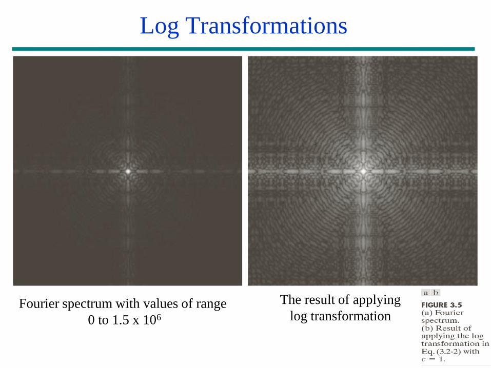
Fourier spectrum with values of range

0 to 1.5 x 106

Log Transformations

The result of applying

log transformation

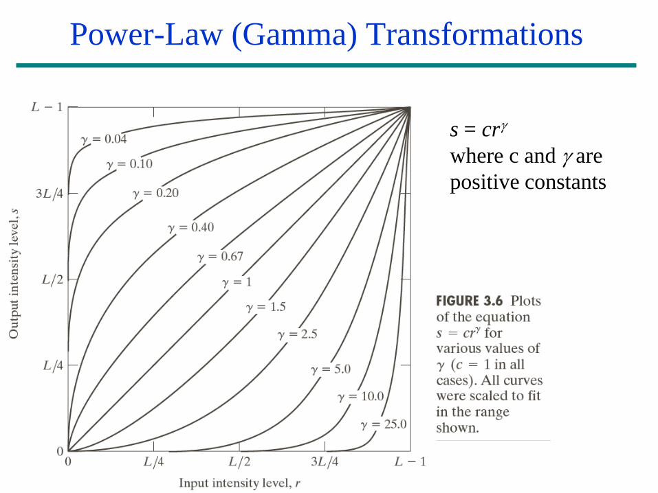
Power-Law (Gamma) Transformations

)],(.[),( yxIcyxg

s = cr

where c and are

positive constants

Used to adjust contrast of an image by either expanding

or compressing gray levels

– γ< 1, gray-level expansion

– γ> 1, gray-level compression

– If γ=1 & c=1, identity transformation (s = r)

More versatile as compared to logarithmic curve

Gamma Function

Power Law Transformations

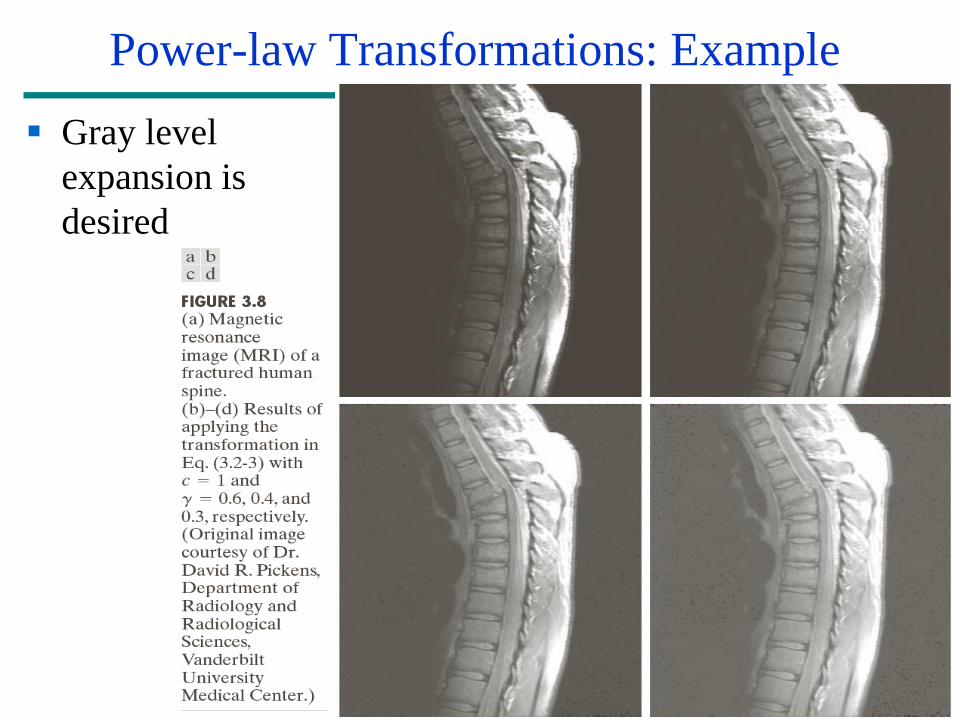
Power-law Transformations: Example

Gray level

expansion is

desired

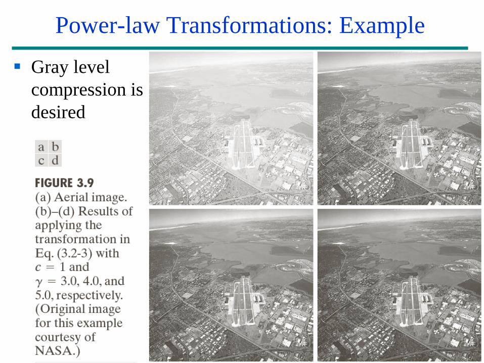
Power-law Transformations: Example

Gray level

compression is

desired

Gamma Correction

A variety of devices used for image capture, printing,

display respond according to a power law and need to be

corrected

Gamma (γ) correction

– The process used to correct the power-law response

phenomena

Example of gamma correction

– Cathode ray tube response is non linear (is a power function)

– To linearise the CRT response, pre-process the input image

before inputting it into the monitor by using transformation

s = cr1/γ

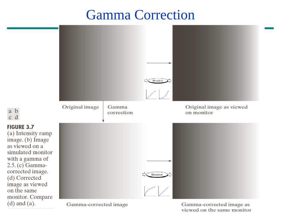
Gamma Correction

Piecewise-linear Transformation Functions

Contrast stretching

Intensity-level slicing

Bit-plane slicing

The principal advantage is that the form of piecewise

functions can be arbitrarily complex.

Contrast Stretching

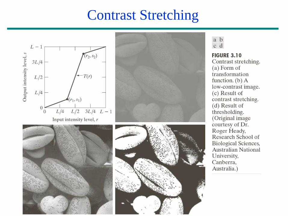
Goal:

Increase the dynamic range of the gray levels for low

contrast images so that it spans the full intensity range

Low-contrast images can result from

– poor illumination

– lack of dynamic range in the imaging sensor

– wrong setting of a lens aperture during image acquisition

Contrast Stretching

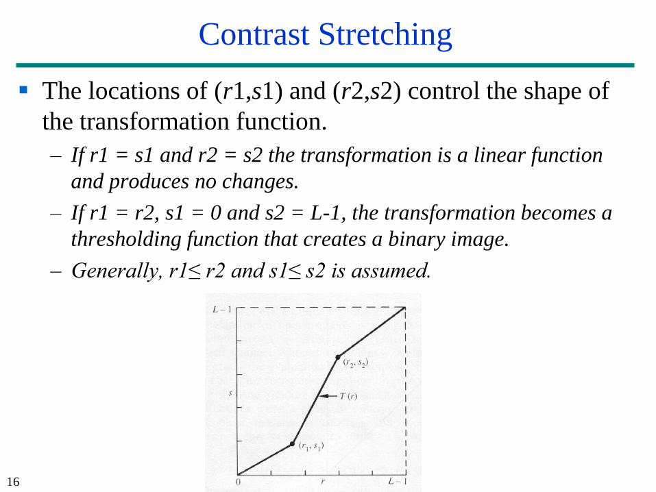
The locations of (r1,s1) and (r2,s2) control the shape of

the transformation function.

– If r1 = s1 and r2 = s2 the transformation is a linear function

and produces no changes.

– If r1 = r2, s1 = 0 and s2 = L-1, the transformation becomes a

thresholding function that creates a binary image.

– Generally, r1≤ r2 and s1≤ s2 is assumed.

16

Contrast Stretching

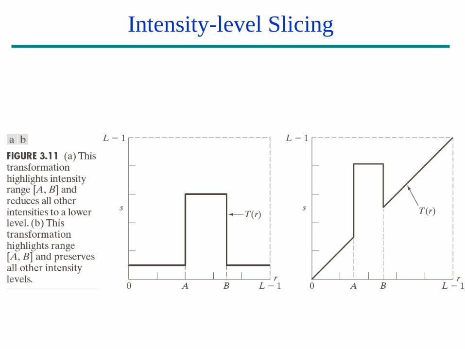
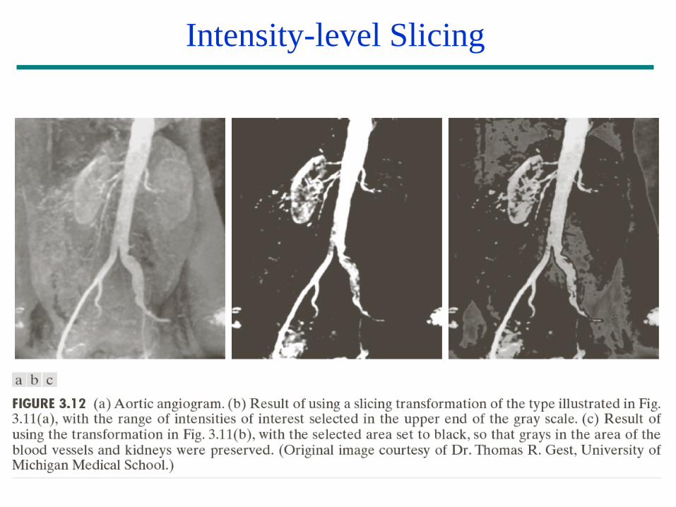
Intensity-level Slicing

To highlight a specific range of gray levels in an image

(e.g. to enhance certain features).

One way is to display a high value for all gray levels in

the range of interest and a low value for all other gray

levels (binary image).

The second approach is to brighten the desired range of

gray levels but preserve the background and gray-level

tonalities in the image.

Intensity-level Slicing

Intensity-level Slicing

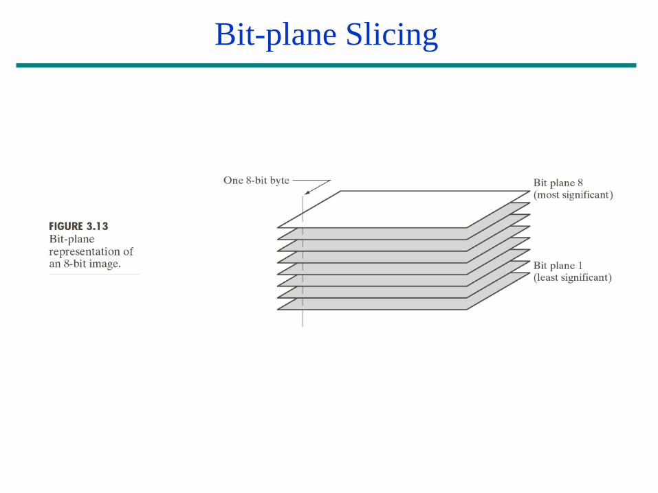
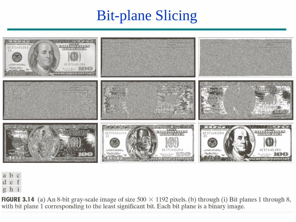
Bit-plane Slicing

To highlight the contribution made to the total image

appearance by specific bits.

– i.e. Assuming that each pixel is represented by 8 bits, the image

is composed of 8 1-bit planes.

– Plane 1 contains the least significant bit and plane 8 contains

the most significant bit.

– Useful for analyzing the relative importance played by each bit

of the image

– Only the higher order bits (top four) contain visually significant

data. The other bit planes contribute the more subtle details

– Plane 8 corresponds exactly with an image thresholded at gray

level 128

Bit-plane Slicing

Bit-plane Slicing

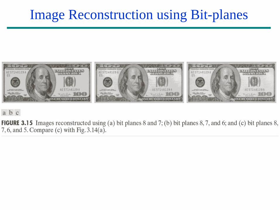
Image Reconstruction using Bit-planes