lecture 6 – quantitative process analysis ii

MTAT.03.231 Business Process Management

Lecture 6 – Quantitative Process

Analysis II

Marlon Dumas

marlon.dumas ät ut . ee

1

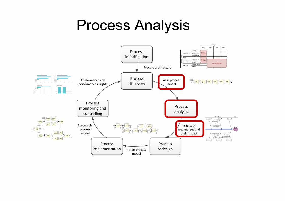
Process Analysis Process

identification

Conformance and performance insightsConformance and

performance insights

Processmonitoring and controlling

Executable processmodel


Processimplementation To-‐be process

modelTo-‐be process

model

Processanalysis

As-‐is processmodel


Process discovery

Process architectureProcess architecture

Processredesign

Insights onweaknesses and their impact


Process Analysis Techniques

Qualitative analysis •  Value-Added & Waste Analysis •  Root-Cause Analysis •  Pareto Analysis •  Issue Register

Quantitative Analysis •  Flow analysis •  Queuing analysis •  Simulation

1.  Introduction 2.  Process Identification 3.  Essential Process Modeling 4.  Advanced Process Modeling 5.  Process Discovery 6.  Qualitative Process Analysis 7.  Quantitative Process Analysis 8.  Process Redesign 9.  Process Automation 10. Process Intelligence

Flow analysis does not consider

wai0ng 0mes due to resource conten0on

Queuing analysis and simula0on address these limita0ons and have a broader applicability

Why flow analysis is not enough?

• Capacity problems are common and a key driver of process redesign •  Need to balance the cost of increased capacity against the gains of

increased productivity and service • Queuing and waiting time analysis is particularly

important in service systems •  Large costs of waiting and/or lost sales due to waiting

Prototype Example – ER at a Hospital • Patients arrive by ambulance or by their own accord • One doctor is always on duty • More patients seeks help ⇒ longer waiting times Ø Question: Should another MD position be instated?

Queuing Analysis

© Laguna & Marklund

If arrivals are regular or sufficiently spaced apart, no queuing delay occurs

Delay is Caused by Job Interference

Deterministic traffic

Variable but spaced apart traffic

Time

Arrival Times

Departure Times

1 3 42

1 3 42

Time

Arrival Times

Departure Times

1 3 42

1 3 42

© Dimitri P. Bertsekas

Burstiness Causes Interference

Time

Queuing Delays

Bursty Traffic

1 2 3 4

1 2 3 4

*  Queuing results from variability in processing times and/or interarrival intervals


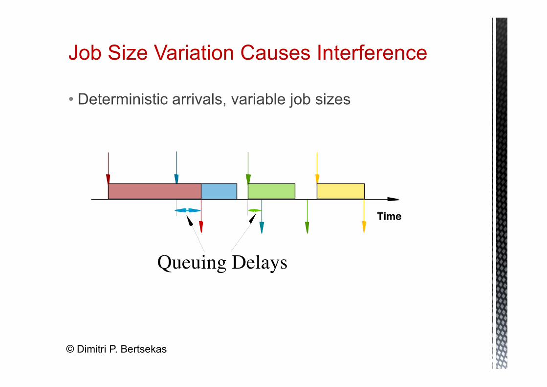
• Deterministic arrivals, variable job sizes

Job Size Variation Causes Interference

Time

Queuing Delays


• The queuing probability increases as the load increases • Utilization close to 100% is unsustainable à too long

queuing times

High Utilization Exacerbates Interference

Time

Queuing Delays


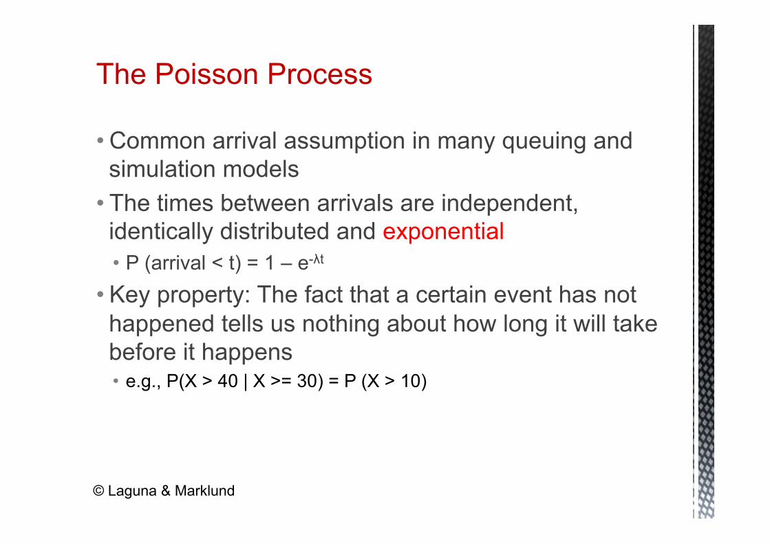
• Common arrival assumption in many queuing and simulation models

• The times between arrivals are independent, identically distributed and exponential • P (arrival < t) = 1 – e-λt

• Key property: The fact that a certain event has not happened tells us nothing about how long it will take before it happens •  e.g., P(X > 40 | X >= 30) = P (X > 10)

The Poisson Process


Negative Exponential Distribution

Basic characteristics: • λ (mean arrival rate) = average number of arrivals per

time unit • µ (mean service rate) = average number of jobs that can

be handled by one server per time unit: • c = number of servers

Queuing theory: basic concepts

arrivals waiting service

λ µ c

© Wil van der Aalst

Given λ , µ and c, we can calculate : •  occupation rate: ρ •  Wq = average time in queue •  W = average system in system (i.e. cycle time) •  Lq = average number in queue (i.e. length of queue) •  L = average number in system average (i.e. Work-in-Progress)

Queuing theory concepts (cont.)

λ µ c

Wq,Lq

W,L

© Wil van der Aalst

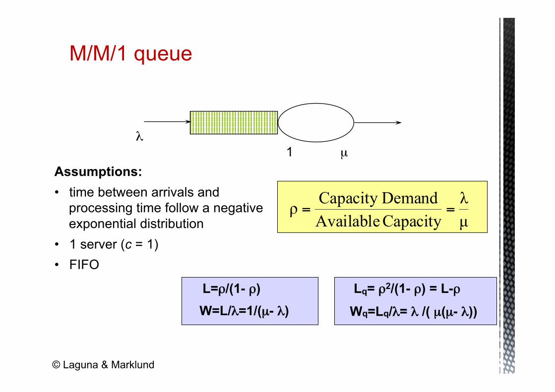
M/M/1 queue

λ µ 1

Assumptions: •  time between arrivals and

processing time follow a negative exponential distribution

•  1 server (c = 1) •  FIFO

L=ρ/(1- ρ) Lq= ρ2/(1- ρ) = L-ρ W=L/λ=1/(µ- λ) Wq=Lq/λ= λ /( µ(µ- λ))

µλ

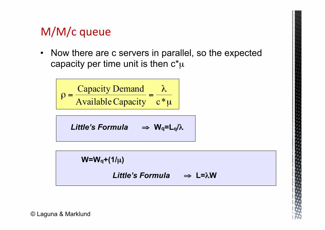
CapacityAvailableDemandCapacityρ ==


µλ

==ρ*cCapacityAvailable

DemandCapacity

•  Now there are c servers in parallel, so the expected capacity per time unit is then c*µ

W=Wq+(1/µ)

Little’s Formula ⇒ Wq=Lq/λ

Little’s Formula ⇒ L=λW


M/M/c queue

• For M/M/c systems, the exact computation of Lq is rather complex…

• Consider using a tool, e.g.

• http://queueingtoolpak.org/ (for Excel) http://www.stat.auckland.ac.nz/~stats255/qsim/qsim.html

Tool Support

02

c

cnnq P

)1(!c)/(...P)cn(Lρ−

ρµλ==−= ∑

∞

=

1c1c

0n

n

0 )c/((11

!c)/(

!n)/(P

−−

=⎟⎟⎠

⎞⎜⎜⎝

⎛

µλ−⋅

µλ+

µλ= ∑

Ø  Situation •  Patients arrive according to a Poisson process with intensity λ

(⇔ the time between arrivals is exp(λ) distributed. •  The service time (the doctor’s examination and treatment time

of a patient) follows an exponential distribution with mean 1/µ (=exp(µ) distributed)

⇒  The ER can be modeled as an M/M/c system where c = the number of doctors

Ø  Data gathering ⇒  λ = 2 pa0ents per hour ⇒  µ = 3 pa0ents per hour

v  Ques0on –  Should the capacity be increased from 1 to 2 doctors?

Example – ER at County Hospital


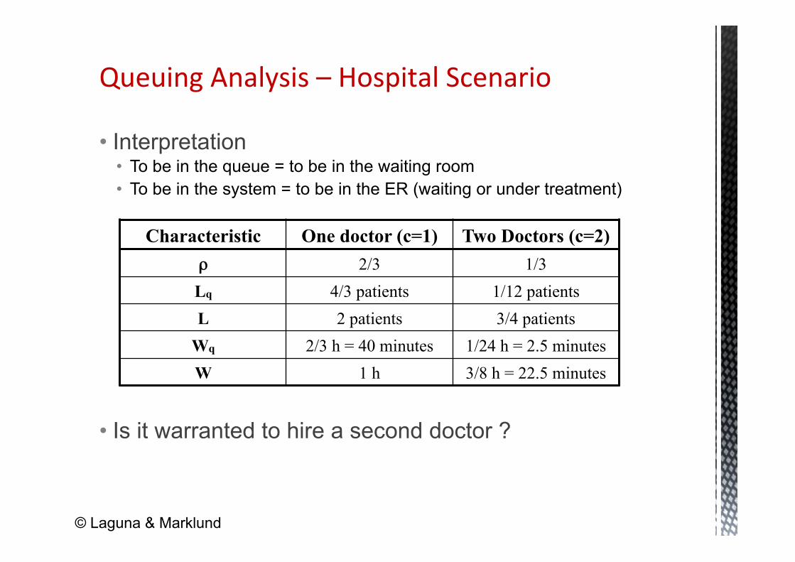
•  Interpretation •  To be in the queue = to be in the waiting room •  To be in the system = to be in the ER (waiting or under treatment)

•  Is it warranted to hire a second doctor ?

Queuing Analysis – Hospital Scenario

Characteristic One doctor (c=1) Two Doctors (c=2) ρ 2/3 1/3 Lq 4/3 patients 1/12 patients L 2 patients 3/4 patients

Wq 2/3 h = 40 minutes 1/24 h = 2.5 minutes W 1 h 3/8 h = 22.5 minutes


• Textbook, Chapter 7, exercise 7.12 (page 249)

Your turn

Simula0on

21

•  Versatile quantitative analysis method for •  As-is analysis •  What-if analysis

•  In a nutshell: •  Run a large number of process instances •  Gather performance data (cost, time, resource usage) •  Calculate statistics from the collected data

Process Simulation

Process Simulation

Model the process

Define a simula0on scenario

Run the simula0on

Analyze the simula0on outputs

Repeat for alterna0ve scenarios

Example

Elements of a simulation scenario

1.  Processing times of activities •  Fixed value •  Probability distribution

Exponential Distribution

Normal Distribution

• Fixed • Rare, can be used to approximate case where the ac0vity processing 0me varies very liWle

• Example: a task performed by a soYware applica0on • Normal

• Repe00ve ac0vi0es • Example: “Check completeness of an applica0on”

• Exponen0al • Complex ac0vi0es that may involve analysis or decisions • Example: “Assess an applica0on”

Choice of probability distribu0on

29

Simulation Example

Exp(20m)

Normal(20m, 4m)

Normal(10m, 2m) Normal(10m, 2m)

Normal(10m, 2m)

0m

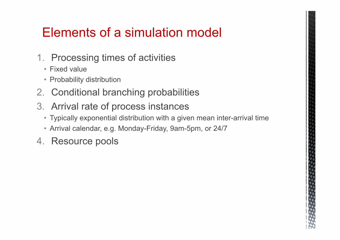
Elements of a simulation model


2.  Conditional branching probabilities 3.  Arrival rate of process instances and probability distribution

•  Typically exponential distribution with a given mean inter-arrival time •  Arrival calendar, e.g. Monday-Friday, 9am-5pm, or 24/7

Branching probability and arrival rate Arrival rate = 2 applications per hour

Inter-arrival time = 0.5 hour Negative exponential distribution From Monday-Friday, 9am-5pm

0.3

0.7

0.3

9:00 10:00 11:00 12:00 13:00 13:00

35m 55m



2.  Conditional branching probabilities 3.  Arrival rate of process instances


4.  Resource pools

Resource pools

• Name • Size of the resource pool • Cost per time unit of a resource in the pool • Availability of the pool (working calendar) • Examples

•  Clerk Credit Officer •  € 25 per hour € 25 per hour •  Monday-Friday, 9am-5pm Monday-Friday, 9am-5pm

•  In some tools, it is possible to define cost and calendar per resource, rather than for entire resource pool



2.  Conditional branching probabilities 3.  Arrival rate of process instances and probability distribution


4.  Resource pools 5.  Assignment of tasks to resource pools

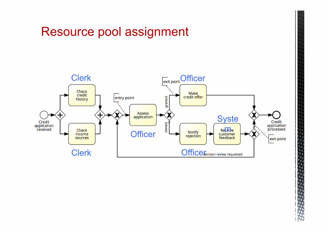
Resource pool assignment

Officer

Clerk

Clerk Officer

Officer

System

Process Simulation

Model the process


Run the simula0on



✔ ✔ ✔

Output: Performance measures & histograms

Process Simulation

Model the process


Run the simula0on



✔ ✔ ✔

✔

Tools for Process Simula0on

• ARIS • Bizagi Process Modeler •  ITP Commerce Process Modeler for Visio • Logizian • Oracle BPA • Progress Savvion Process Modeler • ProSim • Signavio + BIMP

BIMP – bimp.cs.ut.ee

• Accepts standard BPMN 2.0 as input • Simple form-‐based interface to enter simula0on scenario • Produces KPIs + simula0on logs in MXML format

•  Simula0on logs can be imported to the ProM process mining tool

BIMP Demo

• Textbook, Chapter 7, exercise 7.8 (page 240)

Your turn

• Stochas0city • Data quality piialls • Simplifying assump0ons

Piialls of simula0on

44

• Simula0on results may differ from one run to another • Make the simula0on 0emframe long enough to cover weekly and seasonal variability, where applicable

• Use mul0ple simula0on runs • Average results of mul0ple runs, compute confidence intervals

Stochas0city

45

• Simula0on results are only as trustworthy as the input data • Rely as liWle as possible on “guess0mates” • Use input analysis

•  Deriver simula0on scenario parameters from numbers in the scenario •  Use sta0s0cal tools to check fit the probability distribu0ons

• Simulate the “as is” scenario and cross-‐check results against actual observa0ons

Data quality piialls

46

• That the process model is always followed to the leWer •  No devia0ons •  No workarounds

• That resources work constantly and non-‐stop •  Every day is the same! •  No 0redness effects •  No distrac0ons beyond “stochas0c” ones

Simula0on assump0ons

47

Next week

Process identification

Conformance and performance insightsConformance and

performance insights

Processmonitoring and controlling



Processimplementation To-‐be process

modelTo-‐be process

model

Processanalysis



Process discovery

Process architectureProcess architecture

Processredesign



lecture 6 – quantitative process analysis ii

Documents