Lecture 7: ANOVA

Sandy Eckelseckel@jhsph.edu

30 April 2008

1 / 34

Statistical methods for comparing multiple groups

Continuous data: comparing multiple means

Analysis of variance

Binary data: comparing multiple proportions

Chi-square tests for r × 2 tables

IndependenceGoodness of FitHomogeneity

Categorical data: comparing multiple sets of categorical responses

Similar chi-square tests for r × c tables

2 / 34

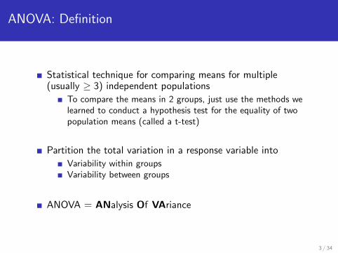
ANOVA: Definition

Statistical technique for comparing means for multiple(usually ≥ 3) independent populations

To compare the means in 2 groups, just use the methods welearned to conduct a hypothesis test for the equality of twopopulation means (called a t-test)

Partition the total variation in a response variable into

Variability within groupsVariability between groups

ANOVA = ANalysis Of VAriance

3 / 34

ANOVA: Concepts

Estimate group means

Assess magnitude of variation attributable to specific sources

Partition the variation according to source

Extension of 2-sample t-test to multiple groups

Population model

Sample model: sample estimates,standard errors (sd of sampling distribution)

4 / 34

Types of ANOVA

One-way ANOVA

One factor — e.g. smoking status(never, former, current)

Two-way ANOVA

Two factors — e.g. gender and smoking status

Three-way ANOVA

Three factors — e.g. gender, smoking and beer consumption

5 / 34

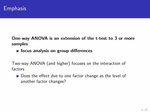
Emphasis

One-way ANOVA is an extension of the t-test to 3 or moresamples

focus analysis on group differences

Two-way ANOVA (and higher) focuses on the interaction offactors

Does the effect due to one factor change as the level ofanother factor changes?

6 / 34

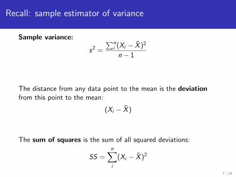
Recall: sample estimator of variance

Sample variance:

s2 =

∑ni (Xi − X̄ )2

n − 1

The distance from any data point to the mean is the deviationfrom this point to the mean:

(Xi − X̄ )

The sum of squares is the sum of all squared deviations:

SS =n∑i

(Xi − X̄ )2

7 / 34

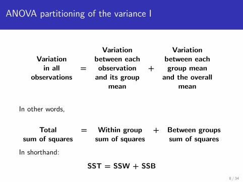
ANOVA partitioning of the variance I

Variation VariationVariation between each between each

in all = observation + group meanobservations and its group and the overall

mean mean

In other words,

Total = Within group + Between groupssum of squares sum of squares sum of squares

In shorthand:

SST = SSW + SSB

8 / 34

ANOVA partitioning of the variance II

SST This is the sum of the squared deviations betweeneach observation and the overall mean:

SST =n∑i

(Xi − X̄ )2

SSW This is the sum of the squared deviations betweeneach observation the mean of the group to which itbelongs:

SSW =n∑i

(Xi − X̄group(i))2

9 / 34

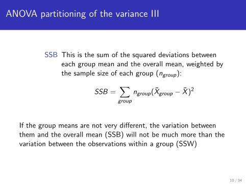
ANOVA partitioning of the variance III

SSB This is the sum of the squared deviations betweeneach group mean and the overall mean, weighted bythe sample size of each group (ngroup):

SSB =∑group

ngroup(X̄group − X̄ )2

If the group means are not very different, the variation betweenthem and the overall mean (SSB) will not be much more than thevariation between the observations within a group (SSW)

10 / 34

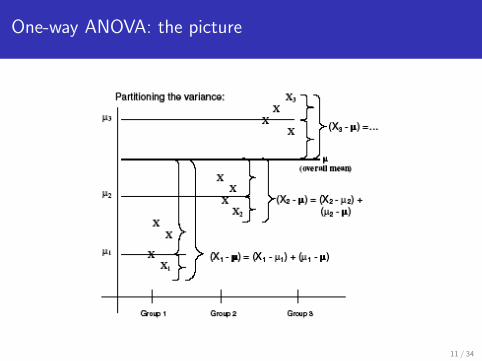
One-way ANOVA: the picture

11 / 34

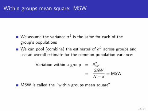
Within groups mean square: MSW

We assume the variance σ2 is the same for each of thegroup’s populations

We can pool (combine) the estimates of σ2 across groups anduse an overall estimate for the common population variance:

Variation within a group = σ̂2W

=SSW

N − k= MSW

MSW is called the “within groups mean square”

12 / 34

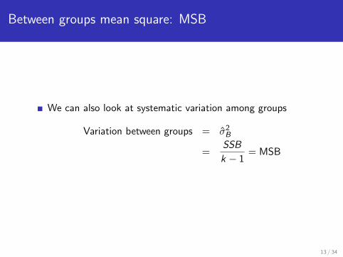
Between groups mean square: MSB

We can also look at systematic variation among groups

Variation between groups = σ̂2B

=SSB

k − 1= MSB

13 / 34

An ANOVA table

Suppose there are k groups (e.g. if smoking status hascategories current, former or never, then k=3)

We calculate a test statistic for a hypothesis test using thesum of square values as follows:

14 / 34

Hypothesis testing with ANOVA

In ANOVA we ask:is there truly a difference in means across groups?

Formally, we can specify the hypotheses:

H0 : µ1 = µ2 = · · · = µk

Ha : at least one of the µi ’s is different

The null hypothesis specifies a global relationship between themeans

Get your test statistic (more next slide...)

If the result of the test is significant (p-value ≤ α),then perform individual comparisons between pairs of groups

15 / 34

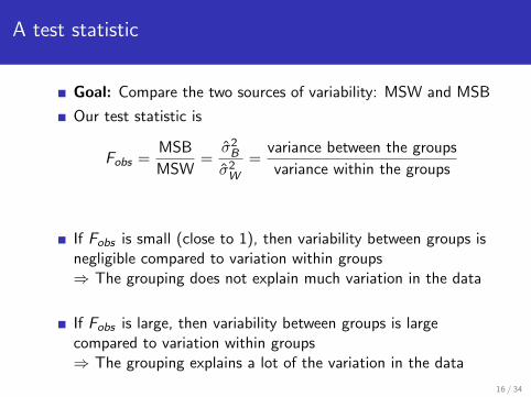
A test statistic

Goal: Compare the two sources of variability: MSW and MSB

Our test statistic is

Fobs =MSB

MSW=σ̂2

B

σ̂2W

=variance between the groups

variance within the groups

If Fobs is small (close to 1), then variability between groups isnegligible compared to variation within groups⇒ The grouping does not explain much variation in the data

If Fobs is large, then variability between groups is largecompared to variation within groups⇒ The grouping explains a lot of the variation in the data

16 / 34

The F-statistic

For our observations, we assume X ∼ N(µgp, σ2), where µgp

is the (possibly different) mean for each group’s population.

Note: under H0, we assume all the group means are the same

We have assumed the same variance σ2 for all groups —important to check this assumption

Under these assumptions, we know the null distribution of thestatistic F= MSB

MSW

The distribution is called an F-distribution

17 / 34

The F-distribution

Remember that a χ2 distribution is always specified by itsdegrees of freedom

An F-distribution is any distribution obtained by taking thequotient of two χ2 distributions divided by their respectivedegrees of freedom

When we specify an F-distribution, we must state twoparameters, which correspond to the degrees of freedom forthe two χ2 distributions

If X1 ∼ χ2df1

and X2 ∼ χ2df2

we write:

X1/df1X2/df2

∼ Fdf1,df2

18 / 34

Back to the hypothesis test . . .

Knowing the null distribution of MSBMSW, we can define a decision

rule for the ANOVA test statistic (Fobs):

Reject H0 if Fobs ≥ Fα;k−1,N−k

Fail to reject H0 if Fobs < Fα;k−1,N−k

Fα;k−1,N−k is the value on the Fk−1,N−k distribution that,used as a cutoff, gives an area in the uppper tail = α

We are using a one-sided rejection region

19 / 34

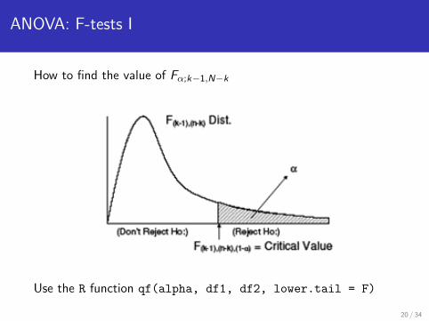
ANOVA: F-tests I

How to find the value of Fα;k−1,N−k

Use the R function qf(alpha, df1, df2, lower.tail = F)

20 / 34

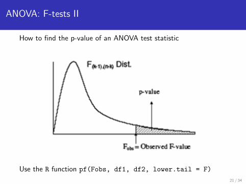
ANOVA: F-tests II

How to find the p-value of an ANOVA test statistic

Use the R function pf(Fobs, df1, df2, lower.tail = F)

21 / 34

Example: ANOVA for HDL

Study design: Randomized controlled trial

132 men randomized to one of

Diet + exericseDietControl

Follow-up one year later:

119 men remaining in study

Outcome: mean change in plasma levels of HDL cholesterol frombaseline to one-year follow-up in the three groups

22 / 34

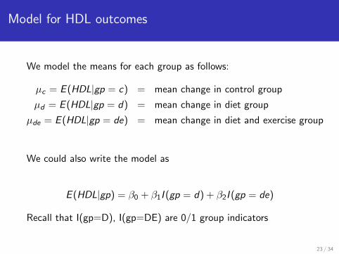
Model for HDL outcomes

We model the means for each group as follows:

µc = E (HDL|gp = c) = mean change in control group

µd = E (HDL|gp = d) = mean change in diet group

µde = E (HDL|gp = de) = mean change in diet and exercise group

We could also write the model as

E (HDL|gp) = β0 + β1I (gp = d) + β2I (gp = de)

Recall that I(gp=D), I(gp=DE) are 0/1 group indicators

23 / 34

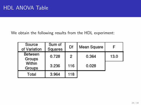
HDL ANOVA Table

We obtain the following results from the HDL experiment:

24 / 34

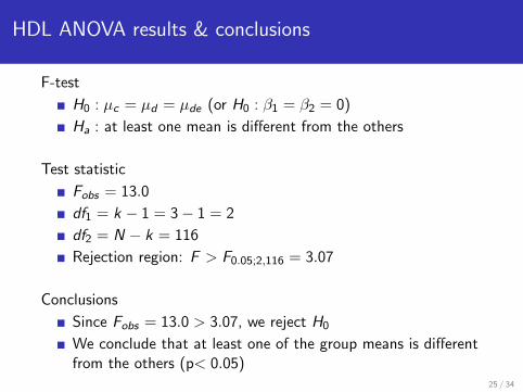
HDL ANOVA results & conclusions

F-test

H0 : µc = µd = µde (or H0 : β1 = β2 = 0)

Ha : at least one mean is different from the others

Test statistic

Fobs = 13.0

df1 = k − 1 = 3− 1 = 2

df2 = N − k = 116

Rejection region: F > F0.05;2,116 = 3.07

Conclusions

Since Fobs = 13.0 > 3.07, we reject H0

We conclude that at least one of the group means is differentfrom the others (p< 0.05)

25 / 34

Which groups are different?

We might proceed to make individual comparisons

Conduct two-sample t-tests to test for a difference in meansfor each pair of groups (assuming equal variance):

tobs =(X̄1 − X̄2)− µ0√

s2p

n1+

s2p

n2

Recall: s2p is the ‘pooled’ sample estimate of the common

variance

df = n1 + n2 − 2

26 / 34

Multiple Comparisons

Performing individual comparisons require multiple hypothesistests

If α = 0.05 for each comparison, there is a 5% chance thateach comparison will falsely be called significant

Overall, the probability of Type I error is elevated above 5%

For n independent tests, the probability of making a Type Ierror at least once is 1− 0.95n

Example: For n = 10 tests, the probability of at least oneType I error is 0.40 !

Question: How can we address this multiple comparisonsissue?

27 / 34

Bonferroni adjustment

A possible correction for multiple comparisons

Test each hypothesis at level α∗ = (α/3) = 0.0167

Adjustment ensures overall Type I error rate does not exceedα = 0.05

However, this adjustment may be too conservative

28 / 34

Multiple comparisons α

Hypothesis α∗ = α/3

H0 : µc = µd (or β1 = 0) 0.0167H0 : µc = µde (or β2 = 0) 0.0167H0 : µd = µde (or β1 − β2 = 0) 0.0167

Overall α = 0.05

29 / 34

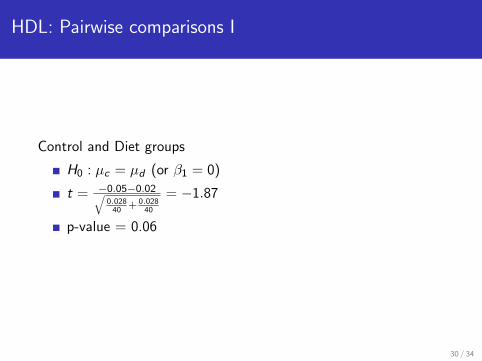
HDL: Pairwise comparisons I

Control and Diet groups

H0 : µc = µd (or β1 = 0)

t = −0.05−0.02√0.028

40+ 0.028

40

= −1.87

p-value = 0.06

30 / 34

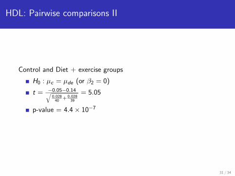
HDL: Pairwise comparisons II

Control and Diet + exercise groups

H0 : µc = µde (or β2 = 0)

t = −0.05−0.14√0.028

40+ 0.028

39

= 5.05

p-value = 4.4× 10−7

31 / 34

HDL: Pairwise comparisons III

Diet and Diet + exercise groups

H0 : µd = µde (or β1 − β2 = 0)

t = −0.02−0.14√0.028

40+ 0.028

39

= −3.19

p-value = 0.0014

32 / 34

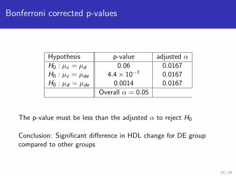
Bonferroni corrected p-values

Hypothesis p-value adjusted α

H0 : µc = µd 0.06 0.0167H0 : µc = µde 4.4× 10−7 0.0167H0 : µd = µde 0.0014 0.0167

Overall α = 0.05

The p-value must be less than the adjusted α to reject H0

Conclusion: Significant difference in HDL change for DE groupcompared to other groups

33 / 34

Summary of Lecture 7

Sample variance, sums of squares

ANOVA

partition of the sums of squaresANOVA tablehypothesis test setuptest statistic

F distribution

Multiple hypothesis testing, Bonferroni correction

ANOVA ”dull hypothesis” joke:http://www.phdcomics.com/comics/archive.php?comicid=905

34 / 34