Lecture 7a: Vector Autoregression (VAR)

1

Big Picture

• We are done with univariate time series analysis

• Now we switch to multivariate analysis, that is, studying several

time series simultaneously.

• VAR is one of the most popular multivariate models

2

VAR(1)

• Consider a bivariate system (yt, xt).

• For example, yt is the inflation rate, and xt is the unemployment

rate. The relationship between them is Phillips Curve.

• The first order VAR for this bivariate system is

yt = ϕ11yt−1 + ϕ12xt−1 + ut (1)

xt = ϕ21yt−1 + ϕ22xt−1 + vt (2)

So each variable depends on the first lag of itself and the other

variable.

3

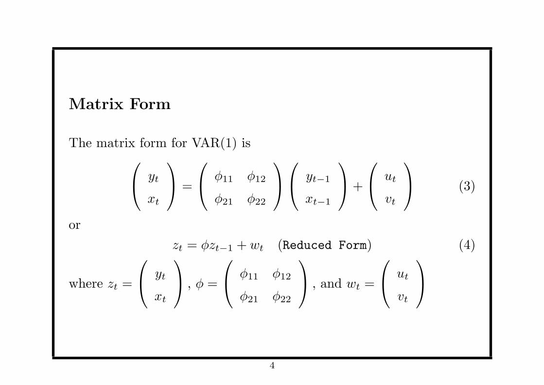
Matrix Form

The matrix form for VAR(1) is yt

xt

=

ϕ11 ϕ12

ϕ21 ϕ22

yt−1

xt−1

+

ut

vt

(3)

or

zt = ϕzt−1 + wt (Reduced Form) (4)

where zt =

yt

xt

, ϕ =

ϕ11 ϕ12

ϕ21 ϕ22

, and wt =

ut

vt

4

Stationarity Condition

1. (yt, xt) are both stationary when the eigenvalues of ϕ are less

than one in absolute value.

2. (yt, xt) are both integrated of order one, and yt and xt are

cointegrated when one eigenvalue is unity, and the other

eigenvalue is less than one in absolute value.

3. (yt, xt) are both integrated of order two if both eigenvalues of ϕ

are unity.

5

OLS Estimation

1. Each equation in the VAR can be estimated by OLS.

2. Then the variance covariance matrix for the error vector

Ω = Ewtw′t =

σ2u σu,v

σu,v σ2v

can be estimated by

Ω = T−1

∑u2t

∑utvt∑

utvt∑

v2t

where ut and vt are residuals.

6

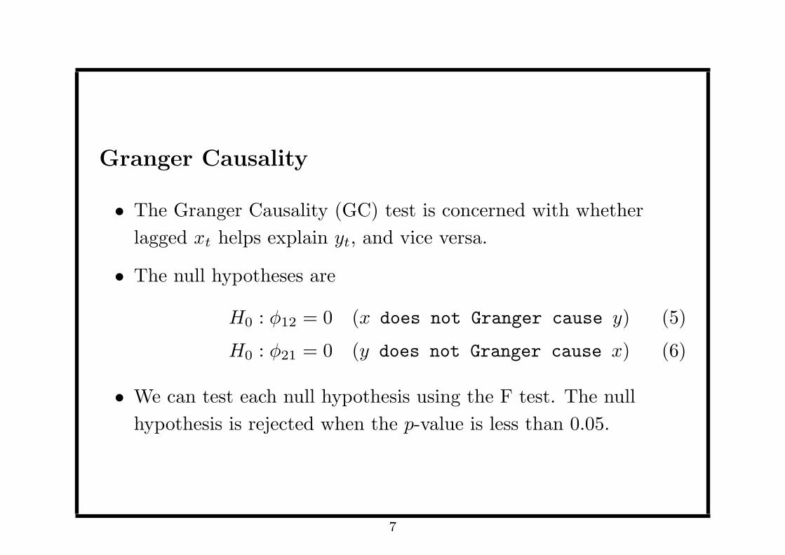
Granger Causality

• The Granger Causality (GC) test is concerned with whether

lagged xt helps explain yt, and vice versa.

• The null hypotheses are

H0 : ϕ12 = 0 (x does not Granger cause y) (5)

H0 : ϕ21 = 0 (y does not Granger cause x) (6)

• We can test each null hypothesis using the F test. The null

hypothesis is rejected when the p-value is less than 0.05.

7

Warning

• Granger Causality = Causality.

• Granger causality is about in-sample fitting. It tells nothing

about out-of-sample forecasting.

8

Impulse Response

• Using the lag operator we can show the MA(∞) representation

for the VAR(1) is

zt = wt + ϕwt−1 + ϕ2wt−2 + . . .+ ϕjwt−j + . . . (7)

• The coefficient in the MA representation measures the impulse

response:

ϕj =dzt

dwt−j(8)

Note ϕj is a 2× 2 matrix for a bivariate system.

9

Impulse Response II

• More generally, denote the (m,n)-th component of ϕj by

ϕj(m,n)

• Then ϕj(m,n) measures the response of m-th variable to the

n-th error after j periods.

• For example, ϕ3(1, 2) measures the response of first variable to

the error of the second variable after 3 periods.

10

Impulse Response III

• We can plot the impulse response against j. That is, for a given

impulse response plot, we let j varies while holding m and n

constant.

• For a bivariate system, there are four impulse responses plots.

11

Impulse Response IV

• In general ut and vt are contemporaneously correlated

(not-orthogonal), i.e., σu,v = 0

• Therefore we can not, say, hold v constant and let only u vary.

• However, we can always find a lower triangular matrix A so that

Ω = AA′ (Cholesky Decomposition) (9)

• Then define a new error vector wt as (linear transformation of

old error vector wt)

wt = A−1wt (10)

• By construction the new error is orthogonal because its

variance-covariance matrix is diagonal:

var(wt) = A−1var(wt)A−1′ = A−1ΩA−1′ = A−1AA′A−1′ = I

12

Cholesky Decomposition

Let A =

a 0

b c

. The Cholesky Decomposition tries to solve

a 0

b c

a b

0 c

=

σ2u σu,v

σu,v σ2v

The solutions for a, b, c always exist and they are

a =√σ2u (11)

b =σu,v√σ2u

(12)

c =

√σ2v −

σ2u,v

σ2u

(13)

13

Positive Definite Matrix

Note c is always a real number since Ω is a variance-covariance

matrix, and so is positive definite (i.e., σ2v −

σ2u,v

σ2u

is always positive

because the determinant of Ω, or the second leading principal minor,

is positive).

14

Impulse Response to Orthogonal Errors

Rewrite the MA(∞) representation as

zt = wt + ϕwt−1 + . . .+ ϕjwt−j + . . . (14)

= AA−1wt + ϕAA−1wt−1 + . . .+ ϕjAA−1wt−j + . . . (15)

= Awt + ϕAwt−1 + . . .+ ϕjAwt−j + . . . (16)

This implies that the impulse response to the orthogonal error wt

after j periods is

j-th orthogonal impulse response = ϕjA (17)

where A satisfies (9).

15

Reduced Form and Structural Form

1. (4) is called reduced form and the reduced form error wt is not

orthogonal.

2. The so called structural form is a linear transformation of the

reduced form:

zt = ϕzt−1 + wt (18)

⇒ A−1zt = A−1ϕzt−1 +A−1wt (19)

⇒ A−1zt = A−1ϕzt−1 + wt (20)

where the structural form error wt is orthogonal.

16

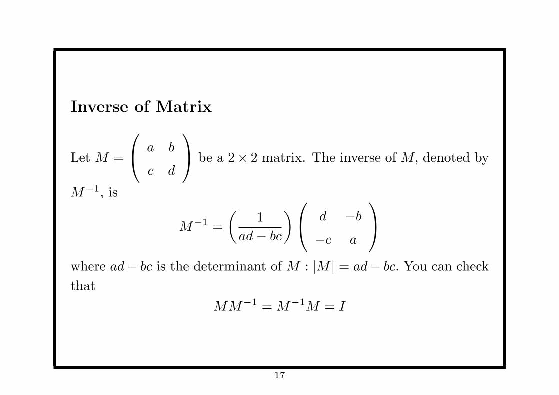
Inverse of Matrix

Let M =

a b

c d

be a 2× 2 matrix. The inverse of M, denoted by

M−1, is

M−1 =

(1

ad− bc

) d −b

−c a

where ad− bc is the determinant of M : |M | = ad− bc. You can check

that

MM−1 = M−1M = I

17

Structural Form

1. The Structural Form VAR is

A−1zt = A−1ϕzt−1 + wt (Structural Form) (21)

2. Note A−1 is lower triangular. So

A−1zt =

1/a 0

−b/(ac) 1/c

yt

xt

=

(1/a)yt

(−b/(ac))yt + (1/c)xt

3. That means xt will not appear in the regression for yt, whereas

yt will appear in the regression for xt.

4. This may not hold in practice.

18

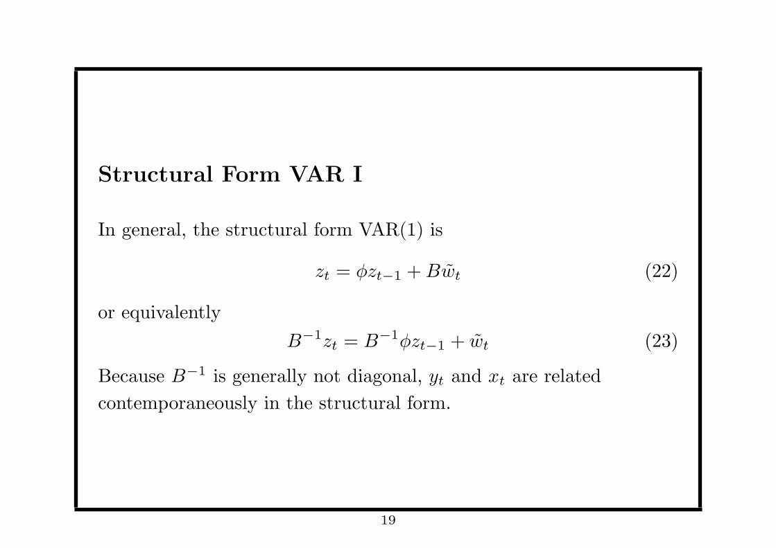
Structural Form VAR I

In general, the structural form VAR(1) is

zt = ϕzt−1 +Bwt (22)

or equivalently

B−1zt = B−1ϕzt−1 + wt (23)

Because B−1 is generally not diagonal, yt and xt are related

contemporaneously in the structural form.

19

Why is it called structural form?

1. Because in the structural VAR there is instantaneous interaction

between yt and xt.

2. Both yt and xt are endogenous, and the regressors include the

current value of endogenous variables in the structural form.

3. The structural VAR is one example of the simultaneous equation

model (SEM)

4. We cannot estimate the structural VAR using per-equation OLS,

due to the bias of simultaneity.

5. We can estimate the reduced form using per-equation OLS. Then

we recover the structural form from the reduced form, with

(identification) restriction imposed.

20

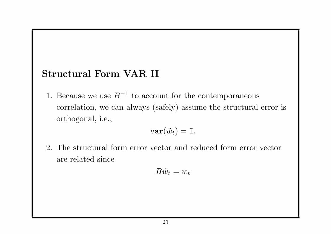
Structural Form VAR II

1. Because we use B−1 to account for the contemporaneous

correlation, we can always (safely) assume the structural error is

orthogonal, i.e.,

var(wt) = I.

2. The structural form error vector and reduced form error vector

are related since

Bwt = wt

21

Structural Form VAR III

1. Let Ω = E(wtw′t) be the observed variance covariance matrix. It

follows that

BB′ = Ω

2. The goal of structural VAR analysis is to obtain B, which is not

unique (for a bivariate system Ω has 3 unique elements, while B

has 4 elements to be determined).

3. The Sims (1980) structural VAR imposes the restriction that B

is lower triangular.

4. The Blanchard Quah structural VAR obtains B by looking at the

long run effect of the wt.

22

MA Representation

Consider a univariate AR(p)

yt = ϕ1yt−1 + . . .+ ϕpyt−p + et

Using the lag operator we can write

(1− ϕ1L− . . .+ ϕpLp)yt = et

We can obtain the MA representation by inverting the lag

polynomial (1− ϕ1L− . . .+ ϕpLp) :

yt = (1− ϕ1L− . . .+ ϕpLp)−1et

= et + θ1et−1 + θ2et−2 + . . .

23

Long Run Effect

The long run effect (LRE) of et is

LRE ≡ dytdet

+dyt+1

det+

dyt+2

det+ . . . (24)

= 1 + θ1 + θ2 + . . . (25)

= (1− ϕ1 − . . .+ ϕp)−1 (26)

In words, we need to invert the lag polynomial (1− ϕ1L− . . .+ ϕpLp)

after replacing L with number 1.

24

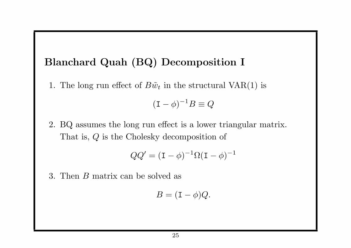
Blanchard Quah (BQ) Decomposition I

1. The long run effect of Bwt in the structural VAR(1) is

(I− ϕ)−1B ≡ Q

2. BQ assumes the long run effect is a lower triangular matrix.

That is, Q is the Cholesky decomposition of

QQ′ = (I− ϕ)−1Ω(I− ϕ)−1

3. Then B matrix can be solved as

B = (I− ϕ)Q.

25

Blanchard Quah (BQ) Decomposition II

In Blanchard and Quah (1989, AER) paper, the authors assume that

the demand shock (the first structural error ut) have zero long run

effect on GDP, while the supply shock (the second structural error

vt) has nonzero long run effect on GDP.

26

VAR(p)

1. More generally, a p-th order reduced-form VAR is

zt = ϕ1zt−1 + ϕ2zt−2 + . . .+ ϕpzt−p + wt (27)

2. For a bivariate system, zt is a 2× 1 vector, and ϕi, (i = 1, . . . , p),

is 2× 2 matrix

3. Rigorously speaking we need to choose a big enough p so that wt

is serially uncorrelated (and the resulting model is dynamically

adequate).

4. But in practice, many people choose p by minimizing AIC.

27

MA(∞) Representation

1. For VAR(1) we can obtain the impulse response by looking at its

MA(∞) representation.

2. But for VAR(p) it is difficult to derive the MA(∞)

representation.

3. Instead, we simulate the impulse response for VAR(p)

28

Simulate Impulse Response I

1. Consider a VAR(2) for a bivariate system

zt = ϕ1zt−1 + ϕ2zt−2 + wt (28)

2. Suppose we want to obtain the impulse response to the first

structural error. That is, we let

wt =

1

0

, wt+i = 0, (i = 1, 2, . . .)

3. From (10) we can compute the corresponding reduced-form error

as

wt = Awt,

which picks the first column of A. Denoted it by A(1c).

29

Simulate Impulse Response II

Denote the impulse response after j periods by IR(j), which is a

2× 1 vector. It can be computed recursively as

IR(1) = A(1c) (29)

IR(2) = ϕ1IR(1) (30)

IR(3) = ϕ1IR(2) + ϕ2IR(1) (31)

. . . = . . . (32)

IR(j) = ϕ1IR(j − 1) + ϕ2IR(j − 2) (33)

To get the impulse response to the second structural form error, just

let wt =

0

1

and A(1c) should change to A(2c). Everything else

remains unchanged.

30

Interpret Impulse Response

• For VAR, it is more useful to report the impulse response than

the autoregressive coefficient

• Impulse response is useful for policy analysis. It can answer

question like “what will happen to GDP after j periods if a

demand shock happens now?”

31

Exercise

How to obtain the orthogonal impulse response using the Blanchard

Quah decomposition?

32

Lecture 7b: VAR Application

33

Big Picture

• We will run VAR(1) using simulated data

• We know the true data generating process, and we can evaluate

the preciseness of the estimate.

• Running VAR using real data will be left as exercise

34

Package vars

• First we need to download and install the package “vars”

• The PDF file of the manual for this package can be found at

cran.r-project.org/web/packages/vars/vars.pdf

• Then we can load the package using

library(vars)

35

Data Generating Process (DGP)

The DGP is a bivariate VAR(1) with the coefficient matrix

ϕ =

0.3 0

0.5 0.6

and zt =

yt

xt

, wt =

ut

vt

1. The eigenvalues of ϕ are 0.3 and 0.6. Both are less than unity. So

both series in this system are stationary.

2. By construction, x does not Granger cause y, but y Granger

causes x. Here u and v are uncorrelated, but are usually

correlated in reality.

36

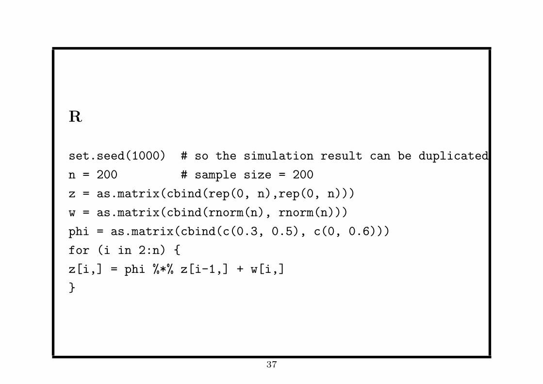
R

set.seed(1000) # so the simulation result can be duplicated

n = 200 # sample size = 200

z = as.matrix(cbind(rep(0, n),rep(0, n)))

w = as.matrix(cbind(rnorm(n), rnorm(n)))

phi = as.matrix(cbind(c(0.3, 0.5), c(0, 0.6)))

for (i in 2:n)

z[i,] = phi %*% z[i-1,] + w[i,]

37

Unit Root Test

In practice we always test unit roots for each series before running

VAR. The commands are

adf.test(z[,1], k = 1)

adf.test(z[,1], k = 4)

adf.test(z[,2], k = 1)

adf.test(z[,2], k = 4)

In this case, unit root is rejected (with p-value less than 0.05), so

VAR can be applied. If unit roots cannot be rejected then

1. Running VAR using differenced data if series are not cointegrated

2. Running Error Correction Model is series are cointegrated

38

Selecting the Lag Number p

In theory we should include sufficient lagged values so that the error

term is serially uncorrelated. In practice, we can choose p by

minimizing AIC

VARselect(z)

In this case, the VAR(1) has the smallest AIC -0.06176601, and so is

chosen.

39

Estimate VAR

var.1c = VAR(z, p=1, type = "both")

summary(var.1c)

var.1c = VAR(z, p=1, type = "none")

summary(var.1c)

1. We start with a VAR(1) with both intercept term and trend

term. Then we both terms are insignificant.

2. Next we run VAR(1) without intercept term or trend.

40

Result

The estimation result for y (the first series) is

Estimate Std.Error t value Pr(>|t|)

y1.l1 0.25493 0.06887 3.702 0.000278 ***

y2.l1 -0.05589 0.04771 -1.171 0.242875

1. ϕ11 = 0.25493, close to the true value 0.3

2. ϕ12 = −0.05589, and is insignificant

So the estimated regression for yt is

yt = 0.25493yt−1 − 0.05589xt−1

Exercise: find the estimated regression for xt

41

Equation-by-Equation OLS Estimation

We can get the same result by using these commands

y = z[,1]

ylag1 = c(NA, y[1:n-1])

x = z[,2]

xlag1 = c(NA, x[1:n-1])

eqy = lm(y~ylag1+xlag1-1) # without intercept

summary(eqy)

Exercise: What are the R commands that estimate the regression for

x (the second series)?

42

Variance-Covariance Matrix I

The true variance-covariance matrix (VCM) for the vector of error

terms are identity matrix

Ω = E(wtw′t) = E

ut

vt

(ut vt

) =

1 0

0 1

The estimated VCM is

Ω =

0.9104 −0.0391

−0.0391 0.9578

which is close to the true VCM.

43

Variance-Covariance Matrix II

To get Ω we need to keep the residuals and then compute two

variances and one covariance (with adjustment of degree of freedom)

sigmau2 = var(resy)*(n-1)/(n-2)

sigmav2 = var(resx)*(n-1)/(n-2)

sigmauv = cov(resy,resx)*(n-1)/(n-2)

omegahat = as.matrix(cbind(c(sigmau2, sigmauv), c(sigmauv, sigmav2)))

44

Cholesky Decomposition of Ω

The Cholesky Decomposition is

Ω = AA′

where A is lower triangular matrix. But the R function chol returns

A′ so we need to transpose it in order to get A :

A = (A′)′

The R commands are

Aprime = chol(omegahat)

A = t(Aprime)

The matrix A will be used to construct impulse response to

orthogonal (or structural form) errors

45

Impulse Response to Orthogonal Errors

The responses of y and x to the one-unit impulse of the orthogonal

(structural-form) the error for y can be obtained as

wtilde = as.matrix(c(1,0))

A1c = A%*%wtilde # or A1c = A[,1]

if1 = A1c

if2 = phihat%*%if1

if3 = phihat%*%if2

if4 = phihat%*%if3

46

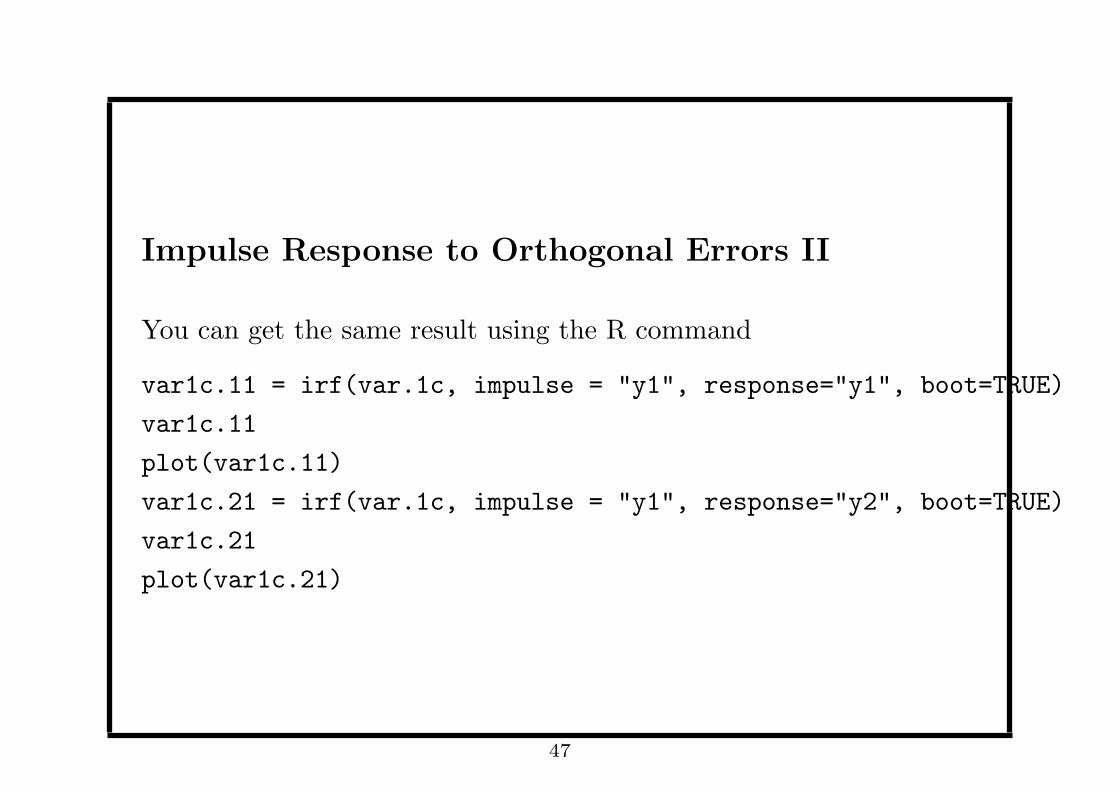
Impulse Response to Orthogonal Errors II

You can get the same result using the R command

var1c.11 = irf(var.1c, impulse = "y1", response="y1", boot=TRUE)

var1c.11

plot(var1c.11)

var1c.21 = irf(var.1c, impulse = "y1", response="y2", boot=TRUE)

var1c.21

plot(var1c.21)

47

Granger Causality Test

The R command is

causality(var.1c, cause = c("y2"))

causality(var.1c, cause = c("y1"))

The results are consistent with the DGP

Granger causality H0: y2 do not Granger-cause y1

F-Test = 1.372, df1 = 1, df2 = 394, p-value = 0.2422

Granger causality H0: y1 do not Granger-cause y2

F-Test = 69.3042, df1 = 1, df2 = 394, p-value = 1.443e-15

48