Lectures on Machine Learning (Fall 2017)

Hyeong In Choi Seoul National University

Lecture 9: Classification and Regression Tree

(CART)

(Draft: version 0.8.1)

Topics to be covered:

• Basic ideas of CART

• Classification tree

• Regression tree

• Impurity: entropy & Gini

• Node splitting

• Pruning

• Tree model selection (validation)

1 Introduction: basic ideas of CART

The Classification And Regression Tree (in short, CART) is a very pop-ular tree-based method that is in wide use. Its origin is in the so-calleddecision tree, but the version we present here adheres to a particular way ofconstructing trees. For example, CART always creates a binary tree, mean-ing each non-terminal node has two child nodes. This is in contrast with

1

general tree-based methods that may allow multiple child nodes. One bigappeal the tree-based method, and in particular CART, has is that the deci-sion process is very much akin to how we humans make decisions. Thereforeit is easy to understand and accept the results coming from the tree-styledecision process. This intuitive explanatory power is one big reason why thetree method will never go away. Another very appealing aspect of CARTis that, unlike many linear combination methods like logistic regression orsupport vector machine, it allows diverse types of input data. So the inputdata can mix numerical variables like price or area and categorical variableslike house type or location. This flexibility makes CART a favored tool ofchoice in a variety of applications. In this lecture we cover both the CARTclassification tree and the CART regression tree. The book by Breiman etal. [1] remains the best reference for CART.

1.1 Classification Tree

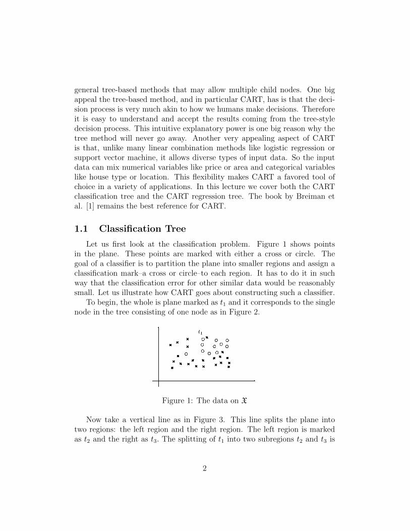
Let us first look at the classification problem. Figure 1 shows pointsin the plane. These points are marked with either a cross or circle. Thegoal of a classifier is to partition the plane into smaller regions and assign aclassification mark–a cross or circle–to each region. It has to do it in suchway that the classification error for other similar data would be reasonablysmall. Let us illustrate how CART goes about constructing such a classifier.

To begin, the whole is plane marked as t1 and it corresponds to the singlenode in the tree consisting of one node as in Figure 2.

Figure 1: The data on X

Now take a vertical line as in Figure 3. This line splits the plane intotwo regions: the left region and the right region. The left region is markedas t2 and the right as t3. The splitting of t1 into two subregions t2 and t3 is

2

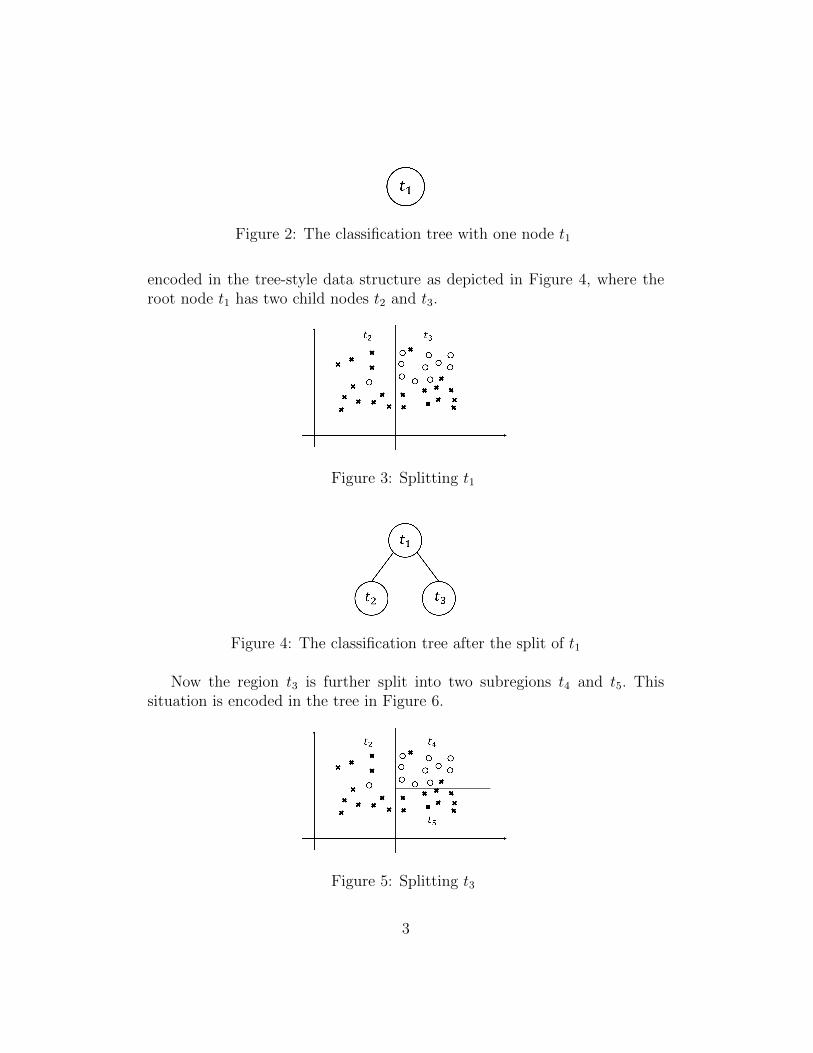
Figure 2: The classification tree with one node t1

encoded in the tree-style data structure as depicted in Figure 4, where theroot node t1 has two child nodes t2 and t3.

Figure 3: Splitting t1

Figure 4: The classification tree after the split of t1

Now the region t3 is further split into two subregions t4 and t5. Thissituation is encoded in the tree in Figure 6.

Figure 5: Splitting t3

3

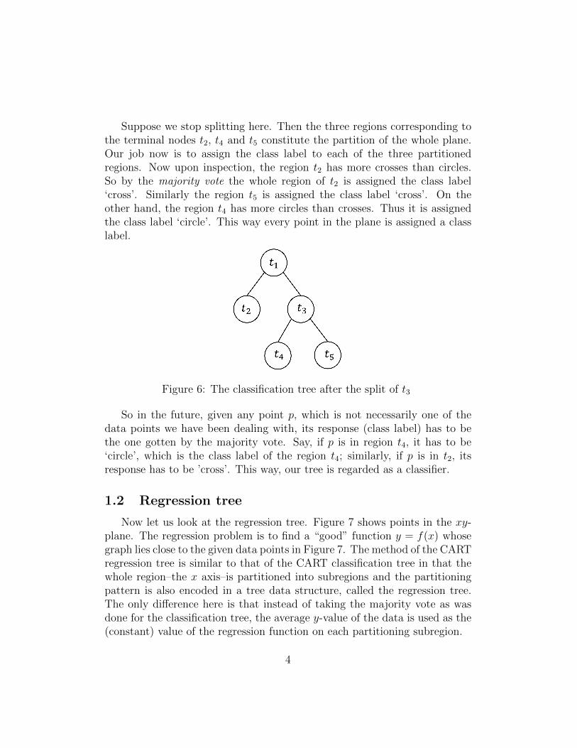
Suppose we stop splitting here. Then the three regions corresponding tothe terminal nodes t2, t4 and t5 constitute the partition of the whole plane.Our job now is to assign the class label to each of the three partitionedregions. Now upon inspection, the region t2 has more crosses than circles.So by the majority vote the whole region of t2 is assigned the class label‘cross’. Similarly the region t5 is assigned the class label ‘cross’. On theother hand, the region t4 has more circles than crosses. Thus it is assignedthe class label ‘circle’. This way every point in the plane is assigned a classlabel.

Figure 6: The classification tree after the split of t3

So in the future, given any point p, which is not necessarily one of thedata points we have been dealing with, its response (class label) has to bethe one gotten by the majority vote. Say, if p is in region t4, it has to be‘circle’, which is the class label of the region t4; similarly, if p is in t2, itsresponse has to be ’cross’. This way, our tree is regarded as a classifier.

1.2 Regression tree

Now let us look at the regression tree. Figure 7 shows points in the xy-plane. The regression problem is to find a “good” function y = f(x) whosegraph lies close to the given data points in Figure 7. The method of the CARTregression tree is similar to that of the CART classification tree in that thewhole region–the x axis–is partitioned into subregions and the partitioningpattern is also encoded in a tree data structure, called the regression tree.The only difference here is that instead of taking the majority vote as wasdone for the classification tree, the average y-value of the data is used as the(constant) value of the regression function on each partitioning subregion.

4

Figure 7: Given data with X on the x axis and Y on the y axis

Figure 8: The regression tree with one node t1

To start, Figure 7 has only one region: the entire x-axis. On this region,the regression function must be a constant function. So the most reasonablerepresentative has to be the average. This average y-value y1 is recorded inthe one-node tree in Figure 8.

Figure 9: Splitting t1

Figure 10: The regression tree after the split of t1

5

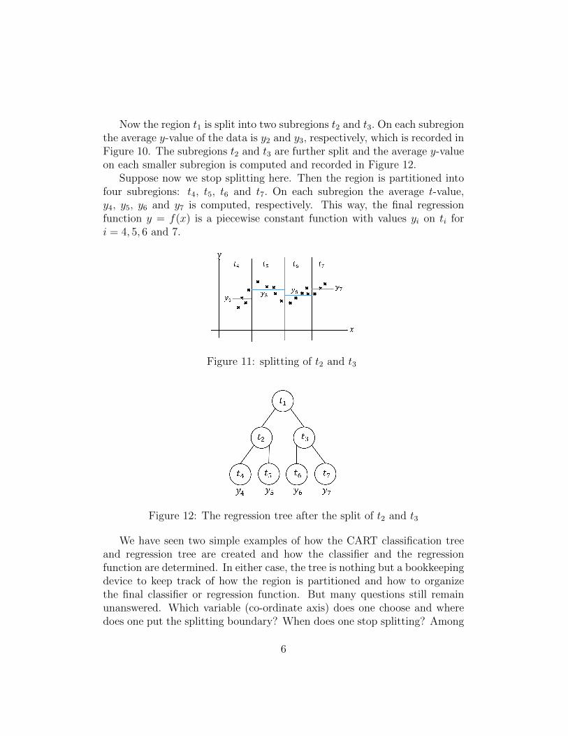
Now the region t1 is split into two subregions t2 and t3. On each subregionthe average y-value of the data is y2 and y3, respectively, which is recorded inFigure 10. The subregions t2 and t3 are further split and the average y-valueon each smaller subregion is computed and recorded in Figure 12.

Suppose now we stop splitting here. Then the region is partitioned intofour subregions: t4, t5, t6 and t7. On each subregion the average t-value,y4, y5, y6 and y7 is computed, respectively. This way, the final regressionfunction y = f(x) is a piecewise constant function with values yi on ti fori = 4, 5, 6 and 7.

Figure 11: splitting of t2 and t3

Figure 12: The regression tree after the split of t2 and t3

We have seen two simple examples of how the CART classification treeand regression tree are created and how the classifier and the regressionfunction are determined. In either case, the tree is nothing but a bookkeepingdevice to keep track of how the region is partitioned and how to organizethe final classifier or regression function. But many questions still remainunanswered. Which variable (co-ordinate axis) does one choose and wheredoes one put the splitting boundary? When does one stop splitting? Among

6

many possible candidates for the CART trees, which is the best? What is thetraining error and what is the reasonable expectation of the generalizationerror? These are all immediate questions to be answered and there are manyother issues to be clarified, which are the focus of the rest of this lecture.

2 Details of classification tree

Let us set up the basic notations we will be using in our subsequentdiscussion on classification tree. The data set is D = {(x(i), y(i))}Ni=1, wherex(i) ∈ X and y(i) ∈ Y, where Y = {1, · · · , K} is the set of K class labels. Wedefine the following empirical quantities:

N = |D|: the total number of data points

Nj = |{(x(i), y(i)) ∈ D : y(i) = j}|: the number of data points with classlabel j ∈ Y

Let t be a node, which is also identified with a subregion of X it represents.Then at t, we define

D(t) = {(x(i), y(i)) ∈ D : (x(i), y(i)) ∈ t}: the set of data points in thenode t

N(t) = |D(t)|: the number of data points in the node t

Nj(t) = |{(x(i), y(i)) ∈ D(t) : y(i) = j}|: the number of data points inthe node t with class label j ∈ Y

If one randomly chooses a data point from D, the probability of picking adata point with class label j should normally be Nj/N, if every point hasequal chance. In some case, however, this assumption of “equal chance” maynot be desirable. So in general we let π = (π(1), · · · , π(K)) be the priorprobability distribution of Y that represents the probability of picking theclass label j. Now define

p(j, t) = π(j)Nj(t)/Nj.

This is the probability of picking up a data point that is in t with the classlabel j. (Note that if π(j) = Nj/N, p(j, t) = Nj(t)/N.) Define

p(t) =∑j

p(j, t), (1)

7

which is the probability of picking a data point in the node t. We also define

p(j|t) = p(j, t)/p(t), (2)

which is the conditional probability of picking a data point with the classlabel j when the node t is given. Note that if π(j) = Nj/N, then p(t) =∑

j Nj(t)/N = N(t)/N and hence p(j|t) = Nj(t)/N(t). As we said above,CART has a particular way of creating a tree. First, it always splits alonga single feature (variable) of the input. Recall that the input vector x isof the form x = (x1, · · · , xd) where each xi can be a numeric, categorical(nominal), or discrete ordinal variable. (We also call it a co-ordinate or co-ordinate variable in this lecture.) At each node, CART always chooses one ofthose variables and splits the node based on the values of that variable only.In other words, CART does not combine variables like logistic regression does.Some tried to extend CART by combining variables, but the benefit weighedagainst the added complexity does not seem to justify the effort. Moreover,CART is not our ultimate tree-based method. In view of random forests wewill be covering in our next lecture, we prefer the simpler and faster approachof CART. Another particular way CART does splitting is that it alwayscreates two child nodes–hence the binary splitting–which results in a binarytree. Of course, general tree-based methods can split nodes into multiple(more than two) child nodes. But for CART, the split is always binary. Thereason is again simplicity as a single multiple split can be equivalently madeby several successive binary splits .

2.1 Impurity and splitting

In order to do the splitting, we need the following definitions.

Definition 1. An impurity function φ is a function φ(p1, · · · , pK) definedfor p1, · · · , pK with pi ≥ 0 for all i and p1 + · · ·+ pK = 1 such that

(i) φ(p1, · · · , pK) ≥ 0

(ii) φ(1/K, · · · , 1/K) is the maximum value of φ

(iii) φ(p1, · · · , pK) is symmetric with regard to p1, · · · , pK

(iv) φ(1, 0, · · · , 0) = φ(0, 1, · · · , 0) = φ(0, · · · , 0, 1) = 0.

The following are examples of impurity functions:

8

Example 1. (i) Entropy impurity

φ(p1, · · · , pK) = −∑i

pi log pi,

where we use the convention 0 log 0 = 0.

(ii) Gini impurity

φ(p1, · · · , pK) =1

2

∑i

pi(1− pi) =∑i<j

pipj

Definition 2. For node t, its impurity (measure) i(t) is defined as

i(t) = φ( p(1|t), · · · , p(K|t) ).

Splitting criterionGiven a node t, there are many possible ways of doing binary split. A generalprinciple is that it is better to choose the split that decreases the impuritythe most. Suppose t is split into tL and tR as in Figure 13. We define

Figure 13: tL and tR

pL = p(tL)/p(t) and pR = p(tR)/p(t) so that pL + pR = 1. Let us now see anexample on how impurity function is used to facilitate the “best” split. Theleft of Figure 14 denotes a node with four elements–two labeled with crossesand two with circles. The middle and the right figures represent two possibleways of splitting it.

The middle figure shows two child nodes t1 and t2. The entropy impurityof each child node is computed as:

t1 : p(◦|t1) = 0, p(×|t1) = 1

i(t1) = −{0 · log 0 + 1 · log 1} = 0

t2 : p(◦|t2) = 1 p(×|t2) = 0

i(t2) = −{1 · log 1 + 0 · log 0} = 0.

9

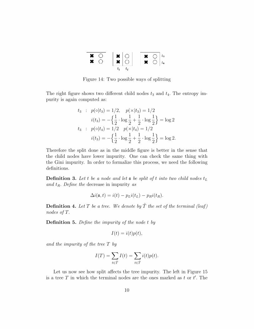
Figure 14: Two possible ways of splitting

The right figure shows two different child nodes t3 and t4. The entropy im-purity is again computed as:

t3 : p(◦|t3) = 1/2, p(×|t3) = 1/2

i(t3) = −{1

2· log

1

2+

1

2· log

1

2

}= log 2

t3 : p(◦|t4) = 1/2 p(×|t4) = 1/2

i(t3) = −{1

2· log

1

2+

1

2· log

1

2

}= log 2.

Therefore the split done as in the middle figure is better in the sense thatthe child nodes have lower impurity. One can check the same thing withthe Gini impurity. In order to formalize this process, we need the followingdefinitions.

Definition 3. Let t be a node and let s be split of t into two child nodes tLand tR. Define the decrease in impurity as

∆i(s, t) = i(t)− pLi(tL)− pRi(tR).

Definition 4. Let T be a tree. We denote by T the set of the terminal (leaf)nodes of T.

Definition 5. Define the impurity of the node t by

I(t) = i(t)p(t),

and the impurity of the tree T by

I(T ) =∑t∈T

I(t) =∑t∈T

i(t)p(t).

Let us now see how split affects the tree impurity. The left in Figure 15is a tree T in which the terminal nodes are the ones marked as t or t′. The

10

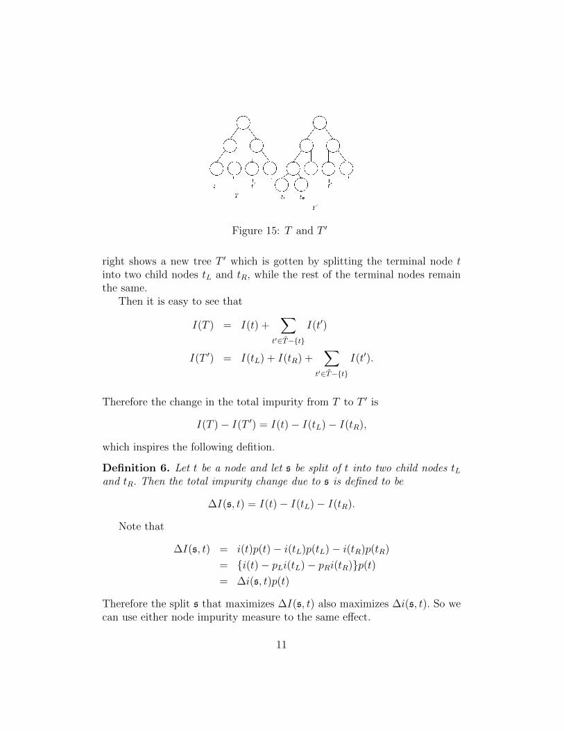
Figure 15: T and T ′

right shows a new tree T ′ which is gotten by splitting the terminal node tinto two child nodes tL and tR, while the rest of the terminal nodes remainthe same.

Then it is easy to see that

I(T ) = I(t) +∑

t′∈T−{t}

I(t′)

I(T ′) = I(tL) + I(tR) +∑

t′∈T−{t}

I(t′).

Therefore the change in the total impurity from T to T ′ is

I(T )− I(T ′) = I(t)− I(tL)− I(tR),

which inspires the following defition.

Definition 6. Let t be a node and let s be split of t into two child nodes tLand tR. Then the total impurity change due to s is defined to be

∆I(s, t) = I(t)− I(tL)− I(tR).

Note that

∆I(s, t) = i(t)p(t)− i(tL)p(tL)− i(tR)p(tR)

= {i(t)− pLi(tL)− pRi(tR)}p(t)= ∆i(s, t)p(t)

Therefore the split s that maximizes ∆I(s, t) also maximizes ∆i(s, t). So wecan use either node impurity measure to the same effect.

11

2.2 Determining node class label

Once a tree is fixed, a classifier can be defined from that tree. First,recall that every node of a tree corresponds to a subregion of X, and thusthe totality of the terminal nodes constitutes a partition of X into mutuallydisjoint subregions of X. The basic principle of classification using the treeis that the class label of such individual subregion should be determinedby majority vote. But the way we apply the majority vote is slightly moregeneral. Namely, instead of treating all misclassification cases with equalweights, we give different weight to each individual misclassification case byintroducing the following cost function.

Definition 7. Let i, j ∈ Y be labels. A cost C(i|j) of misclassifying classj as class i is defined as a nonnegative number satisfying C(j|j) = 0 for allj ∈ Y.

The simplest example of cost is C(i|j) = 1−δij, which simply says that themisclassification costs are the same regardless of the labels involved. Assumeour classifier declares the label of a node t to be i, while its “true” label isunknown. Then the expected cost of declaring the (response) label as i hasto be the weighted (in accordance with the probability p(j|t)) sum of cost,i.e., ∑

j

C(i|j)p(j|t). (3)

In particular, in case C(i|j) = 1 − δij, the expected cost of misclassificationis easily seen to be ∑

j

(1− δij)p(j|t) = 1− p(i|t). (4)

Definition 8. Let t be a node. The class label j∗(t) of t is defined to be

j∗(t) = argmini

∑j

C(i|j)p(j|t). (5)

In case there is a tie, tie breaking is done by some arbitrary rule.

In case C(i|j) = 1− δij, it is easily seen by (4) that

argmini

∑j

C(i|j)p(i|t) = argmaxi

p(i|t) (6)

12

Assume further that π(i) = Ni/N. Then we have p(i|t) = Ni(t)/N(t). Thusj∗(t) is reduced to

j∗(t) = argmaxi

Ni(t).

Namely in this case, the class label j∗(t) of t is determined by the simplemajority vote rule.

2.3 Misclassification cost

A goal of the classification tree is to minimize misclassification. A sim-plistic way of looking at this is to count the number of misclassified cases andcalculate the ratio. But a more general way is to utilize the misclassificationcost defined above. For that, we need the following definitions.

Definition 9. Define the misclassification cost r(t) of node t by

r(t) = mini

∑j

C(i|j)p(j|t). (7)

Let R(t) = r(t)p(t). Using this, define the misclassification cost R(T ) of treeT by

R(T ) =∑t∈T

R(t) =∑t∈T

r(t)p(t).

The following proposition shows that any split decreases the misclassifi-cation cost.

Proposition 1. Let a node t is split into tL and tR. Then

R(t) ≥ R(tL) +R(tR)

and the equality holds if j∗(t) = j∗(tL) = j∗(tR).

Proof. By (5),

r(t) =∑j

C(j∗(t)|j)p(j|t). (8)

Thus

R(t) = r(t)p(t) =∑j

C(j∗(t)|j)p(j|t)p(t)

=∑j

C(j∗(t)|j)p(j, t)

=∑j

C(j∗(t)|j){p(j, tL) + p(j, tR)}, (9)

13

where the last equality is due to the fact that Nj(t) = Nj(tL) +Nj(tR). Notethat for any node t, by (2) and (7), we have

R(t) = r(t)p(t) = mini

∑j

C(i|j)p(j, t).

Therefore, using this and (9), we have

R(t)−R(tL)−R(tR) =∑j

C(j∗(t)|j)p(j, tL)−mini

∑j

C(i|j)p(j, tL)

+∑j

C(j∗(t)|j)p(j, tR)−mini

∑j

C(i|j)p(j, tR) ≥ 0.

It is trivial to see that if j∗(t) = j∗(tL) = j∗(tR), then the equality holds.

2.4 Weakest-link cutting & minimal cost-complexitypruning

Proposition 1 above says that it is always better (not worse off) to keepsplitting all the way down. But then we may eventually get down to the pureterminal nodes that contain only one class. Such terminal node may evencontain only one point. But this must be an extreme case of overfitting. Sothe question arises as to when and how to stop splitting and on how to pruneback, if we have split too much. One quick rule of thumb is that one shouldstop splitting the node if the number of elements of the node is less than thepreset number. But still, the question remains:“What is the right-sized treeand how do we find such a tree that has a good generalization behavior?”This is the key issue we are addressing here. One way of preventing suchproblem is to penalize the tree if it has too many terminal nodes. It isakin to regularization we discussed in earlier lectures. For that, we need thefollowing definition.

Definition 10. Let α ≥ 0. For any node t, not necessarily a terminal node,define

Rα(t) = R(t) + α.

and for a tree T, define

Rα(T ) = R(T ) + α|T |,

where |T | is the number of terminal elements.

14

Now if we use Rα(t) as a new measure for (augmented) misclassificationcost, a split does not not necessarily decrease Rα(t), because it increasesα|T |. Thus this term acts like a regularization term and hopefully we maycome to a happy compromise.

Let us set up more notations. Let T be a given tree as in Figure 16. Lett2 be a node of T and let Tt2 be a new tree having t2 as the root node togetherwith all of its descendants in T. Tt2 is a subtree of T and is called a branch of

Figure 16: Given tree T

T at t2. This Tt2 is depicted in Figure 17. Suppose we cut off Tt2 from T. It

Figure 17: Subtree Tt2

means that we remove from T all the nodes of Tt2 except t2. The remainingtree, denoted by T −Tt2 , is depicted in Figure 18. Note that the node t2 stillremains intact in T −Tt2 . If we were to remove t2 from T −Tt2 , the subregionrepresented by t2 or its descendants disappear from the partition of X so that

15

Figure 18: Pruned subtree T − Tt2

the terminal nodes of the remaining tree would only be t6 and t7. But thenthe regions corresponding to t6 and t7 would not form the full set of X. If, onthe other hand, t2 is still intact in T −Tt2 as in Figure 18, the totality of thesubregions corresponding to the terminal nodes of T − Tt2 would still forma partition of X. That is the reason why we keep t2 in T − Tt2 . To formalizethis process, let us give the following definition.

Definition 11. A pruned subtree T1 of a tree T is a subtree obtained by thefollowing process:

(1) Take a node t of T

(2) Remove all descendants of t from T, but not t itself.

If T1 is a pruned subtree of T , we write T1 � T. Note in particular that T1always contains the root node of T. One should note the subtlety of definition:pruned subtree also has the same root note of the original tree, while subtreecan be any part of the original tree so that it may not necessarily contain theroot node of the original tree.

Suppose now we have done all the splitting and have grown a big treewhich is denoted by Tmax. We want to find a subtree of Tmax that minimizesRα. But there may be more than one such subtree. Thus to clear up theconfusion, we need the following definition.

Definition 12. Given a tree T and α ≥ 0, the optimally pruned subtree T (α)of T is defined by the following conditions:

(i) T (α) ≤ T

16

(ii) Rα(T (α)) ≤ Rα(T ′) for any pruned subtree T ′ � T.

(iii) If a pruned subtree T ′ � T satisfies the condition Rα(T (α)) = Rα(T ′),then T (α) � T ′

Proposition 2. T (α) exists and is unique.

Proof. Let T be a given tree with its root node t1. We use the induction onn = |T |. If n = 1, then T = {t1}, in which case there is nothing to prove.So we assume n > 1. Then there must be child nodes tL and tR of t1. LetTL be the subtree of T having tL as its root node together with all of itsdescendants. Similarly define TR. Thus TL = TtL and TR = TtR . TheseTL and TR, called the primary branches of T, are not pruned subtrees of T,because they do not contain the root node of the original tree.

Let T ′ be a nontrivial (having more than one node) pruned subtree ofT. Thus T ′ must contain the nodes t1, tL and tR of T. Let T ′L = T ′tL andT ′R = T ′tR be the primary branches of T ′. Then clearly T ′L is a pruned subtreeof TL having the same root node tL. Similarly, T ′R is a pruned subtree of TRhaving the same root node tR. (Note T ′L and T ′R are not pruned subtree of T.)By the induction hypothesis, there must be optimally pruned subtrees TL(α)and TR(α) of TL and TR, respectively. There are two cases to consider.

The first to consider is the case in which

Rα(t1) ≤ Rα(TL(α)) +Rα(TR(α)). (10)

Then by the definition of TL(α), we must have Rα(TL(α)) ≤ Rα(T ′L), andsimilarly, Rα(TR(α)) ≤ Rα(T ′R). Since Rα(T ′) = Rα(T ′L)+Rα(T ′R), combiningthis with (10), we then have

Rα(t1) ≤ Rα(T ′).

Since this is true for any pruned subtree T ′ of T, we can conclude thatT (α) = {t1}.

The remaining case is the one in which

Rα(t1) > Rα(TL(α)) +Rα(TR(α)). (11)

Now create a new tree T1 by joining TL(α) and TR(α) to t1. Then clearly T1is a pruned subtree of T and TL(α) and TR(α) are the primary branches ofT1. Clearly

Rα(T1) = Rα(TL(α)) +Rα(TR(α)). (12)

17

Now by (11), T (α), if it ever exists, cannot be {t1}. So now let T ′ beany nontrivial pruned subtree of T. Then by the definition of TL(α), we haveRα(TL(α)) ≤ Rα(T ′L), and similarly, Rα(TR(α)) ≤ Rα(T ′R). Since Rα(T ′) =Rα(T ′L) +Rα(T ′R), combining this with (12), we then must have

Rα(T1) ≤ Rα(T ′).

Therefore T1 is the pruned subtree of T that has the smallest Rα-value amongall pruned subtrees of T.

It remains to show that any strictly smaller pruned subtree of T1 haslarger Rα-value. So let T ′ be a strictly smaller pruned subtree of T1. Wemay assume without loss of generality T ′L < TL(α) and T ′R ≤ TR(α). Thenagain, by the definition of TL(α), we have Rα(TL(α)) < Rα(T ′L), and similarlyRα(TR(α)) ≤ Rα(T ′R). Then using the same argument as above, we have

Rα(T1) < Rα(T ′).

Therefore we can conclude that

T1 = T (α).

Let us now embark on the pruning process. The first thing to do is tocome up with the smallest subtree T (0) with the cost R0 = R. Let us seehow we do it. Start with Tmax. Suppose tL and tR are terminal nodes withthe same parent t. By Proposition 1, R(t) ≥ R(tL) +R(tR). If, furthermore,R(t) = R(tL) + R(tR), then prune at t. And repeat this process to get asmallest T1 ≤ Tmax with R(T1) = R(Tmax). Note that T1 is easily seen to beequal to T (0). Also ,the following proposition easily follows from the way T1is constructed.

Proposition 3. For any non-terminal node t ∈ T1 = T (0),

R(Tt) < R(t).

The next step is to find T (α). But the trouble is that there are so manypossibilities for α. Let us see how to come up with such “good” α.

Proposition 3, by the continuity argument, easily implies that for α issufficiently small,

Rα(Tt) < Rα(t), (13)

18

at any node t ∈ T (0). In that case, we’d be better off not pruning. Note that

Rα(t) = R(t) + α

Rα(Tt) = R(Tt) + α|Tt|.

Therefore (13) is equivalent to saying that

α <R(t)−R(Tt)

|Tt| − 1. (14)

But as α gets larger, there appears a node (or nodes) at which (14) is nolonger valid. To find such node(s), let us define a function g1(t) of node t by

g1(t) =

R(t)−R(Tt)

|Tt| − 1if t /∈ T1

∞ else.

Defineα2 = min

t∈T1g1(t).

So for α < α2, there is no node at which (14) is violated. But for α = α2,there is at least one node at which the inequality (14) becomes the equality.Such nodes are called weakest-link nodes. Suppose t′1 is such node. Then

g1(t′1) = α2 = min

t∈T1g1(t).

We then prune T1 at t′1 to come up with a pruned subtree T1−Tt′ . Note thatRα2(Tt′) = Rα2(t

′). Therefore

Rα2(T1) = Rα2(T1 − Tt′).

There may be more than one such weakest-link nodes. Suppose there are twosuch nodes. If one of them is an ancestor of the other, prune at the ancestor(then its descendants are all gone). If neither one is an ancestor of the other,prune at both. Keep doing this for all such weakest-link nodes. This way,we get a new subtree T2 and it is not hard to see that

T2 = T (α2).

19

Using T2 in lieu of T1, we can repeat the same process to come up with α3

and T3 = T (α3). Repeat this process until we arrive at the subtree with theroot node only. Namely, we get the following sequence of pruned subtrees.

T1 ≥ T2 ≥ · · · ≥ {t1}, (15)

where Tk = T (αk) and0 = α1 < α2 < · · · .

We need the following proposition for cross validation.

Proposition 4. (i) If α1 ≤ α2, then T (α2) ≤ T (α1)

(ii) For α with αk ≤ α < αk+1, T (αk) = T (α)

Proof. Proof of (i): The proof is based on induction on |T |. Recall that theproof of Proposition 2 shows that T (α) is either {t1} or the join of TL(α) andTR(α) at t1. Suppose T (α1) = {t1}, i.e.,

Rα(t1) ≤ Rα(T ′), (16)

for any pruned subtree T ′ of T. Then

Rα2(t1) = Rα1(t1) + α2 − α1

≤ Rα1(T′) + α2 − α1

≤ Rα1(T′) + (α2 − α1)|T ′|

= Rα2(T′),

where the first inequality above is due to (16). Therefore we can easilyconclude that T (α2) = {t1}.

Assume now T (α1) is nontrivial and is the join of TL(α1) and TR(α1) att1. By the induction hypothesis, we may assume that TL(α2) ≤ TL(α1) andTR(α2) ≤ TR(α1). Thus if T (α2) is the join of TL(α2) and TR(α2) at t1, theproof of (i) is complete. On the other hand, if T (α2) = {t1}, then again it isobvious that {t1} is a pruned subtree of anything.

Proof of (ii): Suppose the assertion of (ii) is false. Then (i) says thatT (α) < T (αk). Therefore the pruning of T (αk) must have occurred at somenode, say, at t′ ∈ T (αk). Let T (αk)t′ be the branch of T (αk) at t′. Namely,T (αk)t′ is the subtree of T (αk) with t′ as its root node together with all ofits descendant nodes in T (αk). Since the pruning has occurred at t′, we musthave Rα(t′) ≤ Rα(T (αk)t′). It is then not hard to see that αk+1 ≤ α. This isa contradiction to the assumption of (ii).

20

2.5 Model selection (validation)

Once the subtrees are found as in (15), our next job is to determine whichone is the “best” subtree. It is really a model selection problem. As usual,there are two ways to do it: testing and cross validation.

Before we embark on the model selection task, let us review the underlyingprobability model. Recall the nature of data set D = {(xi, yi)}ni=1. The datapoint (xi, yi) is gotten as a random IID sample of the random variable (X, Y )drawn from the distribution PX,Y . It is denoted in our usual notation by(X, Y ) ∼ PX,Y . Let us now fix a tree T. Then T gives rise to a classifier f asexplained in Definition 8 and the discussion following it.

With f and the probability P = PX,Y , we can define the following quan-tities. Note that they depend only on P not on any particular data set D.In this sense, we call them theoretical quantities associated with f or equiv-alently with T.

(i) Q∗(i|j) = P (f(x) = i|Y = j): the theoretical probability of classifyingclass j as being class i

(ii) R∗(j) =∑

iC(i|j)Q∗(i|j): the theoretical expected misclassificationcost of the class j

(iii) R∗(f) = R∗(T ) =∑

j R∗(j)π(j): the overall theoretical expected cost

of the classifier f

Note that in case C(i|j) = 1− δij, R∗(f) is nothing but the misclassification

21

probability. Namely,

R∗(f) =∑j

R∗(j)π(j)

=∑j

∑i

C(i|j)Q∗(i|j)π(j)

=∑j

∑i

(1− δij)Q∗(i|j)π(j)

=∑j

∑i

Q∗(i|j)π(j)−∑i

Q∗(i|i)π(i)

= 1−∑i

Q∗(i|i)π(i)

=∑i

{1−Q∗(i|i)}π(i)

=∑i

P (f(X) 6= Y |Y = i)π(i)

= P (f(X) 6= Y ).

Method A: Using separate training and testing setsDivide D into disjoint training set D(1) and testing set D(2). So

D = D(1) ∪D(2).

Use D(1) to constructT1 ≥ T2 ≥ · · · ≥ {t1}.

as in (15). Then use D(2) for testing and selecting the best model (Tk).Now each Tk defines the classifier fk. With it, define the following quan-

tities: Let N(2)j be the number of data points in D(2) with class label j and

N(2)ij (k) the number of data points in D(2) with class label j that is classified

by fk as class i. Define the estimator Qtsk (i|j) for Q∗(i|j) by

Qtsk (i|j) = N

(2)ij (k)/N

(2)j .

Here, ‘ts’ stands for “test sample.” If N(2)j = 0, we set Qts

k (i|j) = 0. Similarlydefine the estimators Rts

k (j) and Rts(Tk) for R∗(j) and R∗(Tk), respectively

22

by

Rtsk (j) =

∑i

C(i|j)Qtsk (i|j)

Rts(Tk) =∑j

Rtsk (j)π(j).

This way, the overall expected cost Rts(Tk) of the classifier fk is obtained foreach k. We then choose Tk′ with the smallest overall expected cost. Namely,

Rts(Tk′) = minkRts(Tk).

Method B: Cross validationAs is the standard practice in the V-fold cross validation, divide D into Vequal (as nearly as possible) disjoint sets D1, · · · ,DV and Let D(v) = D−Dv,for v = 1, · · · , V. We first grow Tmax using D and get 0 = α1 < α2 < · · · and

T1 ≥ T2 ≥ · · · ≥ {t1},

where Tk = T (αk) Now these trees T1, T2, · · · cannot be used for cross vali-dation because the data in the cross validation sets Dv were already used toconstruct them, hence tainted. Now define

α′k =√αkαk+1.

For each v ∈ {1, 2, · · · , V } and α ∈ {α′1, α′2, · · · }, use D(v) to grow T(v)max and

then find T (v)(α) by applying the usual pruning process using Rα. Since Dv

is not used in the construction of T (v)(α), it can be used as a cross validationset. So put down Dv through T (v)(α) to compute the following quantities

• N (v)ij : the number of class j in Dv classified by T (v)(α) as i

• Nij =∑

vN(v)ij : the total number of class j that are classified as i in

the cross validation process

The idea is that for large V, T (v)(α) and T (α) have very similar accuracy.Thus we can define the following estimates. In here, the symbol ∼ denotes

23

that the left of it is an estimator of the quantity in the right.

Qcv(i|j) = Nij/N ∼ Q∗(i|j)Rcv(j) =

∑i

C(i|j)Qcv(i|j) ∼ R∗(j)

Rcv(T (α)) =∑j

Rcv(j)π(j) ∼ R∗(T (α)).

Now by Proposition 4, Tαk′= Tαk

= Tk. Therefore we get the estimates forRcv(Tk) by

Rcv(Tk) = Rcv(Tαk).

Finally, choose Tk′ among T1, T2, · · · , {t1} such that

Rcv(Tk′) = minkRcv(Tk).

Figure 19: α′k

3 Details of regression tree

We now look at the regression tree. The data is D = {(x(i), y(i))}Ni=1,where x(i) ∈ X and y(i) ∈ Y. Typically X = Rd and Y = RK . The goal ofregression tree algorithm is to construct a function f : X→ Y such that theerror ∑

i

|f(x(i))− y(i)|2

is small. The way to do it is to construct a tree and define a constant valueon each subregion corresponding to the terminal node of the tree. Thus fconstructed this way is a piecewise constant function.

Recall the way we construct a tree. In particular, any node t ∈ T corre-sponds to a subset of X. On each node t, define the average y-value y(t) ofthe data on the node t by

y(t) =1

N(t)

∑x(i)∈t

y(i),

24

which is an estimator of E[Y |X ∈ t]. We also define the (squared) error rater(t) of node t by

r(t) =1

N(t)

∑x(i)∈t

(y(i) − y(t))2.

It is nothing but the variance of the node t, which is also an estimator of

Var(Y |X ∈ t) = σ2(Y |X ∈ t).

We define the cost R(t) of the node t by

R(t) = r(t)p(t).

Recall that p(t) =N(t)

N. Therefore

R(t) =1

N

∑x(i)∈t

(y(i) − y(t))2.

We need the following proposition.

Proposition 5. Suppose a node t is split into tL and tR. Then

R(t) ≥ R(tL) +R(tR).

The equality holds if and only if y(t) = y(tL) = y(tR).

Proof.

R(t) =1

N

∑x(i)∈t

(y(i) − y(t))2

=1

N

∑x(i)∈tL

(y(i) − y(t))2 +1

N

∑x(i)∈tR

(y(i) − y(t))2

≥ 1

N

∑x(i)∈tL

(y(i) − y(tL))2 +1

N

∑x(i)∈tR

(y(i) − y(tR))2,

where the last inequality is due to following Lemma 1. The statement on theequality also follows from Lemma 1.

25

Lemma 1.y(t) = argmin

a

∑x(i)∈t

(y(i) − a)2.

i.e., ∑x(i)∈t

(y(i) − y(t))2 ≤∑x(i)∈t

(y(i) − a)2.

for all a ∈ R and “=” holds if and only if a = y(t).

Proof.∑x(i)∈t

(y(i) − a)2 =∑x(i)∈t

(y(i) − y(t) + y(t)− a)2

=∑x(i)∈t

(y(i) − y(t))2 − 2(y(t)− a)∑x(i)∈t

(y(i) − y(t)) +N(t)(y(t)− a)2

=∑x(i)∈t

(y(i) − y(t))2 +N(t)(y(t)− a)2

≥∑x(i)∈t

(y(i) − y(t))2

Clearly the equality holds if and only if y(t)− a = 0.

Let s be a split of a node t. Define the decrease ∆R(s, t) of the cost by sas

∆R(s, t) = R(t)−R(tL)−R(tR).

The splitting rule at t is s∗ such that we take the split s∗ among all possiblecandidate splits that decreases the cost most. Namely,

∆R(s∗, t) = maxs

∆R(s, t).

Remark. One may use this splitting rule for the split of classification tree.

This way, we can grow the regression tree to Tmax. As before, one quickrule of thumb is that one stops splitting the node if the number of elementsof the node is less than the preset number. Once Tmax is found, we can pruneback. The pruning method for the regression tree is exactly the same for theclassification tree except that we define Rts(T ) and Rcv(T ) differently.

26

For the test sample method, divide D = D(1) ∪ D(2), and use D(1) forconstructing the tree and D(2) for testing. Define

Rts(T ) =1

|D(2)|∑

(x(i),y(i))∈D(2)

(y(i) − y(τ(x(i))))2,

where τ is the map τ : X → T such that τ(x) is the terminal node thatcontains x. As was done in the case of classification tree, this Rts(T ) is usedfor choosing the best tree.

For the cross-validation method, use the division D = D1 ∪ · · · ∪DV andfor each v use D(v) = D−Dv for constructing the tree T (v), and Dv for crossvalidation. Define

Rcv(T ) =1

V

V∑v=1

∑(x(i),y(i))∈Dv

(y(i) − y(v)(τ (v)(x(i)))),

where τ (v) : X → T (v) is the map such that τ (v)(x) is the terminal node ofT (v) containing x, and y(v) is gotten using D −Dv as the training set. Therest of the cross validation is routine.

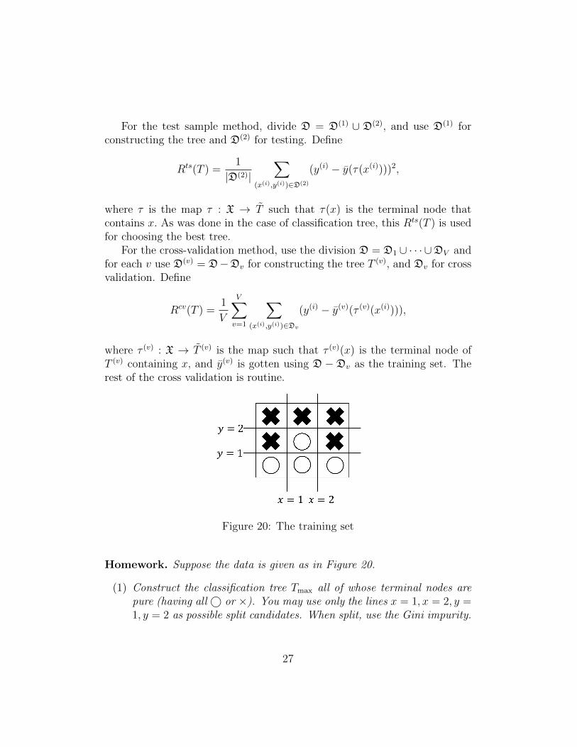
Figure 20: The training set

Homework. Suppose the data is given as in Figure 20.

(1) Construct the classification tree Tmax all of whose terminal nodes arepure (having all© or ×). You may use only the lines x = 1, x = 2, y =1, y = 2 as possible split candidates. When split, use the Gini impurity.

27

(2) Prune Tmax using the weakest-link cut to come up with a sequence ofsubtrees:

T1 ≥ T2 ≥ · · · ≥ {root}.

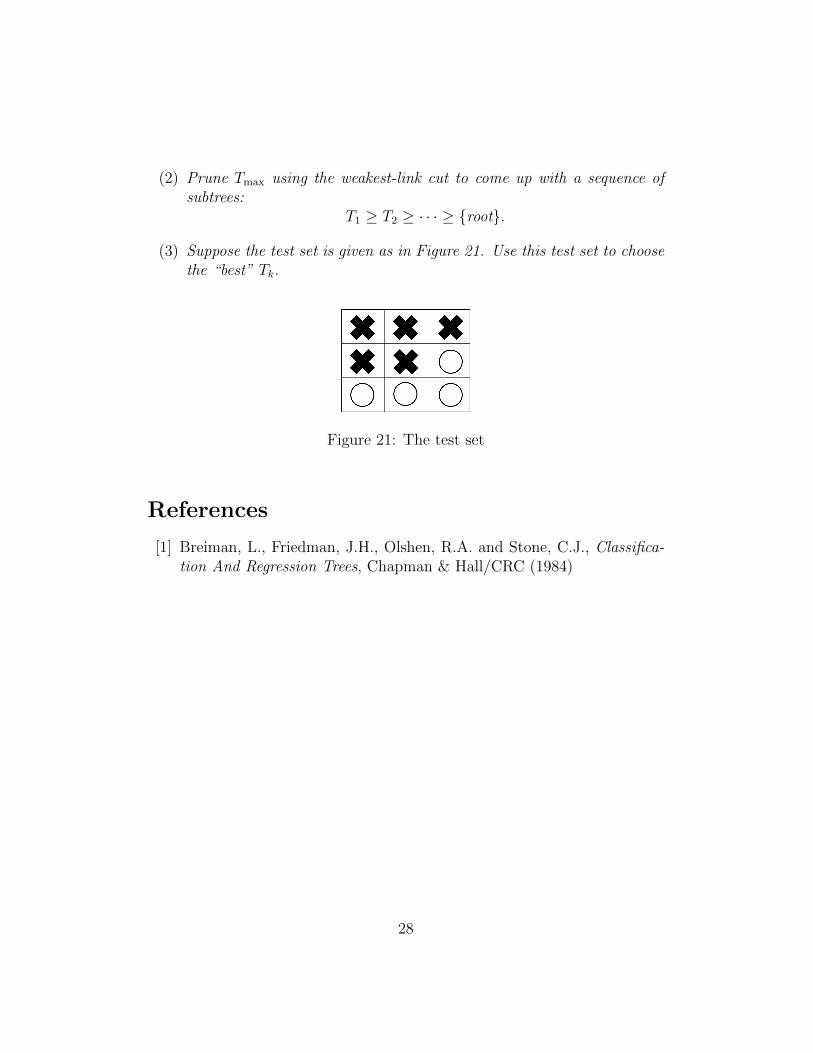
(3) Suppose the test set is given as in Figure 21. Use this test set to choosethe “best” Tk.

Figure 21: The test set

References

[1] Breiman, L., Friedman, J.H., Olshen, R.A. and Stone, C.J., Classifica-tion And Regression Trees, Chapman & Hall/CRC (1984)

28