lecture – 9 conversion between state space and … 10.pdflecture – 9 conversion between state...

Lecture – 9

Conversion Between State Space and Transfer Function Representations in

Linear Systems – I

Dr. Radhakant PadhiAsst. Professor

Dept. of Aerospace EngineeringIndian Institute of Science - Bangalore

ADVANCED CONTROL SYSTEM DESIGN Dr. Radhakant Padhi, AE Dept., IISc-Bangalore

2

State Space Representation(noise free linear systems)

State Space form

Transfer Function form

A - System matrix- n x n

- Input matrix- n x m

- Output matrix- p x n

- Feed forward matrix – p x m

BCD

X AX BUY CX DU= += +

Q: Is conversion betweenthe two forms possible?

A: Yes.


3

Deriving Transfer Function Model From Linear State Space Model

Known:

Taking Laplace transform (with zero initial conditions)

X AX BUY CX DU= += +

( ) ( ) ( )( ) ( ) ( )

sX s AX s BU sY s CX s DU s

= += +


4

Deriving Transfer functions from State Space Description

The state equation can be placed in the form

Pre-multiplying both sides by

Substituting for X (s) in the output equation,

1)( −− AsI

1

Transfer Function Matrix ( )

( ) ( ) ( )T s

Y s C sI A B D U s−⎡ ⎤= − +⎣ ⎦

)()()( sBUsXAsI =−

)()()( 1 sBUAsIsX −−=


5

ExampleState space model

Using the expression for derived transfer function

[ ] [ ]

1 1

2 2

1

2

0 1 02 3 1

1 0 0

BA

C D

x xu

x x

xy u

x

⎡ ⎤ ⎡ ⎤⎡ ⎤ ⎡ ⎤= +⎢ ⎥ ⎢ ⎥⎢ ⎥ ⎢ ⎥− −⎣ ⎦ ⎣ ⎦⎣ ⎦ ⎣ ⎦

⎡ ⎤= +⎢ ⎥

⎣ ⎦

)2)(1(1

231

)()(

2 ++=

++=

sssssUsY


6

Example: Detail Algebra( ) ( )

[ ] [ ]

[ ]

[ ] ( )

[ ]

1

1

1

2 2

0 0 1 01 0 0

0 2 3 1

1 01 0

2 3 1

3 1 011 02 13 2

11 11 03 2 3 2

T s C sI A B D

ss

ss

sss s

ss s s s

−

−

−

= − +

⎛ ⎞⎡ ⎤ ⎡ ⎤ ⎡ ⎤= − +⎜ ⎟⎢ ⎥ ⎢ ⎥ ⎢ ⎥− −⎣ ⎦ ⎣ ⎦ ⎣ ⎦⎝ ⎠

−⎡ ⎤ ⎡ ⎤= ⎢ ⎥ ⎢ ⎥+⎣ ⎦ ⎣ ⎦

⎛ ⎞ +⎡ ⎤ ⎡ ⎤= ⎜ ⎟ ⎢ ⎥ ⎢ ⎥⎜ ⎟ −+ + ⎣ ⎦ ⎣ ⎦⎝ ⎠

⎡ ⎤= =⎢ ⎥+ + + +⎣ ⎦


7

Deriving State Space Model From Transfer Function Model

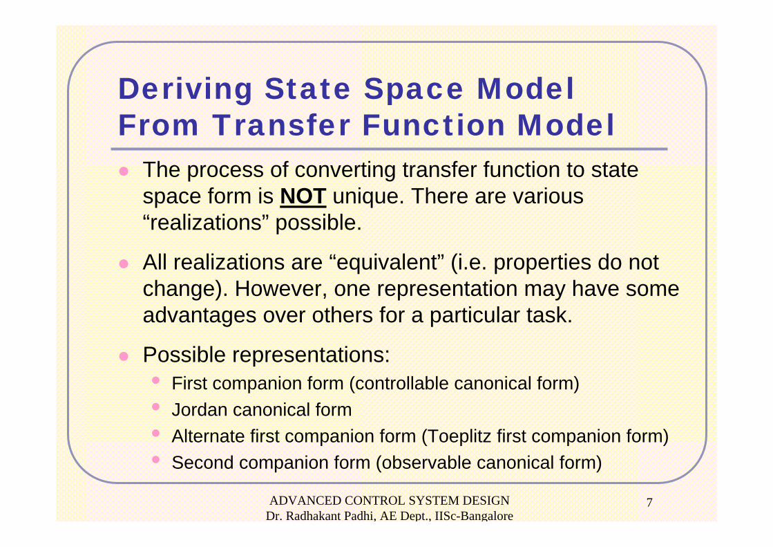
The process of converting transfer function to state space form is NOT unique. There are various “realizations” possible.

All realizations are “equivalent” (i.e. properties do not change). However, one representation may have some advantages over others for a particular task.

Possible representations:• First companion form (controllable canonical form)• Jordan canonical form• Alternate first companion form (Toeplitz first companion form)• Second companion form (observable canonical form)


8

First Companion Form: SISO Case(Controllable canonical form)

( ) ( )

11 1

11 1

1

1 1

( ) 1( )( ) n n

n n

n nn n

n n

nn n

y sH su s s a s a s a

y a y a y a y u

d y d ya a y udt d t

−−

−−

−

−

⎡ ⎤= = ⎢ ⎥+ + + +⎣ ⎦

+ + + + =

+ + + =


9

11

22

2 2

1

1

Choose output ( ) and its ( 1) derivatives as

differentiating

nn

n nn n

y t ndyxx ydt

dyx d yxdt dt

d yx d yxdt dt

−

−

−

⎡ ⎤==⎡ ⎤ ⎢ ⎥⎢ ⎥ ⎢ ⎥⎢ ⎥= ⎢ ⎥=⎢ ⎥ ⎢ ⎥⎯⎯→ ⎯⎯→⎢ ⎥ ⎢ ⎥⎢ ⎥ ⎢ ⎥⎢ ⎥ ⎢ ⎥=⎢ ⎥ ⎢ ⎥=⎣ ⎦

⎣ ⎦



10

[ ]

1 1

2 2

3 3

1 1

1 2 1

1

2

3

1

0 1 0 0 0 0 0 00 0 1 0 0 0 0 00 0 0 1 0 0 0 0

00 0 0 0 0 0 0 1 0

1

1 0 0 0

n n

n n n n n

n

x xx xx x

u

x xx a a a a x

xxx

y

xx

− −

− −

−

⎡ ⎤ ⎡ ⎤ ⎡ ⎤ ⎡ ⎤⎢ ⎥ ⎢ ⎥ ⎢ ⎥ ⎢ ⎥⎢ ⎥ ⎢ ⎥ ⎢ ⎥ ⎢ ⎥⎢ ⎥ ⎢ ⎥ ⎢ ⎥ ⎢ ⎥

= +⎢ ⎥ ⎢ ⎥ ⎢ ⎥ ⎢ ⎥⎢ ⎥ ⎢ ⎥ ⎢ ⎥ ⎢ ⎥⎢ ⎥ ⎢ ⎥ ⎢ ⎥ ⎢ ⎥⎢ ⎥ ⎢ ⎥ ⎢ ⎥ ⎢ ⎥

− − − − ⎢ ⎥⎢ ⎥ ⎢ ⎥ ⎢ ⎥ ⎣ ⎦⎣ ⎦ ⎣ ⎦ ⎣ ⎦

= [ ]0

n

u

⎡ ⎤⎢ ⎥⎢ ⎥⎢ ⎥

+⎢ ⎥⎢ ⎥⎢ ⎥⎢ ⎥⎢ ⎥⎣ ⎦



11

n integrators

First Companion Form: SISO Case(Controllable canonical form): Block Diagram


12

Example:(Constant in the Numerator)

2

3 2

( ) 7 2( )( ) 9 26 24

C s s sT sR s s s s

+ += =

+ + +

3 2

1 2 3

1 2

2 3

3 1 2 3

1

( 9 2 6 2 4 ) ( ) 2 4 ( )w ith ze ro in itia l co n d itio n s

9 2 6 2 4 2 4L et , ,

2 4 2 6 9 2 4

s s s C s R s

c c c c rx c x c x c

x xx xx x x x ry c x

+ + + =

+ + + =

==

= − − − += =

3 integrators


13

Example:(Polynomial in the Numerator)

3 21

1 2

2 3

3 1 2 3

21

3 2 1

For the block containing denominator( 9 26 24) ( ) 24 ( )

24 26 9For Numerator Block

( ) ( 7 2) ( )Taking inverse Laplace transform

7 2

s s s X s R sx xx xx x x x r

C s s s X s

y x x x

+ + + ===

= − − − +

= + +

= + +


14

Example With A Polynomial In The Numerator

3 integrators


15

Systems Having Single Input but Multiple Outputs

Generalization of the concepts discussed to this case is straight forward:

A and B matrices remain same

C and D matrices get modified


16

Example

11 2

22 2

( ) 2 3( ) and ( ) 3 4 5( ) 3 2( )( ) 3 4 5

y s sH su s s sy s sH su s s s

+= =

+ ++

= =+ +

( )1 11 2

( ) ( )( ) 1( ) 2 3( ) ( ) ( ) 3 4 5

y s y sz sH s su s u s z s s s

⎛ ⎞⎛ ⎞ ⎛ ⎞= = = +⎜ ⎟⎜ ⎟ ⎜ ⎟+ +⎝ ⎠⎝ ⎠⎝ ⎠


17

Example – contd.

uxx

xx

⎥⎦

⎤⎢⎣

⎡+⎥

⎦

⎤⎢⎣

⎡⎥⎦

⎤⎢⎣

⎡−−

=⎥⎦

⎤⎢⎣

⎡31

03435

10

2

1

2

1

[ ] [ ]uxx

y

xxzzy

023

3232

2

1

1

121

+⎥⎦

⎤⎢⎣

⎡=

+=+=

1 24 5 1 Define ,3 3 3

z z z u x z x z+ + =


18

Example – contd.

( )22 2

( )( ) 1( ) 3 2( ) ( ) 3 4 5

y sz sH s su s z s s s

⎛ ⎞⎛ ⎞ ⎛ ⎞= = +⎜ ⎟⎜ ⎟ ⎜ ⎟+ +⎝ ⎠⎝ ⎠⎝ ⎠

[ ] [ ]

2 2 1

12

2

and are the same3 2 3 2

2 3 0

A By z z x x

xy u

x

= + = +

⎡ ⎤= +⎢ ⎥

⎣ ⎦

Note: Block diagram representation is fairly straight forward.The realization requires n integrators.


19

Jordan Canonical Form(Non-repeated roots)

[ ]

1 20

1 2

0

10

( )( )( )

All the poles of the transfer function are distinct, i.e. no repeated poles 's are called "residues" of the reduced transfer function ( )

( )( ) ( )

n

n

i

rr ry sH s du s s s s

r H s bru sy s d u s

λ λ λ= = + + + +

− − −

−

= + 2

1 2

11 1 1 1 1

1

( )( )

Let( )( )

( )( )

n

n

nn n n n n

n

r u sr u ss s s

ru sx s x x rus

r u sx s x x r us

λ λ λ

λλ

λλ

+ + +− − −

⎡ ⎤= − =⎡ ⎤⎢ ⎥− ⎢ ⎥⎢ ⎥⎢ ⎥⎢ ⎥ →⎢ ⎥⎢ ⎥⎢ ⎥⎢ ⎥= − =⎣ ⎦⎢ ⎥−⎣ ⎦


20

Jordan Canonical Form(Non-repeated roots)

[ ] [ ]

1 1 1 1

2 2 2 2

1

20

0 00 00 00 0

1 1 1

n n n n

n

x x rx x r

u

x x r

xx

y d u

x

λλ

λ

⎡ ⎤ ⎡ ⎤ ⎡ ⎤ ⎡ ⎤⎢ ⎥ ⎢ ⎥ ⎢ ⎥ ⎢ ⎥⎢ ⎥ ⎢ ⎥ ⎢ ⎥ ⎢ ⎥= +⎢ ⎥ ⎢ ⎥ ⎢ ⎥ ⎢ ⎥⎢ ⎥ ⎢ ⎥ ⎢ ⎥ ⎢ ⎥⎣ ⎦ ⎣ ⎦ ⎣ ⎦ ⎣ ⎦

⎡ ⎤⎢ ⎥⎢ ⎥= +⎢ ⎥⎢ ⎥⎣ ⎦


21

Jordan Canonical Form(Non-repeated roots): Block Diagram


22

Jordan Canonical Form: Example(Non-repeated roots)

Given

By partial fraction,

Define two transfer functions

( ) 1( ) ( 1)( 2)

y su s s s

=+ +1 1( ) ( )

1 2y s u s

s s⎡ ⎤= −⎢ ⎥+ +⎣ ⎦

1 21 1( ) ( ) , ( ) ( )

1 2x s u s x s u s

s s= =

+ +


23

Jordan Canonical Form: Example(Non-repeated roots)

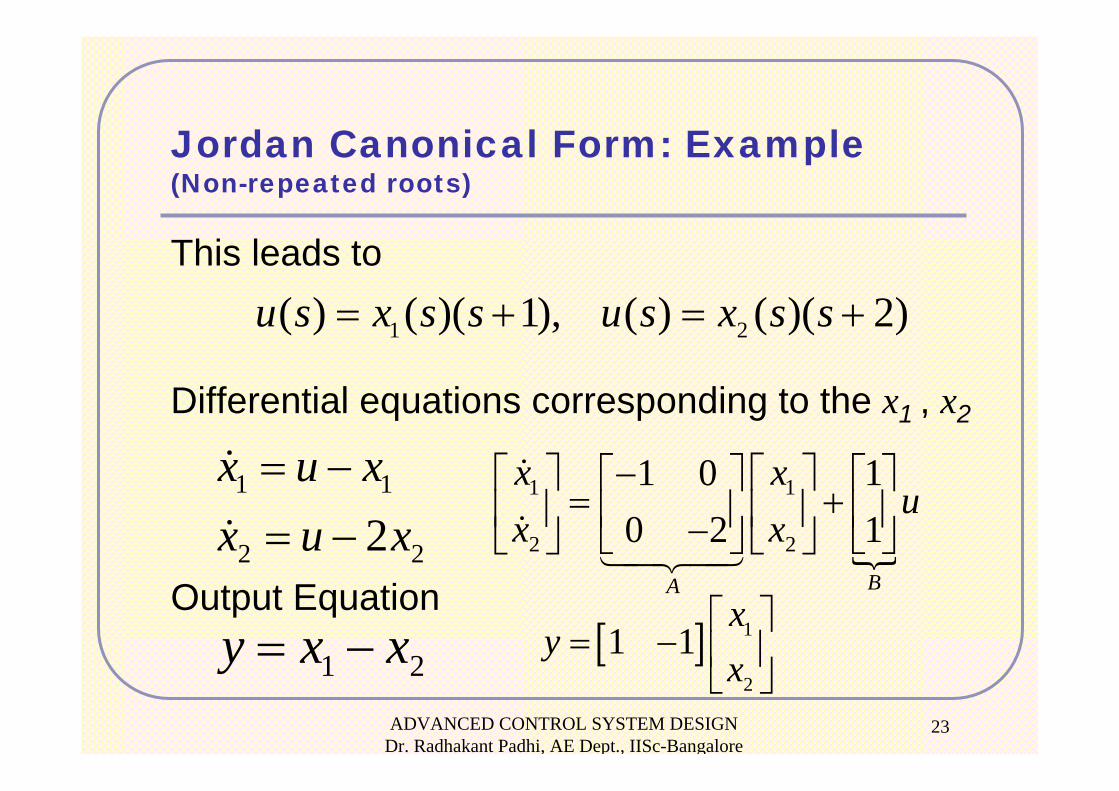
This leads to

Differential equations corresponding to the x1 , x2

Output Equation

1 1

2 22x u xx u x= −= −

21 xxy −=

1 2( ) ( )( 1), ( ) ( )( 2)u s x s s u s x s s= + = +

1 1

2 2

1 0 10 2 1

BA

x xu

x x−⎡ ⎤ ⎡ ⎤⎡ ⎤ ⎡ ⎤

= +⎢ ⎥ ⎢ ⎥⎢ ⎥ ⎢ ⎥−⎣ ⎦ ⎣ ⎦⎣ ⎦ ⎣ ⎦

[ ] 1

2

1 1x

yx⎡ ⎤

= − ⎢ ⎥⎣ ⎦


24

Jordan Canonical Form: ExampleRepeated Roots

( )3

21 1 1 2

32 2 2 3

3 3 3

Following the same procedure( ) 2( )( ) 3

Let( )( ) 3

3( )( ) 3

3( )( ) 3

3

y sH su s s

x sx s x x xsx sx s x x xsu sx s x x us

= =−

= ⇒ − =−

= ⇒ − =−

= ⇒ − =−


25

Jordan Canonical Form: ExampleRepeated Roots

Output Equation

Finally

( ) ( ) ( ) ( )

( ) ( ) ( )

3

3

( )

3 21

2 1 1 ( )( ) ( ) 23 3 33

( ) ( )12 2 2 ( )3 3 3

x s

u sy s u ss s ss

x s x s x ss s s

⎡ ⎤= = ⎢ ⎥

− − −− ⎢ ⎥⎣ ⎦

= = =− − −

[ ] [ ]

1 1

2 2

3 3

3 1 0 00 3 1 00 0 3 1

2 0 0 0X BX A

DC

x xx x ux x

y X u

⎡ ⎤ ⎡ ⎤ ⎡ ⎤ ⎡ ⎤⎢ ⎥ ⎢ ⎥ ⎢ ⎥ ⎢ ⎥= +⎢ ⎥ ⎢ ⎥ ⎢ ⎥ ⎢ ⎥⎢ ⎥ ⎢ ⎥ ⎢ ⎥ ⎢ ⎥⎣ ⎦ ⎣ ⎦ ⎣ ⎦ ⎣ ⎦

= +


26

Jordan Canonical Form:What if complex conjugate roots?

( ) ( )( )( )

1,2

2 2 2

Roots always exist in complex conjugate pairs!

2

2

j jHs j s j

s

s s

λ υ λ υσ ω σ ω

λ λσ ωυ

σ σ ω

+ −= +

+ − + +

+ −⎡ ⎤⎣ ⎦=+ + +

( )

( )

112 2

22

11,2

2

First companion form:0 1 0

2 1

2 2

xxu

xx

xy

x

σ ω σ

λσ ωυ λ

⎡ ⎤⎡ ⎤ ⎡ ⎤ ⎡ ⎤= +⎢ ⎥⎢ ⎥ ⎢ ⎥ ⎢ ⎥− + − ⎣ ⎦⎣ ⎦⎢ ⎥⎣ ⎦ ⎣ ⎦

⎡ ⎤= −⎡ ⎤ ⎢ ⎥⎣ ⎦

⎣ ⎦

The system can be realizedpartially in other forms (like First companion form)


27


28

lecture – 9 conversion between state space and … 10.pdflecture – 9 conversion between state...

Documents