lecture 9 - harvey mudd college experimental engineering lecture 9 inertial measurement feb. 19,...

E80 Experimental Engineering

Lecture 9 Inertial Measurement

Feb. 19, 2013

http://www.volker-doormann.org/physics.htm Christopher M. Clark


Where is the rocket?


Outline

§  Sensors q  People q  Accelerometers q  Gyroscopes

§  Representations §  State Prediction §  Example Systems §  Bounding with KF


Sensors

§  People http://en.wikipedia.org/wiki/File:Bigotolith.jpg


Sensors

§  Accelerometers

a = k x / m


Sensors

§  Accelerometers q  The accelerometers are typically MEMS based q  They are small cantilever beams (~100 µm)

Khir MH, Qu P, Qu H - Sensors (Basel) (2011)


Sensors

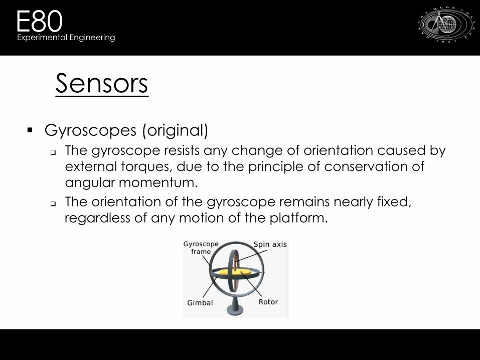
§  Gyroscopes (original) q  Mounted on two nested gimbals, the spinning wheel of the

gyroscope is free to take any orientation.

q  High spin rate leads to high angular momentum


Sensors

http://www.youtube.com/watch?v=cquvA_IpEsA


Sensors

§  Gyroscopes (original) q  The gyroscope resists any change of orientation caused by

external torques, due to the principle of conservation of angular momentum.

q  The orientation of the gyroscope remains nearly fixed, regardless of any motion of the platform.


Sensors

§  Gyroscopes (original) q  Gyroscope orientation can be obtained by measuring the

angles between adjacent gimbals.


11

Sensors

§  MEMS (Microelectromechanical Systems) Gyroscopes q  Two masses oscillate back and forth from the center of rotation

with velocity v. q  A rotation will cause a Coriolis force in this coordinate frame.


12

Sensors

§  MEMS Gyroscopes q  Their deflection y is measured, to establish a force

FCoriolis = ky q  The acceleration is obtained since the mass is known

-2m |Ω x v| = FCoriolis


13

Sensors

§  Inertial Measurement Units q  3 Accelerometers q  3 Gyroscopes q  3 Magnetometers(?)

www.barnardmicrosystems.com


14

Sensors

§  Inertial Measurement Units Y


Outline

§  Sensors §  Representations

q  Cartesian Coordinate Frames q  Transformations

§  State Prediction §  Example Systems §  Bounding with KF


Representations

§  Cartesian Coordinate Frames q  We can represent the

3D position of a vehicle with the vector

r =[ x y z ]


Representations

§  Euler Angles q  We can represent the 3D

orientation of a vehicle with the vector ϕ = [ α β γ ]

Roll - α Pitch - β Yaw - γ


Representations

§  Where do we place the origin? q  We can fix the origin at a

specific location on earth, e.g. a rocket’s launch pad.

q  This is called the global or inertial coordinate frame

X

Y

Z

r =[x y z]


Representations

§  Where do we place the origin? q  We can ALSO fix the origin on a

vehicle. q  This is called the local

coordinate frame

X

Y

Z

Z X

Y

r =[x y z]


Representations

§  Where do we place the origin? q  We must differentiate between

these two frames. q  What is the real difference

between these two frames? q  A Transformation consisting of a

rotation and translation

XG

YG

ZG

ZL XL

YL

r =[x y z]


Representations

§  Transformations q  The rotation can be

about 3 axes (i.e. the roll, pitch, yaw)

ZL

XL

YL

XG

YG

ZG

α

β

γ


Representations

§  Transformations q  The rotation can be

about 3 axes (i.e. the roll, pitch, yaw)

ZL XL

YL

XG

YG

ZG


Representations

§  Transformations q  The translation can

be in three directions

r =[x y z]

ZL XL

YL

XG

YG

ZG


Representations

§  Rotations q  In 2D, it is easy to

determine the effects of rotation on a vector

q2 = cos(α) -sin(α) q1 sin(α) cos(α)

= R(α) q1

Y

q1

X

α

q2


Representations

§  Rotations q  In 3D, we can use similar

rotation matrices

q2 = 1 0 0 q1 0 cos(α) -sin(α)

0 sin(α) cos(α)

= Rx(α) q1

q1 q2

XG

YG

ZG

α


Representations Rx(α) = 1 0 0 0 cos(α) -sin(α)

0 sin(α) cos(α) Ry(β) = cos(β) 0 sin(β) 0 1 0

-sin(β) 0 cos(β) Rz(γ) = cos(γ) -sin(γ) 0 sin(γ) cos(γ) 0 0 0 1


Representations

§  Rotations q  For 3 rotations, we can write a general Rotation Matrix

R(α, β, γ) = Rx(α) Rx(β) Rx(γ)

q  Hence, we can rotate any vector with the general Rotation Matrix

q2 = R(α, β, γ) q1


Outline

§  Sensors §  Representations §  State Prediction

q  Updating R(t) q  Updating r(t)

§  Example Systems §  Bounding Errors with KF


State Prediction

§  Strapdown Inertial Navigation q  Our IMU is fixed to the

local frame q  We care about the

state of the vehicle in the global frame

r =[x y z]

ZL XL

YL

XG

YG

ZG IMU


Updating R(t)

Given: ωL(t) = [ ωx,L(t) ωy,L(t) ωz,L(t) ]

Find: R(t)


Updating R(t) §  Lets define the rotational velocity matrix based on

our gyroscope measurements ωL= [ωx,L(t) ωy,L(t) ωz,L(t)]

Ω(t) = 0 -ωz(t) ωy(t) ωz(t) 0 -ωx(t) -ωy(t) ωx(t) 0


Updating R(t) §  It can be shown that the vehicle rotating with

velocity Ω(t) for δt seconds will (approximately) yield the resulting rotation Matrix R(t+δt):

R(t+δt) = R(t) [ I + Ω(t)δt ]


Updating r(t)

Given: aL = [ ax,L ay,L az,L ] R(t)

Find: rG = [ ax,L ay,L az,L ]


Updating r(t)


Updating r(t) §  First, convert to global reference frame

aG(t) = R(t) aL(t)

§  Second, remove gravity term aG(t) = [ ax,G(t) ay,G(t) az,G(t)-g ]


Updating r(t) §  Third, integrate to obtain velocity

vG(t) = vG(0) + aG(τ) dτ

§  Fourth, integrate to obtain position rG(t) = rG(0) + vG(τ) dτ

t 0

t 0


Updating r(t) §  Third, integrate to obtain (approximate) velocity

vG(t+δt) = vG(t) + aG(t+δt) δt

§  Fourth, integrate to obtain (approximate) position rG(t+δt) = rG(t) + vG(t+δt) δt


Outline

§  Sensors §  Representations §  State Prediction §  Example Systems

q  LN-3 q  The Jaguar

§  Bounding Errors with KF


39

Example Systems

§  LN-3 Inertial Navigation System q  Developed in 1960’s q  Used gyros to help steady the

platform q  Accelerometers on the platform

were used to obtain accelerations in global coordinate frame

q  Accelerations (double) integrated to obtain position


Example Systems

§  http://www.youtube.com/watch?feature=player_embedded&v=ePbr_4yMehs


Example Systems

§  The Jaguar Lite q  Equipped with an

IMU, camera, laser scanner, encoders, GPS


Example Systems

§  The Jaguar Lite q  GUI provides

acceleration measurements


Example Systems

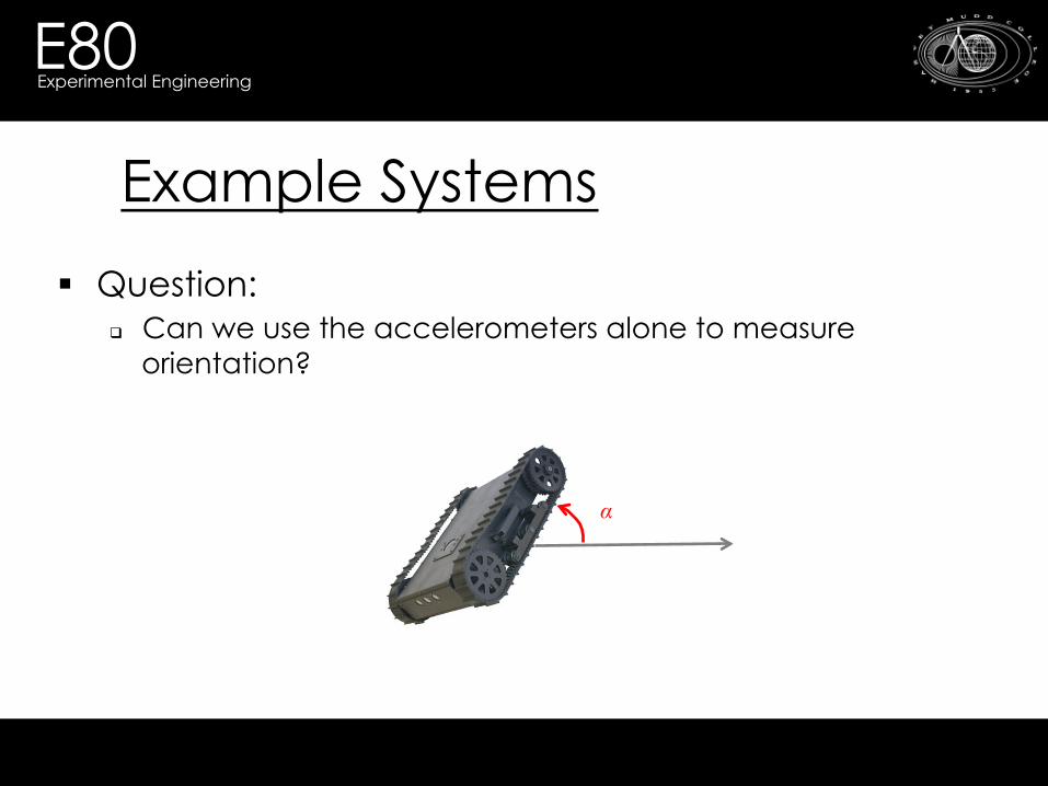
§  Question: q  Can we use the accelerometers alone to measure

orientation?

α


Outline

§  Sensors §  Representations §  State Prediction §  Example Systems §  Bounding Errors with KF

q  Exteroceptive Sensing q  Fusing measurements


Bounding our Errors

§  Exteroceptive sensors q  Drift in inertial navigation is a problem q  We often use exteroceptive sensors – which measure outside

the robot – to bound our errors q  Examples include vision systems, GPS, range finders


Bounding our Errors

§  Exteroceptive sensors q  We can fuse measurements, e.g. integrated accelerometer

measurements and range measurements, by averaging. q  For example, consider the 1D position estimate of the jaguar.

x = 0.5 ( xIMU + (xwall - xlaser) )

xIMU is the double integrated IMU measurement xwall is the distance from the origin to the wall xlaser is the central range measurement


Bounding our Errors

§  Exteroceptive sensors q  Lets weight the average, where weights reflect

measurement confidence

x = wIMU xIMU + wlaser(xwall - xlaser) wIMU + wlaser


Bounding our Errors

§  Exteroceptive sensors q  This leads us to a 1D Kalman Filter

xt = xIMU,t + Kt [(xwall – xlaser,t) - xIMU,t ]

Kt = σ2

IMU σ2

IMU + σ2laser

σ2x = (1 – Kt ) σ2

IMU


Bounding our Errors

§  IMU q  Higher sampling rate q  Small errors between time steps (maybe centimeters) q  Uncertainty increases q  Large build up over time (unbounded)

§  GPS q  Lower sampling rate q  Larger errors(maybe meters) q  Uncertainty decreases q  No build up (bounded)


Bounding our Errors

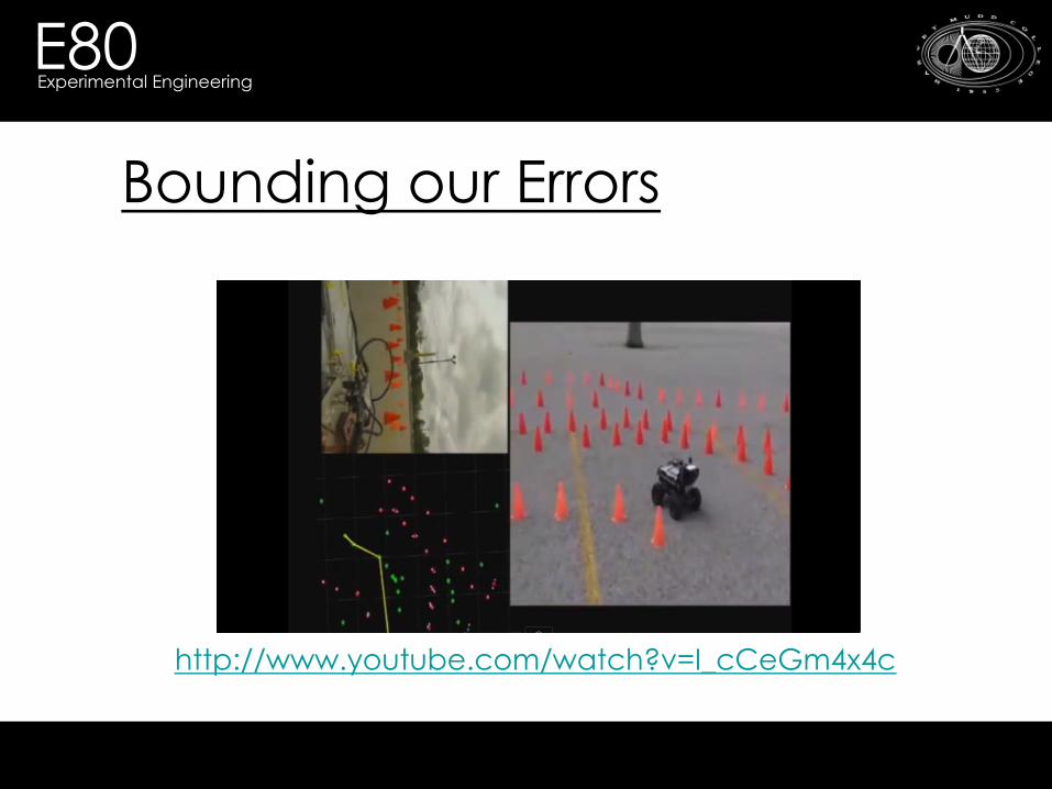
http://www.youtube.com/watch?v=I_cCeGm4x4c

lecture 9 - harvey mudd college experimental engineering lecture 9 inertial measurement feb. 19,...

Documents