Lecture 9: Leftovers, or random

issues with OLS

Functional form

misspecification

Proxy variables

Measurement error

Missing data

Nonrandom samples

Influential data

Least absolute deviation (LAD)

Scaling offending

Functional Form Misspecification

Functional form misspecification is a special type of

missing variable problem because the missing variable is

a function of nonmissing variables.

Examples: missing a squared term, an interaction, or

log(x).

As such, it is possible to fix functional form

misspecification if that’s your only problem.

RESET test can identify general functional form

problems but it can’t tell you how to fix them.

Functional Form Misspecification,

RESET test

The test is easy to implement. After your regression,

generate fitted values, and powers of fitted values,

usually just squared and cubed values.

Estimate the original equation, adding the squared and

cubed fitted values to the Xs:

Test the joint hypothesis that δ1 and δ2 are equal to zero

using either an LM or F test.

If you reject the null, you have functional form

misspecification.

2 3

0 1 1 1 2ˆ ˆ

k ky x x y y e

Functional Form Misspecification,

in practice

In practice, in criminology, the only functional form

misspecification that you might be asked about in a

journal article review is age. If the ages of your sample

span the curvy part of the age crime curve, you ought to

have a squared age term in there.

If functional form is misspecified, ALL of your parameter

estimates are biased.

Do in-class worksheet #1

Proxy variables

In the social science in particular, we often cannot

directly measure constructs that we are interested in. So

we often have to use proxy variables as a stand-in for

what we really want.

A good proxy:

Is strongly correlated with what we really want to

measure.

Renders the correlation between included variables

and the unobserved construct zero.

Proxy variables in criminology

For self-control:

11-item scale representing inclination to act impulsively (Mazzerolle

1998)

Enjoy making risky financial investments / taking chances with

money (Holtfreter, Reisig & Pratt 2008)

Gambling, smoking & drinking (Sourdin 2008)

For social support:

Marriage (Cullen 1998)

Ratio of tax deductible contributions to total number of returns

(Chamlin et al. 1999)

For social altruism:

United Way contributions (Chamlin & Cochran 1997)

For violent crime:

Homicide

Lagged dependent variables as

proxies

Because of continuity in individual offending and macro-

level crime rates, lagged dependent variables are very

powerful predictors of crime.

However, if your focal concern is the impact of some

other variable, say gang membership for example,

including a lagged dependent variable changes the

nature of your parameter estimate for gang membership.

It is now a question of whether gang membership leads

to a change in offending.

Furthermore, a lagged dependent variable can introduce

measurement error in an independent variable that is

correlated with measurement error in the dependent

variable.

Measurement error

Not all error is created equally. The consequences of random and nonrandom measurement error are very different.

Random measurement error: there is no correlation between the true score and the error with which it is measured independent variables: unbiased estimates, but inefficient

(standard errors go up, r-squared goes down)

dependent variables: estimates biased downward for bivariate

case, unknown bias for multivariate case

Measurement error

Non-random measurement error: the degree to which a particular xj is measured with error is related to values of xk, where k may be equal to j or not, and xk may or may not be observed.

Effects of non-random measurement error depend on the specific nature of the error. But typically results in biased estimates.

Systematic over- or under-estimation of an independent variable X or the dependent variable Y, will bias the intercept only, and is therefore less concerning.

Nonrandom samples / missing

data

Ideally, you possess a random sample of data from the population you are interested in studying, with no missing data. Usually, however, this is not the case.

If the nonrandomness is known, as is the case with stratified sampling, you can usually modify your regressions with sampling weights to obtain unbiased estimates.

Exogenous sample selection: known nonrandomness based on an independent variable. This is not a problem either, but it changes the meaning of your parameters. You can no longer make inferences to the population of interest, but to the population that corresponds to your nonrandom sample. Example: many variables in the NLSY97 are only asked of certain age

cohorts. Using these requires dropping a large percentage of the data, but doesn’t bias the estimates for the represented age cohort.

Nonrandom samples / missing

data

Endogenous sample selection: based on the dependent variable This biases your estimates.

Missing data can lead to nonrandom samples as well.

Most regression packages perform listwise deletion of all variables included in OLS. That means that if any one of the variables is missing, then that observation is dropped from the analysis.

If variables are missing at random, this is not a problem, but it can result in much smaller samples.

20 variables missing 2% of observations at random results in a sample size that is 67% of the original (.98^20)

Nonrandom samples / missing

data

Usually data is not missing at random.

Ex: missing self-reported drug use, property offending,

sexual behavior, etc.

When data is not missing at random, and you run

your models with listwise deletion, the resulting

parameter estimates are biased for the population of

interest.

Dealing with missing data

It is advisable to compare data for the observations dropped

from your sample and those retained.

Create a dummy variable for being in your final sample. (1=in sample,

0=not in final sample)

Demographic variables will typically be nonmissing for all

cases, so you can compare those using independent samples

t-tests.

If you can find no significant differences between the included

and excluded samples, you can make the case that data is

missing at random, and proceed as usual.

If you find many significant differences, you have a few

options.

Dealing with missing data, cont.

Describe the type of observations that make it into your regression analysis to indicate what population your parameters refer to. (weak)

Correct for sample selection bias using the Heckman Two-Step Correction (see Bushway, Johnson & Slocum 2007) – we’ll cover this next time (maybe)

Perform multiple imputation (mi command in Stata) Impute many datasets (~30)

Obtain estimates from each dataset

Recombine estimates

Influential Data

Is there an observation in your sample so

influential that removing it would

substantially change your regression

estimates?

If so, what does this mean and what should

be done?

Incorrect data? Fix it.

Observation drawn from different population.

Drop it.

Identifying Influential Data

Residuals by themselves are not informative. Both of the

circled points below are outliers, in different ways.

The first has a large residual, but has little leverage

(influence) over the regression line.

The second has a small residual, but a lot of leverage.

Identifying Influential Data, graphs

One way to check for influential data is to

run scatter plots.

In stata, you can call up a matrix of scatter

plots all at once: . graph matrix homrate poverty IQ het gradrate fem_hh, half

You can also identify particular

observations with labels: . scatter homrate poverty, mlabel(state)

Identifying Influential Data poverty

IQ

het

gradrate

fem_hh

homrate

5 10 15 20

95

100

105

95 100 105

0

.5

1

0 .5 1

50

100

50 100

8

10

12

14

8 10 12 14

0

5

10

15

Identifying Influential Data

New Hampshire

New Jersey

VermontMinnesota

HawaiiUtah

DelawareVirginia

ConnecticutNebraska

Maryland

Idaho

Alaska

MassachusettsWisconsinWashington

Wyoming

Nevada

Florida

North Dakota

Pennsylvania

Iowa

Colorado

IllinoisMissouri

South Dakota

Michigan

OregonRhode Island

OhioKansas

Maine

IndianaNorth Carolina

California

Montana

Arkansas

Georgia

New York

Kentucky

Tennessee

South Carolina

Arizona

West Virginia

OklahomaTexas

Alabama

New Mexico

Louisiana

Mississippi

05

10

15

ho

mra

te

5 10 15 20poverty

Identifying Influential Data, hat

values

Another way to identify influential data after

running a regression model is to look at “hat

values.”

Hat values are a measure of influence of each

data point. They range from 1/n to 1, their mean

is k/n where k is the number of regressors in the

model, including the intercept.

The more unusual the Xs for any observation, the

greater its influence on the regression model.

In stata use the “, hat” option for predict.

Identifying Influential Data,

studentized residuals

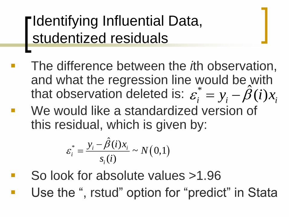
The difference between the ith observation, and what the regression line would be with that observation deleted is:

We would like a standardized version of this residual, which is given by:

So look for absolute values >1.96

Use the “, rstud” option for “predict” in Stata

* ˆ( )i i iy i x

*ˆ( )

~ 0,1( )

i ii

i

y i xN

s i

Identifying Influential Data, dfbetas

Studentized residuals give us a general

sense of which observations are most

influential.

Dfbetas tell us which observations most

impact specific parameters.

ˆ ( )

ˆ ˆ ( )

j

j j

ji

i

iDFBETAS

s

Identifying Influential Data, dfbetas

If the absolute value of dfbeta is greater

than 2/sqrt(N), then it’s considered

problematic.

In Stata you can create all the dfbeta

estimates at once:

. dfbeta

Identifying Influential Data, diagnostic

graphs

There are two kinds of graphs that are useful after a regression

Added-variable, or partial regression plots show the relationship between one independent variable and the dependent variable after adjusting for all other independent variables (“avplot x” or “avplots”)

Residual vs. leverage plots can show which observations have high residuals and high leverage, which can be the most problematic (lvr2plot)

Worksheet: #4-6

Dealing With Influential Data

So you have some influential data. What do you

do about it?

Look at it. Are there any data entry errors? If so,

fix them. If you can’t, throw it out.

Is this observation drawn from a different

distribution (e.g. DC vs states)? If so, consider

throwing it out.

Otherwise, keep it. But what if your key

independent variable is statistically significant if

and only if you keep a single observation?

Least Absolute Deviation, or quantile

regression

In some applications, it is preferable to model the expected median given x1 through xk, or the expected 25th or 75th percentile.

This is extremely uncommon in criminology.

I could find one application of this method in a top criminology journal:

“Modeling the distribution of sentence length decisions under a guidelines system: An application of quantile regression methods” by Chet Britt in JQC 2009

If interested, start there and work backwards.

“qreg” in Stata

• Should we combine measures of different

types of offending into a single scale?

•Behaviors considered “criminal” are so

disparate that illegality itself may seem like

their only shared characteristic.

•How can they be combined?

*This topic was originally presented at ASC 2009 and

then published in the Journal of Quantitative

Criminology in 2012.

The problem of scaling offending

“Is one homicide to be equated with 10 petty

offenses? 100? 1000? We may sense that

these are incommensurables and so feel that

the question of comparing their magnitude is a

nonsense question.”

- Robert Merton (1961, emphasis in original)

The Problem, cont.

Options for scaling offending

• Prevalence (0/1)

• Frequency

• weighted by seriousness

• Variety

• Summed ordinal scale

• Often transformed in some way: logged, z-score,

factor weighted, etc.

• Latent trait estimated from Rasch models (item response

theory)

• Other ad hoc method

• Limiting to one crime type or official data? See above.

History of Scaling Offending

• Guttman scaling

• an ordered variety scale, popular in the

1960s, used as late as 2003 (Tittle et al.)

to describe levels of self-control

• Sellin-Wolfgang seriousness scale

• 21 different offenses (141 originally)

scaled according to seriousness ratings in

survey research

• Ex: Homicide=26, serious assault=7, petty

theft=1

History of Scaling Offending, cont.

• “Measuring Delinquency” (Hindelang, Hirschi

& Weis 1981)

• Modest support for unidimensional scale

of offending

• Recommended “ever variety” scale:

number of types of offenses committed

• Higher reliability than frequency scores

• Higher correlation with official reports

than frequency scores

Item Response Theory

• latent trait, theta (θ), accounts for the

observed response patterns

• α reflects strength of relationship between a

single item’s responses and latent trait

• b reflects threshold for which question

response category (or more serious

category) is 50% likely

• After item-specific parameters estimated,

theta is estimated for each person

Scaling Offending Today

• Of 130 individual-level quantitative articles in

5 criminology journals in 2007-8

• 76 (58%) prevalence (0/1)

• 53 (41%) frequency

• 15 (12%) summed or transformed

category

• 12 (9%) variety

• 5 (4%) weighted frequency

• 5 (4%) IRT

Scaling example, data

National Longitudinal Survey of Youth

1997

• 8,984 youths 12-16 years old as of

12/31/1996

• Wave 3 used, when youth were, on average

17.4 years old (s.d.=1.4), N=8209

• 6 offending items: intentional destruction of

property, petty theft (<$50), serious theft

(>$50), attacking with intent to hurt, selling

drugs

Item-specific descriptives

Prevalence Frequency (s.d.)

Destruction of property

Theft <$50

Theft >$50

Other property crime

Attacking to hurt

Selling drugs

.0798

.0867

.0277

.0273

.0959

.0573

.37 (3.32)

.55 (4.08)

.17 (2.37)

.19 (2.47)

.37 (3.16)

1.18 (8.44)

Total .2444 2.83 (14.73)

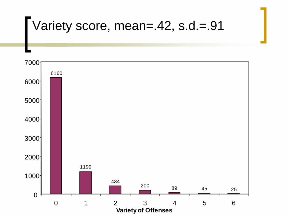
Variety score, mean=.42, s.d.=.91

6160

1199

434 200

89 45 25 0

1000

2000

3000

4000

5000

6000

7000

0 1 2 3 4 5 6 Variety of Offenses

Frequency

IRT Results

Item

Item

Discrimination

Response Location

a b1-2 b3-4 b5+

1: Destruction of property

2: Theft <$50

3: Theft >$50

4: Other property crime

5: Attacking to hurt

6: Selling drugs

2.53

2.12

3.01

3.33

1.62

1.96

1.74

1.86

2.19

2.20

2.00

2.14

2.34

2.50

2.60

2.54

2.85

2.34

2.59

2.72

2.76

2.71

3.28

2.45

d

Distribution of IRT criminality

estimates

6399

0 0 0

731 320 281 209 128 73 37 15 11 5

0

1000

2000

3000

4000

5000

6000

7000

0 0.5 1 1.5 2 2.5 3

latent criminality

Fre

qu

en

cy

Conclusions

Prevalence

Sometimes most appropriate scale (i.e. conviction,

imprisonment, homicide)

When multiple items are combined, most prevalent (least

serious) contributes the most variation

Easy to interpret as IV/DV

Linear probability / Logit / Probit models

Frequency

Multiple item scales are dominated by high frequency items

Typically very skewed

Easy to interpret as IV/DV

Negative binomial/poisson models

Weighting by seriousness makes results less interpretable

Conclusions, cont.

Variety*

Limits contribution of less serious items

Highly correlated with IRT estimates (.92)

Slightly more difficult to interpret results as IV/DV

Negative binomial/poisson models

HH&W were right!, reasonable approximation of criminality

Variety scales are similar to summed category scales in that

they impose only two categories before summing

As the number of categories increases in summed category

scales, the influence of less serious items on the scale

increases.

Conclusions, cont.

IRT

Explicitly models relationship between criminality and offending

questions

Reveals information about people, and about behaviors

Extra estimation step adds error to scale that requires extra

work to correct

Recent work estimates model in single step (Osgood & Schreck, 2007)

Complicated interpretations

Tobit models?, need wide breadth of items

Next time:

bye week for homework

Read: Wooldridge Chapter 17, look over Bushway et al.,

2007, Smith & Brame, 2003