lecture 9: sampling distributions
TRANSCRIPT

Lecture 9: Sampling Distributions
MSU-STT-351-Sum-19B
(P. Vellaisamy: MSU-STT-351-Sum-19B) Probability & Statistics for Engineers 1 / 29

Sampling Distributions
Statistics & Their Distributions
Let X = (X1, . . . ,Xn) be a random sample from F(x |θ), where θ is theunknown parameter. That is, each Xi has the cdf F(x |θ) and Xi ’s areindependent.
(i) A statistic T is any value that can be calculated from sample data, thatis, T = T(X1, . . . ,Xn) is a function of X1, . . . ,Xn. For example, X̄ and S2
are sample statistics.
(ii) A statistic T(X), when takes a real value, is also random variable. Foran observed X = x, T(x) denotes a numerical value.
(iii) The probability distribution of T(X) is called a sampling distribution.
(P. Vellaisamy: MSU-STT-351-Sum-19B) Probability & Statistics for Engineers 2 / 29

Sampling Distributions
Random Samples(i) The distribution of a statistic T calculated from a sample with anarbitrary joint distribution can be very difficult.
(ii) Often, we assume that our data is a random sample X1, . . . ,Xn from adistribution F(x |θ). This means that (a) The Xi ’s are independent. (b) Allthe Xi ’s have the same probability distribution.
Example 1 (Ex 37): A particular brand of dishwasher soap is solid in threesizes; 25oz, 40oz, and 65oz. Twenty percent of all purchasers select a25oz box, 50% select a 40oz box, and the remaining 30% choose a 65ozbox. Let X1 and X2 denote the package sizes selected by twoindependently selected purchasers.
(a) Find the sampling distribution of X , E(X), and compare it with µ.(b) Determine the sampling distribution of the sample variance S2,
calculate E(S2) and compare to σ2.
(P. Vellaisamy: MSU-STT-351-Sum-19B) Probability & Statistics for Engineers 3 / 29

Sampling Distributions
Solution: Note both X1,X2 ∈ {25, 40, 65} and have the same distributionas that of the rv X with
P(X = 25) = .2, P(X = 40) = .5, P(X = 65) = .3
which has the mean µ = 44.5 and the variance σ2 = 212.25.
Since X1 and X2 are independent, their joint distribution can be found andit is given below. NoteP(X1 = 25; X2 = 25) = P(X1 = 25)P(X2 = 25) = 0.2 × 0.2 = 0.04.
p(x1) 0.20 0.50 0.30p(x2) X2|X1 25 40 650.20 25 0.04 0.10 0.060.50 40 0.10 0.25 0.150.30 65 0.06 0.15 0.09
(P. Vellaisamy: MSU-STT-351-Sum-19B) Probability & Statistics for Engineers 4 / 29

Sampling Distributions
(a) Also, X = X1+X22 . The distribution of X is given below:
x 25 32.5 40 45 52.5 65p(x) 0.04 0.20 0.25 0.12 0.30 0.09
The mean of the above distribution is
E(X) = (25)(.04) + (32.5)(.20) + . . . + (65)(.09) = 44.5 = µ.
(b) Similarly, the distribution of S2 based on X1 and X2 is is
s2 0 112.5 312.5 800p(s2) 0.38 0.20 0.30 0.12
The mean of the distribution of S2 is
E(S2) = 212.25 = σ2.
(P. Vellaisamy: MSU-STT-351-Sum-19B) Probability & Statistics for Engineers 5 / 29

Sampling Distributions
Example 2 (Ex 40): A box contains ten sealed envelopes numbered1, . . . , 10. The first five contain no money, the next three each contains $5,and there is a $10 bill in each of the last two. A sample of size 3 isselected with replacement and you get the largest amount of theenvelopes selected.
If X1,X2 and X3 denote the amounts in the selected envelopes, the statisticof interest is M = the maximum of X1,X2 and X3.
(a) Obtain the probability distribution of this statistic.
(b) Describe how you would carry out a simulation experiment to comparethe distributions of M for various sample sizes. How would you guess thedistribution would change as n increases?
(P. Vellaisamy: MSU-STT-351-Sum-19B) Probability & Statistics for Engineers 6 / 29

Sampling Distributions
Solution:(a) Possible values of M are: 0, 5, 10. Note M = 0 when all 3 envelopescontain 0 money, hence P(M = 0) = (0.5)3 = 0.125. Also, M = 10 whenthere is at least one envelope with $10. Hence,P(M = 10) = 1 − P(no envelopes with $10) = 1 − (0.8)3 = 0.488.Finally, P(M = 5) = 1 − [0.125 + 0.488] = 0.387.
Thus, we obtain the sampling distribution of M as
m 0 5 10p(m) 0.125 0.387 0.488
An alternative solution would be to list all 27 possible combinations using atree diagram and computing probabilities directly from the tree.
(P. Vellaisamy: MSU-STT-351-Sum-19B) Probability & Statistics for Engineers 7 / 29

Sampling Distributions
(b) Let X denote the amount contained in a randomly selected envelope.Its population distribution (also called population distribution) is as follows:
x 0 5 10p(x) 1/2 3/10 1/5
Write a computer program to generate the digits 0-9 from a uniformdistribution. Assign a value of 0 to the digits 0-4, a value of 5 to digits 5-7,and a value of 10 to digits 8 and 9. Generate samples of increasing sizes,keeping the number of replications constant and compute M from eachsample.
As n, the sample size, increases, P(M = 0) goes to zero, P(M = 10) goesto one. Furthermore, P(M = 5) goes to zero, but at a slower rate thanP(M = 0).
(P. Vellaisamy: MSU-STT-351-Sum-19B) Probability & Statistics for Engineers 8 / 29

Sampling Distributions
Deriving a Sampling Distribution
Example 3: An automobile service charges $40, $45 and $50 for atune-up of four-, six- and eight-cylinder cars. The revenue (say X )distribution of cars is
x 40 45 50p(x) 0.2 0.3 0.5
which has µ = 46.5 and σ2 = 15.25.
Only two jobs are done in a day. Let Xi =revenue from i-th service,i = 1, 2. The distribution of X1,X2 is given below:
(P. Vellaisamy: MSU-STT-351-Sum-19B) Probability & Statistics for Engineers 9 / 29
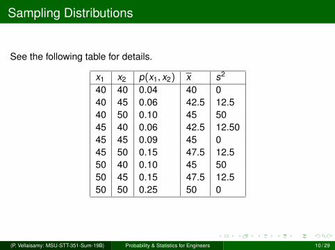
Sampling Distributions
See the following table for details.
x1 x2 p(x1, x2) x s2
40 40 0.04 40 040 45 0.06 42.5 12.540 50 0.10 45 5045 40 0.06 42.5 12.5045 45 0.09 45 045 50 0.15 47.5 12.550 40 0.10 45 5050 45 0.15 47.5 12.550 50 0.25 50 0
(P. Vellaisamy: MSU-STT-351-Sum-19B) Probability & Statistics for Engineers 10 / 29

Sampling Distributions
The sampling distribution of x is
x 40 42.5 45 47.5 50p(x) 0.04 0.12 0.29 0.30 0.25
Note P(X = 42.5) = p(42.5) = 0.06 + 0.06, using the table in theprevious page.
Similarly, the sampling distribution of S2 is
s2 0 12.5 0PS2(s2) 0.38 0.42 0.20
(P. Vellaisamy: MSU-STT-351-Sum-19B) Probability & Statistics for Engineers 11 / 29

Sampling Distributions
Data from Continuous Distributions
Example 4 (5.21)
Let X1 and X2 denote a random sample (service times) of size 2 fromexponential distribution with parameter λ (or G(1, 1/λ)). Then
X1 + X2 ∼ G(2, 1/λ).
Then the sample mean X = X1+X22 ∼ G(2, 1/2λ) with density
f(x) =
{4λ2xe−2λx , if x > 00, otherwise.
(P. Vellaisamy: MSU-STT-351-Sum-19B) Probability & Statistics for Engineers 12 / 29

Sampling Distributions
Properties of Sample mean and Sample sum(i) Let X1, . . . ,Xn be a random sample from a distribution with mean valueµ and standard deviation σ. Then
E[x] = µx = µ;
V(x) = σ2x = σ2/n;
σx = σ/√
n.
(ii) Let Tn = X1 + X2 + . . . + Xn be the sample total. Then
E[Tn] = nµ;
V(Tn) = nσ2;
σTn =√
nσ.
(iii) If the original distribution of the Xi ’s is normal, then the distribution of Xand Tn are also normal.(P. Vellaisamy: MSU-STT-351-Sum-19B) Probability & Statistics for Engineers 13 / 29
Sampling Distributions
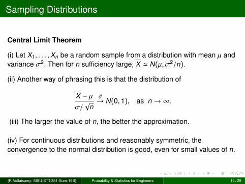
Central Limit Theorem
(i) Let X1, . . . ,Xn be a random sample from a distribution with mean µ andvariance σ2. Then for n sufficiency large, X ' N(µ, σ2/n).
(ii) Another way of phrasing this is that the distribution of
X − µ
σ/√
n
d→ N(0, 1), as n → ∞.
(iii) The larger the value of n, the better the approximation.
(iv) For continuous distributions and reasonably symmetric, theconvergence to the normal distribution is good, even for small values of n.
(P. Vellaisamy: MSU-STT-351-Sum-19B) Probability & Statistics for Engineers 14 / 29

Sampling Distributions
Convergence of means from U[−1, 1] to a normal shape
(i) The uniform distribution on the interval [−1, 1] has a mean of 0 and avariance of 1/3.
(ii) We simulate 50000 replications from the original distribution, mns01,from the distribution of the means of samples of sizes 2, 3, 4, 5, and 6.
(iii) Histograms of the means of the samples will show convergence to anormal shape and decreasing variance.
(iv) If we multiply the means of samples of size n by√
n we can put themall on the same scale to see the convergence to a normal shape.
(P. Vellaisamy: MSU-STT-351-Sum-19B) Probability & Statistics for Engineers 15 / 29

Sampling Distributions
Histograms of raw means of samples from U[-1,1].
(P. Vellaisamy: MSU-STT-351-Sum-19B) Probability & Statistics for Engineers 16 / 29

Sampling Distributions
Example 5 (Ex 47):
The inside diameter of a randomly selected piston ring is a normalrandom variable with mean value 12 cm and standard deviation .04cm.
(a) Calculate P(11.99 ≤ X ≤ 12.01) when n = 16.
(b) How likely is it that the sample mean diameter exceeds 12.01 whenn = 25?
(P. Vellaisamy: MSU-STT-351-Sum-19B) Probability & Statistics for Engineers 17 / 29

Sampling Distributions
Solution Given µ = 12cm σ = 0.04cm.(a) For n = 16, we have
P(11.99 ≤ X ≤ 12.01) = P(11.99 − 12
0.01≤ Z ≤
12.01 − 120.01
)= P(−1 ≤ Z ≤ 1)
= Φ(1) − Φ(−1)
= 0.8413 − 0.1587.
= 0.6826
(b) For n = 25, we haveP(X > 12.01) = P
(Z >
12.01 − 12.04/5
)= P(Z > 1.25)
= 1 − Φ(1.25)
= 1 − 0.8944
= .1056.
(P. Vellaisamy: MSU-STT-351-Sum-19B) Probability & Statistics for Engineers 18 / 29

Sampling Distributions
Example 6 (Ex 54):
Suppose the sediment density (g/cm) of a randomly selected specimenfrom a certain region is normally distributed with mean 2.65 and standarddeviation .85.
(a) If a random sample of 25 specimens is selected, what is the probabilitythat the sample average sediment density is at most 3.00? Between 2.65and 3.00?
(b) How large a sample size would be required to ensure that the firstprobability in part (a) is at least .99?
(P. Vellaisamy: MSU-STT-351-Sum-19B) Probability & Statistics for Engineers 19 / 29

Sampling Distributions
Solution. It is given that
µX = µ = 2.65, σx =σx√
n=.855
= 0.17
Hence,P(X ≤ 3.00) = P
(Z ≤ 3.00−2.65
.17
)= P(Z ≤ 2.65) = .9803
P(2.65 ≤ X ≤ 3.00) = P(X ≤ 3.00) − P(X ≤ 2.65) = .4803
(b) Since,
P(X ≤ 3.00) = P(Z ≤
3.00 − 2.65
0.85/√
n
)= 0.99
we have0.35
85/√
n= 2.33, from which n = 32.02.
Thus, n = 33 will suffice.
(P. Vellaisamy: MSU-STT-351-Sum-19B) Probability & Statistics for Engineers 20 / 29

Sampling Distributions
Linear Combinations and their means(i) For n random variables X1, . . . ,Xn and n constants a1, . . . , an, therandom variable
Y = a1X1 + a2X2 + . . . + anXn
is called a linear combination of the Xi ’s.(ii) Whether or not the Xi ’s are independent,
E[a1X1 + . . . + anXn] = a1E[X1] + . . . + anE[Xn].
Variances of linear combinations(i) If X1, . . . ,Xn are independent with variances σ2
1, . . . , σ2n, then
V(a1X1 + . . . + anXn) = a21V(X1) + . . . + a2
nV(Xn) = a21σ
21 + . . . + a2
nσ2n.
(ii) In general,V(a1X1 + . . . anXn) =
∑ni=1
∑nj=1 aiajCov(Xi ,Xj), where Cov(Xi ,Xj)
denotes the covariance between Xi and Xj .
(P. Vellaisamy: MSU-STT-351-Sum-19B) Probability & Statistics for Engineers 21 / 29

Sampling Distributions
The difference between random variables
(i) Note, Y = X1 − X2 is a special linear combination with a1 = 1, a2 = −1,and
E(X1 − X2) = E(X1) − E(X2);
(ii) When X1 and X2 are independent,
Var(X1 − X2) = a21Var(X1) + a2
2Var(X2)
= 12Var(X1) + (−1)2Var(X2)
= Var(X1) + Var(X2).
That is, the variance of the difference is the sum of the variances.
(P. Vellaisamy: MSU-STT-351-Sum-19B) Probability & Statistics for Engineers 22 / 29

Sampling Distributions
(ii) Remember that “Variances add” in the sense that even when you takethe difference of independent random variables, their variances add.But the standard deviations do not add:
σY =√σ2
1 + σ22 , σ1 + σ2.
The Case of Normal Random Variables
If X1, . . . ,Xn are independent normal N(µi , σi) variables, then
n∑i=1
aiXi ∼ N( n∑
i=1
aiµi ,
n∑i=1
a2i σ
2i
).
(P. Vellaisamy: MSU-STT-351-Sum-19B) Probability & Statistics for Engineers 23 / 29

Sampling Distributions
Example 7 (Ex 60): Five automobiles of the same type are to be driven ona 300-mile trip. The first two will use an economy brand of gasoline, andthe other three will use a name brand. Let X1,X2,X3,X4 and X5 be theobserved fuel efficiencies (mpg) for the five cars. Suppose these variablesare independent and normally distributed withµ1 = µ2 = 20, µ1 = µ2 = µ3 = 21 and σ2 = 5 for the economy brand and3.5 for the name brand. Define on rv Y by
Y =X1 + X2
2−
X3 + X4 + X5
3.
So, Y is a measure of the difference in efficiency between economy gasand name-brand gas. Compute P(Y ≥ 0) and P(−1 ≤ Y ≤ 1).
(P. Vellaisamy: MSU-STT-351-Sum-19B) Probability & Statistics for Engineers 24 / 29

Sampling Distributions
Solution. Note
µY =12
(µ1 + µ2) −13
(µ3 + µ4 + µ5) = −1;
σ2Y =
14σ2
1 +14σ2
2 +19σ2
3 +19σ2
4 +19σ2
5 = 3.167;
σY = 1.7795.
Thus,
P(Y ≥ 0) = P(Z ≥
0 − (−1)
1.7795
)= P(Z ≥ 0.56)
= 0.2877.
P(−1 ≤ Y ≤ 1) = P(0 ≤ Z ≤2
1.7795)
= P(0 ≤ Z ≤ 1.12)
= 0.3686.
(P. Vellaisamy: MSU-STT-351-Sum-19B) Probability & Statistics for Engineers 25 / 29

Sampling Distributions
Example 8 (Ex 64): Suppose your waiting time for a bus in the morning isuniformly distributed on [0, 8], whereas waiting time in the evening isuniformly distributed on [0, 10] independent of morning waiting time.(a) If you take the bus each morning and evening for a week, what is yourtotal expected waiting time?(b) What is the variance of your total waiting time?(c) What are the expected value and variance of the difference betweenmorning and evening waiting times on a given day?(d) What are the expected value and variance of the difference betweentotal morning waiting time and total evening waiting time for a particularweek?
(P. Vellaisamy: MSU-STT-351-Sum-19B) Probability & Statistics for Engineers 26 / 29

Sampling Distributions
SolutionLet X1, . . . ,X5 denote morning times and X6, . . . ,X10 denote eveningtimes. Then (a)
E(X1 + . . . + X10) = E(X1) + . . . + E(X10)
= 5E(X1) + 5E(X6)
= 5(4) + 5(5) = 45
(b)
Var(X1 + . . . + X10) = Var(X1) + . . . + Var(X10)
= 5Var(X1) + 5Var(X6)
= 5[6412
+10012
]=
82012
= 68.33
(P. Vellaisamy: MSU-STT-351-Sum-19B) Probability & Statistics for Engineers 27 / 29

Sampling Distributions
(c) E(X1 − X6) = E(X1) − E(X6) = 4 − 5 = −1.
Var(X1 − X6) = Var(X1) + Var(X6) = 6412 + 100
12 = 16412 = 13.67.
(d) E[(X1 + . . . + X5) − (X6 + . . . + X10)] = 5(4) − 5(5) = −5.
Var[(X1 + . . . + X5) − (X6 + . . . + X10)
]= Var(X1 + . . . + X5)
+Var(X6 + . . . + X10)
= Var(X1) + . . . + Var(X10)
= 68.33.
(P. Vellaisamy: MSU-STT-351-Sum-19B) Probability & Statistics for Engineers 28 / 29

Sampling Distributions
Home Work:Sect: 5.3 : 39, 42Sect: 5.4 : 46, 51, 55Sect: 5.5 : 59, 65, 71, 73
(P. Vellaisamy: MSU-STT-351-Sum-19B) Probability & Statistics for Engineers 29 / 29