lecture 9 two-sample test - isyeyxie77/isye2028/lecture9.pdf10-5 inference on the variances of two...

Lecture 9 Two-Sample Test

Fall 2013 Prof. Yao Xie, [email protected]

H. Milton Stewart School of Industrial Systems & Engineering Georgia Tech

Computer exam 1Histogram

Freq

uency

0

5

9

14

18

Bin

75 83.33333333 91.66666667 More

mean 89.90std 6.02 median 90

Midterm 2• Cover • Confidence interval

– One sided and two sided confidence intervals • Hypothesis testing

– Two approaches • Fixed significance level • p-‐value !

• Can bring a 1-‐page 1-‐sided cheat sheet !

• Make-‐up lecture on Friday Nov. 8: tentatively noon-‐1:20pm in the area in front of my office, Groseclose #339

Outline

• Test difference in the mean – Known variance – Unknown variance

• Test difference in sample proportion • Test difference in variance

Motivating Example• Safety of drinking water (Arizona Republic, May 27, 2001)

• Water sampled from 10 communities in Pheonix • And 10 communities from rural Arizona • Arsenic concentration (AC): determines water quality, ranges from 3 ppb to 48 ppb

• Is there a difference in AC between these two areas? If the difference is large enough?

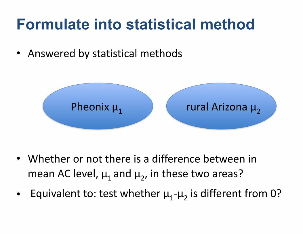
Formulate into statistical method

• Answered by statistical methods !!!!!

• Whether or not there is a difference between in mean AC level, μ1 and μ2, in these two areas?

• Equivalent to: test whether μ1-‐μ2 is different from 0?

Pheonix μ1 rural Arizona μ2

In general: comparing two populations

• Comparing two population means is often the way used to prove one population is different or better than another

• Competing Companies / Products

• Treatment vs. No Treatment

• New method vs. Old method

Test difference in the mean

Test difference in mean, variance known• Solve the following hypothesis test !!!!

• Assumptions for two sample inference

H0 :µ1 − µ2 = ΔH1 :µ1 − µ2 ≠ Δ

Test statistics

• A reasonable estimator for μ1 -‐ μ2 is

!!

• Under H0, its mean is Δ

• Its variance is !!

• Detection statistic

X1 − X2

σ 12

n1+σ 22

n2

Z = X1 − X2 − Δσ 12

n1+σ 22

n2

Detection for two sample difference

• For given significance level: • Reject H0 when

!!!!!

• And decide threshold b for that given significance level

Z > b

Z = X1 − X2 − Δσ 12

n1+σ 22

n2

p-value

• Probability of observing sample difference even more extreme, under H0

P Z > z0( )= 1−Φ z0( )

Example: paint drying time

Solution• test difference in mean drying time !!

• Δ ＝ 0

!!• form test statistic

H0 :µ1 − µ2 = ΔH1 :µ1 − µ2 > Δ

H0 :µ1 = µ2H1 :µ1 > µ2

Z = X1 − X2σ 12

n1+σ 22

n2

Fixed significance level approach• Reject H0 when

!!• Calculate:

Z = X1 − X2σ 12

n1+σ 22

n2

> zα

x1 − x2σ 12

n1+σ 22

n2

z0.05 = 1.65

>1.65Reject H0

α = 0.05

!

• Compute p-‐value: !!!!!

!!• p-‐value: !

• Reject H0 since its value is less than 0.01P Z > z0( )= 1−Φ z0( )= 1−Φ 2.52( )= 0.0059

Calculate p-value

Value of the statistic from data

Outline



Case 2: test difference in mean, variance unknown, true variance equal

• Solve the following hypothesis test !

!!• Variances are equal but unknown, so we “pool” the samples to estimate the variance !!!

• S1 and S2 are sample variances

H0 :µ1 − µ2 = ΔH1 :µ1 − µ2 ≠ Δ

Sp2 =(n1 −1)S1

2 + (n2 −1)S22

n1 + n2 − 2

Sp2 (n1 + n2 − 2)

σ 2 ~ χn1+n2−2

!19

X1 − X2 − ΔSp 1/ n1 +1/ n2

~ tn1+n2− 2

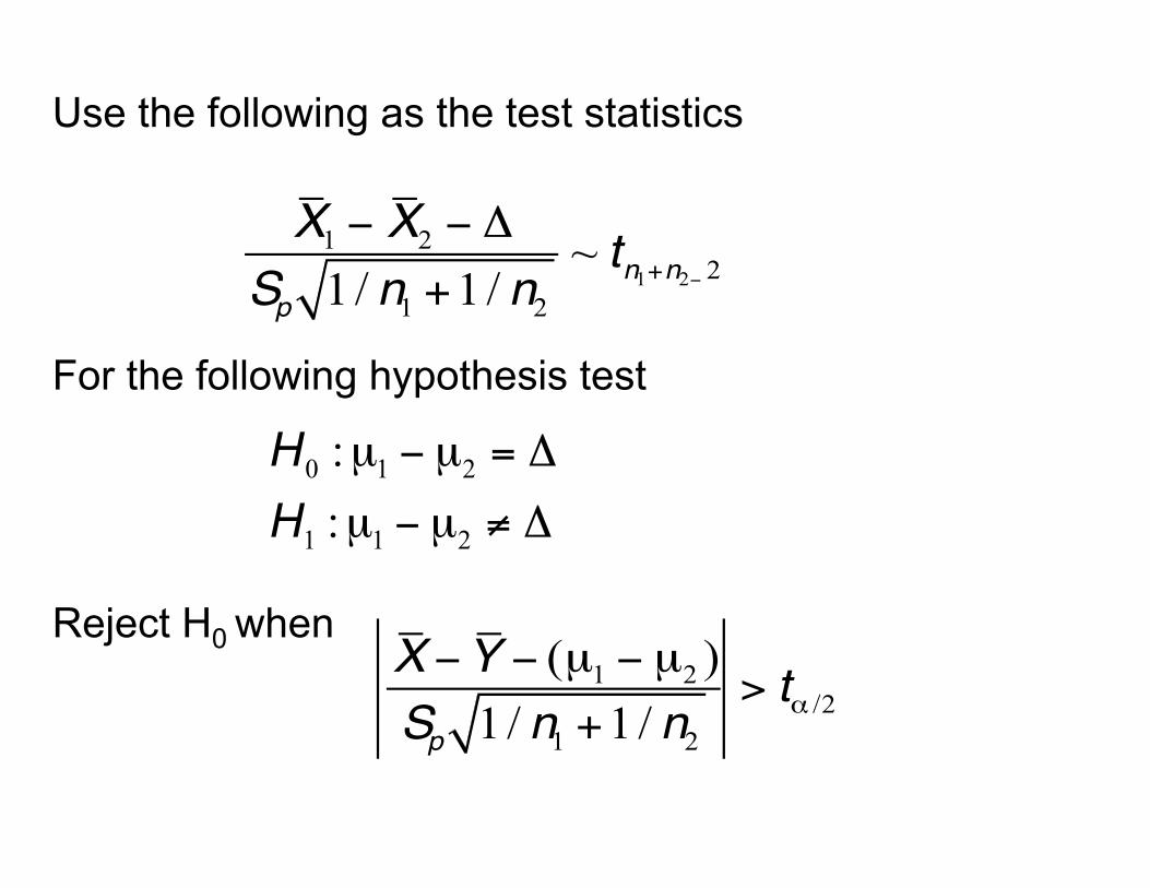
Use the following as the test statistics

H0 :µ1 − µ2 = ΔH1 :µ1 − µ2 ≠ Δ

For the following hypothesis test !!!!Reject H0 when

X −Y − (µ1 − µ2 )Sp 1/ n1 +1/ n2

> tα /2

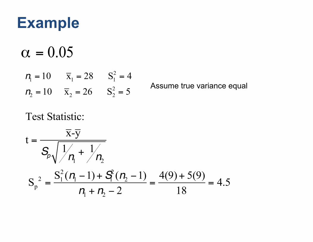
Example

n1 = 10 x1 = 28 S12 = 4

n2 = 10 x2 = 26 S22 = 5

Test Statistic:

t =x-y

Sp 1n1+ 1

n2

Sp2 =

S12 (n1 −1)+S1

2 (n2 −1)n1 + n2 − 2

=4(9)+ 5(9)

18= 4.5

Assume true variance equal

α = 0.05

Sp2 = 4.5

Recall degrees of freedom here is n + m – 2 = 18

t18,0.025 = 2.101

t = 28-264.5 1 /10 +1/10

= 2.11>2.101

p− value = P(|T| > 2.11)=2P(T > 2.11) = 2 × 0.0491=0.0982

Threshold:

Weakly reject H0

Calculate p-value

Outline



Formulation

• Two binomial parameters of interests • Two independent random samples are taken from 2 populations

• Estimation of sample proportion

X ~ Bin(n1, p1), Y ~ Bin(n2, p2) ⇒ p̂1 =Xn1, p̂2 =

Yn2

H0 : p1 = p2H1 : p1 ≠ p2

Test statistics

Z = p̂1 − p̂2p1 1− p1( )

n1+p2 1− p2( )

n2!!Pooled estimate !!Estimate the test statistic: p̂1 − p̂2

p̂ 1− p̂( ) 1n1+1n2

"

#$%

&'

p̂ = X1 + X2n1 + n2

Two-sided test

Z =p̂1 − p̂2 − p1 − p2( )p1 1− p1( )

n1+p2 1− p2( )

n2!For two-sided test, !!reject H0 when

H0 : p1 = p2H1 : p1 ≠ p2

p̂1 − p̂2

p̂ 1− p̂( ) 1n1+1n2

"

#$%

&'

> zα /2

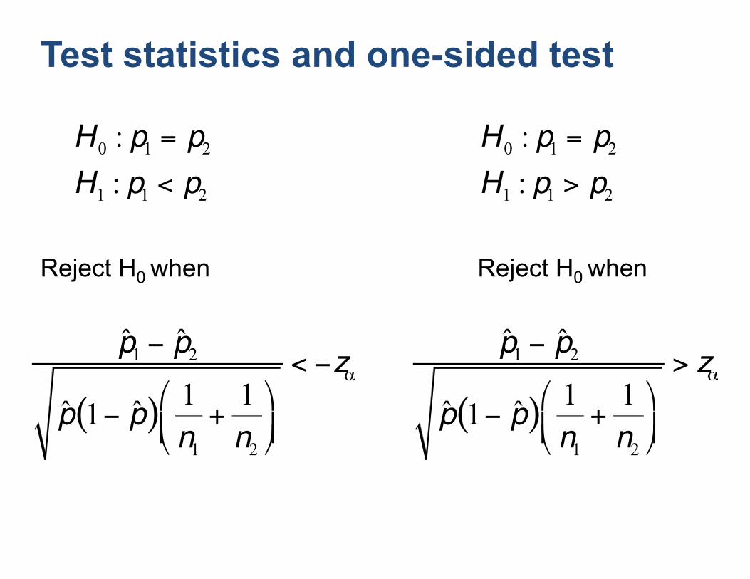
Test statistics and one-sided test

!Reject H0 when

p̂1 − p̂2

p̂ 1− p̂( ) 1n1+1n2

"

#$%

&'

< −zα

H0 : p1 = p2H1 : p1 < p2

!Reject H0 when

p̂1 − p̂2

p̂ 1− p̂( ) 1n1+1n2

"

#$%

&'

> zα

H0 : p1 = p2H1 : p1 > p2

Comparing 2 population proportions: Example

Standard drug X ~ Bin(100, p1)

New drug Y ~ Bin(100, p2)

A new drug is being compared to a standard using 200 clinical trials (100 patients for each group). For the new drug, 83 of 100 patients improved. For the standard, 72 of 100 improved. Is the new drug statistically superior?

X1 = 72,X2 = 83n1 = n2 = 100p̂1 = 0.72, p̂2 = 0.83z0.05 = 1.65

p̂1 − p̂2

p̂ 1− p̂( ) 1n1+1n2

"

#$%

&'

= −1.7323 < −1.65

H0 : p1 = p2H1 : p1 < p2

Reject H0

Fixed significance level approach

p-‐value !!!Less than α = 0.05, reject H0

P(Z < −1.7323) = 0.0418

p-value

Reject H0, with p-‐value 0.0418

Outline



Test difference in variance• two independent normal populations • means and variances of the two normals are unknown

• test whether or not two variances are the same

�31

10-5.1 F Distribution

Suppose that two independent normal populations are of interest, where the population meansand variances, say, !1, "2

1, !2, and "22, are unknown. We wish to test hypotheses about the

equality of the two variances, say, H0: "21 # "2

2. Assume that two random samples of size n1from population 1 and of size n2 from population 2 are available, and let S 2

1 and S 22 be the sam-

ple variances. We wish to test the hypotheses

(10-26)

The development of a test procedure for these hypotheses requires a new probabilitydistribution, the F distribution. The random variable F is defined to be the ratio of twoindependent chi-square random variables, each divided by its number of degrees of free-dom. That is,

(10-27)

where W and Y are independent chi-square random variables with u and v degrees of freedom,respectively. We now formally state the sampling distribution of F.

F #W$uY$v

H1: "21 % "2

2

H0: "21 # "2

2

10-5 INFERENCE ON THE VARIANCES OF TWO NORMAL DISTRIBUTIONS 383

Let W and Y be independent chi-square random variables with u and v degrees offreedom, respectively. Then the ratio

(10-28)

has the probability density function

(10-29)

and is said to follow the F distribution with u degrees of freedom in the numeratorand v degrees of freedom in the denominator. It is usually abbreviated as Fu,v.

f 1x2 #

& au ' v2 b auvbu$2 x 1u$22(1

& au2b & av2b c auvb x ' 1 d 1u'v2$2, 0 ) x ) *

F #W$uY$v

F Distribution

The mean and variance of the F distribution are ! # v!(v ( 2) for v + 2, and

Two F distributions are shown in Fig. 10-4. The F random variable is nonnegative, and thedistribution is skewed to the right. The F distribution looks very similar to the chi-square dis-tribution; however, the two parameters u and v provide extra flexibility regarding shape.

"2 #2v21u ' v ( 22u1v ( 2221v ( 42 , v + 4

JWCL232_c10_351-400.qxd 1/15/10 2:14 PM Page 383

Test based on sample variance ratio• Test statistics: ratio of two sample variances !!

• Need to introduce F distribution

�32

F = S12

S22








(10-26)


(10-27)


F #W$uY$v

H1: "21 % "2

2

H0: "21 # "2

2



(10-28)


(10-29)


f 1x2 #

& au ' v2 b auvbu$2 x 1u$22(1


F #W$uY$v

F Distribution



"2 #2v21u ' v ( 22u1v ( 2221v ( 42 , v + 4

JWCL232_c10_351-400.qxd 1/15/10 2:14 PM Page 383








(10-26)


(10-27)


F #W$uY$v

H1: "21 % "2

2

H0: "21 # "2

2



(10-28)


(10-29)


f 1x2 #

& au ' v2 b auvbu$2 x 1u$22(1


F #W$uY$v

F Distribution



"2 #2v21u ' v ( 22u1v ( 2221v ( 42 , v + 4

JWCL232_c10_351-400.qxd 1/15/10 2:14 PM Page 383

F distribution• A continuous distribution !!!!!

• mean = !

• we should reject H0 when

the statistic is large

Sample distribution

• Under H0 the detection statistic

�34

F = S12

S22 =

(n1 −1)S12 /σ 1

2⎡⎣ ⎤⎦ / (n1 −1)(n2 −1)S2

2 /σ 22⎡⎣ ⎤⎦ / (n2 −1)

σ 12 =σ 2

2( )

χn1−12

χn2−12

• has distribution


Let X11, X12, p , X1n1be a random sample from a normal population with mean !1 and

variance "21, and let X21, X22, p , X2n2

be a random sample from a second normal pop-ulation with mean !2 and variance "2

2. Assume that both normal populations areindependent. Let and be the sample variances. Then the ratio

has an F distribution with n1 # 1 numerator degrees of freedom and n2 # 1 denom-inator degrees of freedom.

F $S2

1%"21

S22%"2

2

S22S2

1

Distribution of the Ratio

of SampleVariances from

Two NormalDistributions

This result is based on the fact that (n1 # 1)S 21/"2

1 is a chi-square random variable with n1 # 1degrees of freedom, that (n2 # 1)S 2

2!"22 is a chi-square random variable with n2 # 1 degrees

of freedom, and that the two normal populations are independent. Clearly under the nullhypothesis H0: "2

1 $ "22 the ratio has an distribution. This is the basis of

the following test procedure.Fn1#1,n2#1F0 $ S2

1%S 22

Null hypothesis:

Test statistic: (10-31)

Alternative Hypotheses Rejection Criterion

f0 & f1#', n1#1,n2#1H1: "21 & "2

2

f0 ( f',n1#1,n2#1H1: "21 ( "2

2

f0 ( f'%2,n1#1,n2#1 or f0 & f1#'%2,n1#1,n2#1H1: "21 ) "2

2

F0 $S2

1

S22

H0: "21 $ "2

2

Tests on theRatio of

Variances fromTwo Normal

Distributions

The critical regions for these fixed-significance-level tests are shown in Figure 10-6.

(a)

/2, n – 1 α

α

*2

n – 1*2

/2, n – 1 α*20

f (x)

x1 –

/2α /2

(b)

, n – 1 α*2

n – 1*2

0

f (x)

x

(c)

n – 1*2

, n – 1 α*20

f (x)

x1 –

αα

Figure 10-6 The F distribution for the test of with critical region values for (a) , (b) ,and (c) .H1: "2

1 & "22

H1: "21 ( "2

2H1: "21 ) "2

2H0: "21 $ "2

2

EXAMPLE 10-12 Semiconductor Etch VariabilityOxide layers on semiconductor wafers are etched in a mixtureof gases to achieve the proper thickness. The variability in thethickness of these oxide layers is a critical characteristic of thewafer, and low variability is desirable for subsequent process-ing steps. Two different mixtures of gases are being studied todetermine whether one is superior in reducing the variability

of the oxide thickness. Sixteen wafers are etched in each gas.The sample standard deviations of oxide thickness are s1 $1.96 angstroms and s2 $ 2.13 angstroms, respectively. Is thereany evidence to indicate that either gas is preferable? Use afixed-level test with ' $ 0.05.

JWCL232_c10_351-400.qxd 1/15/10 2:14 PM Page 385

Form of test

�35







F $S2

1%"21

S22%"2

2

S22S2

1










1%S 22

Null hypothesis:



f0 & f1#', n1#1,n2#1H1: "21 & "2

2

f0 ( f',n1#1,n2#1H1: "21 ( "2

2

f0 ( f'%2,n1#1,n2#1 or f0 & f1#'%2,n1#1,n2#1H1: "21 ) "2

2

F0 $S2

1

S22

H0: "21 $ "2

2



Distributions


(a)

/2, n – 1 α

α

*2

n – 1*2

/2, n – 1 α*20

f (x)

x1 –

/2α /2

(b)

, n – 1 α*2

n – 1*2

0

f (x)

x

(c)

n – 1*2

, n – 1 α*20

f (x)

x1 –

αα


1 & "22

H1: "21 ( "2

2H1: "21 ) "2

2H0: "21 $ "2

2



JWCL232_c10_351-400.qxd 1/15/10 2:14 PM Page 385







F $S2

1%"21

S22%"2

2

S22S2

1










1%S 22

Null hypothesis:



f0 & f1#', n1#1,n2#1H1: "21 & "2

2

f0 ( f',n1#1,n2#1H1: "21 ( "2

2

f0 ( f'%2,n1#1,n2#1 or f0 & f1#'%2,n1#1,n2#1H1: "21 ) "2

2

F0 $S2

1

S22

H0: "21 $ "2

2



Distributions


(a)

/2, n – 1 α

α

*2

n – 1*2

/2, n – 1 α*20

f (x)

x1 –

/2α /2

(b)

, n – 1 α*2

n – 1*2

0

f (x)

x

(c)

n – 1*2

, n – 1 α*20

f (x)

x1 –

αα


1 & "22

H1: "21 ( "2

2H1: "21 ) "2

2H0: "21 $ "2

2



JWCL232_c10_351-400.qxd 1/15/10 2:14 PM Page 385

Example: Semiconductor etch variability

• variability in oxide layer of semiconductor is a critical characteristic of the semiconductor

• two kind of semiconductors, sample standard deviation !!!!

• test: whether or not their variances are the same

�36

s1 = 1.96s2 = 2.13n1 = n2 = 16α = 0.05

�37

386 CHAPTER 10 STATISTICAL INFERENCE FOR TWO SAMPLES

The seven-step hypothesis-testing procedure may be appliedto this problem as follows:

1. Parameter of interest: The parameter of interest are thevariances of oxide thickness !2

1 and !22. We will assume

that oxide thickness is a normal random variable for bothgas mixtures.

2. Null hypothesis:3. Alternative hypothesis:4. Test statistic: The test statistic is given by equation 10-31:

6. Reject H0 if : Because n1 " n2 " 16 and # " 0.05, wewill reject or ifH0: !2

1 " !22 if f0 $ f0.025,15,15 " 2.86

f0 "s2

1

s22

H1: !21 % !2

2

H0: !21 " !2

2

. Refer toFigure 10-6(a).

7. Computations: Because s21 " (1.96)2 " 3.84 and s2

2 "(2.13)2 " 4.54, the test statistic is

8. Conclusions: Because f0.975,15,15 " 0.35 & 0.85 &f0.025,15,15 " 2.86, we cannot reject the null hypothesis H0:!2

1 " !22 at the 0.05 level of significance.

Practical Interpretation: There is no strong evidence toindicate that either gas results in a smaller variance of oxidethickness.

f0 "s2

1

s22

"3.844.54

" 0.85

f0 & f0.975,15,15 " 1'f0.025,15,15 " 1'2.86 " 0.35

P-Values for the F-TestThe P-value approach can also be used with F-tests. To show how to do this, consider theupper-tailed one-tailed test. The P-value is the area (probability) under the F distribution withn1 ( 1 and n2 ( 1 degrees of freedom that lies beyond the computed value of the test statisticf0. Appendix A Table IV can be used to obtain upper and lower bounds on the P-value. Forexample, consider an F-test with 9 numerator and 14 denominator degrees of freedom forwhich f0 " 3.05. From Appendix A Table IV we find that f0.05,9,14 " 2.65 and f0.025,9,14 " 3.21,so because f0 = 3.05 lies between these two values, the P-value is between 0.05 and 0.025; thatis, 0.025 & P & 0.05. The P-value for a lower-tailed test would be found similarly, althoughsince Appendix A Table IV contains only upper-tail points of the F distribution, equation 10-30would have to be used to find the necessary lower-tail points. For a two-tailed test, the boundsobtained from a one-tail test would be doubled to obtain the P-value.

To illustrate calculating bounds on the P-value for a two-tailed F-test, reconsiderExample 10-12. The computed value of the test statistic in this example is f0 " 0.85. Thisvalue falls in the lower tail of the F15,15 distribution. The lower-tail point that has 0.25 proba-bility to the left of it is f0.75,15,15 " 1/ f0.25,15,15 " 1/1.43 " 0.70 and since 0.70 & 0.85, the prob-ability that lies to the left of 0.85 exceeds 0.25. Therefore, we would conclude that the P-valuefor f0 " 0.85 is greater than 2(0.25) " 0.5, so there is insufficient evidence to reject the nullhypothesis. This is consistent with the original conclusions from Example 10-12. The actualP-value is 0.7570. This value was obtained from a calculator from which we found thatP(F15,15 ) 0.85) " 0.3785 and 2(0.3785) " 0.7570. Minitab can also be used to calculate therequired probabilities.

Minitab will perform the F-test on the equality of two variances of independent normaldistributions. The Minitab output is shown below.

Test for Equal Variances

95% Bonferroni confidence intervals for standard deviations

Sample N Lower StDev Upper1 16 1.38928 1.95959 3.248912 16 1.51061 2.13073 3.53265

F-Test (Normal Distribution)Test statistic " 0.85, P-value " 0.750

Finding the P-Value for

Example 10-12

JWCL232_c10_351-400.qxd 1/15/10 2:14 PM Page 386








1 " !22 if f0 $ f0.025,15,15 " 2.86

f0 "s2

1

s22

H1: !21 % !2

2

H0: !21 " !2

2







f0 "s2

1

s22

"3.844.54

" 0.85

f0 & f0.975,15,15 " 1'f0.025,15,15 " 1'2.86 " 0.35









Example 10-12

JWCL232_c10_351-400.qxd 1/15/10 2:14 PM Page 386

�38








1 " !22 if f0 $ f0.025,15,15 " 2.86

f0 "s2

1

s22

H1: !21 % !2

2

H0: !21 " !2

2







f0 "s2

1

s22

"3.844.54

" 0.85

f0 & f0.975,15,15 " 1'f0.025,15,15 " 1'2.86 " 0.35









Example 10-12

JWCL232_c10_351-400.qxd 1/15/10 2:14 PM 6

p-value• Observe “test statistic” more extreme than what we got !!!!

• calculate using R command

�39

p <-‐ pf(x,d1,d2)







F $S2

1%"21

S22%"2

2

S22S2

1










1%S 22

Null hypothesis:



f0 & f1#', n1#1,n2#1H1: "21 & "2

2

f0 ( f',n1#1,n2#1H1: "21 ( "2

2

f0 ( f'%2,n1#1,n2#1 or f0 & f1#'%2,n1#1,n2#1H1: "21 ) "2

2

F0 $S2

1

S22

H0: "21 $ "2

2



Distributions


(a)

/2, n – 1 α

α

*2

n – 1*2

/2, n – 1 α*20

f (x)

x1 –

/2α /2

(b)

, n – 1 α*2

n – 1*2

0

f (x)

x

(c)

n – 1*2

, n – 1 α*20

f (x)

x1 –

αα


1 & "22

H1: "21 ( "2

2H1: "21 ) "2

2H0: "21 $ "2

2



JWCL232_c10_351-400.qxd 1/15/10 2:14 PM Page 385

p-‐value2Ρ F > f0( ) or 2Ρ F < f0( ), depends on f0fall in upper or lower tailΡ F > f0( )Ρ F < f0( )

Back to semiconductor example

�40








1 " !22 if f0 $ f0.025,15,15 " 2.86

f0 "s2

1

s22

H1: !21 % !2

2

H0: !21 " !2

2







f0 "s2

1

s22

"3.844.54

" 0.85

f0 & f0.975,15,15 " 1'f0.025,15,15 " 1'2.86 " 0.35









Example 10-12

JWCL232_c10_351-400.qxd 1/15/10 2:14 PM Page 386








1 " !22 if f0 $ f0.025,15,15 " 2.86

f0 "s2

1

s22

H1: !21 % !2

2

H0: !21 " !2

2







f0 "s2

1

s22

"3.844.54

" 0.85

f0 & f0.975,15,15 " 1'f0.025,15,15 " 1'2.86 " 0.35









Example 10-12

JWCL232_c10_351-400.qxd 1/15/10 2:14 PM Page 386








1 " !22 if f0 $ f0.025,15,15 " 2.86

f0 "s2

1

s22

H1: !21 % !2

2

H0: !21 " !2

2







f0 "s2

1

s22

"3.844.54

" 0.85

f0 & f0.975,15,15 " 1'f0.025,15,15 " 1'2.86 " 0.35









Example 10-12

JWCL232_c10_351-400.qxd 1/15/10 2:14 PM Page 386

p-‐value

• calculate using R command

lecture 9 two-sample test - isyeyxie77/isye2028/lecture9.pdf10-5 inference on the variances of two...

Documents