lecture n ates stochastic integration: ito stochastic integral
TRANSCRIPT

~-., 0
Lecture N ates
Stochastic Integration: Ito Stochastic Integral
Maurizio Tiso Technical Report # 633
May 27, 1999

. '
STOCHASTIC INTEGRATION: IT6 STOCHASTIC INTEGRAL
Maurizio Tiso
1. INTRODUCTION .........•••••••••....••••.•••....•••..••....••.••..•. p. 1 2. RANDOM INTEGRALS ••.•••••••••••••••••.••....••••..••••...•••••..• p. 5 3. ITO STOCHASTIC INTEGRAL ......................................... p. 13 4. COMPUTING STOCHASTIC INTEGRALS ..••.••••....••..•••••......... p. 30 5. A MORE GENERAL DEFINITION OF ITO INTEGRAL ••...••••••••••••• p. 35 6. ITO'S FORMULA ••••••••.•••••••••...••••••••...•••••.•••••••••••..•• p. 45 7. VECTOR VALUED ITO INTEGRALS ................................... p. 55 8. FISK-STRATONOVICH INTEGRAL ••••..•......•••....•....••...•...•.. p. 58 9. STOCHASTIC INTEGRALS WITH STOPPING TIMES ••.••.••••••••..•.•• p. 63 10. MOMENT INEQUALITIES, GRONWALL-TYPE INEQUALITIES .••••••••• p. 67 11. THE MARI'INGALE REPRESENTATION THEOREM ••.••••••••••••••••• p. 71 12. DISTRIBUTIONS OF STOCHASTIC INTEGRALS,
DIFFUSION PROCESSES •••••••••••..••••.•••••••••••.••••••••••••.•• p. 83 13. REFERENCES .••.•••••••••.•••••••••••••.•••••..•••••••••••...••••.. p. 90
1. Introduction
Stochastic Calculus has become an indispensable tool in several fields. For istance, it is used in Mathematical Finance to price and hedge financial derivatives, in Statistics to deal with continuous-time models and survival analysis1 ,
in Engineering for filtering and control theory, in Physics to study the effects of random excitations on various phyisical phenomena and in Biology to model the effects of statistical variability in reproduction and environment on populations. From an applied prospective Stochastic Calculus can be loosely described as a calculus for stochastic processes or a sort of infinitesimal calculus for non differentiable functions which plays a role when the necessity of including unpredictable factors into modeling arises.
To get an appreciation of the kind of problems we are going to deal with and how they arise, it is useful to look at a couple of examples. So, if we think of M 8 as the price of a stock at time s and X 8 as the number of shares an investor holds, the integral It = J; X 8 dM8 represents the net profits at time t, relative to the wealth at time 0. To check this one should note that the infinitesimal rate of change of the integral, dlt = Xt dMt, equals the rate of change of the stock
1 In the case of survival analysis it is actually the modern theory of stochastic integration and the general theory of stochastic processes rather than Ito calculus to be useful. A good reference is Fleming and Harrington (1991) .

2 INTRODUCTION
Figure 1.1: Brownian motion and Geometric Brownian motion having the same drift (a= .05) and volatility (u = .3). Both processes are assumed to start from Xo = .1.
price times the number of shares held by the investor. Clearly, the definition of It above is meaningful if we have available a realistic model for stock prices. A typical choice is to assume that M = { Mt : t E R+} follows a geometric Brownian motion (GBM) with volatility u and drift a, i.e.:
Mt= Mo· exp{at + uWt}
which, as we will prove in a later section, translates in the following stochamic differential
dM, = (a+ u;)M,dt+uMtdWt where a E R, u is a positive real number and W is Brownian motion. The process is appropriate for economic variables that grow exponentially at an average a and have volatility proportional to the level of the variable. The process also exhibits increasing forecast uncertainty. Geometric Brownian motion is often used to model security values since the proportional changes in security price are independent and identically normally distributed. It can also be used to model anything that is parametric and increase on average at a certain exponential rate such as the nominal price of a commodity or the revenue from a particular activity. Harrison and Pliska (1981, 1983) survey the application of martingale theory and stochastic integrals to continuous trading. Assuming a GBM as a model for the stock price we find that the profits at time t can be written as
1, = l x.dM. = ( a+ u;)-l x.M.ds+u l x.dW. and this raises several questions:
(a) What is the meaning of J~ X 8 M8 ds?
©Maurizio Tiso, May 1999
•
j

STOCHASTIC INTEGRATION: IT6 INTEGRAL
(b} What is the meaning of 1: Xs dW8 1
(c) How do we compute these "integrals"?
3
The first type of integral is known as a random integral and it is different from standard integrals only because the integrand is a random function. The second integrals is what is referred to as a stochastic integral. In this case both the integrand and the measure with respect to which integration is performed are random functions. Both random and stochastic integrals are stochastic processes and, hence, are quite different from ordinary integrals, nonetheless, one does not need a special theory to compute random integrals. Stochastic integrals, on the other hand, are a different problem and will be the subject of our analysis. As a second example one can consider the simple population growth model given by
~!t) = a(t)N(t), N(O) = No
where N(t) is the size of the population at time t and a(t) s the relative rate of growth, it might happen that a(t) is not completely known, but subject to random environmental effects, i.e.:
a(t) = r(t) + u(t) · noise.
Then, the growth model can be rewritten as
~!t) = r(t) , N(t) + u(t) · N(t) · noise
or, in form of integration,
N(t) =No+ l r(s)N(s)ds + l u(s)N(s) • noise ds.
This again raises questions:
(d} What is the mathematical interpretation for the noise term?
(e) What is the meaning of 1: u(s)N(s) · noise ds?
It turns out that a reasonable mathematical interpretation for the noise term is the so called white noise, WN(t), which is formally regarded as the derivative of a Brownian motion W(t), i.e. WN(t) = dW(t)/dt. Thus, the noise· dt term can be expressed as WN(t)dt = dW(t), and
l u(s)N(s) noiseds = l u(s)N(s)dW(s)
and, again, we find that we have to deal with stochastic integration.
©Maurizio Tiso, May 1999
4 INTRODUCTION
The goal is then to define stochastic integrals J: Xs dM8 also denoted ~o,t) X dM or (X · M)t. If we let {Mn, .rn: n E Z+} be a martingale and {Xn: n E Z+} is any process, one can define the following stochastic integral in discrete time
n
(X • M)n = E Xm · (Mm - Mm-1}. m=l
To this purpose if e1, e2, ... are independent r.v.'s with P[ei = 1] = P[ei = -1] = 1/2, letting Mn = e1 + e2 + ... +en, it is easily checked that Mn is a simple random walk and a martingale with respect to .r'n = u(e1, e2, • • • , en)• If we think of a person flipping a fair coin and betting $1 on heads each time (Xm < 0 meaning that the person bets -Xm on tails), (X · M)n gives the person's net winnings at time n. In fact, if Xm > 0 the gambler wins his/her bet at time n and increases his/her fortune by Xm Hf Mm - Mm-1 = 1. The gambling interpretation of the stochastic integral suggests that it is natural to let the amount bet at time n depend on the outcomes of the first n - 1 flips but not on the flip we are betting on, or on later flips. A process { Xn : n E Z+} such that Xn E .r'n-1 for all n ~ 1, (.ro = {O, 0})
predictable is said to be predictable since its value at time n can be predicted (with process certainty at time n - 1.). The next example shows that one cannot make money
by gambling on a fair game.
optional process
Example. Let {Mn,.r'n : n e Z+} be a martingale. If {Xn : n e Z+} is predictable and each Xn is bounded, then (X · M)n is a martingale. Clearly, (X · M)n E .r'n. In addition, the boundedness of the Xn's implies that E[l(X · M)nll < oo for each n. This being established one can compute conditional expectations to conclude
E[(X . M)n+1 l .rn] = (X . M)n + E[Xn+l . (Mn+l - Mn) I .r'n]
= (X · M)n + Xn+l · E[Mn+i - Mn I .rn] = (X · M)n + Xn+l · 0 = (X · M)n
since E[Mn+l - Mn I .rn] = 0 and Xn+l E .r'n for all n E Z+.
It is easy to check that the impossibility to make money by gambling on a fair game does not hold if Xn is only assumed to be optional (i.e. Xn E .r'n) since we can base our bet on the outcome of the coin we are betting on.
Example. If Mn is the symmetric random walk considered above and Xn = {n so that Xn e .rn but Xn rt .rn-1 then
n
(X . M)n = E em . em = n m=l
since e~ = 1 for all me Z+.
Even in continuous time we would like to retain the impossibility to make money gambling on a fair game. In other words, we want our integrals to be martingales. This requirement can be achieved only if X is a predictable process and the next example shows that we cannot dispense with this requirement.
©Maurizio Tiso, May 1999
...
. - "

,.
STOCHASTIC INTEGRATION: ITO INTEGRAL 5
Example. Let (!l,.r,P) be a probability space on which there is defined a r.v., T, with P[T:::; t] = t for O:::; t:::; 1 and and independent r.v. e with P[e = 1) = P[{ = -1) = 1/2. Let
X = {O ift<T t e if t ~ T
and let .'.rt = u(Xs : s:::; t)., In other words, one waits until time T and then flips a coin. {Xt,.'.rt : t E [O, 1]} is a martingale. However, if we define the stochastic integral It = ~o,tJ X dX to be the ordinary Lebesgue-Stielties integral, then
Yi = fo1
x. dX, = xT . e = e2 = 1
as the measure dX8 corresponds to a mass of size { at T and the integral is e times the value there. Noting that Yo = 0 while Yi = 1, it is clearly understood that It cannot be a martingale.
So, we have presented an argument to support the choice of a predictable process as integrands. It is possible to define stochastic integrals when the integrators are continuous local martingales, bounded martingales, local martingales, and semimartingales. In these notes, however, we consider integration with respect to Brownian motion and its properties only. These integrals are called Ito integrals and the corresponding calculus, Ito calculus.
2. Random Integrals
Random integrals are different from usual (deterministic) integrals only because the integrand functions are actually random functions (stochastic processes). H X = { Xt : t E r c R+} is a stochastic process on some probability space (!l,.r, P), a random integral is a functional like
lt(W) = l X,(w}da, t Er.
Example. Assume that data are generated by a random walk, i.e.:
Yt = Yt-1 + /Jt, /Jt r-.1 i.i.d(O, u2}, t = 1, 2, ... , T
but one estimates the following AR(l) model
Yt = a + PYt-1 + /Jt
using OLS. If f>r is the OLS estimate for pit is possible to prove (see e.g. Hamilton {1994), formula 17.4.28, p. 492) that when T ~ oo,
(.,. ) D ½(Wl -1} - W1 It Wads
T p,r-1 ~ 1 1 2 Io W;ds - {J0 Wads)
©Maurizio Tiso, May 1999

6 RANDOM INTEGRALS
where W denotes Brownian motion. The asymptotic distribution for f,,r involves two different random integrals: I; W; ds and J; Ws ds.
Under some conditions on the stochastic process X, random integrals are random variables on the probability space (!l, :F, P). In fact, if for example we assume that Xt(w) is continuous (right- or left-continuity is actually enough} and such that Ir E[X;] dt < oo and r is a finite interval of R+, this suffices to establish our assertion and, in addition, provides, enough regularity to compute the mean of the random variable Ir ( w) = Ir Xt (w) dt. To see why it is so, one should notice that
- Xt(w) is a measurable function of (t,w) on the product space (rxn, B(r)® :F, .X ® P) where B(r) is the Borel u-field on r and ,\ is the Lebesgue measure on r. In fact, if we let Xt,n(w) to be defined as
n
Xt,n(w) = I: Zk/n(w)J[k/n,(k+l)/nJ(t), k=l
we see that Zt,n(w) is a sum of products of functions which are B(r) ® :Fmeasurable2. It follows that Zt,n(w) is measurable in (t,w), n = 1,2, ... and since Zt(w), by assumption, is continuous (right- or left-continuous) it can be written as a limit of measurable functions:
Zt(w) = lim Zt,n(w), n-too
and it is thus B(r) ® :F-measurable as well.
- Xt(w) is integrable with respect to .X®P as by Tonelli's Theorem one has:
Ln IX,(w)I dP(w) dt = £ (faix,(w)I dP(w)) dt
= t E(IZtll dt S (£ E(Xl) dt f 2 < oo.
2Assume that {Zi: k E Z+} is a sequence of r.v.'s on (n,.:F,P) and {zJ">: t e [a,b]} is a stochastic process defined as follows
n-1
zj">(w) = Zo(w) 'I[a,t1)(t) + L Zt;(w) 'l[t;,t;+1)(t) + Zn(w) • l[tn,b](t) i=l
for every partition {t, : i = 0, 1,2, ... ,n - l,n,n + l} such that a= to < t1 < t2 < ... < tn < tn+1 = b. Now, if A E B(R), we find that
{(t,w) : zt>(w) EA}= [a,t1] x {w: Zo(w) EA}
U { u,::°i1[~,tH1) X {w: Xt;(w) EA} }u[tn,b] x {w: Zn(w) EA}
from which it follows easily that {(t,w): zj">(w) e A} e B([a,b]) x :F.
©Maurizio Tiso, May 1999
•

.,
STOCHASTIC INTEGRATION: ITO INTEGRAL 7
Since both ,\ and P are a-finite measures (the assumption about r) we can apply F\tbini's Theorem and conclude that lt(w) = fr Xt(w) dt is .r-measurable and, therefore, a random variable on (!l, .r).
Remark. ff {Xt(w): t e R+} is a real-valued stochastic process on a probability space (!l, .r, P) and r c R+ is an interval, the very definition of stochastic process implies that Xt(·) is a.r-measurable funtion on n for every t er. From this, however, it does not follow that the mapping
X.(·) : r X n ~ R
is B(r) ® .r-measurable as the next example shows.
Example. (Kallianpur (1980), p. 10) Let X = {Xt: t e (0, 1]} be a stochastic process on a probability space (!l,.r,P) consisting of mutually independent r.v.'s such that E[Xt] = 0 and E[Xl] = 1 for every t E [O, 1]. Then X is not measurable. In fact, if we assumed that it is measurable then there exists a ( t, w )-measurable family of stochastic functions {Xt(w)} such that E[Xt] = 0, fort E [O, 1], E[X8 Xt] = 0 ifs¥- t and E[XtXs] = 1 if t = s. Then, for every subinterval I of [O, 1] we have
fa i fr1xs(w)Xt(w)I P(dw) ds dt < oo.
Under these assumptions we are entitled to use the Fubini Theorem; hence
This is the same as saying that for a set A1 with P(A1) = 0 we have f1 Xt(w) dt = 0 if w ¢ A1 • If we consider all subintervals I = [,i, ,i'] with r~, r~' E Q and let
A= U1A1, we have established that P(A) = 0 and for all we A0 , J: Xt(w) dt = 0 for any subinterval [a, b] of [O, 1]. This means that Xt(w) = 0 for all t except possibly for a set of Lebesgue measure zero. Applying the Fubini Theorem again we find
ll Xl(w)P(dw}dt=O
which is a contradiction as, by assumption, we know that
fa[ x:(w)P(dw}dt= [ E[X[]dt= 1.
In establishing measurability of real-valued stochastic processes, the next lemma is sometimes useful.
Lemma. Let {Xt : t e r} be a real-valued stochastic process and r c R+a compact internal. If Xt(·) is continuous in probability, there exists a version of Xt(·) which is sepamble and measurable. Proof. See e.g. Todorovic (1992), Proposition 1.11.
©Maurizio Tiso, May 1999
Example of a non measurable process

8 RANDOM INTEGRALS
Computing the distribution of the random variable Ir is not easy in general and as it depends on the distribution of the random variables Xt, t E r. Example. Let {Wt: t ER+} be Brownian motion with parameter u. Computing the mean of ft W;(w) dt is actually an easy task. In fact,
E[l Wt'(w) dt) = [ E[W,2(w))dt = [ u2tdt = u2 /2
since the existence of the integral above allows the interchanging of the operators E and J. To compute the second moment, we need to use the fact that for the Wiener process the increments W t:i - Wti, ... , Wt" - Wtn-i are independent for t1 ~ t2 ~ ... ~ tn-1 ~ tn. Then,
E[l Wt° dt)2 = E[l W,2 dt l w: ds] =
= E(l <[ Wt°W: dt) ds]
and, after interchanging E and J,
= [ <[ E[Wt"w:1 dt) ds
= [ <{ E[Wt'w:1 dt) ds + [ <[ E[Wt'w;'J dt) ds.
When t ~ s, one can write Ws = [W8 - Wt+ Wt] so that the first of the last two integrals above can be rewritten as
l <{ E(Wt'W:J dt) ds = l <{ E[Wt°(W, - Wt + Wt))2 dt) ds
= l <{ E(Wt°(W, - Wt)2 + 2(W, - Wt)W,8 + Wf) dt) ds
and, using independence of W8 - Wt and Wt in addition to basic properties of Wiener process,
= u4 [ <1' [(s - t)t + 0 + 3t2)dt)ds = ~ u4
•
It is easily checked that the second of the two integrals above equals (7 /24)u4 as well. In fact, since all integrals here exist, by Fubini's Theorem we can write
l <[ E[Wt"w:Jdt)ds = l <l E[W:Wt'Jds)dt.
This implies that
11 7 7
E[ W? dt]2 = 2u4- = -u4
o 24 12
©Maurizio Tiso, May 1999
i

'
"'· '
STOCHASTIC INTEGRATION: ITO INTEGRAL 9
and. therefore.
/.1 7 (u2)2
u4 Var[
0 Wldt] =
12u4
- 2 = 3 .
Problem A. Let {Wt: t E Rt} be Brownian motion with parameter u. Find the
mean and variance of Jt Ws ds.
Solution. It is easily checked that E [It W8 ds] = 0 and that E[[Jt W8 els J2 = u2/3. To complete this section on random integrals, we show how to compute the distribution of some relatively simple functionals. This is done working through an example that involves Brownian bridge.
Figure 1.2: Brownian motion (a= 0.0, u = .3) and its associated Brownian bridge.
Example. Let w 0 = {Wt0 : 0 S t S 1} be a Brownian bridge and let W = {Wt : 0 St S 1} be the associated Wiener process. Define the simple linear functional
L = J.1
g(t)W1° dt
where g is a continuously differentiable function on [O, 1] and G(t) = J: g(t)dt, 0 S t S 1, is square integrable. Then
L-N(O,A), where A= l G'(t)dt- (l G(t)dt)2
•
By definition, wt0 = Wt - tW1 , 0 :5 t S 1, and it is easily proved that
(W~, W~, ... Wt'!,.)' ~ N(0, rm)
with
©Maurizio Tiso, May 1999

10 RANDOM INTEGRALS
In addition, if we define
it is easy to check that L= lim Ln
n-+oo
and Ln rv N(0, H~r nHn)
with H~ = (g(O),g(l/n), ... ,g((n-1)/n),g(l)). The following lemma completes the proof of normality. Lemma.Let Xn be a sequence of normal random variables converging in distribution to a random variable X. Then, Xis either normal or constant.
Proof. If we look at the sequence of c.f.'s associated with Xn, we have
where both P,n and u! -I+ oo as n ;. oo or otherwise there is not convergence in distribution as tightness is lost. If µn ;. µ, and u! ;. u2 < oo, then
t/>x" (t);. t/>x(t) = {exp{~tµ, - (1/2)u2t2} ~f u2 =IO; exp{ itµ,} 1f u2 = 0.
This completes the proof of the lemma and proves the normality of the random functional. To prove that the E(L) = 0 we use the fact that, under our assumption for g, the random variable Xt(w) = g(t) · Wt0 (w) is clearly measurable and integrable. In addition, Xt rv N[O,g2(t)(t - t2)] and the result follows using Fubini's Theorem. To compute the variance several integrations by parts are required. Assuming without loss of generality that s < t, we have
E[L2] = E[[ [ g(s)g(t)w:wt° dsdt]
= 2E[l J.' g(s)g(t)W2W,6 dsdt]
= 2 l t g(s )g(t)E[W:Wt°J dsdt
= 2 f J.' g(s)g(t)s(1- t)dsdt
using again Fubini's Theorem and the fact that for Brownian bridge
E[W~w:>J = s A t - st.
©Maurizio Tiso, May 1999 a·
;

STOCHASTIC INTEGRATION: ITO INTEGRAL 11
Letting u = 1-t and dv = g(t)dt, we have du= -dt and v = G(t) and, therefore. we get
E[L2] = 2 [ sg(s)ds [ g(t)(l - t)dt = l sg(s)ds[-G(t)(l - t) I!
+ [ G(t)dt)= l sg(s}[-G(s)(l- s) + [ G(t)dt]ds
= L'-2s(l-s)g(s)G(s)ds + 2sg(s)[[ G(t)dt]ds.
Now, let u = -s(l - s), dv = 2g(s)G(s)ds so that du = (-1 + 2s)ds and v = G2(s). Then,
l-2s(l- s)g(s)G(s)ds = -2s(l - s)G'(s) ii+ [ G2(s)ds- [ 2sG'(s)ds.
In addition, it is easily checked that
-2s(l - s)G2(s) I~= 0
so that it is possible to write
E[L2] = [ G2(s)ds- [ 2sG2(s)ds + 2 [ sg(s)[[ G(t)dt]ds.
The last partial integration involves 2 Jt sg(s) [fs1 G(t)dt]ds. To this purpose, let u = s and dv = g(s)ds. Then, du = ds and v = G(s). Thus, using Fubini's Theorem, we have
[ 2sg(s) [J.' G(t)dt]ds = [ l g(s)sG(t)dsdt
Thus,
= 2[[ G(s)s It - l G(s)ds)G(t)dt = 2 [ [G(t)t- l G(s)ds]G(t)dt
= 2 [ G'(t)tdt- 2 [ l G(s)G(t)dsdt = 2 [ G'(t)tdt - [[ G(t)dt)'.
E[L2] = L' G'(s)ds - [ 2sG2(s)ds + [ 2G2(t)tdt- [[ G(t)dt)'
= [ G'(s)ds- [[ G(t)dt]2
as we were supposed to prove. In particular, because of the assumptions that G is square integrable, the variance of the limit distribution is finite.
©Maurizio Tiso, May 1999
12 RANDOM INTEGRALS
Problem B. Let W = {Wt : 0 ~ t ~ 1} be Brownian motion and let H = J; g(t)Wt(w) dt. Prove that
H - N(O, B) where B = L' G2 (t)dt + G"(l) - 2G(l) l G(t)dt,
where g is a continuously differentiable function on [0, 1] and G(t) = J: g(t)dt. 0 ~ t ~ 1, is square integrable.
Solution. Since using the definition of Brownian bridge it is easy to show that
H = L+ W1 L' tg(t)dt,
and we proved that L = J; g(t)Wt0 (w) dt is normal, H, is a linear combination of normal r.v.'s and, thus, it is also normally distributed. To simplify the computations of the moments of the distribution of H we can use the following fact which is easily established using integration by parts.
L' tg(t) dt = G(l} - l G(t) dt.
Using this result it is easy to prove that E[H] = 0. To this purpose it suffices to write
E[H] = E[L] + E[W1](G(l} - L' G(t)dt] = 0 + O(G(l} - L' G(t}dt] = O.
Clearly, we have also
Var[H] = Var(L] + Var[W1G(l}- W1 l G(t}dt]+
2Cov[L, W1G(l)- W1) L' G(t}dt].
Var[L] was computed above. In addition, as E[W{l}G{l}-W{l} J; G(t)dt] = 0,
we have that Var[W1G1 -W(l} J; G(t)dt] = E[W1G(l)-W1 J; G(t)dt]2 • Hence,
E(W1G(l} - W, L' G(t)dt]2 = E[WfG"(l} + Wf [[ G(t}dt]2
-2WfG(l} [ G(t}dt] = 1 · G2(1} + [[ G(t)dtj2-2G(l} [ G(t)dt.
Finally,
Cov[L, W(l)G(l)- W(l) [ G(t)dt]
= E(L · W(l}[G(l}- [ G(t}dt]] = [G(l}- [ G(t}dt]E(LW(l}]
©Maurizio Tiso, May 1999
.. ...
. .. ,
:

,,. .'fl
. ~-
.. I
STOCHASTIC INTEGRATION: ITO INTEGRAL 13
and, with simple manipulations, we find
E(LW1] = E[l g(t)WtWidt- [ g(t)tWfdt]
= l g(t)E[Wt W1]dt - l tg(t)E[Wf]dt
= l g( t)E[Wt°]dt - [ tg(t)E(wf]dt = l tg(t)dt - l tg(t) • ldt = 0
where the fact that for a Wiener process E[Wt W8 ] = E[W:] = s, s ~ t, was used.
3. Ito Stochastic Integral
For certain Mand X, the integral can be defined path-by-path. For instance, if M is a right-continuous local £ 2-martingale whose paths are locally of bounded variation, and X is a continuous adapted process, then ~o,t] X 8 (w)dMs(w) is well-defined as a Riemann-Stieltjes integral for each t and w, namely by the limit
(2"t]
lim ~ X1c2-n (w) · (Mc1c+i)2-n (w) - M1c2-n (w)). n-+oo LJ
k=O
This definition works for the case in which Mt = Nt - >..t, i.e. M where N is a Poisson process of parameter >... ff the process X is bounded, adapted, and has continuous sample paths, one can prove that
where {Tn : n E N} are the arrival times of the Poisson process N. Unfortunately, the path-by-path definition doesn't work all the time. In fact, one can show that the limit above exists for every continuous stochastic process X if and only if M is a finite variation process, i.e. almost all its paths are of finite variation on each compact interval of R+ (see e.g. (Protter, 1990; Theorem 1.49). Essentially, a stochastic process A is of finite variation if for any [s, t] s, t E R+, there exists a constant K such that for every partition { s = to < t1 < ... < tn = t}
n-1
ElAt,.+1 - At,_ I::; K. k=O
There are interesting examples of stochastic processes that do not satisfy this requirement, the most important being provided by Brownian motion.
Example. A Browian motion has infinite variation on any interval, no matter how small it is. This is the consequence of two facts:
©Maurizio Tiso, May 1999
finite variation process

14 ITO STOCHASTIC INTEGRAL
(1) If g is continuous and of finite variation, then its quadratic variation is zero (see e.g. Klebaner 1998; Theorem 1.10 for a proof);
(2) The quadratic variation of a Brownian motion over [O, t] is t. (see e.g. Kle-baner 1998; Theorem 3.5 for a proof).
Thus, the stochastic integral ~o,t] W dW where W is a Brownian motion in R would not be defined. This negative result holds not only for the case of Brownian motion but for any continuous martingale M.
Example. Assume that Mo = 0, M has finite variation then, introducing the partition An= {O =to< t1 < ... < tn = t}, it is possible to write
n-1 E[Ml] = E[L Mf+1 - Ml]
i=O n-1
= E[L(Mt;+1 - Mt,)2]
i=O
using the fact that M is a martingale and, therefore, Mt;+i · Mt, = E[E[Mt,+1 • Mt, I Ft.]] = Mt, • E[Mt,+1 I Ft.] = Ml
n-1 ~ E[ sup IMt.+1 -Mt.I· LIMt.+1 - Mt,ll
OSiSn-1 i=O
~ E( sup IMt.+i - Mt, l·K] OSiSn-1
and letting n -+ oo so that maxo=:;iSn-1 ti+i -ti -+ 0 we have that IMt.+i - Mt, I-+ O as, by assumption, Mis a continuous martingale. This proves that E[M;] = 0 and, hence, Mt = 0 a.s. Essentially this says that the only continuous martingale with respect to which a path-by-path integration is defined, is a stochastic process which is a.s. equal to O for every t E R+-A different and more general definition of stochastic integral is called for. Most of this chapter is devoted to defining the stochastic integral ~o,tJ X dW known
Ito integral as Ito integral. This integral is not defined path-by-path but via an isometry between a space of processes that are square integrable with respect to a measure induced by M, and a space of square integrable stochastic integrals J X dM.
Suppose O ~ S < T, Wt(w) is a I-dimensional Brownian motion starting at the origin and let f : R+ x fl t-+ R be a given function. We want to define
LT f(t,w}dWt(w). (1.1)
It is reasonable to start with a definition for a simple class of functions / and then extend it by some approximation procedure. Thus, let us assume that f
©Maurizio Tiso, May 1999
;

STOCHASTIC INTEGRATION: ITO INTEGRAL
has the form
[2nt]-l
15
f(t,w) = L c;(w)I[;2-n,(;+1)2-n)(t), n EN. (1.2} i=O
For such functions it is reasonable to define
T l2"t]-l
fs f(t,w) dWt(w) = ~ c;(w)[Wtj•>+i (w) - Wtj•> (w)]
where
However, without any further assumptions on the functions c;(w) this leads to difficulties as the next example shows.
Example. Let
then,
[2"t]-l
fi(t,w) = L W;2-n(w) ·I[;2-",(i+i)2-n)(t) i=O
[2"t]-l
h(t,w) = L Wc;+1)2-n (w) • I[j2-",(i+t)2-n) (t) j=O
(1.3}
using the fact that for a Brownian motion Wt.en> (w) - Wt<"> (w) is independent ' +1 I
of Wt<"> (w) for all t}n), j = 0, 1, 2, ... , (2nt] - 1. (Here and in the following of this I
chapter E is the expectation with respect to the law po for a Brownian motion
©Maurizio Tiso, May 1999
16 ITO STOCHASTIC INTEGRAL
starting at 0). But,
T (2"t)-1
E[L h(t,w) dW,(w)J = E[ ~ w,,<•>+1 (w). [(W,,<•>+1 (w) - w,1·> (w)]
(2"t)-1
= E E[W~(nl+1 (w)] +E[Wt;(n)+1 • wt~n) (w)] ;=O
~"~-1 ~"q-1
= E t;cn)+i - E E[WJn)(w)] ;=O j=O '
(2"t)-1
+ E E[(Wt;cn>+1 (w) - wt(") (w))·Wt(n) (w)] ;=o , '
(2"t]-1
= L (t;cn)+i - t;cn)) + 0 = T. i=O
So, in spite of the fact that both / 1 (·) and h(·) appear to be very reasonable approximation to f(t,w) = Wt(w), their integrals according to (1.1) are not close to each other at all, no matter how large n is chosen. This reflects the fact that variations of the paths of Wt are too big to enable us to define J; f(t,w)dWt(w) in the Riemann-Stielties sense. In fact, one can show that the paths t ~ Wt of a Brownian motion are nowhere differentiable almost everywhere.
In general, it is natural to approximate a given function f(t,w) by
E 1ct;,w)1[t;,t;+1><t> ;
where tj E [t;,t; + 1], and then define J; f(t,w)dWt(w) as the limit (in some sense to be explained later) of E; f(tj,w) · [(Wt(">+i (w) - Wt("> (w)] as n -4 oo.
J J
However, as the example above shows, unlike the Riemann-Stielties integral, it does make a difference what points tj are chosen. The following two choices have turned out to be the most useful ones:
(i) tj = t; (left-end point) which leads to the Ito integral;
(ii) tj = (t; +t;+i)/2 (mid-point) which leads to the Stratonovich integral.
In any case, one must restrict oneself to a special class of functions J(t,w) also if they have the form (1.2) in order to obtain a reasonable definition of the integral. We will work with Ito's choice, tj = t;. The approximation procedure will work out fine provided that / () has the property that each of the functions w ~ f(t;,w) only depends on the behavior of W8 (w) up to time t;. This leads to the next definition.
©Maurizio Tiso, May 1999

: ,
STOCHASTIC INTEGRATION: ITC INTEGRAL 17
Definition 1. Let {Xt(w) : t ER+} be a stochastic process from a probability space (0, F, P) into Rn. Then, define :Ft to be the u-algebra generated by the random t1ariables X 8 (w), s ~ t. In other words, :Ft is the smallest u-algebra containing all sets of the form
{w: Xt1 (w) E F1, ... ,Xt.(w) E F1c}
F1c E B(Rn), k = 1, 2, ... , F; E B(Rn). In addition, we assume that all sets of measure zero are included in Ft. Theorem 2. (Exercise 3.14 in 0ksendal (1995)) A function h(w) defined on (O,F,P) will be Ft-measurable iff it can be written as the pointwise a.e.[PJ limit of sums of functions of the form
91 (Xti (w)) · 02(Xt2 (w)) · ... · g1c(Xt. (w))
where 01(·),92(·), ... ,g1c(·) are continuous functions and t; ~ t for j ~ k, k = 1, 2, ...
Proof. For n,j = 1, 2, ... putt; = tt> = j · 2-n. For fixed n, let 1-ln be the u-algebra generated by {Xt; (·), t; ~ t}. Then, clearly 11.n t Ft as n-+ oo. Then, we need the following lemma (see e.g. 0ksendal 1995, p. 243 for a proof), Lemma A. Let X E L1 (P), and let { N1c, k E N} be an increasing family of u-algebras such that N1c C F k = 1, 2,. . . and define Noo to be the u-algebra u ( ur:1 N1c). Then,
E[X I N1c] -+ E[X I Noo] as k -+ oo
a.e.[PJ and in L1(P). H we let hn = E[h I 11.n], since h = E[h I Ft] as by assumption h() is Ftmeasurable we can use Lemma A and state that
h = E[h I :Ft] = lim E[h I 11.n] = fun hn a.e[P] pointwise. n n
For the next step we need a second lemma (see. e.g. Breiman, Probability; 1968, Proposition A.21 p. 395 for a proof) Lemma B. If X, Y : 0 .-+ Rn are two git1en functions, then Y is 11,x -measurable function iff there uists a Borel measurable fu,ntion g : Rn .-+ Rn such that y =g(X). Since hn is 11.n-measurable because of the way it was defined, one can use Lemma B to state that it must be
hn(w) = Gn(Xti (w),X~(w), ... Xt.(w))
for some Borel function Gn : Ric.-+ R, where k = ma.x{j : j · 2-n ~ t}. The third step requires the following (see e.g. Nathanson, Theory of Functions of Real Variable, Vol I (1964) Theorem 4, p. 114 for a proof) Lemma C. Et1ery Borel-measurable function G: Ric.-+ R which is finite a.e.[PJ can be approximated pointwise a.e.[PJ by a continuous function F: Ric.-+ R.
©Maurizio Tiso, May 1999

18 ITC STOCHASTIC INTEGRAL
This last Lemma allows us to state that hn can be approximated by a continuous funtion Fn from RA:....+ R. The next stage is a little bit more difficult and it is based on the StoneWeierstrass Theorem. Since we want our theorem to be general enough to handle as many cases as possible, we will assume that the stochastic process {Xt(w): t ER} is an R-valued r.v. for each t ER+ In this way we need to use a version of the Stone-Weierstrass Theorem that fits the case where the spaces involved are not compact (see Folland 1986, Theorem 4.52). Theorem (Stone-Weierstrass). Let X be a noncompact, locally compact Hausdorff space. If A is a closed subalgebra of Co(X,R) = Co(X) n C(X,R) (where C(X,R) is the collection of continuous function from X into R and C0 (X) = {/ E C(X) : vanishes at oo }J which separates points, then either .A= Co(X, R) or .A= {I E Co(X, R); /(xo) = O} for some xo EX. The former case holds when A contains the constants. Now, Rk is clearly a noncom pact, locally compact Hausdorff space. So, if we can find the appropriate algebra, we are done. To this purpose, we use the following Lemma D. Let Xi, X2, ... Xk be locally compact metric space. Consider the Cartesian product IIf=iXi. Then3 rrt=iXi is locally compact. In addition, if f E C(IIb1 Xi) and e > 0, then there exist functions {/u, /i2, ... /im} E C(Xi), i = 1, 2, ... , k such that
m
l/(x1, ... x1c) - LII}=1/i;(x;)I< E
i=l
holds for all (xi, x2, ... , x1c) e rrf=1 Xi. Proof. Let
A= {IE C(II:=1 Xi) : 3(/u, ... /im) E C(Xi), i = 1, 2, ... , k m
and / (x1, ... Xn) = L II}=i /i;(x;) V(x1, ... x1c) E IIb1 Xi}. i=l
It is simple to verify that A is an algebra of functions of C(IIb1 Xi) and that the constants are in A. In addition, if (x1, ... x1c) ¥, (Yi, ... ,Y1c) then it must be Xi¥, Yi for at least one i, i = 1, 2, ... , k. Assume that it is x; ¥, Y;- In this case, let /(x1, ... ,x1c) = /;(x;) for some/; E C(X;) such that /;(x;) ¥, /;(11;). The same argument can be repeated for each of the other indexes. In any case, / e A (note that the constants are in A) and /(x1, ... x1c) ¥, /(711, ... ,Y1c). Hence A separates the points of 1If=1 Xi and hence, by the Stone-Weierstrass Theorem we have that .A= Co(IIb1Xi,R).
H we replace IIb1 Xi with R k we find that every hn can be approximated by means of E~1 II}=i/i;(x;).
3Use the following fact (see e.g. J. Dugundji, Topology; 1966, Theorem 6.2.(4)): IIaeAYa is locally compact iff all the Ya are locally compact and at most finitely many are not compact. In our case where A is finite, the second part of the statement is certainly true.
©Maurizio Tiso, May 1999
;
. 9
, .
STOCHASTIC INTEGRATION: ITO INTEGRAL 19
To show that this holds for the limit function h as well consider that for any choice of E > 0 there exists fie such that lh(·) - hn(·)I< e/3 for all n > fie and lhn(·) - hm(·)I< e/3, Vn, m > fie· So, fix n* > fie; because of Lemma D, we know that there exist k* and p( e, n *) such that
for all p > p(e, n*). So, if we call Er=l rrj:i/i;(x;) = 'P, we find that
for all n > fie- The reverse implication clearly holds and the proof is complete.
The theorem above is handy in some situations. For instance, it can be used to state that h(w) = Wt12(w) is .rt-adapted, while h(w) = W2t(w) is not. Nonetheless, when dealing with Brownian motion this result is not really needed as it is possible to exploit some of the features of this particular stochastic process. In fact, one can prove that h(w) = W2t(w) is not .rt-adapted using the fact that W2t(w) = [W2t(w)-Wt(w)]+Wt(w) and W2t(w)-Wt(w) is independent of .rt. Now, if it were u(W2t - Wt) C .rt, then every A E u(W2t - Wt) should have measure O or 1 which is not true. Hence there must be at least one event A in u(W2t - Wt) which is not in .r't, thus proving that h(w) = W2t(w) is not .rradapted.
Definition 3. Let {Nt : t E R+} be an increasing families of u-algebras of subsets of n. A junction g(t,w) : R+ x O i-+ R is called Mt-adapted if for all t ~ 0 the function w i-+ g(t,w) is Mt-measurable.
Definition 4. Let (0, .r, P) be a probability space, W = {Wt : t E R+} a Brownian motion, and {.rt : t ER+} a filtration of sub-u-algebras of .r such that Wt is .rt-measurable with E[Wt I .ro] = 0 and E[Wt - Ws I .rs]= 0 w.p.1, for all O ~ s ~ t. For O < T < oo we define the class .C~ as the class of functions £}-class
f : [O, T] x {l t-+ R
such that:1
( a) f is Bro,T] x .r-measurable, where Bro,T] denotes the Borel u-algebra on [O, T];
4Condition (c) is not superfluous. In fact, for any 1/4 <to< T, let
/(t,w) = {We(w) if t E [O, T] - {to} exp{Wt~(w)} if t = to.
In this case, E[/(t,w)2] = oo when t = to but
I E[f (t, • )2] dt < 00
as {to} is a zero-measure set.
©Maurizio Tiso, May 1999

S}-class
20 ITO STOCHASTIC INTEGRAL
{b) J[ E[f(t, ·)2]dt < oo;
(c) E[f(t, ·)2] < oo for each O :s; t :s; T;
(d) f(t, ·) is .rt-measurable for each O :s; t :s; T.
In addition, we consider two functions in .C} to be identical if they are equal for all (t,w) ezcept possibly on a subset of,,\ x P-measure zero. Then, with the norm
II / ll2,T= 1T E(/(t, · )2]dt
.C} is a complete normed space, i.e. a Banach space, provided we identify functions which differ only on sets of measure zero. Note. Conditions (a)-(d) are stronger than requiring/ E £ 2 ([0, T] x n, B[o,T) x .r, Ax P) which by F\tbini's Theorem guarantees (c) for a.a.[..\] t E [O, T]. Denote by S} be subset of all step functions in .C}. The next theorem states that we can approximate any function in .C} by step functions in S} to any desired degree of accuracy in the norm II · ll2,T •
Theorem S. S} is dense in (.C}, II· II 2,T)-
Proof. Let's start considering partitions of [O, T] of the form O = fin) < t~n) < ... < t~'2i = T with ti:>1 - tin) -t O for i = 1,2, ... ,n as n -too. For any partition O = t1 < t2 < ... < tn+l = T and any mean-square integrable .r't;measurable random variables /;(w), j = 1, 2, ... , n we define a step function t/> E .C} by
n
t/>(t,w) = Ll;(w)l(t;,t;+i](t), j = 1,2, ... ,n. k=l
A sequence of step functions { t/>n, n E N} in .C} can then be defined by
n
t/>n(t,w) = LfJn>(w)I(t~">,t~"+>Jt) w.p.1. k=l J J
Clearly, <Pn(·, ·) E Sf for each n = 1, 2, ...
bounded Lemma 1. Let g E .C} be bounded and continuous for each w E n. Then, there continuous ezist step functions <Pn E S} such that functions
Proof. Define <Pn(t,w) by
n
<Pn(t,w) = LO(tt> ,w)/(t(">,t("+~l(t). k=l J J
©Maurizio Tiso, May 1999
-
: a

! •
STOCHASTIC INTEGRATION: ITO INTEGRAL 21
Then, t/>nh ·) E St since g(t}n) ,w) is .rt~">-measurable, and when n-+ oo, we , have q,(t,w)-+ g(t,w) a.a.[P]w and
E(lg(t, ·) - ,J,,.(t, ·)12)---+ 0,
for each t E [O, T], using the continuity of g. Now, using the boundedness part of the assumption about g, we can use the Bounded Convergence Theorem applied to the space of functions (L1 [O, T], B(o,T], .X) and state that
foT E ( lg(t, ·) - r/>n (t, ·) 12) dt ---+ 0
as n -+ oo as we were supposed to prove.
Lemma 2. Leth E £} be bounded. Then there exist bounded functions 9n E £} bounded such that Un(·,w) is continuous for all w and n, and functions
Proof. Suppose lh(t,w)l:5 M < oo for all (t,w). For each n let "Pn be a nonnegative continuous function on R such that 'l/J(x) = 0 for x :5 -1/n and x ~ 0 and fa 'l/Jn(x)dx = 1 for all n = 1, 2, .... Such a function is, for instance, provided by
{
-4n2x if -1/(2n) :5 x :5 O; 'l/Jn(x) = 4n2x + 4n if -1/n :5 x < -1/(2n);
0 otherwise.
Define
g,.(t,w) = fut tp,.(s - t)h(s,w)ds, n = 1, 2, ...
The continuity of the Un 's for each w is easy to check as
lg,.(t + h,w) - g,.(t,w)l:5 l l'Pn(s - t - h,w) - ,P,.(s - t,w)l·lh(s,w)lds
lt+h
+ t 'l/Jn(s - t- h) · lh(s,w)lds,
h() is bounded, and "Pn () is a continuous function, for each n = 1, 2, . . . The Ft-measurability of 9n ( t, ·) follows from the fact that h E £} and the integral can be regarded as the limit of sums. Now, we need to use the following result about approximate identities (see e.g. Jones (1993}; p. 285-6 for a proof.)
Theorem. Let {tf>k,k EN} be a sequence offanctions inL1 (R) such that
©Maurizio Tiso, May 1999

22 ITO STOCHASTIC INTEGRAL
- lim1c J t/>1c(x)dx = c ezists;
- Jl</>1c(x)ldx::; M < oo;
- lim1c fizl>rlt/>1c(x)ldx = 0 for all r > 0.
Then, for every f E .LP(Rn), 1::; p < oo, we have
This theorem holds in our case replacing t/>1c with "Pn, c with 1, and p = 2. Hence, we have established that
foT Wn(s,w) - h(s,w)]2ds --t 0
as n -+ oo for each w. So, by bounded convergence, we can state that
E(foT Wn(t,w) - h(t,w)]2dt )--+ 0 as n--+ oo.
Since all integrals (involving bounded functions only) exists, we can use Fubini 's Theorem and interchange the order of integration. This gives
foT E( h(t,w)- 9n(t,w))' dt--+ 0 as n--+ oo.
£~ Lemma 3. Let f E .C}. Then there exists a sequence {hn: n EN} C .C} such that hn(·, ·) is bounded for each n = 1, 2, ... and
foT E(l(f(t,w) - hn(t,w)I) 2
dt--+ 0 as n--+ oo.
Proof. Put
{
-n if J(t,w) < -n; hn(t, ·) = f(t,w) if IJ(t,w)I::; n;
n if J(t,w) > n.
Clearly, for each t E [O,T], hn(t,w)- f(t,w)-+ O, a.a.[P] was n-+ oo, therefore,
E(l(f(t,w) - h,.(t,w)I) 2
--t 0
as n-+ oo. Moreover,
©Maurizio Tiso, May 1999

•• STOCHASTIC INTEGRATION: ITO INTEGRAL 23
The conclusion follows by the Dominated Convergence Theorem applied to the functions E(lhn(t,·)-/(t,·)12 ) in L1 ([0,T),B[o,T],,\).
To prove Theorem 5 one has to show that for every / E 4 there exists a sequence of step functions, { t/>n : n E N} in Sf such that for any given E > O
for all n 2:: nE. This follows from Lemmas 1, 2, and 3 and the triangle inequality for the Euclidean norm. More specifically, using the three lemmas above, one can find PE, m 0 and nE such that for any p > Po m > m 0 n > nE we have II/ - hpll2,T< e/3, llhp - Umll2,T< e/3, and llt/>n - Umll2,T< e/3, respectively. Using the triangle inequality we find
which is what we were required to prove.
For / a step function in S} corresponding to a partition O = t1 < t2 < ... < tn+i = T and random variables fi(w),h(w), ... ,fn(w), one can define the Ito stochastic integral of / over the interval [O, T) by
n
1(/)(w) = L /;(w) · [Wtj+l (w) - Wtj (w)] w.p.1. (1.4) i=l
Theorem 6. For any /,g E S} and a, {3 ER the Ito stochastic integral (1.4) satisfies
( a) I(/) is :FT-measurable;
(b) E[I(/)] = O;
(c) E[I(/)2) = f0T E[/ (t, w)2) dt (Ito isometry J; (d} I(a/ + {3g) =al(/)+ {3I(g), w.p.1.
Proof. As /;(w) is :Ft1-measurable, Wt;H (w)-Wt; (w) is :Ft;+i-measurable, and :Ft; c :Ft;H for j = 1,2, ... ,nit follows that their product /;(w) · [Wt;+i(w) -Wt; (w)] is :Ft;H-measurable for j = 1, 2, ... ,n. Hence I(/) is :FT-measurable.
By the Cauchy-Schwarz inequality and property (c) in Definition 4 it is easily checked that each product is integrable over n. Hence I(/) is integrable and
n
E[I(/)] = LE[/;(w) · [Wt;+i(w) - Wt1 (w)]] i=l
n
= LE[E[/;(w) · [Wt;+i(w)- Wt1 (w) I :Ft;]]]. j=l
©Maurizio Tiso, May 1999

24 ITO STOCHASTIC INTEGRAL
Using the fact that Wt;+i(w) - Wt; (w) is independent of Ft; and/;(·) is Ft;measurable, we find
n
= :EE[J;(w)] ·E[Wt;+i(w)- Wt;(w) I Ft;]= 0 j=l
since E[Wt;+i(w) - Wt; (w) I Ft;]= 0. Now,/;(·) and/;(·)· /i(·) · [Wt,+1 - Wi_] are also Ft;-measurable for any i < j. Thus,
E(I(/)2] = t.E((iJ(w))2
• (Wt,+i(w) - Wt,(w)]2)
+2t. £/(iJ(w) · /1(w) · [Wt;+i(w)-Wt;(w)] · [Wc,+1(w)- Wt,(w)J)
= t,E[(/J(w))2 ·E(!Wt,+i(w)- Wt1 (w)J2)
+2 t .t E(!;(w) · fi(w) · [Wt;+i(w) - Wt; (w)]) ·E(Wt,+i(w) - Wt, (w) I Ft;]) ,=1 i:=3+1
where the law of total expectation was used. Then, since E[(Wt;+l (w) -Wt;(w))2
] = t;+i - t; and E[Wt,+i(w)- Wt.(w) I Ft;]= 0,
= t,E[(/J(w))2) • (t1+1 -ti)+ 0 = 1T E[(f(t,w))2]dt
where the last equality is the consequence of the definition of the Lebesgue ( or Riemann) integral for the nonrandom step function E[(f(t,w))2].
Finally, one should note that for f,g E Sq. and a,/3 ER it is also a/+ {Jg E Sq. with the combined step points of f and g, so by algebraic rearrangement we obtain
I(af + {Jg) =al(/)+ {Jl(g) w.p.1.
The next goal is to define and establish the properties of Ito stochastic integral, 1(1), of functions/ E .C}. The definition we adopt is the following
1(/)(w) = liml(cf>n)(w) n
(1.5)
where { t/>n : n E N} is a sequence of functions in Sq., i.e. a sequence of simple functions in .C}. The definition of l(cf>n)(w) for cf>n E Sf was given in (1.4). The first task is to show that J(/) in (1.5) is a well defined mathematical object. To this purpose, one should note that Theorem 5 provides us with a sequence of functions cf>n E Sq. for which
1T E(lt/>n(t,w) - /(t,w)l2 )dt --t O as n --too.
©Maurizio Tiso, May 1999
•
. .
STOCHASTIC INTEGRATION: ITO INTEGRAL 25
The Ito integrals I(</>n) are well-defined by (1.4) and since I(</>n) -1(</>n+m) = I(t/>n - </>n+m), they satisfy
E ( II( ,f>,.) - I( tf>n+m) 12) dt = E (11( tf,,. - t/>,,+m) 12) dt
= LT E(ltf,,.(t,w) -,f>,.+m(t,w)l2 )dt
= 2 LT E(ltf,,.(t,w) - f(t,w) + f(t,w) - ,f>,.+m(t,w)l2) dt
and, using the inequality (a+ b)2 ~ 2(a2 + b2),
As this means that I(</>n) is a Cauchy sequence in the Banach space L2('1,F, P), there exists a unique, w.p.1, random variable, I, in L2 ('1,F,P) such that E[II( </>n) - Jj2] ~ 0 as n ~ oo. The random variable J is .r°T-measurable since it is the limit of FT-measurable random variables. Moreover, we obtain the same limit I for any choice of the sequence of step functions { <l>n : n e N} converging to f e 4. In fact, let { ¢n : n e N} be another sequence of step functions converging to/ and suppose that J(¢n) converges to i. Then
where the second term is estimated using the same steps as above with ¢n replacing <l>n• Taking limits as n ~ oo we obtain E[IJ - 112] = 0, and hence I= i w.p.1.
We can, therefore, define the Ito stochastic integral, J(/), of a function / e .C} to be the common mean-square limit of sequences of sums (1.4) for any sequence of step functions in Sf converging to/ in the norm IHl2,T• In addition,
Theorem 7. The Ito stochastic integral I(/) defined by (1.5) satisfies properties (a}, (b), (c), and (d} of Theorem 6 for functions f E 4. Proof. FT-measurability follows easily from the fact that J(/) is the limit of FT-measurable r.v.'s, I(</>n)• By Theorem 5 there exists a sequence of step functions { </>n : n E N} E S} such that
E(LTltf>,.(t,w) - /(t,w)l2 dt]---+ 0 as n---+ oo.
This implies that
©Maurizio Tiso, May 1999
common mean-square limit

26 ITO STOCHASTIC INTEGRAL
In addition, by Theorem 6.b
E[LT ¢n(t,w)dWt(w)] = 0
and, by Theorem 6.c (Ito isometry),
El1T ¢n(t,w)dWt(w)l2= E[1T ¢n(t,w)2dt
the interchanging of the operators E and J being possible because of assumption (b} in Definition 4 and Fubini's Theorem. Combining these facts together, it follows that
EILT ¢n(t,w)dWt(w)- LT ¢m(t,w)dWt(w)l2
= EILT[¢,.(t,w) - 'P,n(t,w)]dWt(w)l2
= E1Tlt/>n(t,w) - t/>m(t,w)l2dt -t Oas m,n -too. ' 0
The last statement depends on the inequality
E LTl¢n(t,w) -¢m(t,w)l2dt
!, 2 ( E[1Tl¢n(t,w) - /(t,w)l2dt] + E[1Tl¢m(t,w) - /(t,w)[2dt]).
The result just established simply tells us that
LT ¢n(t,w)dWt(w) ~ LT f(t,w)dWt(w)
=} LT ¢n(t,w)dWt(w) -!t LT f(t,w)dWt(w).
Convergence in probability allows us to write
E fT J(t,w)dWt(w) = limE {T t/>n(t,w}dWt(w) = 0 lo n lo which proves part (b). From the convergence in L2 , on the other hand, we have
E[I{ f(t,w)dWt(w)l2] = li:iE[I{ ¢,.(t,w)dWt(w)I']
= li:1 E [{ ¢n(t, w )2 dt] = E LT f(t,w) 2dt
©Maurizio Tiso, May 1999
•

i
STOCHASTIC INTEGRATION: ITO INTEGRAL 27
thus proving (c). Part (d) can be proved easily starting from the definition of stochastic integral as the mean-square limit of sequences of the sums (1.4) in the norm II · ll2,T .
Problem C. Prove that for any J,g e .C}
E[J(/)J(g)) = LT E[f(t,w) · g(t,w)]dt.
Solution. Let h(t,w) = J(t,w) + g(t,w). Since f,g E 4 it is easy to verify that h E .C} as well. This implies that we can use Theorem 7.c. and write
LT E[h(t,w)2]dt = E(LT h(t,w)dWt(w)) 2
=E[(t J(t,w)dWt(w))'
+E LT J(t,w)dWt(w) · LT g(t,w)dWt(w) + (foT g(t,w)dWt(w)) 2
]
= l E[/(t, w)2]dt +
2E LT J(t,w)dWt(w) · LT g(t,w)dWt(w) + l E(g(t,w)2]dt.
On the other hand, it is also
LT E[h(t,w)2]dt = l E[/(t,w)2]dt
+ 2 LT E[J(t,w) · g(t,w))dt+ l E(g(t,w)2]dt.
Comparing the two expressions for f0T E(h(t,w)2 ]dt gives the desired result.
We show now that a stochastic integral is mean-square continuous and that mean-square it has a separable and jointly B[o,T] x .r-measurable version which will be continuity used from now on. separability
For a variable subinterval (t0 ,t] ~ [O,T] we can form a stochastic process Z = {Zt: to~ t ~ T} defined by
Zt(w) = lt J(s,w)dWs(w) (1.6) to
w.p.1., for to ~ t ~ T. Replacing Oby to and T by tin Theorem 7., one finds that Zt is .rt-measurable with E(Zt] = 0 and
E[Z:l = l E[J(s,w)2]ds (1.7)
©Maurizio Tiso, May 1999

separable process
28 ITO STOCHASTIC INTEGRAL
From Theorem 7.d. we have that for O :5 t0 < t1 < t2 :5 T, w.p.1.
1t2
f(s,w)dW8 (w) = lti f(s,w)clWs(w) + lt2
f(s,w)dWs(w). to to ti
(1.8)
From (1.8) and (1.6) we can write for any O :5 t' < t ::5 T
E[IZt - Zt1 l2] = J.t E[f(s,w)2]ds, t'
from which it follows that Zt is mean-square continuous. Since Zt is meansquare continuous it is also stochamically continuous (i.e. P(IZt - Zsl> e] --+ 0 ass--+ t, for any E > 0). Then, we can use the following
Definition 8. A stochastic process X = {Xt : t E T} defined on a complete probability space (0, :F, P) is called a separable process if there uists a countably dense subset S = {s1, s2, ... } of T called a separant set, such that for any open interval Io and any closed interval le the subsets
A= UteTn10 {w E O: Xt(w) E le} and B = Us;esn10 {w E O: Xs; (w) E le}
differ by a subset of a null set. Example. Let (0, :F, P) = ([O, 1], B([O, 1)), ,\) and on this probability space define the stochastic process Y = {Yt(w) = I{w}(t) : t e T}. Then, Y is not a separable process. In fact, any countable set has zero Lebesgue measure, ,\, but this is not the case for 10 = (a, /3), 0 <a< {3 < 1.
Theorem 9. Let { Xt, t E T} be stochastically continuous. Then it has a separable measurable version. Proof. See e.g. Borkar (1995); Thm. 6.2.3.
This means that Zt has a separable and jointly B[o,T) x :F-measurable version. This makes it possible to state and prove the next important result.
Theorem 10. A separable, jointly measurable version of Zt defined by
Zt = lt f(s,w)dWa(w) to
fort E [to,T] has, almost surely, continuous sample paths. Proof. The first step towards proving the Theorem is Lemma A. For to ::5 s ::5 t ::5 T we have
E[Zt - Zs I :Fs] = 0 w.p.1.
Proof. Let zin>(w) = ft:1 q,(n)(s,w)clW8 (w), n = 1, 2, ... and q,{n) ES}. Then, we have w.p.1.
zJn>(w)- z~n>(w) = t ,p(nl(u,w)dWu(w).
©Maurizio Tiso, May 1999

, .
STOCHASTIC INTEGRATION: ITO INTEGRAL 29
Let introduce the following partition s = tin> < t~n) < ... < t~'21 = t of [s, t] and let t/>}n>(tt> ,w) = tJ>t>(w). Then, we have that t/>}n>(w) is .rt<">-measurable,
J
whereas E[Wt<"> - Wt<"> I .rt<">]= 0 w.p.1, for j = 1,2, .. . n. Hence ;+1 j j
E[<1>t>[wt}~.>1 - wt}">] I .rtt>1 = tJ>t> E(Wt}11 - wt}"> I .rtt>l = o, w.p.1, for j = 1, 2, ... , n. Now,
n
E[zt>cw) - z5n>(w) I .rs]= E[E<1>t>cw)[Wt(")1 (w)- wt(n)(W) I .r.] j=l 1+ J
and, since .rs ~ :Ft(n) ~ .rt(n) ~ ... , 1 2
t/>}n) (w) is .r't(n)-adapted J
n
= E[E <1>t> (w)E[Wt(n)l (w) - wt(n) (w) I .rt(n)] I .rs]= o. j=l ,+ , ,
Since we know that by our definition of stochastic integral
zin>(w) - z5n>(w) ~ Zt(w) - Zs(w),
we can state that5
from which the statement of Lemma A follows.
We have then shown that { Zt : t E [O, T]} is a separable martingale with finite second moment. To prove its continuity, we can use the fact that { Zt : t E [O, T]} is a separable martingale and use the martingale maximal inequality
11t P[ sup IZtl~ a] ::; 2 E[f(s,w)2]ds to::5•::5t a to
(1.9)
for any a> 0, and the Doob Inequality (with p = 2}:
E [ sup IZtl2]::; 4E[Zl] = 41t E[J(s,w)2]ds. to::5s::5t to
(1.10)
L2 L2 5We are using the fact that if Xn ~ X, then E[Xn IO]~ E[X IO] where O is a relevant
u-algebra for these random variables.
©Maurizio Tiso, May 1999

30 COMPUTING STOCHASTIC INTEGRALS
The difference of two martingales with respect to the same increasing family of u-algebras is itself a martingale. Hence for / E .C} and { <f>Cn)} a sequence of step functions converging to/ in .C}, the difference Zt - zi"> is a martingale, where both Zt and zin) were defined above for / and 4>(n), respectively. Then, by (1.9} and choosing the step functions 4>(n) so that
f E(lf(s,w)- ,p(nl(s,w)l2 )ds =:;; : 4 ,
we have
P( sup IZt - zt>I~ !)~ n2 1T E(lf(s,w)-rp(n)(s,w)f)ds ~ 12 toSsST n to n
for n = 1, 2, 3, . . . Therefore,
is convergent and by the Borel-Cantelli Lemma
N = nn2:1 U1c2:n {w E {l: sup IZt(w) - zi">(w)I~ !} toSsST n
has measure O. In other words, we have established that
sup IZt(w) - zt>(w)I~ ! toSsST n
can occur for at most a finite number of n. This proves that
lim sup IZt(w) - zin>(w)I= 0. n toSsST
Since Zt(w) is the uniform limit int E [O,T] of continuous functions zf">(w) it is also continuous.
4. Computing Stochastic Integrals
In the previous section we have provided a definition of the mathematical objects that we refer to as Ito stochastic integrals, i.e. the L2-limit
or
1T ,p(nl(t,w)dW,(w) ~IT(/)= 1T f(t,w)dW,(w),
li~E1IT(/)-1T ,p(nl(t,w)dW,(w{ = 0
©Maurizio Tiso, May 1999

STOCHASTIC INTEGRATION: ITO INTEGRAL
where cp(n>(t,w) is a suitable step functions such that
lim1T E[/(t,w) - cp(n>(t,w)]2dt = 0. n 0
31
In principle this provides the practitioner with two ways to compute stochastic integrals J{ /(t,w)dWt:
i. guess, IT(!), and verify that
~ Ellr(/) - ~ f(tJ, w)8 WJ+i (w{ = O,
where AW;+1(w) = Wt;+i (w) - Wt; (w).
ii. find a sequence of bounded step functions for which
lim 1T E[/(t,w) - q,(n) (t,w)]2dt = 0 n 0
and then, compute the integral as
T n
1 /(t,w)dWt = l~ Ltl>(n>(t;,w) · [Wt;+i (w) - Wt;(w)]. 0 j=O
Problem D. Compute J{ t dWt. Solution. For any partition O = to < t1 < t2 < . . . < tn = T, such that At;+i = t;+1 - t; -+ 0 as n-+ oo, let cp(n)(t,w) = t; · I[t;,t;+i)(t). In this case where the step functions cp(n>(t,w) are non-stochastic it suffices to verify the condition
lim1T[q,(n)(t,w) - t]2dt = 0. n O
Now,
1T n [t;+l 1 n
0 [cp(n) (t,w) -t]2dt = ~ t; (t; - t)2
• dt = 3 ~(At;+i)3 -+ 0.
as n -+ oo. The sequence of step functions above clearly satisfies the requirement and one is able to compute the stochastic integral above as
1T tdWt = lim1T q,Cn>(t)dWt
0 n 0 n
= lim ~ cp(n) AW;+1 n L-, 3
j=l
(
n-1 ) 1T = ~ T· WT- ~Wt; ·At;+1 =T· WT- Wtdt.
3=0 0
©Maurizio Tiso, May 1999

32 COMPUTING STOCHASTIC INTEGRALS
Thus we have established that
Problem E. Show that J[ WsdWs = ½ WJ - f. Solution. To check this statement we can write the approximating sum, E; W;AW;+i, and check whether
1
1 T n-1 12
li~E2W,;-2-LW;AW;+1 =0 j=O
or not. To this purpose, let
1
1 n-1 12 An sE 2Wf- ~W;AW;+i
,=o
and
Now,
I l n-1 12
An= E 2Wf - ~ W;AW;+i ,=o
[
W,4 n-1 n-1 ] =E t + (~W,1AW.1+1)
2-Wf · ~W.1AW.1+1
aT2 n-1 n-1 = 4 + L t;At;+i - 2 L t;At;+i
j=O j=O
3·T2 J.T T2 -+- -4- - 0 tdt= 4·
where we have used the facts
©Maurizio Tiso, May 1999

STOCHASTIC INTEGRATION: ITO INTEGRAL
(b}
Lwi. W;-AWH1. AW;+1 i<j
33
= LWl • [W; -Wi+l +AWi+l + Wi] • AWi+l • AW;+1 i<i
= Lwi · [W; - WH1l -ll.Wi+i · AW;+1 i<j
+ Wi · (AWH1}2 • AW;+1
+ Wf · ll.Wi+1 · ll.W;+1,
(c) WT= (WT - W;+1) + ll.W;+1 + W;, j = O, 1, ... ,n -1.
(d} the stochastic independence of Wi, ll.WH1, (W; - WH1) and AW;+1.
In particular, from (b} and (d) it follows that E[2 Li<i Wi · W; · ll.WH1 · AW;+1] = 0, from (c) we find that
n-1 n-1
Wf • LW;ll.W;+1 = L[(WT - W;+1) + ll.W;+i + W;]2•W; • AW;+i i=O i=O
and, hence, using (d}, it follows that
n-1 n-1 n-1
E[Wf. L W;ll.W;+1]= L E[WJ] · E[ll.WJ+il =Lt;• At;+i i=O J=O i=O
which proves our statement. Therefore,
1/2 T2 Bn = An - T(An) + 4 ~ 0
as n ~ oo and the claim is verified.
Problem F. Compute f0T W;clWt. Solution. Let O = to < t1 < t2 < ... < tn = T be any partition of the interval [O, T) such that ll.t; ~ 0 as n ~ oo for any j = 1, 2, ... , n. We identify a step function <t>Cn) e .C} such that J{ El</>(n)(t,w) - W;(w)l 2 dt ~ 0 as n ~ oo. A reasonable choice is
</>(n>(t,w) = Wl;(w) • l[t;,t;+i)(t).
In fact,
LT El,P(nl(t,w) - Wf (w)l2 dt
n-1
1t;+i n-l 1t;+i
= ~ 4
E[(Wl, - Wt)2] dt = ~ 4
E[W~ + Wl - 2Wl, Wf] dt
©Maurizio Tiso, May 1999

34 COMPUTING STOCHASTIC INTEGRALS
and, since Wt can also be written as (Wt - Wt;) + Wt;, writing Wt in the form (Wt - W;) + W;, the properties of Brownian motion and a few algebraic manipulations make it possible to rewrite the last term above as
n-l 1t·+i n-1 = L J (3t2 - t} - 2t;t}dt = I:(At;+1)2(t;+1 + t;)
i=O 4 i=O n-1
~ 2T · L(At;+1)2 -+ 0 i=O
as n-+ oo. This proves that we can compute the stochastic integral at hand as n-1
u::i I: w] . AW;+i i=O
given that the limit is independent of the particular sequence q,Cn)(·, ·) used. Now,
Wf = LAWJ+i = I:(AW;+1}3 +3W]+IW; -3W]W;+i ; i
= L(AW;+i)3 +3W;W;+1AW;+1 i
j
or, rearranging the terms,
j ; i
~~WfdW;+, = ~j _ ~W;(dW;+t)2 -½ ~(dW;+i)3. , , , , It is not difficult to show that when n -+ oo,
L(AW;+i)3 ~ O j
and
LW;(AW;+i)2 ~ LW;At;+1· i i
Therefore, we have established that
j
W.3 n-1 n-1 n-1 = t -I: w;. [(AW;+1)2 -At;+1] + I:w;. At;+i + L(AW;+i)3
j ; ;
L2 W,3 1T ~ 3T - 0 Wtdt.
©Maurizio Tiso, May 1999

STOCHASTIC INTEGRATION: ITO INTEGRAL 35
The exercises above show that the basic definition of stochastic integrals is not very convenient in evaluating a given integrals. In some sense, the basic definition of Ito integrals is not very useful when one tries to evaluate a given stochastic integral. This is similar to the situation for ordinary lliemann integrals, where we do not use the basic definition but rather the fundamental theorem of calculus plus the chain rule in the explicit calculations. In the context of stochastic integrals, however, there is no differentiation theory, only integration theory. Nevertheless it turns out that it is possible to establish an Ito integral version of the chain rule, the Ito formula. Before devoting our attention to this formula, we will show how to introduce a more general version of Ito stochastic integral.
5. A More General Definition of Ito Integral
The definition of stochastic integral in section 2 was obtained requiring that the random functions, /(t,w), belongs to the class .C}. Most commonly encountered random functions fulfill this requirement. Nevertheless, it is possible to extend the definition of stochastic integral to a larger class of integrands. An example of a random function that does not belong to .C} is
/(t,w) = exp{c· Wf(w)}
where as usual Wt(w) is the Wiener process and T > (2c)-1 • In fact, it is easy to show that
Despite this difficulty, it is still possible to provide a meaningful definition of stochastic integral even for functions not in .C}. To this purpose let £! [a, .B] be the class of functions such that
(a) /(t,w) is a separable process;
(b} /(t,w) is a B[a,PJ x F-measurable process;
(c) /(t,w) is Ft-adapted for any t E [a, ,8];
(d} PU!lf(t,w)l2 dt < oo] = 1.
Clearly, .C2 [a,.B] c .C![a,.B]. The starting point towards the definition of a new stochastic integral is the following
Theorem 11. Let/ E .C![a,,8]. Then,
i. there exists a sequence of continuous functions 9n E £;[a, ,8) such that
limlplf(t,w) - 9n(t,w)l2dt = 0 a.s.; n a
©Maurizio Tiso, May 1999

36 MORE GENERAL DEFINITION OF ITO INTEGRAL
ii. there exists a sequence of step functions 'Pn E £! [ a, ,8] such that
limlplf(t,w) -t/Jn(t,w)l2dt = 0 a.s.; n a
Proof. The proof provided here is very similar to that in Friedman (1975). Let r(t) be defined by
r(t) = {expo {1/(t2 - 1)} if ltl:5 1; if ltl> 1.
Define /(t) = 0 if t < a and let
1 1P (t-s-e) (Id)(t) = 2r(O)e a-Ir E f(s)ds, e < 1/2.
Then (Id)(t) is a continuous function int since
lim lld)(t + h) - Id)(t)l h-+0
:5 lim _1 1P lr(t+h-s-e)-r(t-s-e)lf(s)ds h-+O 2r(O)e a-l e e
and, since by the DCT for nonrandom functions we can interchange the operations of limit and integration,
= _1 1P limlr(t+h-s-e)-r(t-s-e)l!(s)ds=O 2r(O)e a-l h-+O e e
using the continuity of r(·). In addition, from the definition of r(·) we can write
(I.J)(t) = 2rf o)e L. r c-:- e) /(s}ds = 2rf O}e [. r (;) f(t - z - e}dz
which is the consequence of requiring -1 :5 ( t- s - e) / e :5 1. Also, by Scharwz 's Inequality, we have that
(1.11)
This follows from the following argument
J: (I./}2dt = J: [[. 2rf O}e r(z/e)/(s - z - e}dz]
2
ds
lp [/_E 1 /_E 1 2 l :5 a -E 2r(O)er(z/e)dz · -E 2r(O)/(z/e)/ (s - z - e)dz ds.
©Maurizio Tiso, May 1999
i
' .
STOCHASTIC INTEGRATION: ITO INTEGRAL 37
Since r(z/e) :5 r(O), we can transform the previous inequality as
J: (I./}2dt S J:[{. 2rf o)/Cz/e)d.z {/Cs - z - •)+s.
Then, interchanging the order of integration,
now, since E < 1/2, we have that /3- z - E < /3, and a - z - e > a -1 so that we the inequality can be rewritten as
and, as it is easily seen that f~e 2r(O)er(z/e)dz :5 1, we have found
t (I,!)2dt S t. /2(t)dt = t /2(t)dt.
For fixed w for which J! /2(t,w)dt < oo, let {un : n E N} be a sequence of nonrandom continuous functions such that Un(t,w) = 0 if t < a and
J:lun(t)-/(t,w)l2 dt--t 0 (1.12)
if n -+ oo. Using the generalized first mean value theorem and the continuity of Un ( ·), it is possible to show that
(Id)(t)-+ un(t) uniformly t E [a,/3]
as E-+ 0. Now, it is easily checked that (Id)(t)(Ieun)(t) = (le(/ - un))(t), and this fact can be exploited to write
t 1(1.f)(t, w) - f (t, w ))12dt s t I (I, (f (t, w) - u,.(t))l2 dt
+ J:1([,u,.)(t) - Un(t)l2dt + t iu,.(t) - /(t,w)l2dt
and using (1.11) with / replaced by / - Un together with the fact that, by construction, (Id)(t)-+ un(t) uniformly in [a,/3] when e-+ 0,
limsuplpl(ld)(t,w) - J(t,w))l2dt :5 21plun(t)- f(t,w)l2dt. e-+0 a a
©Maurizio Tiso, May 1999

38 MORE GENERAL DEFINITION OF ITO INTEGRAL
Since by assumption/ E £![a, /J], this result holds for almost all wand therefore, taking n ~ oo and using (1.12), we have established that
limsup 1Pl(Id)(t,w) - /(t,w))l2dt = 0 a.s. e-+0 a
Thus, the first statement of the Theorem holds with On= (I1/n/). To prove the second statement, let
h (t) = {On(k/m) if a+ k/m ~ t <a+ (k + 1)/m; n,m O otherwise
with O ~ I < m({J - a). Then,
lim 1P lhn,m(t) - On(t)ldt = 0 a.s. m a
Now, for any 6 > 0, there exists no such that Vn ~ no
P[J: lh..,m(t) - Un(t)l2dt > i] < i-
(1.13)
From (1.13) and letting n = no one finds that there exists also an mo for which
P[J:1u,..(t)-h,,.,m(t)l2dt > i] < ~ Vm ~ mo. Hence,
Taking 6 = 1/k and denoting the corresponding hno,mo by ¢,0 it follows that 'l/Jk E £! [a, /J] and
J:11(t)-"1k(t)l2dt ~ o.
But then there is a subsequence Un: n EN} of {'1/Jk; k En} satisfying (ii).
Definition of stochastic integral in £![a, /J]. Let /(t) be a step function in .C![o,/J], say /(t) = Ii if ti~ t < ti+i, 0 ~ i ~ r -1 where a= t0 < t1 < ... < tr = {J. The random variable
r-1
L J(tk,w) · [Wt.+1(w) - Wt. (w)] k=O
is denoted by
J: J(t,w)dW,(w)
©Maurizio Tiso, May 1999

, .
STOCHASTIC INTEGRATION: ITO INTEGRAL 39
and is called the stochastic integral of/ ( ·, ·) with respect to the Brownian motion W(·, ·); it is also called the Ito integral. It is easy to prove from the definition above
Theorem 12. Let Ji, '2 be two step functions in .C; [a, /3] and let ,\1, ..\2 be real numbers. Then ..\1/i + ..\2'2 is in .C~[a,/3] and
1:[Ai/1(t,w) + A2h(t,w))dW1(w)
= A1 1: I, (t,w)dWt(w) + >.. 1: fo(t,w)dW1(w).
Theorem 13. For any step function f E .C; [a, /3] and for any E > O, N > O,
Proof. Let
where /(t) = /(t;) if t; ~ t < t;+1; to = a < t1 < ... < tr = /3. Then, 'PN E .C![a, /3] and, if 11 is the largest integer such that 11 ~ r - I and
II
Lf2(t;,w)At;+i ~ N, j=O
then {J II 1 q,'j.,(t, w) dt = L /2(t;,w)At;+i.
a J=O
Hence,
E[t ~(t,w)dt):5 N.
Now, since f(t,w) = t/>N(t,w) for all t E [o:,/3) if J! /2(t,w)dt < N, we have that
©Maurizio Tiso, May 1999

40 MORE GENERAL DEFINITION OF ITO INTEGRAL
p[Ht f(t,w)dWt(+·l]
=P[{w: It /(t,w)dWt(+ •}n{w: J: /2(t,w)dtS N}] +P[{w: 11: f(t,w)dWt(+•}n{w, J: /2(t,w)dt>N}] S P[{w: 11: ~N(t,w)dWt(+ • }]+P[{ w: t /
2(t,w)dt > N n
Clearly, by construction, t/>N E £2[a, ,8] and, hence, the Ito isometry allows one to write
E(J: ~N(t,w) dWt(w)) = E(J: ~N(t,w) dt].
Now, using Chebyshev's inequality, we find that
which proves the Theorem.
We are finally in the condition to define the stochastic integral for any function / E £;[a,,8]. In fact, by Theorem 11 there is a sequence of step functions f n E £! [ a, ,8] such that for n ~ oo
1/J p
0
lfn(t,w) - /(t,w)l2 dt ~ 0.
Hence,
1/J p lim l/n(t,w) - /m(t,w)l2 dt ~ 0.
m,n-t-00 0
By Theorem 13, for any e > 0, and p > 0, (let p = N/e2), we have
P[IJ: fn(t,w)dWt(w)- J: f.,.(t,w)dWt(w)H
S p+P[lt ln(t,w)-f.,.(t,w)r dt > e2p]
and, therefore, it follows that the sequence
u: fn(t,w)dWt(w) : n EN} ©Maurizio Tiso, May 1999
(1.15)
i

STOCHASTIC INTEGRATION: ITO INTEGRAL 41
is convergent in probability. The limit, denoted by J! f(t,w)dWt(w) is the stochastic integral (Ito integral) of f(t,w) with respect to the Brownian motion Wt(W). Before we are done, we need to show that the definition is independent of the particular sequence of step functions {/ n : n E N}. To this· purpose, let {On : n E N} be another sequence of step functions in .C! [ a, ,8] converging to / in the sense that
1:1un(t,w) - g(t,w)l'dt ~ 0.
Define now the new sequence { hn : n E N} as
h (t ) = {f n(t, w) if n is even; n ,w On(t,w) if n is odd.
Then, by what it was proved above, the sequence
u: hn(t,w) dWt(W) : n E N} is convergent in probability. On the other hand, it contains two convergent subsequences, {J ! h2n ( t, w) dWt (w} : n E N} and U! ~n+I (t, w) dWt (w) : n E
N}, respectively. Then, the limits in probability of I! fndW and I! OndW are equal a.s.
The final task is to extend the definition to any function in .C;[a,,8]. The following result is easily checked
Theorem 14. Let Ii, /2 be funtions from .C! [a, /J] and let A1, A2 be real numbers. Then A1/i + A2/2 is in .C;[a,/J] and
The next result extends Theorem 13 to any function in .C![a,/J]
Theorem 15. If f is any function from .C![a,/J], then for any e > 0,N > 0,
Proof. By Theorem 11 there exists a sequence of step functions In E .C![a,/J] such that
1/J p a lfn(t,w) - J(t,w)l2dt ~ 0. (1.17}
©Maurizio Tiso, May 1999

42 MORE GENERAL DEFINITION OF ITO INTEGRAL
By definition of the stochastic integral,
J: fn(t,w)dWt(w) l+ J: /(t,w)dWt(w)
as n ~ oo. Applying Theorem 12 to In we get
P[IJ: ln(t,w)dWt(w)I> 1]:5 Pu: J(t,w)dt > N'] + (:,;2 •
(1.18)
Taking n ~ oo and using (1.17) and (1.18), we find that for any e > e' and N < N', it is
P[IJ: /(t,w)dWt(w)I> e] :5 Pu: J(t,w)dt > + ~-Now, letting e' t e, and N' ,1. N gives (1.16).
The results proved so far only show that it is possible to define the object we call stochastic integral as the limit in probability of some sequence of stochastic integrals for step integrands. What we need is a practical method to compute stochastic integrals. This is done in the following
Theorem 16. If f E .C![a, 13] and f is continuous, then, for any sequence of partitions a = tn,o < tn,1 < ... < tn,mn = 13 of [a, 13] such that
lim max Atn ;+1 = 0, n l:5i<mn 1
mn-l
1/J
L f(tn,1.:,w)AWtn,i.+1 (w) .!; f(t,w)dWt(W) k=O a
(1.19)
as n ~ oo.
Proof. We need first the following
Lemma. Let f,fn be in .C![a,13] and suppose that
1/J p
a lfn(t,w) - f(t,w)l 2dt-:.+ 0 as n -4 oo. (1.20)
Then,
1/J p 1/J
a fn(t,w)dWt(w)-:.+ a f(t,w)dWt(w) as n -4 oo. (1.21)
Proof. By Theorem 15, for any e > 0, p > O, we have that
©Maurizio Tiso, May 1999

•
6
STOCHASTIC INTEGRATION: ITO INTEGRAL
Taking n -+ oo and using (1.20), completes the proof of the lemma.
Now, let the step function Un be defined by
9n(t,w) = f(tn,1c,w)
43
if tn,k S t < tn,A:+1, 0 S k S ffln - 1. Then, for a.a. w, 9n(t,w) -+ f(t,w) uniformly in t E [a, /3) as n -+ oo. Hence,
1:lun(t,w) - /(t,w)l2dt---+ 0 a.s.
By the lemma we just proved, this implies that
1/3 p 1/3
0
9n(t,w)dWt(w) .;;+ a f(t,w)dWt(w).
The assertion of the theorem follows from
1/3 ffln-1
9n(t,w)dWt(w) = L f(tn,k,w)~Wtn,r.+1 (w). a k=O
Problem G. Let f,g E .C![a,/3] and assume that f(t,w) = g(t,w) for all t e [a,/3), w E 0 0 • Then, prove that
1: f(t,w)dWt(w) = 1: g(t,w)dWt(w) /qr a.a.we !l0 •
Solution. Let { 'l/JA: : k E N} be a sequence of step functions in £! [a, /3) as in the proof of Theorem 11, i.e. a sequence of step functions such that
1/3 p a lf(t,w) - 'l/J1:(t,w)l2dt .;;+ 0.
Similarly, let { </>1c : k E N} be a sequence of step functions such that
p ' L lu(t,w)-,J,t(t,w)l2dt !+ O.
From the construction in Theorem 10 one deduce that it is possible to choose the sequences above so that, if w E Oo, 'l/J1c(t,w) = </>1c(t,w) for a St S /3. Hence, by the definition of the stochastic integral of a step function,
1: 'Pt(t,w)dWt(w) = 1: ,J,t(t,w)dWt(w) if we !lo.
Now, the assertion follows letting k -+ oo.
©Maurizio Tiso, May 1999

44 MORE GENERAL DEFINITION OF ITO INTEGRAL
When / E £ 2 [O, T] we have seen (Theorem 10) that
Zt(w) = l f(s,w)dW,(w)
is a martingale and admits a separable, jointly measurable version which has almost surely continuous sample paths. Despite the integral is the convergence in probability of mean-square intgrable martingales, when / E £! [O, T] we lose the martingale property but we can still find a continuous version of the stochastic process Zt(w). Theorem 17. If f E .C![O, T], then the integral Zt(w), t E [O, T] has a continuous version. Proof. See Friedman (1975) pp. 67-9.
We now state three results whose proofs can be found in A. Friedman, op. cit ..
Theorem 18. For any f E .C![O,T] and for any a.,f3,'Y such that O ~a< /3 < ,y~T
L' f(s,w)dW,(w) = 1: f(s,w)dW,(w) + l" f(s,w)dW,(w) (1.22)
Theorem 19. Let f E .C![O, T]. Then, for any e > O, N > 0,
P[0~fT ll f(s,w)dW,(+ e] $ P [l /2(s,w}dt > N] +;. (1.23)
Theorem 20. Let fn,f E .C![O,T], and assume that J{l!n - /l2dt !; 0 if n -+ oo. Then, if n -+ oo,
sup IJ.t fn(s,w)dWa(w) -J.t f(s,w)dW8 (w)I-!+ 0 (1.24) OStST O 0
The final remark is about the requirement P[J!IJ(t,w)l2 dt < oo] = 1. In particular, we will show that this requirement cannot be removed. In fact, assume that [a., /3] = (0, 1) and, furthermore, we assume that / is non-stochastic and such that
P[l /(s)2 dt < oo, t < 1] = 1 and P[J.' /(s)2 dt = oo] = 1.
Set r(O) = 0, and for O < t < 1, let r(t) = J: /2(u)du. Now, r(t) is a nondecreasing function and as such it admits a left-continuous inverse function, r-1 (t) = min{s: r(s) = t}, with r-1 (0) = 0. For any t E [O, 1), define
/.
.,.-1(t)
Y.,-(t) = Z-r-i(t) = 0
f(s)dWs(w).
©Maurizio Tiso, May 1999
•
a j
a ;. ,.

STOCHASTIC INTEGRATION: ITO INTEGRAL 45
Clearly, we have that / e .C2 [0, 1) and it is easy to show that Y.,. is a Wiener process. In first place f:.,. = F.,.-1(t), Y.,. is f:.,.-measurable with
Yo = 0, E[Y.,.(t) - Y.,-(s) I F.,.(s)] = 0
and
2 - 1t 2 E[IY.,.(t) - Y.,.(s)I I F.,.(s)] = 8
J (u)du = r(t) - r(s)
w.p.1. Hence by a theorem of Doob, the process {Y.,., r > O} is a Wiener process with respect to the family of a-algebras {F.,., T ~ 0}, at least for 0 ~ r < r(l). Using the time substitution (intrinsic time clock for Z), one finds that the stochastic integral
1.,.-t(t)
Y.,-(t) = 0
/(s) dW8 (w)
is a Brownian motion. In addition, by assumption, limt-+I r(t) = oo, w.p.1. But, for a Brownian motion we know that
lim sup Y.,.(t) = - lim inf Y.,-(t) = oo T(t)-+oo T(t)-+00
and, hence, we have found that
P[limsuplt J(s)dWs(w) = -liminflt f(s)dW8 (w) = oo] = 1. ttl O tt1 0
Therefore, the condition P[Jt f(t,w) 2 dt < oo] = 1 is indispensable for the ex
istence of ft f(t,w)dWt(w).
6. Ito Formula
Definition 21. Let Xt, 0 ~ t ~ T be a process such that for any 0 ~ ti < t2 ~ T
where a e .C~ [O, T) and b e .C! [O, T). Then we say that Xt has stochastic differential dX, on [O, T], given by
dXt = a(t)dt + b(t)dWt.
In particular, one should obseroe that Xt is a nonanticipative function, a continuous process and belongs to .C':}[O,T].
©Maurizio Tiso, May 1999

46 ITQFORMULA
Example 1. If O ~ t1 < t2 and max dtn,;+i -+ 0 as n -+ oo for any sequence of partitions of [ti, t2] : t1 = tn,1, tn,2, ... , tn,n = t2 then, by Theorem 16, we have that
1t2 n-1
WtdWt = n:::i E Wtn,.LlWtn,1o+1 t1 k=l
n-1
= 11~ E [wt:,.+1 - wt .• ]-(Ll Wtn,Jo+1 )2
k=l n-1
= ! · [W:t2 - W12 - ! · lim '°'(LlWit )2
2 2 2 n L..,,, n,1o+1
k=l
where limn is taken as the limit in probability. For a Wiener process, the last limit in probability is equal to t2 - t1. Therefore,
1~ 1 [ 2 2] 1 ) WtdWt = 2 · Wt2 -Wt1 - 2 · (t2 -ti, ti
(1.25}
or
d(Wl) = dt + 2Wt dWt. (1.26)
Example 2. By Theorem 16,
In addition, it is clearly
for all w for which Wt(w) is continuous. The sum of the right-hand sides is equal to
or
n-1 ~ L [tn,k+l W tn,•+i - tn,k Wtn,1o] = t2 Wt2 - ti Wt1
k=l
d(tWt) = Wt dt + t dWt.
Theorem 22. 1/dXi(t,w) = ai(t,w) +bi(t,w}dWt(w), i = 1,2, then
(1.27)
d(X1(t,w) · X2(t,w)) = X1(t,w)dX2(t,w) + X2(t,w)dX1(t,w) + b1(t,w)~(t,w)dt. (1.28}
©Maurizio Tiso, May 1999
-.
- .

..
, ·~
STOCHASTIC INTEGRATION: ITO INTEGRAL 47
The integrated form of 1.BB states that, for any O ~ t1 < t2 ~ T,
1t2 1t2
X1(t,w) · X2(t,w) = X1(t,w)02(t,w)dt+ X1(t,w)~(t,w)dt+ ti ti
1t2 1t2 + X2(t,w)a1(t,w)dt + X2(t,w)b1(t,w)dt h h
(1.29)
1t2
+ b1(t,w)~(t,w)dt. ti
Proof. In the following, to ease the notation, the argument for w is suppressed. Suppose first that ai, bi, i = 1, 2 are constants in the interval [t1, t2). Then, (1.29) follows from examples 1 and 2. Next, if a;, bi, i = 1, 2 are step functions in [t1 , t2), constants on successive intervals I1,I2, ... ,Ii, then (1.29) holds with t1 and t2 replaced by the end points of each interval Ii, i = 1, 2, ... , l. Taking the sum gives (1.29). Consider now the general case. Approximate a;, bi, i = 1, 2 by nonanticipative step functions ai,n, bi,n in such a way that
fo\,;,n(t)-a;(t)ldt ~ 0 a.s.,
1Tlb;,n(t) -b;(t)l2dt ~ 0 a.s.
Let
X1,n(t) = X;(O) + l IJ;,n(s)ds + l b1,n(s)dW •.
By Theorem 22, the second condition implies that
sup I t bi,n(s)dWs - ft bi(s)dWsl~ 0 if n-+ oo. o:5t:5T lo lo
Hence, from
jX;,n(t)-X;(t)I= if.' Gi,n(s)- a;(s)ds + l b;,n(s)- b;(s)dWsl
one finds that
sup IXi,n(t) - X,(t)I~ 0:5t:5T
sup ftla,,n(s) - ai(s)lds + sup I ft bi,n(s)dWs - t bi(s)dWsl~ 0 o:5t:5T lo o:5t:5T lo lo
as n -+ oo because of the assumption about the a,,n and the implication proved above. Then, this implies that there is a subsequence {Xi,n• (t)} such that
X,,n.(t)-+ X1(t) uniformly in [O,T], a.s. (1.30)
©Maurizio Tiso, May 1999

48 ITO FORMULA
Using {1.30} and the Lemma used in the proof of Theorem 16 one can easily check that it is
1t2
Xi,n• (t)b;,n(t)dWt -!+ lt2
Xi(t)b;(t)dWt ask-+ oo. h h
Similarly, one proves also
1~ 1t2 Xi,n(t)a;,n(t)dWt -+ Xi(t)a;(t)dWt
h ti
and
1t2
b1,n{t)~1n{t}dt-+ 1~ b1{t}b2{t}dt
h h
a.s. as n -+ oo. Writing {1.29) for ai,n, bi,n, Xi,n and letting n-+ oo, proves the assertion {1.29}. Then, as t1 and t2 are arbitrary, the proof of the theorem is complete.
Lemma. Let U : [O, T] x R -+ R ha'Ue contim,ous partial deri'Uati'Ues i~, i~ and f¥. Then, for anyt, t+At E [O,T] andx, x+Ax ER there exist constants 0 S a S 1, 0 S {J S 1 such that
U(t + At,x + Ax) - U(t,x) = w w 1 ~u 2 at(t + aAt, x) + ax (t, x) ·Ax+ 2 · ax2 (t, x + {JAx}{Ax) .
{1.31}
Proof. Use Taylor and Mean Value Theorems of classical calculus.
Writing ot and bt for a(t,w) and b(t,w), respectively, we are now ready for
Theorem 23. (Ito's Formula) Let Yt = U(t, Xt) for O S s S t S T where U is as in the Lemma abo'Ue and Xt satisfies
Xi - X, = J.1
aidu + J.1
btdWu,
with Jlaf,b E .C~[O,T]. Then
Yt-Ys=
J.t[au au 1 2 a2u ] 8
8t(u,Xu) +au· ax (u,Xu) + 2 ·bu· ax2 (u,Xu) du {l.a2)
J.t au
+ 8
bu· ax (u,Xu}dWu
w.p.1, for any OS S S t ST. Proof. Step 1. Suppose that a and b do not depend on t, so they are .r0-measurable
©Maurizio Tiso, May 1999 . .

"
STOCHASTIC INTEGRATION: ITO INTEGRAL 49
random variables. We choose a sample-path continuous version of Xt (this is possible because of Theorem 17) and fix a subinterval [s, t] ~ [O, T], of which we consider partitions of the form s = t1,n, t2,n, ... , tn+i,n = t with At;,n = t;+1,n - t;,n- Then,
where
n
Yt - Y8 = U(t,Xt) - U(s,Xs) = L ll.U;,n i=l
ll.U;,n = U(t;+1,n,Xt;+1,,J - U(t;,n,Xt;,,.)
for j = 1, 2, ... n. Applying the Lemma on each subinterval [t;,n, t;+i,n] for each w E !l we have a;,n(w),/J;,n(w) E [O, 1] such that
AUJ,n = a;:- (t;,n + a;,nAtJ,n,Xt,,.) ·AtJ,n
+ ~~ (t;,n,Xt1,. )AX;,n (1.33)
1 a2u ( ) + 2 B:,;2 t;,n, Xt;,n + /J;,nAX;,n ·(ll.X;,n)2,
w.p.1, where ll.X;,n = Xt;+1 ,,. - Xt;,,. for j = 1, 2, ... , n. By the continuity of
tgf, f¥, and the sample-path continuity of Xt, we have for each j = 1, 2, ... , n
:- ( t;,n + o;,nAt;,n, Xt1,. )-:- ( t;,n, Xt;,. )-+ 0 W .p.1, (1.34)
and
(1.35)
where max1:5;:5n ll.t;,n-+ 0 as n-+ oo. For a and b independent oft, the increments are of the form AX;,n = aAt;,n + bll. W;,n where t:,. W;,n = Wt;+ 1 ,,. - Wt;,,. for j = 1, 2, ... , n. Hence
t. [ (AX;,n)2 -(/AW;,n)2]
n [ n = a2 ~ (At;,n)2 +2ab ~ AW;,nAt;,m
(1.36)
which tends to O in probability for max1:5;:5n ll.t;,n-+ 0 as n-+ oo. Combining (1.33), (1.34), (1.35), and (1.36) and letting 6n = max1:5;:5n ll.t;,n, one finds
©Maurizio Tiso, May 1999

50 ITO FORMULA
that
n
Yt - Ya = lim L ll.U;,n 6n-+0,n-+oo .
J=l
• n [au au = lim L -8t (tJ,n, Xt;,n) + a-8 (tj,n, Xt;,n) On -+0, n-+oo .
1 X ,=
1 2 a2u ] + 2b ax2 (t;,n,Xt;,n) ·ll.t;,n (1.37)
n au + lim Eb-a (tj,n,Xt;,n)ll.W;,n
6n -+0,n-+oo . X 3=1
+ lim t-21
b2 a8
2
~ (t;,n,Xt;,n) · ((ll.W;,n)2 -ll.t;,n)· 6n-+0,n-+oo .
1 X
3=
The first two limits on the right side of (1.37) are the terms on the right side of (1.32), so one has to prove that the last limit vanishes. To this purpose, let r;,n = (ll.W;,n)2
- ll.t;,n and Jf.n = IAf.n, i.e. the indicator function of the set
Af.n = {w E O: IXt;,n l:5 N for i = 1, 2, ... ,j}
for j = 1, 2, .•• , n. For fixed n the random variables r ;,n are independent and satisfy
This implies that
(1.38)
n
:5 CL 2((/l.t;,n)2 :5 2Clt - sl· 1~~n fl.t;n --+ 0
i=l _,_
as n --+ oo, where
l
a2u 12
C = max -8 2 (u,x) < oo.
sSuSt,l~ISN X
This implies that the last limit in (1.37) vanishes if we can prove that P(Af.n) --+ 1 as N --+ oo. This follows from the fact that
u.7=1 (Af.n)c s;; BN = {w E O : sup IXu(w)I > N}, sSuSt
©Maurizio Tiso, May 1999 - ..

' .
STOCHASTIC INTEGRATION: ITO INTEGRAL 51
and P(BN) ~ 0 as N ~ oo. In fact, using the definition of X(t,w), it is easily checked 6 that
P[8~!~J' lal du > NJ + P[
8~!~) [ bdWulJ ~ P[.~!~tlXul > NJ,
and the assertion follows using an argument similar to that in Theorem 15. This completes the proof for functions a and b which do not depend on t. Step 2. ff a and b are step functions, the proof is similar as these do not vary within common partition subintervals.
Step 3. For general integrands a and b with /jaj, b E .C~ [O, T] one can (see the proof of Theorem 22.) find sequences of step functions { an : n E N} and {bn: n EN} in .C2 [0,T) such that the integrals
[la..(u,w)- a(u,w)j du, [lb,.(u,w) - b(u,w)l2
du
converge a.s. to zero. Thus, the sequence defined by
Xn,r = X. + J." a,.(u) du+ J." b,.(u) dWu
converges in probability to Xr as n ~ oo for each s S r S t. By taking subsequences, if necessary, but retaining the original index for simplicity, we can replace each of these convergences in probability by convergence with probability one; moreover this can be done uniformly on the interval [s, t]. As Ito's formula holds for step functions we have
Yt,n - Ys,n = U(t, Xt,n) - U(s, Xs,n)
1t[au au 1 2a2u ] + 8
8t(u,Xu,n) + an(u) a:c (u,Xu,n) + 2(bn(u)) az2 (u,Xu,n) du
1t au +
8
bn(u) a:c (u,Xu,n) dWu,
(1.39)
w.p.1, for each n. Now, Xu,n ~ Xu as n ~ oo. By the triangle inequality it follows for convergence in probability that
6Use the following arguments:
P[C] + P[D) ~ P[C] + P[D) - P[C n D) = P[C U D),
and let C = {w: SUPaSu:se f.:'laldv > N} and D = {w: SUPasustlf.u b2 dWvl > N}.
©Maurizio Tiso, May 1999

52 ITO FORMULA
and
1t au 1t au 8
bn(u) ax (u,Xu,n)dWu ~ 8
b(u) ax (u,Xu)dWu.
In fact, taking subsequences if necessary, these can be considered to hold with probability one. In fact, each path of the process Xt is continuous, w.p.1, and thus bounded, w.p.1. This means that for each path all the terms appearing in (1.39) are bounded, so one can apply the Lebesgue Dominated Convergence Theorem to each continuous sample path to conclude that the first integral in (1.39) converges, w.p.1, to the first integral in (1.32). The second convergence follows from
1tl au au 12
p
8
bn(u) ax (u,Xu,n) - b(u) ax (u,Xu) du~ 0
and Theorem 20. To this purpose, one should notice that
1tl au au 12
s bn(u) ax (u, Xu,n) - bcu) ax (u, Xu) du
1tl au (au au ) 12
~ 8
(bn(u) - b(u)) · ax (u,Xu,n) + b(u) · ax (u,Xu) - ax (u,Xu,n) du
~ 2[[ (bn(u)-b(u))2 • ( :~ (u,Xu,n))' du
+ l b'(u) · (!~ (u,Xu)-: (u,Xu,n)r du]. Now, each path of the process Xt is continuous, w.p.1. (Theorem 17), and thus bounded w.p.1. This means that the terms involving W are bounded
for each path Xu,n• The first integral is bounded by max8:5u:5tl i~l2 J:(bn(u) -b(u))2du which is integrable as by assumption b, bn E .C~[O,T]. The second term is bounded above by maxs:Su:StlW(u,Xu) - !H1(u, Xu,n)l2
• J: b2 (u)du which is
also integrable. This allows us to use the DCT and, since Xn,u .!+ Xu as n ~ oo, every subsequence {Xn,k;u} has a further subsequence {Xn,k,;;u} such that Xn,k,j;u ~- Xu as j ~ oo. Thus,
[lbn,k,i(u): (u,Xn,kJ;u)-b(u): (u,Xu)l2
du~- 0.
This establishes that the sequence u:lbn(u)~(u,Xu,n)-b(u)~(u,Xu,nH has
a subsequence which has a further subsequence u: bn,1c,;(u)~(u,Xn,k,j;u) -b(u):~ (u,Xu)} which converge a.s. to zero as j ~ oo. This proves that
©Maurizio Tiso, May 1999 ..

•
' .
STOCHASTIC INTEGRATION: ITO INTEGRAL 53
The proof is therefore complete.
Problem H. Let dXt = ftdWt, ft E .C![O,T] and Yt = U(t,Xt) with U(t,Xt) = ex,. Prove that
1 2 dYt = 2 ft Ytdt + ftYtdWt.
Solution. With this choice for U(t,Xt) one finds that
au au x, a2u x Ft(t,Xt) = O; Bx (t,Xt) = e ; ax2 (t,Xt) = e '.
Now, the Ito's formula (with at = 0 and bt = ft), gives
1 dYt = 2ffeX'dt + ftex'dWt
1 2 ) = 2ftU(t,Xt)dt+ftU(t,Xt dWt
1 2 = 2 ft Ytdt + ftYtdWt.
as we were supposed to show.
Problem I. Use Ito's formula to prove that
l W:dW, = ¼w,8-l W,ds
where Wt is a standard Brownian motion starting at O w.p.1.
Solution. Let Xt = Wt and Yt = U(t,Xt) = (1/3) · Wf. Now, we can always write
d.Xt = dWt = Odt+ ldWt.
Using Ito's formula with at= 0 and bt = 1 we find that
dYt = Wtdt + Wt2dWt
or, in integral form,
Yi-Yo= l W,ds+ l w:dW,.
Since W0 = 0 w.p.1. we have Yo = 0, w.p.1. and rearranging the terms gives the desired result.
Problem J. Suppose f(s,w) = f(s) only depends of s and f is continuously differentiable and of bounded variation in [O, t]. Prove that
l /(s) dW, = /(t)Wt - l W, d/,.
©Maurizio Tiso, May 1999

integration by parts formula
54 VECTOR VALUED ITO INTEGRALS
Solution. Let Xt = Wt and this time set Yt = U(t, Xt) = f (t) · Wt. Then, because of the assumptions about the deterministic function / ( ·) we can use Ito's formula:
J.t df(s) J.t
Yt-Yo = 0 ds · Wads+
0 f(s)dWs.
Assuming again that Wt is the standard Brownian motion starting at 0, we have Yo= 0 and Yt = f(t) ·Wt.Simple algebraic manipulations then give
J.t J.t clf (s)
0 f(s) dWs = f(t)Wt -
0 ~ • W8 ds
or
l f(s)dW, = f(t)Wt - l W,t.ff •.
This last formula is also known as the integration by parts formula for stochastic integrals.
Problem K. Use Ito's formula to show that for n ~ 1
d(W;n) = n(2n - l)W;n-2dt + 2nW;n-1dWt.
Solution. Let Yt = U(t, Wt)= Wln, n ~ 1. Then, use Ito's formula to get the desired result. In fact, ouc;tw,) = 0, 8UJ~~,} = 2n . w:n-l' and 828(~P,} = 2n · (2n -1} · w;n-2 all of which satisfy the requirements of Theorem 21. This result can be used to compute moments for standard Brownian motion. Let Wt E R and Wo = 0. Define
/32n(t) = E[W;n], n = O, 1, 2, ... ; t ~ 0.
Then, one can prove that
P.,n(t) = n · (2n -1) · l P.,n-2(s)ds.
Since {30 (t) = 1 and /J2(t) = t, and so on, the formula can be used recursively to find higher moments, like /34(t) = 3t2, {36(t) = 15t3, etc ... The proof is based on the fact that
w:n = n • (2n - 1) l wr-2dt + 2n l wr-1dWt
and, since w;n-2 ~ 0, one can use Fubini's Theorem and interchange integration and expectation in the first integral on the right-hand side, to find
P.,n(t) = E[Wfn] = n · (2n -1) l E[Wfn-2]dt + 2n · E[ l wr-1dWt).
Approximating the stochastic integral on the right-hand side by sums and proving that the sequence of sums converges in mean square to O completes the proof.
©Maurizio Tiso, May 1999

• STOCHASTIC INTEGRATION: ITO INTEGRAL 55
7. Vector Valued Ito Integrals
Let {Wt : t ~ O} be an m-dimensional Wiener process with independent components (Figure 3) associated with an increasing family of a-algebras {.rt: t ~ O}. Th ... . w cu,(l) w.(2) w:(m)) h w(j) . 1 2 al a11 18, t = rr t , t , . . . , t w ere , 3 = , , . . . , m are sc ar Wiener processes with respect to { .rt : t ~ 0} which are pairwise independent. Thus, each wtU> is .rrmeasurable with
E[Wlj) I .ro] = o, E[w?> - wf> I .rs] = 0
w.p.1, for O::; s::; t and j = 1, 2, ... , m. In addition,
E[(wp> - wJi>)(wli> - wJi>)] = (t- s)6i,;, (1.40)
w,p.1, for O ::; s ::; t and i,j = 1, 2, ... , m where di,; is the Kronecker delta symbol. We shall consider ct-dimensional vector functions e : [O, T) x n H- Rd
with components e(k) satisfying ./eW E .C![0,T] or .C2[0,T] fork= 1,2, ... ,d and d x m-matrix functions F : [0,T] x n ~ Rdxm with components pi.i E .C! [0, T) or .C2 (0, T) for k = 1, 2, ... d and j = 1, 2, ... , m. In analogy with the scalar case we denote by et and Ft the vector and matrix valued random variables taken by e and F at an instant t. Then, we write symbolically as a ct-dimensional vector stochastic differential
dX.t = etdt+FtdWt
the vector stochastic integral expression
Xe - X, = J.' e,. du + J.' Fu dW u
for any O ~ s::; t ~ T, which we interpret componentwise as
xf•l - x5•> = t e~k) du+ f, l F!.i dW,\'1, S j=l S
(1.41)
(1.42)
(1.43)
w.p.1, fork= 1, 2, ... ,d. When d = 1 this convers the scalar case with several independent white noise processes. For a preassigned .r0-measurable Xo the resulting d-dimensional stochastic process X = {Xt = cxP>, xj2>, .•. , xi d)) :
t ~ 0} enjoys similar properties componentwise to those listed in the previous sections for scalar differentials involving a single Wiener process, with additional properties relating the different components.
The actual properties depend on whether the ../eW and pk.J belong to .C2 (0, T) or just to .C! (0, T]. In the former case with e = 0, for example, we have
E[X}k) - X!k) I .rs] = 0
©Maurizio Tiso, May 1999

56
20.SROWNIAN MOTIOH ~ndlptllCMnt)
W(1,t)
VECTOR VALUED ITO INTEGRALS
2D-BROWNIAN MOTION (correlation • 0.6)
10
W(1,t)
Figure 1.3: Brownian motion in R 2 : Wt = (wp>, w?>). In the first case wp>, and w?> are independent; in the second case their correlation is 0.6.
w.p.1, for O ~ s ~ t ~ T and k, i = 1, 2, ... , d. Here (1.44) follows form the independence of the components of W and the identity (1.40), which we could write symbolically as E[dW?> ·dWP>] = 6,,Jdt. As in the scalar case this leads to additional terms in the chain rule formula for the transformation of the vector stochastic differential (1.41). We are now ready for the next important theorem.
Theorem 24. (Multi-dimensional Ito's Formula) Let U: [O,T] x Rd a-+ R have continuous partial derivatives ~~, :~, 8!:gzi, k, i = 1, 2, ... , d, and define a scalar process {Yt : t ~ 0} by
Yt = U(t,Xt) = U(t,xP>,xj2>, ... ,xjd>),
w.p.1, where Xt satisfies (1.41). Then the stochastic differential for Yt is given by
d"' _ [au ~ ct> au 1 ~ ~ r.,i,J T;"k,i a2u ] dt it - - + LJ et · - + - LJ LJ .l't · rt at L-I az1; 2 ._1 . L- az,az1; Iii- 3- l,lli-1
+ft, F;,i au clWP>, i=l i az,
(1.45)
where the partial derivatives are evalutated at (t, Xt), The m1dti-component analogue of the Ito's formula is also written in vector-matrix notation as
[au T 1 ( T 2 ] T d'Yt = at +et VU+ 2tr FtFt VU) dt+ VU FtdWt, (1.46)
where V is the gradient operator, V2 is the matrix of second order spatial partial derivatives of U, T the vector or matrix transpose operation and tr is the trace of the inscribed matrix.
©Maurizio Tiso, May 1999 ...

STOCHASTIC INTEGRATION: ITO INTEGRAL 57
Proof Although the proof is cumbersome, it is just a straightforward modification of the proof provided for the scalar case.
Problem L. Let xp>, xJ2> satisfy the scalar stochastic differentials
dXji) = eii>dt + 1?>dw?>
for i = 1,2 and let U(t,XJ1>,Xt(2)) = xj1> .xt(2). Find the stochastic differential
for the product process Yt = xJ1> • x[2>.
Solution. The answer depends on whether the Wiener processes wp> and wp> are independent (Figure 3) or dependent (Figure 4), so we will have to consider two cases. In the former case, (1.41) can be written as
(xj 1>) _ (eP>) (1P> d (2) - {2) dt +
xt et 0
Now, in our case, we find that
et= (j::), ~~ = 0, VU= (~j::), Ft= (fr if•i), and V
2U = (~ ~).
Applying formula (1.46} we finally find
dYt = (eP> x?> + ei2> x!1>) dt + 1P> xj2
> dWp> + 112> xf1> dWl2>.
When wp> = wl2> = Wt the vector differential can be written as
(x<1>) (e<1>) (l1>) d x!2) = e12) dt + 112> dWt
and using again (1.46} with Ft= (~:::) gives
dYt = ceP> x?> + ~2> xp> + 1P> 112>> dt + c1P> x?> + 112> xP>)dWt.
Problem M. Show that
d(wP>w?>) = wl2> dWp> + wp> dWl2
>
for independent Wiener processes wp> and wt<2>, whereas
©Maurizio Tiso, May 1999

58 FISK-STRATONOVICH INTEGRAL
when wp> = w?> = Wt.
Solution. Use the results from the previous problem with ei1> = eP> = 0 and "(l) - "(2) - 1 Jt - Jt - .
ff Wt = {(wp>, wf2>, ... , wlm>)} is such that the scalar Brownian motions ur(i) . 1 2 t . d d t d C (ur(i) ur(i)) .. vv t , i = , , ... , m are no m epen en an orr vv t , vv t = Pii, i, J = 1, 2, ... , m formula (1.45) is no longer valid and must be replaced by the following:
(1.47)
8. Fisk-Stratonovich Integral
The Ito integral J{ f(t,w)dWt(w) for an integrand/ e .C2[0,T] is equal to the mean-square limit of the sums
n
Sn(w) = Ef(ct> ,w). ilWt(n) j=l 1+1
(1.48)
with evaluation points c!n) = tt> for partitions O < 4n> < t~n) < ... < t~'21 = T for which
as n-+ oo. Other choices of evaluation points tt> ~ c)n) ~ t}~1 are possible, but generally lead to different random variables in the limit. While arbitrarily chosen evaluation points have little practical or theoretical use, those chosen systematically by
ct> = (1 - ,\)t}n) + ,\t}~1 (1.49)
for some fixed O ~ ,\ ~ 1 lead to limits, which we shall denote here by
(A) LT J(t,w}dWt(w).
We note that the case ,\ = 0 is just the Ito integral. The other cases, 0 < ,\ ~ 1 differ in that the process they define with respect to a variable upper integration endpoint is in general no longer a martingale. Assuming that the integrand/
©Maurizio Tiso, May 1999
..

.. STOCHASTIC INTEGRATION: ITO INTEGRAL 59
has continuously differentiable sample paths, we can apply Taylor's theorem as follows:
(1- >..)/(t}n)) = (1 - >..)/[(1 - >..)tt> + >..t}~1]
+ (1 - >..) • >../'[(1 - >..)tt> + At)~1] • (t)n) - t)~1 ) + O(lf)n) - t}~112)
and
>../(t}~1) = >../[(1- >..)tt> + Af}~1]
+ >.. · (1- >..)/'[(1- >..)t}n) + >..t}~1] · (-t}n) + t}~1) + O(ltt> - t}~112).
Summing the last two expressions, we find that
/((1- >..)tt> + >..t}~1,w) = (1- >..)J(tt> ,w) + >..J(t}~1 ,w) + O(lt}n) - t}~11).
Since the higher order terms do not contribute to the limit as J(n) ~ 0, we see that the (>..)-integrals could be evaluated alternatively as the mean-square limit of sums
In the general case the (>..)-integrals are usually defined in terms of the sums (1.50) rather than (1.48) with evaluation points (1.49), and we shall follow this practice here. To this purpose, we observe that for J(t,w) = Wt(w) it is
This follows from the following mean-square limits
n 1 1 ~Wtcn> · awt<n> ~ 2Wf- 2T i=l i ;+1
and n
""wt(n) -awt(n) ~ ·+1 ·+1 i=l , ,
= t(wt(n>1 -Wt~n>)2 + twt(n>. (wt(n>1 -Wt(n>) i=l ,+ , j=l , ,+ ,
-+T+ Gwi- ~r)= ½<Wf +T),
which are multiplied by (1 - >..) and >.., respectively, to give (1.51}. Unlike any of the others, the symmetric case >.. + 1/2 of the integral (1.51), which was
©Maurizio Tiso, May 1999

60 FISK-STRATONOVICH INTEGRAL
introduced by Stratonovich, does not contain a term in addition to that given by classical calculus. It is now known as the Fisk-Stratonovich integral and denoted by
for an integrand / E £2 (0, T]; it can be extended to integrands in £~ [O, T] in the same way as for Ito integrals. Usually, only the Ito and Fisk-Stratonovich integrals are widely used. As suggested by (1.51) the Fisk-Stratonovich integral obeys the transformations rules of classical calculus, and this is a major reason for its use. To see this, let h : R t-+ R be continuously differentiable and consider the Fisk-Stratonovich integral of h(Wt)- By the Taylor formula we have
h(Wt<n> ) = h(Wt<n>) + h' (Wt<n> )A Wt<n> + higher order terms, .i+l ; ; ;+t
so the sum (1.50) with ,\ = 1/2 is
Hence, we have show that there is a relationship between the Fisk-Stratonovich and the Ito integrals and it is given by:
1T 1T 11T 0
h(Wt) o dWt = 0
h(Wt)dWt + 2 0 h'(Wt)dt. (1.52)
Now, let Ube the antiderivative of h, so U'(x) = h(x) and hence U"(x) = h'(x). Applying Ito's formula to the transformation Yt = U(Wt), one obtains
U(WT)- U(Wo) = ~ LT h'(Wt}dt + LT h(Wt)dWt.
Thus, from (1.52) we see that the Fisk-Stratonovich integral satisfies
LT h(Wt) odWt = U(WT)-U(Wo),
as in classical calculus. This result extends to more complicated stochastic differential equations. In fact, the interpretation of the (white-noise) equation
dX dt = b(t,Xt) +u(t,Xt) · WNt
is that Xt is the solution of the integral equation
Xt = Xo + l b(a,X,)ds + Lt u(a,X,)dW.,
©Maurizio Tiso, May 1999
..

..
!'.
STOCHASTIC INTEGRATION: IT6 INTEGRAL 61
for some suitable interpretation of the stochastic integral in the right-hand side of the previous equality where Ito or Fisk-Stratonovich interpretations are just two of several reasonable choices. The question is: which interpretation gives the right mathematical model for the white-noise equation? The answer essentially depends on the specific application. Nevertheless, if
Xt =Xo+ Lt b(s,X.)ds+ Lt n(s,X8 )odW8
then, Xt is the solution of the following modified Ito equation (see e.g. Kloeden and Platen (1992) pp. 154-160):
Xt = Xo + L}<s, x.) + ~111
( s, x.)n(z, x.)] ds + l n(s, x.) dW. (1.53)
where u' denotes the derivative of u(t,z) with respect to z. Clearly, when u(t,Xt) does not depend on Xt the two interpretations lead to the same solution. From this result, one gets also the relationship between the two stochastic integrals, i.e.:
1T 1Tl 1T 0
u(s, X 8 ) o dWs = 0 2u' (s, X 8 ) • u(s, Xs) ds +
0 u(s, X 8 ) dW8 •
Problem N. Transform the following Stratonovich stochastic differential equations into Ito stochastic differential equations:
(a) Xt = ,yXt dt + crXt o dWt;
(b) Xt = sinXt cosXt dt + (t2 + cosXt) o dWt-
Solution. Use (1.53) where u(s,X8 ) = aXt for (a) and t2 +cosXt for (b). This gives
(a) dXt = (-r + ½a2) dt + aXt dWt;
(b} dXt = (sinXt cosXt + ½sinXt(t2 + cosXt)) dt + (t2 + cosXt)dWt;
which can be rewritten as dXt = ½ sinXt[cosXt - t2] dt + (t2 + cosXt) dWt.
Problem O. Transform the following Ito stochastic differential equations into Stratonovich stochastic differential equations:
(a) dXt = r Xt dt + crXt dWt;
(b) dXt = 2e-Xi dt + X; dWt.
©Maurizio Tiso, May 1999

62 STOCHASTIC INTEGRALS WITH STOPPING TIMES
Solution. From (1.53) we know that any Stratonovich differential equation as
dXt = rXtdt +o:Xt o dWt
produces an Ito differential equation like
dXt = (r + o:2 /2)Xt dt + o:Xt dWt
so that it is easy to guess that the Stratonovich differential equation for (a) is given by
dXt = (r - o:2 /2)Xt dt + o:Xt o dWt.
For (b), it is enough to solve with respect to b(t, Xt)the following
b(t, Xt) + (1/2}u(t,Xt) · u'(t, Xt) = 2e-Xt)
given that u(t,Xt) = Xl. It is easily seen that the solution is provided by b(t, Xt) = 2e-Xt) - Xf. Hence, the Stratonovich differential equation is
dXt = (2e-Xe) - Xf} dt + Xf o dWt.
Problem P. Suppose that/ e £2[0,T] and is such that there exists K < oo and E > 0 SO that
E[lf(s, ·) - /(t, ·)12] ::; Kls - tll+E; 0::; s, t::; T.
In addition, assume that for every partition O = tin) < t~n) < ... , < t~11 = T we
have that max1::5;::5n t}~1 - 4n> ::; n-1. Prove that
LT /(t,w)dWt = LT /(t,w)odWt in L1 (.P°)
where Po is the probability law of Wt starting at 0.
Solution. Letting t}n)* = (1/2) · (4~1 + t}n)), 6n = max1::5;::5n t}~1 - tt>, and following the definition of the two stochastic integrals, one finds that
n
E[ISn - Bnl]::; LE[lf(tt> ,w) - /(t}n)*,w)HLlW(tW1,w)I j=l
and, by the Cauchy-Schwarz inequality and the assumption of the text,
::; t J E[IJ(t}n) ,w) - /(t}n)*)l2] · J E[LlW(t}~1 ,w)]2
j=l
::; t J Klt}n) - t}n)*ll+E . Vlt}n) - t}n)*I ::; Kl/2 . t 6~+E/2. j=l j=l
Since, by assumption, we have that 6n ::; n-1 for all n = 1, 2, •.. we find that . limE[ISn - Bnl] = 0
n
which proves the assertion.
©Maurizio Tiso, May 1999
;
..
•
e .
STOCHASTIC INTEGRATION: ITO INTEGRAL 63
9. Stochastic Integrals with Stopping Times
If r is an {Ft}-stopping time, then I(o,,-Jxn(t,w) is a bounded continuous Ftadapted process. In fact, boundedness and right-continuity are obvious, while {Ft}-measurability follows from being for each t ~ 0
{
0 if r < 0, {w: I[o,,-Jxn(t,w) Sr}= {w: r(w) < t} if OS r < 1,
0 if r ~ 1,
that is I[o,,-Jxn(t,w) is {Ft}-measurable. It follows that {I[o,r]xn(t,w): t ER+} is also predictable ( a continuous adapted process is predictable) and, hence, the process of defining a stochastic integral with stopping times is well posed.
Definition 25. Let f E 4 and let r be an {Ft}-stopping time such that 0 Sr ST. Then, {I[o,,-Jxn(t,w) · J(t,w): t E [O,T]} is also in .C} and we define
{ f(s,w}dW.(w) = LT I[o,,Jxn(t,w) · f(s,w}dW.(w). (1.54)
Furthermore, if p is another stopping time with O S p S r, we define
{ f(s,w}dW.(w) = { f(s,w}dW.(w)-f f(s,w)dW,(w). (1.55}
It is easy to check that
J,r f(s,w}dW.(w) = LT l(p,r)xll(t,w) • f(s,w}dW,(w).
Theorem 26. Let I E .C2[a, b] and e is a real-valued bounded Fa-measurable random variable. Then, xi · f E £2 [a, b] and
l ( • /(t,w}dWt(W) = ( · l f(t,w)dWt(W). (1.56}
Proof. It is clear that e- J E .C2[a, b]. In addition, if/ is a simple process then (1.56) follows from the definition of stochastic integral. For general/ E .C2[a, b], let { 'Pn : n E N} be a sequence of simple processes satisfying the requirement
limElblJ(t,w) - t/>n(t,w)l2 dt = O. n a
Applying (1.56) to each t/>n and taking n --too the assertion follows.
Next, we state another theorem which we have partially already seen
©Maurizio Tiso, May 1999

64 STOCHASTIC INTEGRALS WITH STOPPING TIMES
Theorem 27. Let f E .C2 [a, b]. Then,
E({ J(t,w)dWc(w) I Fa)= 0 (1.57)
E(I{ /(t,w)dWc(w)l2 l .r'a )= E({1J(t,w)l2 dt I Fa)= { E{l/(t,w)l2 l .r'a) dt.
(1.58}
Proof. By the definition of conditional expectation, (1.57) holds iff
for all sets A e :F4 • By Theorem 26 and Theorem 6.b,
E(IA · { J(t,w)dWc(w))= E({ IA· J(t,w)dWc(w))= 0
as required. The proof of (1.58) is similar. In fact, for any A e :Fa. we have
by Theorem 26
which, by Theorem 6.c, can be rewritten as
= E({11A · f(t,w)j2 dt)
= { E(IAIJ(t,w)l2) dt
= { EIJ(t,w)l'I F.) dt
It is not difficult to show that Theorem 6 can be extended as follows
Theorem 28. Let f E .C~ and let p, T be two stopping times such that O ~ p ~ r~T. Then
E[{ J(s,w) dW,(w) = O, Elf pr J(s,w) dW,(w)l2= E[{lf(s,w)l2 dt.
©Maurizio Tiso, May 1999
;
'

•
.. STOCHASTIC INTEGRATION: ITO INTEGRAL 65
The last theorem can be improved to generalize Theorem 27.
Theorem 29. Let / E .C} and let p, T be two stopping times such that O S p S TST. Then
E([ f(s,w) dW,(w) I Fp )= O, (1.59)
Proof. Before proving the last statement, we need two useful lemmas.
Lemma 1. Let/ E 4 and let T be a stopping time such that OST ST. Then,
[ f(s,w)dW.(w) = 1(1-).
Before stating and proving the second lemma, we need to introduce a few def-inition first. A stochastic process X = {Xt : t E R+} is called squareintegrable if E[IXtl2] < oo for every t E R+· If M = {Mt : t E R+} is a squarereal-valued square-integrable continuous martingale, then there exists a unique integrable continuous integrable adapted increasing process denoted by {(M,M)t} such that { Ml - (M, M)t} is a continuous martingale vanishing at t = 0. The pro-cess { (M, M)t} is called the quadratic variation of M. Now, quadratic
Lemma 2. Let/ E 4. Then the indefinite integral I= {I(t) : t ER+} is a variation square integrable continuous martingale and its quadratic tJariation is gitJen by
(1,l}t = {lf(s,w)l2 da, 0 :St ST. (1.61}
Proof. From Theorem 10 we already know that I = {I(t) : t E R+} is a square integrable continuous martingale. To establish (1.61} we have to use the definition of quadratic variation and show that {I2(t) - (I,I)t} is a continuous martingale vanishing at t = 0. But, obviously, I2 (0) - (I, I)o = 0. Moreover, if 0 Sr< t ST, by Theorem 27,
E[l2(t)- (J,l)t I Fr]= 12(r) - (1,J}r + 2/(r) · E[l f(s,w)dW.(w) I .r.]
+ E[I[ f(s,w)dW,(w)l 21 .r.]-E[[1f(s,w)l2 ds I .r.] = I 2(r) - (I,I)r
©Maurizio Tiso, May 1999

66 MOMENT INEQUALITIES, GRONWALL-TYPE INEQUALITIES
as desired.
To prove Theorem 29 we notice that by Lemma 2 and the Doob martingale stopping theorem it is
E[l(r) 1.rp] = l(p)
and E[l2 (r) - (I, l)r I .rp] = 12 (p) - (J,l)p•
Applying Lemma 1 we see from the first of the two equalities just stated that
E[[ f(s,w) dW,(w) I .1"p]= E[l(T) - I(p) I Fp] = O.
Also, by the same equalities above; we find
E[IJ(r) - J(p)l21 .rp] = E[P(r) 1.rp] - 2 · J(p) · E[l(r) I .rp] + 12(p)
= E[P(r) I .rp] -12 (p) = E[(J, l}r - {I, l}p I .rp]
= E[{lf(s,w)l2 ds I Fp]
which by Lemma 1 is the required (1.58).
Problem P. Let f, g E .C} and let p, r be two stopping times such that O ~ p ~ r ~ T. Show that
E[{ f(s,w)dW,(w)·{ g(s,w)dW,(w)ds I Fp]= E[{ f(s,w)·g(s,w)ds I Fp] ·
Solution. Using Theorem 29, one has
4E[1r f(s,w)dW,(w) • { g(s,w)dW,(w) ds I Fp]
= E [1[ [f(s,w) + g(s,w)) dW,(w)l2 l .1"p]
-E[I{ [f(s,w)- g(s,w))dW,(w)l21 J"p]
= E[{!f(s,w) + g(s,w)]2 ds I Fp]-E[{ [f(s,w) - g(s,w))2 ds I Fp]
= 4E[{ f(s,w) · g(s,w)ds I .1"p]
which completes the proof of the statement.
The results just seen can be extended to the multidimensional case. The interested reader is referred to the book by Mao (pp. 27-30).
©Maurizio Tiso, May 1999
..

.. STOCHASTIC INTEGRATION: ITO INTEGRAL 67
10. Moment Inequalities, Gronwall-Type Inequalities
In this section Ito formula is applied to establish several important moment inequalities for stochastic integrals as well as the exponential martingale inequality. In this section, we let Wt(w) = (Wu(w), ... , Wmt(w))T, t ER+ be an m-dimensional Brownian motion defined on a complete probability space (O,:F,P) adapted to the filtration {:Ft: t ER;-}. Theorem 30. Let p ~ 2. Let g be an Rdxm_valued function in 4 such that
E(foTlu(s,w)IP ds < oo.
Then
E[1{ g(s,w)dW.(w)lt5 (p(p; 1>f'2
-T°i2 ·E[{ lu(s,w)IPds]. (1.62)
In particular, for p = 2 there is equality.
Proof. For p = 2 the required result follows from Theorem 29. When p > 2 for 0 St ST, letting xo(w) = 0 for any w E 0, one can set
zc(w) - zo(w) = l g(s,w) dW,(w)
or, equivalently, using an Ito process representation,
dxt(W) = Odt + g(t,w) dWt(W).
Now, if we write lxt(w)I for tr[xt(w)T Xt(w)]1f2 , using the multi-dimensional Ito formula, one finds that lxt(w)IP can be written as an Ito process as well:
dlxt(w)IP = ~ · tr[gt(w) · Ut(wf · p(p- l)lxt(w)IP] dt + [p · lxt(w)IP-lf · Ut(w) dWt
= p(p; l) · lxt(w)IP-2 ·1Ut(w)l2 dt + PIXt(w)IP-1 ·ot(w) dWt(w).
Integrating both sides, taking expectations and using the multidimensional analog of Theorem 6. b gives
E(lzc(w)IP] = p(p; l) · E[[lz,(w)IP-•.lu,(w)l2 ds].
Using Holder's inequality
Eazc(w)IP] S p(p; l) ( E[l lz,(w)IP ds]) ¥ · ( E(l lu.(w)IP ds]) ~
= p(p; l) (l E[lz,(w)IP]dsJ) ¥·(l E(lg,(w)IP]ds]) ~
©Maurizio Tiso, May 1999

68 MOMENT INEQUALITIES, GRONWALL-TYPE INEQUALITIES
From a previous inequality it is easily seen that E[lxt(w)IP] is nondecreasing in t. After simple algebraic manipulations this yields
E[lzc(w)l"l S: p(p; l) · [tE[lzt(w)l"l] ,!-( E[[lo,(w)IP ds]) ~
= (p(p; 1>tt,! · E[[lu,(w)IPds]
from which the desired result follows once t is replaced by T.
Theorem 31. Under the same assumptions as Theorem 90,
( 1t ) ( 3 ) p/2 2 1T E sup I Us(w) dWs(w)IP :::; _!!_l -TT · E[ lus(w)IP ds. OStST O p- 0
Proof. Since J: Us(w) dWs(w) is an Rd-valued martingale, one can use Doob Martingale Inequality and write
E( sup 11t Us(w}dWs(w)IP):::; (_!!_1)P·E[l1T Us(w}dWs(w)IP.
OStST o p- o
A simple application of Theorem 30 completes the proof of the Theorem.
Theorem 32. (Burkholder-Davis-Gundy inequality) Let g be an Rdxm_
11alued measurable Ft-adapted process such that J[lus(w}l2 ds < oo a.s. for e11ery T > 0. Define t > O,
Zt(w) = [ u,(w)dW,(w), and Ac(w) = [10,(w)l2 ds. Then, for e11ery p > 0, there exist uni11ersal positi11e constants ep, c,, ( depending only on p), such that
Cp • E(IAt(w)l]P/2 :::; E( sup lxs(w)IP):::; Gp· E(IAt(w)l]P/2 •
OSsSt
Proof. See Mao (1997), pp. 40-3.
Theorem 33. (Gronwall's inequality) Let T > 0 and c ~ 0. Let u(·) be a Borel measurable bounded nonnegati11e function on [O, 7j, and let v(·) be a nonnegative integrable function on [O, 7j. If
u(t) S: c · l v(s) · u(s) ds Vt E [O, T),
then
u(t) S: exp{l v(s) ds} Vt E [O, T).
©Maurizio Tiso, May 1999
ii.

.. STOCHASTIC INTEGRATION: ITO INTEGRAL
Proof. Without loss of generality, it is possible to assume that c > 0. Set
z(t) = e + l v(s) · u(s) ds
for O:::; t 5 T. This clearly implies that z(O) = c. In addition, one has also
z'(t) v(t) · u(t) z(t) = z(t)
and integrating both sides with respect to t between O and t gives
In(z(s)) 1&= l v(sl(s~(s) ds
or
1t v(s) · u(s) ln(z(t)) = ln(c) +
0 z(s) ds.
By our definition of z(·), u(s) 5 z(s) for O:::; s 5 T and, therefore,
In(z(t)) S In(e) + l v(s) ds
which implies
u(t) S z(t) Sc· l v(s) ·u(s)ds
for O :::; t 5 T as we were supposed to prove.
69
Theorem 34. (Bihari's inequality) Let T > 0 and c > 0. Let K: R+ H- R+ be a continuous nondecreasing function such that K(t) > 0 for all t > O. Let u(·) be a Borel measurable bounded nonnegative function on [O, T], and let v(·) be a nonnegative integrable function on [O, T]. If
u(t) Sc+ l v(s)K(u(s}}ds Vt E [O,T],
then
u(t) S a-1 ( G(c) + l v(s}ds)
holds for all such t E (0, T] that
G(e) + l v(s}ds E Dmn(G-1),
and
1r ds G(r) =
0 K(s) on r > 0,
©Maurizio Tiso, May 1999

70 MOMENT INEQUALITIES, GRONWALL-TYPE INEQUALITIES
and G-1 is the inverse function of G.
Proof. For O ~ t ~ T, set
z(t) = c + l v(s) · K(u(s)) ds.
It is easily seen that u(t) ~ z(t). Let also
H(t) = G(z(t)}.
Then, using the chain rule of classical calculus,
H'(t) = G'(z(t)) · z'(t) = v(t) · K(u(t)). K(z(t))
Hence,
1t dH'(s) = 1t v(s) . K(u(s)) ds + H(O} o o K(z(s))
and, since H(t) = G(z(t)),H(O} = G(z(O}} = G(c),u(s) ~ z(s) for all OS s S T, we have
G(z(t)) = G(c} + t1(t(~~~t) els :S G(c) + l v(s) ds
for all t E (0, T] and, therefore, for all such t e (0, T] for which G(c)+ J: v(s) ds e Dcmi(G-1), we have found
z(t) :S a-1 ( G(c) + l v(s)ds)
as we were supposed to.
Theorem 35 Let T > 0, a e (0, 1} and c > 0. Let u(·) be a Borel measurable bounded nonnegative function on (0, T], and let v( ·) be a nonnegative integrable function on (0, T]. If
u(t) :Sc+ l v(s)[u(s)]a ds
for all O S t S T, then
u(t) :S (c1-a + (1-o} l v(s}ds) r.!.
holds for all t E (0, T].
Proof. For t E (0, T], set
z(t) = c+ l v(s)[u(s)t els.
©Maurizio Tiso, May 1999
;

.. STOCHASTIC INTEGRATION: ITO INTEGRAL 71
Then, u(t) ~ z(t) and z(t) > 0. Letting H(t) = [z(t)p-a it is easily checked that
H'(s) = (1 - a) . v(s)[u(s)]a [z(s)]a
and, integrating over (0, t] with respect to s,
[z(t)]1-a =cl-a+ (1- a). J.t v(s)[u(s)]a ds ~cl-a+ (1 - a). J.t v(s) ds 0 ~~"a 0
for all t E (0, T] from which the desired inequality follows immediately.
11. The Martingale Representation Theorem
Earlier it was shown that an Ito integral
Xt(w) = Xo(w) + l /(t,w)dW.
for any/(·,·) E .C2[0,oo] and t 2::: 0 is always a martingale with respect to the filtration :Ft generated by {Ws ( ·) : s ~ t} and with respect to the probability measure po. In this section we will prove that the converse is also true: i.e. any .rt-martingale ( with respect to po can be represented as an Ito integral. This result is know as the martingale representation theorem and is important for many applications, for example in mathematical finance. Before we can state and prove the theorem, we need a couple of auxiliary lemmas.
Lemma 36. Fix T > 0. The set of random variables
is dense in L2 (:Ft, P0 ), the space of squared integrable functions with respecto to p0 and adapted to { :Ft : t E R+}. Proof. Let { ti; i e N} be a dense subset of [O, T] and for each n = 1, 2, ... , let 11.n be the u-algebra generated by Wti (w), ... , Wtn (w). It is easily seen that 1ln C 11.n+l and :FT is the smallest u-algebra containing all the 11.n 's. Choose g e L2(:Ft,P0). By the martingale convergence theorem, one finds that
g = E[g I :FT]= limE[g I 11.n]-n
The limit is pointwise a.e.(P0). By the Doob-Dynkin Lemma (see Lemma Bin the proof of Theorem 2) it is always possible to write
E[g I 11.n] = On(Wti, ... , Wtn)
for some Borel measurable function On : Rn i-+ R, for each n = 1, 2, ... Each such On(Wtu .•• , Wt,.) can be approximated in L2 (:Ft, pO) by functions
©Maurizio Tiso, May 1999

72 MARTINGALE REPRESENTATION THEOREM
'Pn (Wti, ... , Wtn) where 'Pn E Cr' (Rn) (Lemma C in the proof of Theorem 2.) and the result follows.
Lemma 37. The linear span (i.e. the set of linear combinations) of random variables of the type (Doleans exponential)
exp{f h(t)dWt(W)- ~ f h2(t)dt} (1.63)
h E L2[0,T], detenninistic, is dense in L2 (:Ft, P0).
Proof. The idea is to prove that the set of stochastic integrals of the type (1.63) over the interval [O, T] exhausts the space L2 (:Ft, pO), One way to do it is to show that the only :Ft-measurable, mean zero square integrable random variable which is orthogonal to all the stochastic integrals (1.63) is the zero-function. Suppose g E L2 (:Ft,P0 ) is orthogonal to all functions. of the form (1.63). Then, if we let h(t) = E~1 µ, · l(ti-1 ,t.] (t) for t E [O, T], with {µ, : i = 1, 2, ... n} real constants, a simple application of the integration by parts rule gives
1T h(t) dWt(w) = t µi · (Wti (w) - Wt,-1 (w)) 0 i=l
= µ1(Wti (w) - Wtc,(w)) + (~ - µ1)(Wt2 (w) - Wei (w) + ... + (µn - µn-1)(Wen (w) - Wtn-t (w))
n
= L ..\,(Wt, (w) - Wt,_ 1 (w)) i=l
where Ai = ~ - µi-t, i = 1, 2, ... , n. With this choice for h and letting ~ Wt, = Wt, - Wti-t' i = 1, 2, ... ,n we have
G(A1, ..• , An): la exp{A1AWt, (w) + ... + AnAWt. (w)} · g(w) dP°(w) = 0
(1.64)
for all ..\1, ..• , An and all t1, ... , tn E (0, T]. The function G(..\1, ... , An) is analytic in ..\ E Rn and hence it has an analytic extension to the complex space en given by
G(zi, ... , z,,) = la exp{z1AWt, (w) + ... + z,,AWt. (w)} · g(w) dP0(w) (1.65)
for all (z1, z2, ..• , Zn) E en. In addition, since G = 0 on Rn and G is analytic, it follows that G = 0 on en. In particular, this means that G(iy1 , iy2 , ••• , iyn) = 0
©Maurizio Tiso, May 1999
;
. i

STOCHASTIC INTEGRATION: ITC INTEGRAL 73
for ally= (Y1,Y2, ... ,Yn) E Rn. Then, fort/> E C8°(Rn),
l </>(dWt, (w), ... , dWt. (w}}g(w) dP°(w}
= l (21r}-nt•({. ~(y)eiC,,Aw,,(w)+ ... +,.Aw,.(w) dy )u(w)dP°(w)
= (2.,, )-n/2 {. ~(1/) (l e'(111AW,1 (w)+ ... +,.Aw,. (w) g(w) dPo(w)) dy
= (27r)-n/2 ( ~(y)G(iy)dy = 0 la-
where
is the Fourier transform of tf, and we have used the inverse Fourier transform Theorem
Now, since G(iy) =I= 0 it must beg= O. In addition, g is orthogonal to a dense subset of L2 (FT, pO) (Lemma 36). Therefore, the linear span of the functions (1.63} must be dense in L2 (FT, P 0) as claimed.
Assume now that f(t,w) E .C}. Then, the random variable
F(w} = LT f(t,w) dWt(w}
is Fr-measurable and by the Ito isometry
E[F2] = E[LT f(t,w)dWt(w>f = LT E[/2 (t,w)]dt < oo
so that FE L2(FT,P0).
Theorem 38. (Ito Representation Theorem) Let FE L2 (FT,.P°). Then there e3:ists a unique stochastic process f(t,w) E 4 such that
F(w) = E[F] + LT f(t,w}dWt(w). (1.66)
Proof. Let's start assuming that F is of the form (1.63}, i.e.
Ft(w) = exp{[ h(s) dW,(w) - ½ l h2(a) ds} ©Maurizio Tiso, May 1999
74 MARTINGALE REPRESENTATION THEOREM
forte [O,T] and some h(s) E L2[0,T]. Then by Ito formula and since F0 (w) = 1,
dFt(W) = Ft(W). h(t) dWt(W)
so that
F(w) = FT(w) = 1 + 1T F.(w)h(s) dW8 (w)
from which it follows that E[F] = 1. This shows that (1.66) holds in this case and, by linearity, also holds for linear combinations of functions of the form (1.63). HF E L2 (:FT,P0 ) is arbitrary, we approximate it in L 2 (:FT,P0 ) by linear combinations Fn of functions of the form (1.63) which, from Lemma 37, we know is dense in L2 (FT, pO). and therefore Fn -+ F pointwise a.e. po as n -+ oo. For each n we have
F,.(w) = E(F,.J + 1T J,.(s,w) dW8 (w)
and In E .C}. Now, using Theorem 6.b and c,
E[(F,. - Fm)2] = E [ E(F,. - Fm] + 1T (/,. - /m) dW}2 l = (E[F,. -Fm))2 +2 ·E[(F,. -Fm]· 1T(f,. -/m}dW]
+E[fu .. -/m}dWr
= (E(F,. - Fm])2 + 1T E[(f,. - /m)2]dt--t 0
as n, m-+ oo. This proves that {/n : n EN} is a Cauchy sequence in L2 ([0, T] x n) and hence converges to some I e L2 ([0,T] x n). Since In e 4 we have I e .C} and, again using Ito isometry,
F = li~F,. = I~( E(Fn) + 1T f,.dW )= E(FJ + 1T fdW,
the limit being taken in L2 (:FT,P0 ). Hence the representation (1.66) holds for all FE L2(:FT,P0 ).
The uniqueness is a consequence of Ito isometry. In fact, if we assumed that
F(w) = E(FJ + 1T /i(t,w) dWt(W) = E(FJ + 1T J.(t,w) dWt(W)
with Ji, /2 E .C}, then
0 = E[ (1T (/1(t,w)- J.(t,w}}dWt(w))']= 1T E((li(t,w)- J.(t,w))2J dt
©Maurizio Tiso, May 1999

• D
D •
STOCHASTIC INTEGRATION: ITO INTEGRAL 75
and therefore / 1 (t,w) = h(t,w) for a.a. (t,w) E [O,T] x 0.
Problem Q. Find the process f(t,w) E 4 such that (1.66) holds if F(w) = Wf(w). Solution. If F(w) = Wf(w) then E[F] = T. Thus, f(t,w) = 2Wt(w) is the right choice. In fact, we know that J{Wt(w)dWt(w) = ½WfCw) -f. So,
wf (w) = T + foT 2Wt(w) dWt(w).
Problem R. Find the process f(t,w) E 4 such that (1.66) holds if F(w) = Wl,(w). Solution. f(t,w) = 3(W;(w) -T + t). In fact, with this choice for f(w, t) and the fact that E[F] = 0 we have
LT3(Wf(w)-T +t)dWt(w) = LT 3Wf(w)dWt(w)-3TWT(w) +3 LT tdWt(w)
= WJ(w)-3 LT Wt(w)dt-3TWT(w) +3 LT tdWt(w)
= WJ(w) +3TWT(w)-3 LT tdWt(W)-3TWT(w) +3 LT tdWt(W)
= Wl(w)
Problem S. Find the process f(t,w) E .C} such that (1.66) holds if F(w) = eWT(w).
Solution. f(t,w) = eWe(w)+(T-t)/2. First one should note that E[F] = eT/2
and then it is easily checked that
dYt(w) = Yt(w)dWt(w)
has the solution Yt(w) = eW,(w)-t/2• This means that
deWe(w)-t/2 = eW,(w)-t/2dWt(W)
or,
eWr(w)-T/2 = 1 + LT eW,(w)-t/2 dWt(W)
and, multiplying both sides by eT 12 ,
eWr(w) = eT/2 + LT eW,(w)+(T-t)/2 dWt(w)
as it was claimed.
©Maurizio Tiso, May 1999

76 MARTINGALE REPRESENTATION THEOREM
Problem T. Find the process f(t,w) E .C} such that (1.66) holds if F(w) = sin WT(w). Solution. f(t,w) = e<1l2)(t-T) cos Wt(w). In fact, using Ito formula, we have
d(eC1/ 2)t sin Wt(w)
= Ge<1t2l• sin W,(w) - ~e<1t2>•sin W,(w)) dt + e<1t2>• cos W,(w)dW,(w).
This is the same as
e{l/•JT sin WT(w) = 0 + 1T e<1l2l• cos W,(w) dW,(w)
from which, given that E[F] = 0, our conclusion above follows easily.
Martingale Theorem 39. (The Martingale Representation Theorem) Suppose { Mt, Ft : Representation t ER+} is a martingale with respect to po and that Mt E L2 (p0) for all t ~ 0. Theorem Then there ezists a unique stochastic process f(s,w) such that f(t, ·) E .C2 [0, t]
for all t ~ 0 and
M,(w) = E[Mo) + l /(s,w) dW,(w); t ~ O.
Proof. From Theorem 38 (let F = Mt, t = T) for all t there exists a unique Jt(s,w) E L2(Ft,P0 ) such that
M,(w) = E[M,J + l J'(s,w) dW,(w) = E[M0J + l J'(s, w) dW,(w).
Now, if 0 < t1 < t2, we find
Mt, = E[M,. I .r,,) = E[Mo) + E[fo" J"(s,w)dW,(w) I-"••]
= E[Mo) + [' J"(s,w) dW,(w).
Clearly, we have also
M,, = E[Mo) + [' J'• (s,w) dW,(w)
and comparing the last two equalities, it follows that
0 = E[ (l' (/h(s,w)- J"(s,w)) dW, )"] = [' E[(I'• (s,w)- J"(s,w))2Jds
and hence l 1 (s,w) = l 2 (s,w) for a.a. (s,w) E [0, t1] x n.
©Maurizio Tiso, May 1999

.,
I •
STOCHASTIC INTEGRATION: ITO INTEGRAL
Then, it is possible to define J(s,w) for a.a. (s,w) E [O,oo) x Oby setting
J(s,w) = JN(s,w)
if s E [O, N] and this gives
Mt = E[Mo) + l /t(s,w} dW,(w} = E[Mo) + l /(s,w} dW,(w}
for all t 2:: 0.
77
Problem U. {0ksendal {1995) Problem 4.12) Let {.rt: t ER+} be the natural filtration for a Brownian motion in R such that W0 (w) = 0 and
dXt(w) = u(t,w) dt + v(t, w) dWt(w)
an Ito process in R such that
E[llu(r,w}ldt]+E[l v2(r,w}dr] < oo
for all t 2:: 0. Suppose Xt is an {.r}t-martingale. Then
u(s,w) = 0 fur a.a. (s,w) ER+ x 0.
Solution. Using Theorem 27 we have that for all s 2:: t
E[X,(w} I Ft]= E[[ u(r,w}dr I Ft]+E[[ v(r,w}dW,(w} I Ft]
= l u(r,w} dr + l v(r,w} dW,(w} + E [1' u(r,w} dr I Ft] +o
= Xt(w} + E [1' u(r,w} dr I Ft].
Clearly, if { Xt, .rt : t E R+} is to be a martingale, we must have
E [1' u(r,w} dr I Ft]= 0 for all s ;:; t.
If we differentiate the last equality with respect to s we find
E[u(s,w) I .rt] = 0 a.s. for a.a. s 2:: t.
Now, using our assumptions, it follows that E[u(s,w) I .rt) is a u.i. martingale. This means that as an application of the Martingale Convergence Theorem we have when we let t t s
0 = E[u(s,w) I .rt) ~ E[u(s,w) I .rs] = u(s,w).
©Maurizio Tiso, May 1999

78 MARTINGALE REPRESENTATION THEOREM
Thus, we have established that u(s,w) = 0 for a.a. (s,w) ER+ x n. Remark. The last result holds only when we are using the filtration generated by Brownian motion, { :Ft : t E R+ }. It does not hold if we replace { :Ft : t E R+} by {Mt : t ER} where Mt = u(Xr(w) : r :5 t) and we assume that {Xt,Mt : t e R+} is a martingale. Nevertheless, the Brownian martingale representation, also know as predictable representation, holds for local martingales and for local martingale adapted to Poisson filtration.
Problem V. Let Xt be an Ito integral
dXt(w) = f(t,w) dWt(w)
where / e 4. Give an example to show that Xl is not in general a martingale. On the other hand, if /(x) is a bounded and continuous function on R, Ito integrals like J: f(W8 (w)) dWa(w) are square integrable martingales on any finite interval [O, T].
Solution. Let t > 1/4 and /(t,w) = ew:(w). It is easily seen that Xt = Xo + J: eW;(w) dWa(w) for every t E [O,T] and
Xl = X~ + 2Xo · l ew:c .. J dW,(w) + (l eW:<"'l dW,(w)) 2
•
Thus,
E[Xf] = E [ (l ew:c .. J dW,(w)) ·1 = l E[e•-w:M] ds = 00
as for s > 1/4, E[e2w:Cw>] = oo. The second part is easy since 1/(W.(w))l:5 K for some real K for s E [O,T]. Hence,
E[ (l J(W,(w))dW,(w)) ·1 ~ K 2t ~ K 2T < 00.
The last result can be extended to the case where J;c' f(s) ds < oo. In fact, under this assumption, J: f(W.(w)) dW8 (w) is a square integrable martingale on [O,oo).
If dXt(w) = u(t,w)dt + dWt(w) is an Ito process where u(·, ·) is bounded, we know from a previous exercise that unless u( ·, ·) = 0 the process Xt is not an :Fe-martingale. However, it is possible to turn it into an :Ft-martingale by multiplying Xt by a suitable exponential martingale. More precisely, if we define
Yt(w) = Xt(W) · Mt(w)
where
Mt(w) = exp{-Xt - (1/2) l u2(r,w)dr}
©Maurizio Tiso, May 1999
•

' STOCHASTIC INTEGRATION: ITO INTEGRAL 79
it is possible to show that Yt is an .rt-martingale. To prove this, the reader is invited to first work on the following
Problem W. Show that if
Zt(w) =exp{-[ g(s,w)dW,(w)-½ [ g'(s,w)ds}
then dZt(w) = -Zt(w) · g(t,w)dWt(w).
Solution. Let At(w) = J: g(s,w) dW8 (w) (i.e., dAt(w) = g(t,w)dWt(w)) and let
Zt(w) = exp{-At(w)-½ [ g2(s,w)ds }·
Using Ito formula one finds that
dZt(w) = [-½o2(t,w) + ½n'(t,w)] Zt(w)dt- g(t,w) • Zt(w) dWt(w)
= -g(t,w) · Zt(W) dWt(W)
as we were supposed to show.
Now, using the multidimensional Ito formula, we can show that
dYt(w) = Mt(w) · dXt(w) + Xt(w) · dMt(w) + dXt(w) · dMt(w) = Mt(w) · (g(t,w)dt+ dWt(w)]- Xt(w) · Mt(w) · g(t,w)dWt(w) + [g(t,w)dt + dWt(w)][-Mt(w)g(t,w)dWt(w)] = Mt(w)g(t,w)dt + Mt(w)dWt(w) - Xt(w)Mt(w)gt(w)dWt(w)
- Mt(w)g2 (t,w)(dt · dWt(w)) - Mt(w)g(t,w)(dWt(w))2
= Mt(w)g(t,w)dt + Mt(w)dWt(w) - Xt(w)Mt(w)gt(w)dWt(w) + 0 - Mt(w)g(t,w)dt = Mt(w)[l - Xt(w)g(t,w)]dWt(w).
It is easily seen that under our assumptions
M,(w) [1 - [ g(s,w)ds + Wt(w)]
is in .C} and since, in addition, we have also Yo = E[Yo] = 0 the desired conclusion follows from Theorem 39. This result is a special case of the Girsanov Theorem and can be interpreted as follows: { Xt : t E R+} is a martingale with respect to the measure Q defined on .rr by dQ = MrdP0 for T < oo. An equivalent way of expressing this is to say that Q < < pO ( Q is absolutely continuous with respect to P0 ) with Radon-Nikodym derivative
dQ dPO = Mr on .rT.
In particular, since Mr(w) > 0 a.s., we have also pO << Q and hence po and Qare equivalent measures.
©Maurizio Tiso, May 1999

80 MARTINGALE REPRESENTATION THEOREM
Theorem 40. ( Girsanov Theorem I) Consider a probability measure P on Girsanov the space of paths {Bt(w), t::; T} such that Bt(w) is a Brownian motion and Theorem I
assume that bt(w) is a predictable function for every t E [O, T]. Set
Mt(W) = exp{ l b(s, w) dBt (w) - (1/2} l (b(s, w ))2 ds} t ~ T,
where b(t,w) satisfies the Novikov's condition
and define a new measure Q on the set of trajectories { Bctw) : t ::; T} by
where ~ represents an arbitrary set of paths and EP is the expectation operator with respect to the probability P. Then, the random process
Wt(w) = Bt(w) - l b(s,w) ds t ~ T,
is a Brownian motion under the measure Q. Proof. The basic idea of the proof is to show that
Ef[{e-'(WT(w)-We(w))}] = e~(T-t). (1.67}
In fact, if this were the case, then we have established that WT - Wt is Gaussian with mean zero and variance T- t. In addition, (1.67) also implies that two successive increments, say Wt+a - Wt W t+a+b - W t+a are statistically independent. Since gaussianity and independence of increments characterize Brownian motion, establishing (1.67} is all one has to do. Consider first the case t = O. Then,
EQ[e-'WT(w)] = EP[e-'WT(w) MT(w)]
= Ep [ eA ( B:r(w)-Ji b(s,w) ds) + Jo" b(s) dB,-(1/2) J;f (b(s,w))2 ds]
= E"[exp{{ (.\+ b(s,w}}dB,(w)- { .\b(s,w)-½ {(b(s,w))2 ds}] = EP [exp{LT (.\+ b(s,w}}dB,(w)-½ fo\.x + b(s,w))2 ds + ½.\2T}] = E" [exp{f (.\+ b(s,w}}dB,(w)- ~ {(.\+ b(s,w))2 ds}] ·expn.\2T}
©Maurizio Tiso, May 1999

STOCHASTIC INTEGRATION: ITO INTEGRAL 81
and, since Ht= exp{ J;' (A+b(s,w)) dB,(w)- ! J;' (A+ b(s,w))2 da} is a mar
tingale (under Novikov's condition) such that Ho = 1 a.s., it follows that its expectation is also 1. This proves that
,.2 Eq[e>.WT] = eTT
as we were supposed to show. We have established (1.67) for t = O, but the calculation of the conditional moment-generating function of the increments Wt+a - Wt is analogous but we need to use the following
Qt({6}) = Er [6 · !:l To see why it is so, one should start by noticing that if we let Et[·] be the conditional expectation operator with respect to the history of paths up to time t and Xis an arbitrary random variable, then
E[XY] = E[Et[X]Y]
for all random variables Y which are measurable with respect to the past up to time t. Therefore,
Eq[XY] = EP[XYMT]
=EP[X·: ·Mt·Y] =Ep[Er[x-:]MtY] =EQ[Ef'[x-:]y]
A simple comparison between
E[XY] = E[Et[X]Y] and EQ[XY] = EQ[Ef[X:Y]
gives that
Ef[XJ=Er[x-:] which proves our claim. So, the conditional probability Qt is given explicitly by
Qt({6}): Er [6 ·:]=Er [6 · exp{{ b(s,w) dB, -½ t (b(s,w))2 ds}]
where 6 represents again a set of paths.
Remark. In many books the Theorem above is given in a different form. Namely, it is assumed that
Mt= exp{- [ b(s,w) dB,(w) - ½ l b(s,w)2 ds }; t::; T. ©Maurizio Tiso, May 1999
82 DISTRIBUTIONS OF STOCHASTIC INTEGRALS
In that case we need to change the definition of Wt as follows:
Wt(w) = Bc(w) + l b(s,w)ds.
Girsanov Theorem 41. (Girsanov Theorem II) Let Yt(w) E Rn be an Ito process of Theorem II the form
dYt(w) = {3(t,w) dt + Bct,w) dBt(w); t ~ T
where Bt(w) E Rm, /j(t,w) E Rnxm. Suppose there exist £}-processes u(t,w) E Rm and a(t,w) E Rn such that
B(t,w) · u(t,w) = /j(t,w) - a(t,w)
and assume that u(t,w) satisfies the Novikov's condition
Put
Mc(w) = exp{-l u(s,w) dB.(w) - ½ l u2(s,w) ds }; t::,; T
and
Then
Bc(w) = Bc(w) + l u(s,w) ds; t ::,; T
is a Brownian motion with respect to Q and in tenns of Bt the process Yt has the stochastic integral representation
dYt(w) = a(t,w) dt + B(t,w), dBt(w). (1.68)
Proof. That Bt is a Brownian motion with respect to Q follows from Theorem 40. The representation (1.68) can be proved using the argument below
dYt(w) = /3(t,w) dt + B(t, w) dBt(w)
= /3(t,w) dt + B(t,w)[dBt(w) - u(t,w) dt]
= [/3(t,w) - B(t,w)u(t,w)] dt + B(t,w) dBt(w)
= a(t,w) dt + B(t,w) dBt(w).
©Maurizio Tiso, May 1999
'

.. STOCHASTIC INTEGRATION: ITO INTEGRAL 83
12. Distributions of Stochastic Integrals and Diffusion Processes
The task of computing the distribution of stochastic integrals is in general a difficult one. Nonetheless, for some simple cases, the computation of closed form distributions is not too hard. The next example is very important as it is representative of the only family of stochastic integrals whose distribution functions are easily available.
Example. Let {Wt, t e R+}, be a Wiener Process with parameter u. Let a and {3 be finite numbers and let g be a continuously differentiable function on [a, /3]. Then, J: g(t)dW, ~ N[O,o-2
• J: g2(t)dt].
In fact, when / is deterministic it is easily checked that
J: g(t)dW, = g(tJ)Wi, -g(a)Wa - J: g'(t)W,dt. (1.69)
Computing the distribution of the stochastic integral is therefore equivalent to computing the distribution of (1.69). Thus, normality follows easily since by the properties of Brownian motion and the fact that, as proved in section 2 of this Chapter when discussing random integrals, J! g'(t)W(t)dt has also a normal distribution, our stochastic integral is a sum of normal random variables. The mean is zero as
E(t g(t)dW,] = g(tJ)E(Wi,]-g(a)E(Wa]- J: g'(t)E(W,]dt = O
since the existence of the integral makes it is possible {by Fubini's Theorem) to interchange the operators E and J . To compute the variance, we use Ito isometry: i.e.:
E[t g( t)dW,]2 = tr · t g2 (t) dt.
The example we just worked out shows that whenever the integrand is not a random function, as long as g is a "nice" function, it is not too difficult to compute the distribution of stochastic integrals. However, when g is a stochastic process the situation is, in principle, hopeless other than in just a few cases.
Example. Let {Wt, t e R+}, be a Wiener Process with parameter u = 1. Then,
{ W,dW, ~ ½(x2(1}-1).
This follows very easily from being (see Problem E, with T = 1)
{ W,dW, = ½twf-1]
©Maurizio Tiso, May 1999
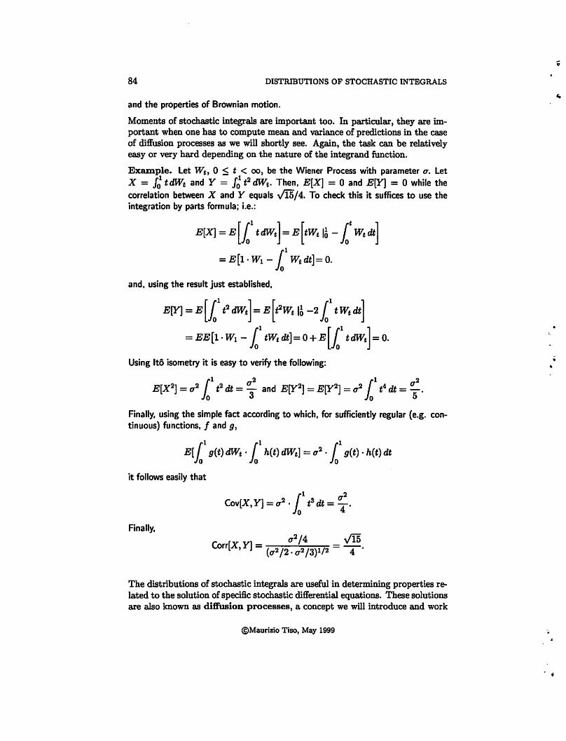
84 DISTRIBUTIONS OF STOCHASTIC INTEGRALS
and the properties of Brownian motion.
Moments of stochastic integrals are important too. In particular, they are important when one has to compute mean and variance of predictions in the case of diffusion processes as we will shortly see. Again, the task can be relatively easy or very hard depending on the nature of the integrand function.
ExBinple. Let Wt, 0 :5 t < oo, be the Wiener Process with parameter u. Let X = It t dWt and Y = It t2 dWt. Then, E[X] = 0 and E[Y] = 0 while the correlation between X and Y equals ../15/4. To check this it suffices to use the integration by parts formula; i.e.:
E[X) = E[[ tdWc]= E[tw,IA-l Wcdt] = E[l · W1 - [ Wcdt]= 0.
and, using the result just established,
E[Y) = E[[ t2dWc]= E[t2w, IA-2 [ tWcdt] =EE[l·W1 - [ tWcdt]=O+E[[ tdWc]=o.
Using Ito isometry it is easy to verify the following:
1
1 u2 11 q2 E[X2
] = u2 t2 dt = - and E[Y2] = E[Y2] = u2 t4 dt = - . 0 3 0 5
Finally, using the simple fact according to which, for sufficiently regular (e.g. continuous) functions, f and g,
E([ g(t) dWc · [ h(t) dWc] = u2 • [ g(t) · h(t) dt
it follows easily that
11 q2
Cov[X,Y]=u2 · 0
t3 dt= 4 .
Rnally, q2/4 v1Is
Corr[X, Y] = (u2 /2. q2 /3)1/2 = 4·
The distributions of stochastic integrals are useful in determining properties related to the solution of specific stochastic differential equations. These solutions are also known as diffusion processes, a concept we will introduce and work
©Maurizio Tiso, May 1999
0

..
Cl
• ' .
STOCHASTIC INTEGRATION: ITO INTEGRAL 85
with in a different set of notes, and are a special class of stochastic processes. Not too surprisingly, Brownian motion is the basic ingredient in deriving several other stochastic processes which have proved useful in applications.
Example. The arithmetic Brownian motion with drift a and volatility u which can be defined as a stochastic differential, i.e.:
dXt = adt + udWt.
This process has the following properties:
(1) X may be positive or negative.
(2) If u > t, then Xu is a future value of the process relative to time t. The distribution of Xu given Xt is normal with mean Xt + a( u - t) and standard deviation uJu - t.
(3) The variance of the forecast Xu tends to infinity as u does (given t,Xt).
To show that the second statement about Xu given Xt is correct, it suffices to write Xu as
Xu=X,+a lu dt+t1 lu dWt
and use the fact that ft dWt r.J N(O,u -t). Example. The geometric Brownian motion with drift a and volatility u is a stochastic process whose stochastic differential is given by
dXt = aXt dt + uXt dWt.
It has the following properties:
(1) If X starts at a positive value, it will remain positive. In particular, Xt -+ oo a.s. as t -+ oo if .X > u2 /2, Xt -+ 0 a.s. as t -+ oo if .X < u2 /2 and Xt keeps oscillating between O and oo as t -+ oo if .X = u2 /2.
(2) X has an absorbing barrier at 0.
(3) Xt I X 8 is lognormally distributed with mean X 8 • ea(t-s) and variance X!e2a(t-s) • (e0'2 (t-s) - 1). This shows that both the mean of the forecast tend to zero when a< 0 and to infinity when a> 0. Similarly, the variance of the forecast tends to infinity as t does when a ~ u2 /2 and to zero when a< u2/2.
(4) The variance of the forecast Xu tends to infinity as u does.
Property (1) is not evident. But, if one assumes that X0 is positive and solves the stochastic differential equation, the solution turns out to be:
Xt = Xo ·exp{at+uWt}
©Maurizio Tiso, May 1999
arithmetic Brownian motion
geometric Brownian motion

meanreverting Ornstein Uhlenbeck
86 DISTRIBUTIONS OF STOCHASTIC INTEGRALS
which is clearly always positive. Then, letting Yt = log(Xt) it is easily seen, using Ito formula, that when u2 /2-:/; ,\
Ii Yt ( u2
) 1. Wt ( u2
) m -= a-- +u un -= a--t~oo t 2 t~oo t 2
as by the law of the iterated logarithm we know that limt~oo sup ,/2t ~ log t = 1
and limt~oo inf J2t~logt = -1. If u2 /2 = A, then it is
r Yt and Ii ·nr Yt t~~supT=u t~~1 T=-u
from which the desired conclusions follow. Property (2) does not require any comment. As for property (3), if one lets Yt = ln(Xt), a simple application of Ito's formula gives that dYt = (a - (1/2)u2) dt + u dWt from which it is easily seen that
l't I Y, - N(Y,, + (a - ~)(t- s),u2(t- s)).
Finally, since Xt = exp{Yt}, we use the fact for which if a random variable Z l'J
N(µ,, u2) then V = exp{ Z} l'J Lognormal(µ,, u2) and E[V] = exp{µ, + u2 /2}, Var[V] = exp{ 2(µ, + u2
)} - exp{2µ, + u2 }.
Example. The mean-reverting Ornstein-Uhlenbeck process can be written as a stochastic differential of the form
dXt =a(Xt -m)dt+udWt, a< 0.
(1) X maybe positive or negative.
{2) The conditional distribution of Xu given X 0 is normal with mean given by m + (Xo - m)eau and standard error J~2a • v'(l - e2au).
(3) The variance of Xu I Xo is increasing in u but tends to a finite number as u goes to infinity; the average of Xu I X0, on the other hand is decreasing in u and tends tom as u goes to infinity.
The normality of the distribution of Xu follows easily from the normality of J; dW8 •
To compute the mean and variance of this distribution the following technical trick can be used. Let Xu = Que-u+m. Then, Ito's formula gives dXu = -Que-u du+ e-u dQu = (m - Xu) dt + e-u dQu. Since the drift terms match, one can compare the volatility terms, i.e. it must be u dWu = e-u dQu which implies that dQu = ueu dWu. Simple algebraic manipulations give then
Xu = m + (Xo - m)e-u + u fou e•-u dW,.
From this expression, it is easy to compute the mean and variance of the process. In fact, since E[J
0u es-u dW8 ] = 0 and E[J
0u es-u dW8 ]2 = J; e2Cs-u) dt using
properties of Ito integrals.
©Maurizio Tiso, May 1999
;.
0 -; .;

"
IP
•
p
0
STOCHASTIC INTEGRATION: ITO INTEGRAL 87
Figure 1.4: Left. Mean reverting Oernstein-Uhlenbeck process with Xo = 2.3, m = 2, u = .5 and a = -1.0. Superimposed to the plot are the mean function and the 95% pointwise confidence interval for Xu I Xt when t = 1.2 and u E (1.2,2). Right. Geometric Brownian motion with Xo = .1, a = .3, u = .1. Superimposed to the plot are the mean function and the 95% pointwise confidence interval for Xu I Xt when t = 1 and u E (1, 2).
Remark. Mean reverting processes are found to be appropriate for modeling interest rates when they are known to have stable long-run values. Sometimes, volatility of stock prices is also modeled as a mean reverting process. A good introduction to modeling stochastic interest rate through diffusion models is available in Shiryaev (1999), chapter 3 section 4. A good reference for applications of such models is Rebonato (1996).
Example. This example is a little bit more difficult. We want to determine the distribution of Xt I X 8 when Xt is known to satisfy the following stochastic differential:
dX1 = (2.ax1 + U:) dt+uJx;dW1,
A simple inspection of the differential does not suggest an easy answer. However, there is a general result that we are going to use and, namely, if
dX1 = (.8o(X1)h(X1) + ~ g(X1)g' (X1)) dt + ug(Xt) dW1 (1.70}
where h(x) = r 91~ and h has an inverse, then the solution of (1.70) is given by
X1 = h-1 ( e111 h(Xo) + u 1' e-ll• dW,).
This can be proved very easily if, starting from (1.70), we let Yt = h(Xt)- In fact,
©Maurizio Tiso, May 1999

88 DISTRIBUTIONS OF STOCHASTIC INTEGRALS
Ito's formula gives then
( 1 u2 1
dYt = {Jg(xt)h(Xt) g(Xt) + 2 u(Xt)U' (Xt) g(Xt)
-11; g2(Xc) ;:~1D dt + ( ag(Xc) uciJ dWt = ,8Yt dt + adWc,
The last stochastic differential equation has the solution
Yt = ellt(Yo+a LT e-11•dW.)
which can be verified using again Ito's formula. Anally,
Xt = h-1(Yt) = h-1 (ellth(Xo) + 11 [ e-11• dW.).
The original stochastic differential can be written as in (1. 70) if we let g(Xt) = ../Xi (and this automatically implies that h(Xt) = 2../Xi). Thus, we have that the solution of the original equation is given by
Xe = ( e211\/Xc;-+ 17 Lt e-211• dW. r, As we already know, J: e-2/Js clWs r-J N(O, J: e-4/Js dt, i.e. N(O, 4~ (1- e-4/Jt), so it is easily checked that, when Xo is given and nonnegative,
e•11t ../Xo + a Lt e-•11• dW, ~ N ( e•llt ../Xo + :; (1 - e-411t) )
This implies that
2/3e4Ptxo Xt I Xo r-J t'{1,o) where 6 = u2 (1 - e-4/Jt).
Using properties of the non-central chi-squared distribution, it is also found that
4{3e4/Jt Xo 16/3e4/Jt Xo E[Xt I Xo] = 1 + u2 (l _ e-4/Jt) and Var[Xt I Xo] = 2 + u2 (l _ e-4/Jt)
which shows that both the forecast and its standard error go to infinity as t does.
Example. The following Ito stochastic differential
dXt = 1 dt + 2,Jx;, clWt
is not so easy to find the distribution for. But, we know that a solution Xt to the previous stochastic differential equation is also a solution to the following FiskStratonovich stochastic differential equation (1.53)
dXt = 0 dt + 2,Jx;, 0 clWt.
©Maurizio Tiso, May 1999
a Cl
a
"

9
"
STOCHASTIC INTEGRATION: ITO INTEGRAL 89
This is equivalent to Xt112dXt = 2 o Wt whose solution is easily seen to be 2~ = 2../Xo + 2Wt or Xt = ( ../Xo + Wt)2 and hence Xt I X 0 is distributed as a noncentral chi-squared r.v. with noncentrality parameter 2X6 /t. Modern financial theory, derivative theory in particular, is based on the random movements of financial quantities. Deterministic equations for the values of these quantities can be derived when the building block is the Wiener process. Unfortunately, deterministic equations are seldom satisfactory in describing how the future values of financial quantities will evolve. For example, what is the probability of a call or put option to expire in the money? Deterministic equations can tell us a few things about the values of these options but not about their probability to expire in the money. Diffusion models, transition probabilities density functions, first exit times and steady state distributions are the right tools for this kind of problems.
The few examples above have shown how to find the distributions of some diffusion processes. Our. approach has been that of explicitly solving the Ito stochastic differential equations (more properly, stochastic integral equations) that are used to define them. Unfortunately, this is possible for a small number of cases only. To compute the distributions for general diffusion processes one needs to use a different approach, namely, the general theory of Markov processes, and Kolmogorov backward and forward equations. Wilmott (1998), chapter 10 is a suitable first introduction to this type of problems.
Using Girsanov Theorem and its generalizations (Liptser, Shiryaev (1977), chapter 6) and the absolute continuity of measures corresponding to Ito processes and processes of diffusion type (Liptser, Shiryaev (1977), chapter 7) one can compute the characteristic functions of quadratic or bilinear functional of the Brownian motion. This fact has important implications when dealing with the statistical properties of regression models for nonstationary time series. Several important examples relative to the distribution of quadratic functionals of Brownian motion and Ornstein-Uhlenbeck processes are available in Tanaka's (1996) book.
©Maurizio Tiso, May 1999

90 REFERENCES
13. References
Borkar, V. S., Probability Theory. An Adt1anced Oourse, Springer 1995.
Brockwell, P. J, Davis, R. A., Introduction to Time Series and Forecasting, Springer, 1996 (Section 10.4 contains an introduction to continuous-time models)
Fleming, T. R., Harrington, D. P., Oounting processes and sun1it1al analysis, Wiley, 1991.
Folland, G. B., Real Analysis, Modem Techniques and its Applications, Wiley 1986.
Friedman, A., Stochastic Differential Equations and Applications, Vol. I, Acadeinic Press 1975.
Hamilton, J. D., Time Series Analysis, Princeton University Press, 1994
Harrison, J.M., Pliska, S. R., Martingales and Stochastic Integrals in the Theory of Oontinuous Trading, Stochastic Processes and their Applications, 11 (1981) 215-60.
Harrison, J. M., Pliska, S. R., A Stochastic Model of Oontinuous 'lrading, Stochastic Processes and their Applications, 15 (1983) 313-6
Jones, F., Lebesgue Integration on Euclidean Space, Jones and Bartlett, 1993.
Kallianpur, G. Stochastic Filtering Theory, Springer 1980.
Klebaner, F. C., Introduction to Stochastic Oalculus with Applications, Imperial College Press 1998.
Kloeden, P. E., Platen, E., Numerical Solution of Stochastic Differential Equations, Springer, 1992.
Liptser, R. S., Shiryaev, A. N. Statistics of Random Processes I. General Theory, Springer and Verlag 1977.
Mao, X., Stochastic Differential Equations and their· Applications, Horwood Pub., 1997.
0l<sendal, B., Stochastic Differential Equations, ,4th Edition, Springer 1995.
Protter, P., Stochastic Integration and Differential Equations, Springer 1990.
Rebonato, R. Interest-Rate Option Models. Understanding, Analysing and Using Models for Exotic Interest Rate Options, Wiley 1996
Shiryaev, A. N., Essentials of Stochastic Finance. Facts, Models, Theory, World Scientific Publishing Co. 1999
Tanaka, K., Time Series Analysis; Nonstationarity and Nonint1ertible Distribution Theory, Wiley 1996
Todorovic, P., An Introduction to Stochastic Processes and Their Applications, Springer-Verlag 1992.
Wilmott, P., Derit1atit1es. The Theory and Practice of Financial Engineering, Wiley 1998
©Maurizio Tiso, May 1999
a
,._