lecture note #4-1
TRANSCRIPT

Lecture Note #4-1 IIT Kharagpur 2019 1st Semester
Short Course
Design of Aircraft Components using Composite Materials
787 Dream Liner
Eurofighter Typhoon
Indian Institute of Technology-Kharagpur Department of Aerospace Engineering
Professor Changduk Kong

Part 3-1
Calculation Example
A. Laminate calculations - Using : Laminate analysis
Netting rule 10% rule Carpet plots B. Panel buckling calculations
- Using : Laminate analysis/ESDU C. Thin wall section calculations
- Using : Laminate analysis / thin-wall analysis Appendix
A. Laminate solutions B. Panel buckling solutions C. Thin wall section solutions D. Data
4-1

A4.1 Laminate design for given loads
Givens : • Membrane ultimate loading intensities from a preliminary analysis as illustrated below
• Material UD-HSCFEP/ stress free temperature 120℃
• Ply thickness 0.125mm
Design:
-An efficient laminate to carry the given loads at 20℃ working
temperature 1. Perform a netting laminate analysis for preliminary sizing 2. Check and refine by running a classical laminate analysis
(ⅰ)Using a quasi-isotropic laminate design (QI)
(0,±45,90 standard angles)
(ⅱ)Using a principal stress design (PS)
( θ± in the direction of the calculated principal stresses)
mmN500N
mmN1000N
mmN2000N
xy
y
x
=
−=
=
• Neglect thermal effect

Check: . Effective limit strength
. Effective ultimate strength . Stiffness coupling terms . Engineer elastic constants . Effects of temperature Compare : QI and PS designs *Note:
. QI design : Use laminate netting rule to make an initial estimate of the required . 0,90,±45 laminate to carry the given
xyyx NNN loading
. Principal Stress Design : Using laminate netting rule to make an initial estimate of the required θ± laminate to carry the
111 NN principal loading
. For given xyyx NNN loading the principal load intensities are
given by:
xyyxyx NNNNNN 221 4)(
21)(
21
+−++=
xyyxyx NNNNNN 2211 4)(
21)(
21
+−−+=
)(21
yxxy NNN +=
where yx
xyp NN
N−
= − 2tan
21 1θ
Nxymax 𝑁𝑁𝑥𝑥𝑥𝑥𝑥𝑥𝑥𝑥𝑥𝑥=12
(𝑁𝑁𝐼𝐼 − 𝑁𝑁𝐼𝐼𝐼𝐼)

*Note by definition: shear stress will be zero on the pθ± principal
axis Advantages:
. More efficient(less plies needed) Disadvantages:
. Significant 2616 AA shear coupling terms large passion ratio
Failure analysis . Effective design limit strength ≡ first 2-2or 1-2matrix failure
i.e. : First ply failure “FPF” considered as a partial ply failure with arbitrary stiffness degradation factors applied to matrix dominated properties
→→
1212
2222
1.01.0
GGEE Reasonable first estimate
. Effective design ultimate strength ≡ first 1-1 firbre failure i.e. : Last ply failure “LPF”
due to large Poission ratio

→ mmNt x 33.115002000
*1
==≥σ
→ 64.10125.033.1
==≥pt
tt : Try 12 ⅹ0°
*190
σσ ≤=t
N xx
→ 83.012001000
*190 =
−−
=≥σ
yNt : → 8 ⅹ90°
*145
σσ ≤=t
N xyxy
→ → 42.01200500
*145 =
−=≥
σxyN
t : → 4ⅹ+45°
or 4ⅹ-45° Use Lower of ten. or comp.
strength values
Ny
Laminate Calculation Example A4.1
A 4.1 (ⅰ) QI Laminate Design 0,±45,90°
Netting Analysis:
For xN , Design for *1σσ ≤=tN x
x
No. of plies
mmN500N
mmN1000N
mmN2000N
xy
y
x
=
−=
=HW # 4
No. of plies ≥ 𝑡𝑡90𝑡𝑡𝑝𝑝
= 0.830.125
=
6.64 ∶ 𝑡𝑡𝑡𝑡𝑡𝑡 8 𝑥𝑥 90𝑜𝑜
No. of plies ≥ 𝑡𝑡45𝑡𝑡𝑝𝑝
= 0.420.125
=
3.36 ∶ 𝑡𝑡𝑡𝑡𝑡𝑡 4 x +45o for ten. and 4 x -45o for comp.

→ Initial QI laminate: 12ⅹ0° , 8ⅹ90°, 4ⅹ(+45°), 4ⅹ(-45°)
i.e. ∑ = 28 ply laminate = 3.5mm total thickness
For stacking sequence consider scheme layup guide lines; E.g. (+45, -45, 0, 90, 0, 90 , 0 , +45 ,-45 , 0, 90, 0 , 90 , 0)s
i.e. : { }[ ]s22 0,)90,0(,45±
Check strength by CLT (CCD program)
mmN500N
mmN1000N
mmN2000N
xy
y
x
=
−=
=

Check strength of QI design by CLT (CCD program)

Check strength of QI design by CLT (CCD program)

A 4.1(ⅱ) PS Laminate Design 22 5004)10002000(
21)10002000(
21
×+++−=IN
= 500 +1581 = 2081 N/mm
ΙΙN = 500=1581 = -1081N/mm
)10812081(21
+=MAXXYN
=1581N/mm
)(tan10002000
5002
2
1 1
××
= −pθ
= 9.22° i.e. ΙN @9.22°, ΙΙN @99.2° Netting Analysis
For ΙN , Design for *12.9
σσ ≤=t
NII
→ 39.115002081
*12.9 ==≥
σINt mm : Try 12plies.
+

For ΙΙN , Design for *12.99
σσ ≤= ΙΙΙΙ
tN
@99.2°
→ 90.012001081
*12.99 =
−−
=≥ ΙΙ
σNt mm : Try 8plies.
i.e. 12plies @ 9.2°, 8plies @99.2°
∑ 20plies = 2.5mm total laminate thickness
Stacking sequence ? Try : (9,99,9,99,9,9,99,9,99,9)s
i.e. ( )[ ]2222 9999999 ),(,,, S

Check strength of PS design by CLT (CCD program)

Check strength of PS design by CLT (CCD program)
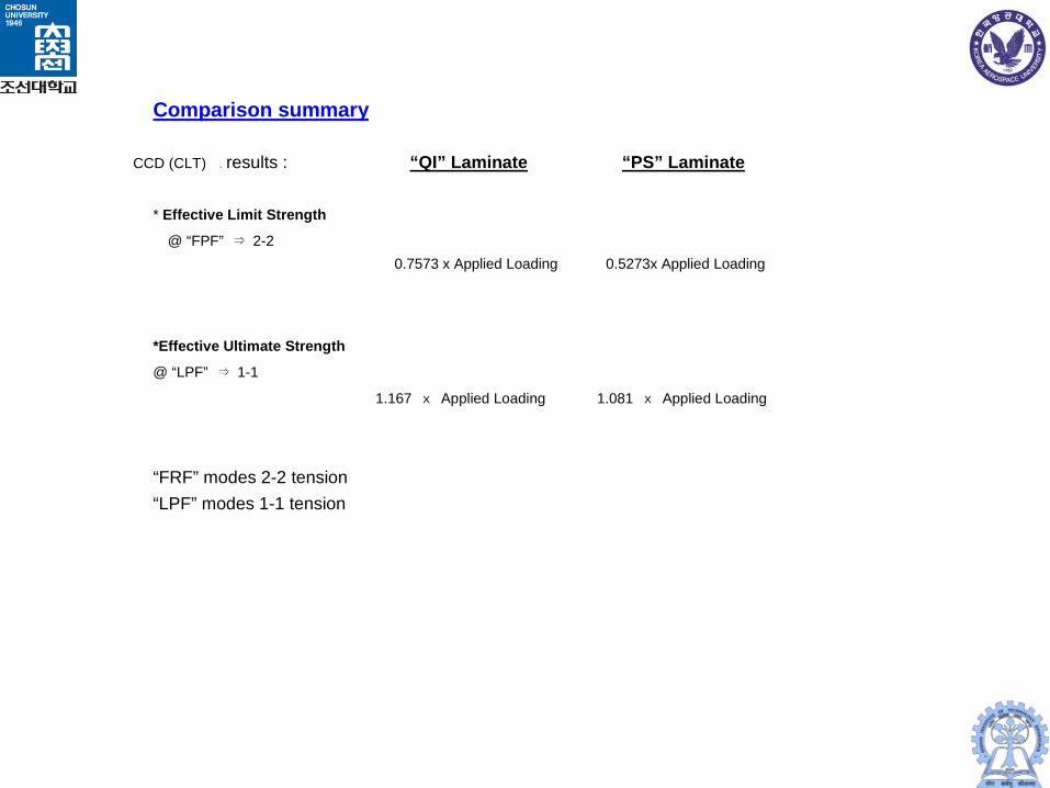
Comparison summary Lam 14a results : “QI” Laminate “PS” Laminate * Effective Limit Strength
@ “FPF” ⇒ 2-2
∆T =100℃ 0.254 ⅹ Applied Loading 0.227 ⅹ Applied Loading
∆T = 0℃ 0.582 ⅹ applied Loading 0.518 ⅹ Applied Loading
*Effective Ultimate Strength
@ “LPF” ⇒ 1-1
∆T =100℃ 1.167 ⅹ Applied Loading 1.081 ⅹ Applied Loading
∆T = 0℃ 1.163 ⅹ Applied Loading 1.074 ⅹ Applied Loading
“FRF” modes 2-2 tension “LPF” modes 1-1 tension
0.7573 x Applied Loading
CCD (CLT)
0.5273x Applied Loading

A5.Comparison of laminate analysis methods Compare the stiffness and strength values predicted by : 1) Laminate analysis 2) Netting rule 3) Hart-smith 10% rule 4) Carpet plots for cross ply, angle ply and quasi-isotropic laminates *Note: • For material data values use quasi-isotropic laminates
1) – 3) representing unfactored mean material values
• Use carpet plot data values for specific “HS carbon/epoxy” material2 with degraded properties measured at 120℃ and 1% moisture
in method 4) • The results for carpet values are expected to be lower since degraded • Degraded property predictions can be obtained from methods 1)-3)
by using factored mean values.

E.g. : typical reduction factors for strength related design include; 1.2 for material property
1.1 for service degradation
giving a compounded factor of 1.45
1.1 for thermal effects • Dividing input data values or predicted results by these factors provides a method of allowing for degradation effects in method 1-3

0%(Netting) Rule for laminate stiffness or strengths Loading Stiffness %ply contribution factor Apply to Strength 0° ±45 90° xE 1.0 0 0 1E
yE 0 0 1.0 1E
xyG No prediction of off-axis stiffness
Uni-axial xσ 1.0 0 0 *1σ longitudinal
Uni-axial yσ 0 0 1.0 *1σ
Transverse
Bi-axial xyτ 0 1.0 0 *1σ
Equal/opposite sign i.e. pure shear × RoM ply thickness fraction
t
t 0 t
t 45 t
t 90
Note 45t = 2/45±t

10% Rule for laminate stiffness Loading Stiffness % ply contribution factor Apply to 0° ±45° 90° xE 1.0 0.1 0.1 1E YE 0.1 0.1 1.0 1E
xyG 0.1 0.55 0.1 *)1(2
1
vE+
x RoM ply thickness fraction
t
to t
t 45± t
t 90
……………………………………………………………………………………………
xyv for QI laminates
±
+
=
45%90%41
1
i.e. with plies in all 0°,±45°, 90° directions
where *v is the poisson ratio of the “complimentary layup” for doubly symmetric laminates, e.g.:
for ±45° *v = 45±v =0.05
for 0°,90° *v = 90,0v =0.8 for 0°, ±45°,90° *v = 90,45,0 ±
v =0.33

10% Rule for laminates strengths 17 *Note, here layer contribution factor also depends on loading system Loading Strength % ply contribution factor Apply to 0° ±45° 90° Uniaxial x*σ 1.0 0.1 0.1 *1σ
yσ 0.1 0.1 1.0 *1σ
Bi-axial x*σ 1.0 0.55 0.1 *1σ Same sign
y*σ 0.1 0.55 1.0 *1σ
Bi-axial
Opposite sign xy*τ 0.1 0.55 0.1 2/*1σ
i.e. Shear x RoM ply thickness fraction
t
t 0 t
t 45± t
t 90
𝜎𝜎∗y

LAMINATE CALCULATION EXAMPLE A.5 ( i ) Cross Ply LAMINATE
- Laminate ( )S90,0 UDHSCFEP, 0.5mm thick Stiffness
xE : Laminate analysis transformed layer stiffness
● LAM 14A → laminate equivalent value = 75.4 GPa
● Netting Rule :
9045
0
000014050
125021 )()(
..
×+×+×
×
×±
etc = 70
● H.S. 10% rule:
( ) 1405.0125.021.001.0140
5.0125.021
9045
0
×
×
×+×+×
×
×±
etc = 77
● Carpet plot read off modulus for
REF 2 50% 0° 0%±45° 50%90° =67*
yE : Laminate analysis: transformed layer stiffness
LAM 14a → laminate equivalent value = 75.4
● Netting Rule :
1405.0125.021)0(0
5.0125.020
9045
0
×
×
×+×+
×
×±
etc = 70
● H.S 10%rule:
( ) 1405.0125.02101.0140
5.0125.021.0 45
0
×
×
×+×+×
×
×±
etc = 77
● Carpet plot read off modulus for
REF 2 50%0° 0%±45° 50%90° =67*
CLT
CLT

Degraded Mechanical Properties of typical Aerospace Approved HS Carbon Epoxy
Degraded longitudinal modulus (1% moisture, 120°C)
Degraded in-plane shear modulus (1% moisture, 120°C)
Degraded shear strength (1% moisture, 20°C (a) and 120°C (b))
Degraded compression strength (1% moisture, 120°C)
Degraded tensile strength (1% moisture, 120°C)

xyG : Laminate analysis transformed layer stiffness
● LAM 14A →Laminate Equivalent Value =20.6
● Netting Rule
No prediction for matrix dominated property
● H.S. 10%rule
( ) ( ) 1125.021.0
33.012140
1125.0455.0
33.012140
1125.021.0
90450
×
×
×++
×
×
×++
×
×
×±
=17.1
● Carpet plot: read off tensile strength for
REF 2 25%0° 50%±45° 25%90° =11* 2/ mmKN
140 140
20.6
= 5
=4
𝐺𝐺𝑥𝑥𝑥𝑥=0.1 2×0.1250.5 0° ×
1402(1+0.8)
+0.55× (0)±45°𝑒𝑒𝑡𝑡𝑒𝑒 + 0.1 × (2×0.1250.5
)90° ×140
2(1+0.8)=3.89
CLT

(ii) Cross Ply Laminate - ( )S90,0 UDHSCFEP, 0.5mm thick Strength
*xσ : Laminate analysis transformed layer strength
● LAM 14A →1-1 Last Ply Failure @ xσ =379.4/0.5 =759
● Netting Rule
( ) ( )
9045
0
0000150050
125021 etcetc ×+×+×
×
×±.
. = 750
● H.S 10% rule: ( ) 15005.0125.021.0055.01500
5.0125.021
9045
0
×
×
×+×+×
×
×±
etc
=825
● Carpet plot READ OFF TENSILE STRENGTH FOR
REF 2 50%O° 0%±45° 50%90° = 600 2/ mmN
*yσ : Laminate analysis transformed strains/max strain criteria
● LAM 14A →1-1 Last Ply Failure @ yσ =3.79.4/0.5 =759
● Netting Rule
( ) ( ) 150050
1250200000
904590×
×
×+×+×± etcetcetc
..
= 759
● H.S 10%rule
( ) 15005.0125.021055.01500
5.0125.021.0
9045
0
×
×
×+×+×
×
×±
etc =825
● Carpet plot: read off tensile strength for
REF 2 50%O° 0%±45° 50%90° =600 2/ mmN
1 750
CLT
CLT
layer strength
1
1

xyτ : Laminate analysis transformed strains/max strain criteria
● LAM 14A →1-2 First Ply Failure @ xσ =35/0.5 =70
● Netting Rule
No prediction for matrix dominated properties
● H.S 10%rule
( )2
15005.0125.021.0055.0
21500
5.0125.021.0
9045
0
×
×
×+×+×
×
×±
etc =75
● Carpet plot: read off tensile strength for
REF 2 50%0° 0%±45° 50%90° =45* (70RT) 2/ mmN
CLT 𝜏𝜏xy = 35/0.5 =70
layer strength

( i ) Angle Ply Laminate - Laminate ( )S45± UDHSCFEP, 0.5mm thick
xE : Laminate analysis transformed layer stiffness
● LAM 14A → Laminate Equivalent Value = 17.7
● Netting Rule
No prediction for matrix dominated laminate
● H.S 10%rule
( ) ( )
9045
0010140
50
125041001 etcetc ×+×
×
×+×±
.... = 14
● Carpet plot: read off tensile strength for
REF 2 0%0° 100%±45° 0%90° =15* 2/ mmKN
yE : Laminate analysis transformed layer stiffness
● LAM 14A → Laminate Equivalent Value = 17.7
● Netting Rule
No prediction for matrix dominated laminate
● H.S 10%rule
( ) ( )
9045
001140
50
1250410010 etcetc ×+×
×
×+×±.
... =14
● Carpet plot: read off tensile strength for
REF 2 0%0° 100%±45° 0%90° =15* 2/ mmKN
CLT
CLT

xyG : Laminate analysis transformed layer stiffness
● LAM 14A → Laminate Equivalent Value = 36.2
● Netting Rule
No prediction for matrix dominated property
● H.S. 10%rule
( )( )
( )
045
0001
05012
140
50
12504550010 etcetc ×+
+×
×
×+×±
...
... =36.7
● Carpet plot: read off tensile strength for
REF 2 0%0° 100%±45° 0%90° =32* 2/ mmKN
* Degraded Carpet Plot Values
(ii) Angle Ply Laminate - Laminate ( )S45± UDHSCFEP, 0.5mm thick
*xσ : Laminate analysis transformed strain/max strain criteria
● LAM 14A →1-2 First Ply Failure @ xσ =70/0.5 =140
● Netting Rule
No prediction for matrix dominated laminate
● H.S. 10%rule
( ) ( )
9045
0 01.015005.0125.041.001 etcetc ×+×
×
×+×±
=150
● Carpet plot: read off tensile strength for
REF 2 0%O° 100%±45° 0%90° =150* 2/ mmN
0.1
CLT
CLT
layer strength

*yσ : Laminate analysis transformed strain/max strain criteria
● LAM 14A →1-2 First Ply Failure @ xσ =70/0.5 =140
● Netting Rule
No prediction for matrix dominated laminate
● H.S 10%rule
( ) ( )
9045
0 0115005.0125.041.001.0 etcetc ×+×
×
×+×±
=150
● Carpet plot: read off tensile strength for
REF 2 0%O° 100%±45° 0%90° =150* 2/ mmN
*xyσ : Laminate analysis transformed strain/max strain criteria
● LAM 14A →2-2 First Ply Failure @ xσ =181/0.5 =362
● Netting Rule
No prediction for matrix dominated property
● H.S 10%rule ( ) ( )
9045
0 01.02
15005.0125.0455.001.0 etcetc ×+×
×
×+×±
= 412.5
● Carpet plot: read off tensile strength for
REF 2 0%0° 100%±45° 0%90° =350* 2/ mmN
* Degraded Carpet Plot Values
CLT
CLT
layer strength
layer strength
𝜏𝜏xy

( i ) Quasi Isotropic Laminate - Laminate ( )S90,45,0 ± UDHSCFEP, 1mm thick
xE : Laminate analysis transformed layer stiffness
● LAM 14A →LAMIANTE EQUIVALENT VALUE =54.1
● Netting Rule
9045
0
)0(0)0(01405.0125.021 etcetc ×+×+×
×
×±
= 35
● H.S. 10%rule
1401
125.021.01401
125.041.01401
125.0210
×
×
×+×
×
×+×
×
×
=45.5
● Carpet plot; read off tensile strength for
REF 2 25%0° 50%±45° 25%90° =42* 2/ mmKN
yE : Laminate analysis transformed layer stiffness
● LAM 14A →Laminate equivalent value =54.1
● Netting Rule
( ) 1401
125.021)0(00090
450 ×
×
×+×+×±
etcetc = 35
● H.S 10%rule
1401
125.0211401
125.041.01401
125.0210
×
×
×+×
×
×+×
×
×
=45.5
● Carpet plot : read off tensile strength for
REF 2 25%0° 50%±45° 25%90° =42* 2/ mmKN
0.1
1
CLT
CLT

xyG : Laminate analysis transformed layer stiffness
● LAM 14A →Laminate Equivalent Value =20.6
● Netting Rule
No prediction for matrix dominated property
● H.S. 10%rule
( ) ( ) 1125.021.0
33.012140
1125.0455.0
33.012140
1125.021.0
90450
×
×
×++
×
×
×++
×
×
×±
=17.1
● Carpet plot: read off tensile strength for
REF 2 25%0° 50%±45° 25%90° =11* 2/ mmKN
(ⅱ) Quasi Isotropic Laminate - Laminate ( )S90,45,0 ± UDHSCFEP, 1mm thick
*xσ : Laminate analysis transformed layer strength
● LAM 14A →1-1 Last Ply Failure @ xσ =558/1 = 558
● Netting Rule
9045
0
)(0)(015005.0125.021 etcetc ×+×+×
×
×±
= 375
● H.S 10%rule 15001
125.021.015001
125.041.015001
125.0210
×
×
×+×
×
×+×
×
×
=487
● Carpet plot: read off tensile strength for
REF 2 25%0° 50%±45° 25%90° =380 2/ mmN
1402(1 + 0.33)
17.1
CLT
CLT
1402(1 + 0.33)
374

*yσ : Laminate analysis transformed strains /max strain criteria
● LAM 14A →1-1 Last Ply Failure @ xσ = 558/1 = 558
● Netting Rule
( ) 15001
125.021)0(00090
450 ×
×
×+×+×±
etcetc = 375
● H.S 10%rule
15001
125.02115001
125.041.015001
125.021.0450
×
×
×+×
×
×+×
×
×±
= 487
● Carpet plot read off tensile strength for
REF 2 25%0° 50%±45° 25%90° =380 2/ mmN
*xyτ : Laminate analysis transformed strains / max strain criteria
● LAM 14A → 2-2 First Ply Failure @ xσ = 206/1 = 206
● Netting Rule
No prediction for matrix dominated property
● H.S 10%rule
2
15001
125.021.02
15001
125.0455.02
15001
125.021.090450
×
×
×+×
×
×+×
×
×±
=243
● Carpet plot: read off tensile strength for
REF 2 25%0° 50%±45° 25%90° =110* (150 RT) 2/ mmN
CLT
CLT
𝞂𝞂y = 374
𝜏𝜏xy = 289
layer strength
layer strength

B. Panel buckling calculations Using : Laminate analysis / ESDU B1.1 Laminated plate buckling check
Given :
• Quasi-isotropic laminate (±45,0,90) sl3
• Material UD-HSCFEP/ stress free temperature 120℃
• Ply thickness 0.125mm • ESDU buckling curve
• Minimum working temperature of 0℃
• Panel dimensions 1000x250mm • All edges simply supported • Subjected to :
(ⅰ) direct compressive loading (ⅱ) pure shear loading
• Neglect thermal effect
/

Assess : - The laminate panel buckling strength for loading cases a) and b),
and compare with the laminate first ply and last ply failure strengths and also with the buckling strength of a light alloy panel of equal dimensions.
*Note: - Make use of results from a unit loading laminate analysis run - Use derived flexural stiffness terms for buckling calculations

(ⅰ) direct compressive loading (ⅱ) pure shear loading
Appendix B. Panel buckling solutions B1 (ⅰ) Uniaxial Compression Loading Laminate Analysis
- Using unit xN load intensity - Derived bending stiffness values from Lam 14a
( )21
2211DD = 125687 Nmm ( )6612 2DD + = 161058 Nmm = “ D ”
( )41
1122 /DD = 0.97 Nmm *Note laminate strength values for Compression
First Ply failure occurs @ xN = -886 mmN / in mode 2-2/T, layer 4 “FPF” i.e. @ xσ =-886/3=-295 2/ mmN Last ply failure @ xN =-1346 mmN / in mode 1-1/T, layer 3
i.e. @ xσ =-1346/3=-449 2/ mmN Buckling calculation – using ESDU
4250
1000==
ba
88.397.0441
11
22 =×=
DD
ba → Asymptote value
Ends/sides simply supported → c=2 ESDU Fig.1 → 0k =20
CLT

Dij : in order to match the unit as N-mm, 109 times must be applied to these values

Aspect ratio=a/b=1000/250=4 K’=4 from graph “SS-SS” case K=4x0.904=3.62
( ) ( )2
66122
222110
Xcrit b2DDCΠ
bDDKN +
+=
2
2
2 250058'1612
250678'12520 ×Π
+×
=
87.5022.40 += mmN /09.91=
→ 309.91
=Xcritσ =30.36 mmN / Note <<FPF
Compression with Al alloy panel of equal thickness 2
=
btKExyσ
2
2503000'7062.3
×=
=36.5 2/ mmN *Note : Compression panel direct Compression buckling strength
= 83% of ally panel buckling strength!
2
cr
Buckling occurs!
Composite

• Depending on support B.C.,
different K=K’
Fig. 12.7
A: F-F B: F-S.S C: S.S-S.S D: F-Free E: S.S.-Free
Loading ends: S.S Loading ends: F(fixed)
Loading end side
Side’s B.C.

B1(ⅱ) Pure in-plane shear loading
Laminate Analysis
- Using unit xyN load intensity
- Bending stiffness as for run A3.1(ⅱ) - Laminate strength values for comparison
First ply failure occurs @ xyN = 210 mmN / in mode 2-2/T, layer 2(-45°)
i.e. @ 2N/mm 703
210==xyτ
Last Ply Failure occurs @ mmNNx /927= in mode 1-1/T, layer 2(-45°)
i.e. @ 2/3093
927 mmNxy ==τ
Buckling Calculation – using ESDU ( ) 1610582
66110=+= DDD*
88.3*21
11
22 =
DD
ba ,
( )28.1
125687161058
21
2211
2 ==⋅DD
D
ESDU Fig 5 All edges simply supported
→ ( )
10521
2211
=⋅
⋅
DD
baNbxy xycritbxy
NN =
(ⅰ) direct compressive loading (ⅱ) pure shear loading
309
309/3=103
D0

→ ( )baDDNbxy ⋅
=21
2211105
2501000687'125105
××
=
i.e. mmNNcritxy /8.52=
and 3
8.52=
critxyτ =17.6 2/ mmN <<FPF Buckling occurs!
Comparison with AL alloy panel of equal thickness 2
=
btKE
critxyτ
2
2503000'705
×=
= 50.4 2/ mmN *Note: composite panel shear buckling strength = 35% of AL ally panel buckling strength!

2cr )
btKE(τ =
Shear buckling coefficient of plate with different B.C.
4 sides: Fixed
4 sides: SS
5

C1.1
C1.2
HW # 5

Appendix C. Thin wall section solutions (For laminate runs see examples A2.1) THIN WALL SECTION EXAMPLE C1.1 Section details:
SQILayup )90,45,45,0(3,1 −+==
→ mmt 13,1 =
mmNEx /101.54 33,1
×=
SAPLayup )45,45(2 −+== Axial load KNFx 30= → mmt 5.02 = Thru centroid
23 /107.172
mmNEx ×=
Total section area
23001001
2005.01001
mmAi =
×+×+
×=∑
Axial stiffness can be obtained by CLT, ROM or Carpet methods. Here used CLT.
2

Effective section axial stiffness
strairNEAAE xii /1059.12101.54)1001(
107.17)2005.0(101.54)1001(
6
3
3
3
×=
×××+
×××+
×××
==∑
Equivalent isotropic section modulus
236 /1097.4110300
59.12 mmNAEA
Ei
xii ×=×==∑∑
Element axial stresses
①top flange mmNE
EA
F x
i
xx /9.128
1097.41101.54
3001030
3
331
1 =××
××
=⋅=∑
σ
②web mmNE
EA
F x
i
xx /2.42
1097.41107.17
3001030
3
332
2 =××
××
=⋅=∑
σ
③btm flange 23 /9.128 mmNx =σ - by symmetry
2
2
strain

C 2 Bending loading C2.1
Top/btm Flange laminates : QI=(0,+45,-45,90)s Web Laminates : AP=(+45,-45)s
C2.2 Top/btm Flange laminates : QI=(0,+45,-45,90)s Web Laminates : AP=(+45,-45)s
C2.1
C2.2

EXAMPLE
SQILayup )90,45,45,0(3,1 −+==
→ mmt 13,1 =
mmNEx /101.54 33,1
×=
SAPLayup )45,45(2 −+== Bending Mont mmNM /101 6Z ×=
→ mmt 5.02 = About symmetric axis
23 /107.172
mmNEx ×=
Total section area
23001001
2005.01001
mmAi =
×+×+
×=∑
Effective section axial stiffness
strainNEAAE xii /1059.12101.54)1001(
107.17)2005.0(101.54)1001(
6
3
3
3
×=
×××+
×××+
×××
==∑

Equivalent isotropic section modulus 23
6
/1097.41300
1059.12 mmNAEA
Ei
xii ×=×
==∑∑
Effective section bending stiffness (rigidity) ∑= zixiz IEEI
{ }{ }( ){ }
210
10
10
10
23
33
23
/1041.111041.51059.0
101.54
1001100101.5412/2005.0107.17
100)1100(101.54mmN×=
×+
×+
×
=
××××+
×××+
××××
=
Equivalent section isotropic second moment of area 46
3
10
10722109741
104111mm
E
IEI zixiz ×=
××
== ∑ ...
Element bending(axial) stress
①top flange mmNEE
IYM x
z
zx /5.47
1097.41101.54
1072.2100)101(
3
3
6
61
1 −=××
××××−
=⋅±=σ
②web mmNE
EI
YM xzx /5.15
1097.41107.17
1072.2100)101(
3
3
6
622
2 ±=××
××××
±=⋅±=σ
③btm flange 2/5.47 mmNxi +=σ Element loading intensities - calculate from ixixi tN ×=σ → mmN /
mm2
mm2
1
Σ

C 3 Shear loading C3.1
Top/btm Flange Laminates : QI=(0,+45,-45,90)s Web Laminates : AP=(+45,-45)s
C3.2
Top/btm Flange Laminates : QI=(0,+45,-45,90)s Web Laminates : AP=(+45,-45)s
C3.1
C3.2

Thin WALL SECTION EXAMPLE C3.1
SQILayup )90,45,45,0(3,1 −+==
→ mmt 13,1 =
mmNEx /101.54 33,1
×=
SAPLayup )45,45(2 −+== Shear load yF =10KN
→ mmt 5.02 = Thru shear centre
23 /107.172
mmNEx ×= // l to principal axis
Section total area
23001001
2005.11001
mmAi =
×+×+
×=∑
Effective section axial stiffness
∑ ×=
×××+
×××+
×××
== strainNEAAE ii /1059.12101.54)1001(
107.17)2005.0(101.54)1001(
6
3
3
3

Equivalent isotropic section modulus
236
/1097.41300
1059.12 mmNAEA
Ei
xii ×=×
==∑∑
Effective section bending stiffness (rigidity)
zixiz IEEI ∑=
{ }{ }( ){ }
210
10
10
10
23
33
23
/1041.111041.51059.0
1041.5
1001100101.5412/2005.0107.17
100)1100(101.54mmN×=
×+
×+
×
=
××××+
×××+
××××
=
Equivalent section isotropic second momrnt of area
46
3
10
10722109741
104111mm
E
IEI zixiz ×=
××
== ∑ ...
Element shear flows
E
Edsty
I
FNq xi
iz
yxyxy ii
⋅== ∫ Evaluate integral
around section ①top flange : y=constant=100 , t =constant =1
mmNdsNxyb
/...
.447
109741
101541001
10722
100003
3100
0
6=
××
⋅×××
= ∫
At b point [ ] [ ] 100000100100100100 1000 =×−⋅=s
s 0
moment

②web y=100-s , t=constant =0.5
28.5188.34.471097.41
107.17ds)s100(5.0
1072.2
100004.47N
100
03
3
6xyc=+=
××
×−×××
+= ∫
=51.28t c point 50002100100002
100 2
100
0
2
=−=
− /s
s
③btm flange –by symmetry Element shear stress ixyixyi tN /=τ
:

C 4 Torsion loading
C4.1
Flange and web Laminates : AP=(+45,-45) C4.2
Top/btm Flange laminates : QI=(0,+45,-45,90)s Web Laminates : AP=(+45,-45)s
C4.1
C4.2

THIN WALL SECTION EXAMPLE C4.1 Torsional loading
mmNM x /101 3×=
All elements : sLayup )45,45(3,2,1 −+=
→ t= 0.5mm
310717 ×= .bxE
3109.20 ×=bxyG
Effective section torsional stiffness
∑= 3
3btGGJ bxy
= { }{ }{ }
26
33
33
33
/1034.03/5.0100109.2013/5.0200109.201
3/5.0100109.201mmN×=
××××+
××××+
××××
Rate of twist
mmradGJT
dxd /1087.2
10348.0101 3
6
3−×=
××
==θ
Max shear stress
233 /301087.25.0109.20max
mmNdxdtGb
xyxy ±=××××±=⋅±= −θτ
Emx

THIN WALL SECTION EXAMPLE C4.1
- Skin )90,45,45.0(3,1 −+=Layup
→ t=1mm
NEmx
3101.54 ×=
NGmxy
3106.20 ×=
- Web SAPLayup )45,45(4,2 −+==
→ t= 0.5mm Torsional loading
23 /107.17 mmNEmx ×= NmmM x
3101×=
23 /104.36 mmNGmxy ×=
Section enclosed area A=200×50=10,000 2mm 1 Effective section torsional stiffness
∫ ∑==i
mxyi
imxy tG
bA
tG
dSAGJ // 22 44
210
3
3
3
3
2 10612.1
)5.0104.36/(50)1106.20/(200)5.0104.36/(50
)1106.20/(200
/100004 Nmm×=
××+
××+
××+
××
×=
C4.2

Rate of twist
mmradGJT
dxd /10205.6
10612.1101 8
3
3−×=
××
==θ
section shear flow (constant)
mmNA
TNq xyxy /.050
100002
101
2
3
=××
===

Appendix D. Data Typical Generic Material Data For uni-directional tape and woven fabric composites
UD
Tapes Stiffness Strengths
2/ mmKN 2Nmm
(60%vf) 1E 2E 12G 12v t1σ c1σ t2σ c2σ 12τ
HSCRE
P 140 10 5 0.3 1500 -1200 50 -250 70
HMCRE
P 180 8 5 0.3 1000 -850 40 -200 60
EGFEP 40 8 4 0.25 1000 -600 30 -110 40
KFEP 75 6 2 0.34 1300 -280 30 -40 60
Typical ply thickness 0.125-0.2mm
UD
Tapes Stiffness Strengths
2/ mmKN 2Nmm
(60%vf) 1E 2E 12G 12v t1σ c1σ t2σ c2σ 12τ
HSCRE
P 70 70 5 0.10 600 -570 600 -570 90
HMCRE
P 85 85 5 0.10 350 -150 350 -150 35
EGFEP 25 25 4 0.20 440 -425 440 -425 40
KFEP 30 30 5 0.20 480 -190 480 -190 50
Typical ply thickness 0.25-0.4mm
Note : An initial estimate of strains can be made assuming linear elasticity to failure E.g. etcEtt 111 /σε =
Fabric
(50%Vf)


ESDU 80023 ESDU 80023
4
1
11
22
D
D
b
a
( )212211
0
DD
D

