lecture note - department of mathematics
TRANSCRIPT

Advanced Analysis
Min YanDepartment of Mathematics
Hong Kong University of Science and Technology
April 14, 2016
2

Contents
1 Limit of Sequence 71.1 Definition . . . . . . . . . . . . . . . . . . . . . . . . . . . . . . 81.2 Property . . . . . . . . . . . . . . . . . . . . . . . . . . . . . . . 131.3 Infinity and Infinitesimal . . . . . . . . . . . . . . . . . . . . . . 191.4 Supremum and Infimum . . . . . . . . . . . . . . . . . . . . . . 211.5 Convergent Subsequence . . . . . . . . . . . . . . . . . . . . . . 261.6 Additional Exercise . . . . . . . . . . . . . . . . . . . . . . . . . 35
2 Limit of Function 392.1 Definition . . . . . . . . . . . . . . . . . . . . . . . . . . . . . . 402.2 Basic Limit . . . . . . . . . . . . . . . . . . . . . . . . . . . . . . 482.3 Continuity . . . . . . . . . . . . . . . . . . . . . . . . . . . . . . 552.4 Compactness Property . . . . . . . . . . . . . . . . . . . . . . . 602.5 Connectedness Property . . . . . . . . . . . . . . . . . . . . . . 642.6 Additional Exercise . . . . . . . . . . . . . . . . . . . . . . . . . 72
3 Differentiation 753.1 Linear Approximation . . . . . . . . . . . . . . . . . . . . . . . . 763.2 Computation . . . . . . . . . . . . . . . . . . . . . . . . . . . . . 823.3 Mean Value Theorem . . . . . . . . . . . . . . . . . . . . . . . . 903.4 High Order Approximation . . . . . . . . . . . . . . . . . . . . . 963.5 Application . . . . . . . . . . . . . . . . . . . . . . . . . . . . . . 1043.6 Additional Exercise . . . . . . . . . . . . . . . . . . . . . . . . . 112
4 Integration 1214.1 Riemann Integration . . . . . . . . . . . . . . . . . . . . . . . . 1224.2 Darboux Integration . . . . . . . . . . . . . . . . . . . . . . . . 1314.3 Property of Riemann Integration . . . . . . . . . . . . . . . . . 1374.4 Fundamental Theorem of Calculus . . . . . . . . . . . . . . . . . 1444.5 Riemann-Stieltjes Integration . . . . . . . . . . . . . . . . . . . 1504.6 Bounded Variation Function . . . . . . . . . . . . . . . . . . . . 1574.7 Additional Exercise . . . . . . . . . . . . . . . . . . . . . . . . . 166
5 Topics in Analysis 177
3

4 Contents
5.1 Improper Integration . . . . . . . . . . . . . . . . . . . . . . . . 1785.2 Series of Numbers . . . . . . . . . . . . . . . . . . . . . . . . . . 1825.3 Uniform Convergence . . . . . . . . . . . . . . . . . . . . . . . . 1935.4 Exchange of Limits . . . . . . . . . . . . . . . . . . . . . . . . . 2035.5 Additional Exercise . . . . . . . . . . . . . . . . . . . . . . . . . 213
6 Multivariable Function 2216.1 Limit in Euclidean Space . . . . . . . . . . . . . . . . . . . . . . 2226.2 Multivariable Map . . . . . . . . . . . . . . . . . . . . . . . . . . 2286.3 Compact Subset . . . . . . . . . . . . . . . . . . . . . . . . . . . 2376.4 Open Subset . . . . . . . . . . . . . . . . . . . . . . . . . . . . . 2436.5 Additional Exercise . . . . . . . . . . . . . . . . . . . . . . . . . 249
7 Multivariable Algebra 2517.1 Linear Transform . . . . . . . . . . . . . . . . . . . . . . . . . . 2527.2 Bilinear Map . . . . . . . . . . . . . . . . . . . . . . . . . . . . . 2587.3 Multilinear Map . . . . . . . . . . . . . . . . . . . . . . . . . . . 2687.4 Orientation . . . . . . . . . . . . . . . . . . . . . . . . . . . . . . 2787.5 Additional Exercises . . . . . . . . . . . . . . . . . . . . . . . . . 285
8 Multivariable Differentiation 2878.1 Linear Approximation . . . . . . . . . . . . . . . . . . . . . . . . 2888.2 Property of Linear Approximation . . . . . . . . . . . . . . . . . 2978.3 Inverse and Implicit Differentiations . . . . . . . . . . . . . . . . 3028.4 Submanifold . . . . . . . . . . . . . . . . . . . . . . . . . . . . . 3108.5 High Order Approximation . . . . . . . . . . . . . . . . . . . . . 3188.6 Maximum and Minimum . . . . . . . . . . . . . . . . . . . . . . 3278.7 Additional Exercise . . . . . . . . . . . . . . . . . . . . . . . . . 338
9 Measure 3459.1 Length in R . . . . . . . . . . . . . . . . . . . . . . . . . . . . . 3469.2 Lebesgue Measure in R . . . . . . . . . . . . . . . . . . . . . . . 3529.3 Outer Measure . . . . . . . . . . . . . . . . . . . . . . . . . . . . 3559.4 Measure Space . . . . . . . . . . . . . . . . . . . . . . . . . . . . 3619.5 Additional Exercise . . . . . . . . . . . . . . . . . . . . . . . . . 369
10 Lebesgue Integration 37110.1 Integration in Bounded Case . . . . . . . . . . . . . . . . . . . . 37210.2 Measurable Function . . . . . . . . . . . . . . . . . . . . . . . . 37710.3 Convergence Theorem . . . . . . . . . . . . . . . . . . . . . . . . 38910.4 Convergence and Approximation . . . . . . . . . . . . . . . . . . 39510.5 Additional Exercise . . . . . . . . . . . . . . . . . . . . . . . . . 401
11 Product Measure 40511.1 Extension Theorem . . . . . . . . . . . . . . . . . . . . . . . . . 40611.2 Lebesgue-Stieltjes Measure . . . . . . . . . . . . . . . . . . . . . 413

Contents 5
11.3 Product Measure . . . . . . . . . . . . . . . . . . . . . . . . . . 41911.4 Lebesgue Measure on Rn . . . . . . . . . . . . . . . . . . . . . . 42511.5 Riemann Integration on Rn . . . . . . . . . . . . . . . . . . . . . 43511.6 Additional Exercise . . . . . . . . . . . . . . . . . . . . . . . . . 446
12 Differentiation of Measure 44912.1 Radon-Nikodym Theorem . . . . . . . . . . . . . . . . . . . . . 45012.2 Lebesgue Differentiation Theorem . . . . . . . . . . . . . . . . . 46012.3 Differentiation on R: Fundamental Theorem . . . . . . . . . . . 46512.4 Differentiation on Rn: Change of Variable . . . . . . . . . . . . 476
13 Multivariable Integration 48513.1 Curve . . . . . . . . . . . . . . . . . . . . . . . . . . . . . . . . . 48613.2 Surface . . . . . . . . . . . . . . . . . . . . . . . . . . . . . . . . 49613.3 Submanifold . . . . . . . . . . . . . . . . . . . . . . . . . . . . . 50813.4 Green’s Theorem . . . . . . . . . . . . . . . . . . . . . . . . . . 51413.5 Stokes’ Theorem . . . . . . . . . . . . . . . . . . . . . . . . . . . 52513.6 Gauss’ Theorem . . . . . . . . . . . . . . . . . . . . . . . . . . . 53213.7 Additional Exercise . . . . . . . . . . . . . . . . . . . . . . . . . 537
14 Manifold 53914.1 Manifold . . . . . . . . . . . . . . . . . . . . . . . . . . . . . . . 54014.2 Topology of Manifold . . . . . . . . . . . . . . . . . . . . . . . . 54814.3 Tangent and Cotangent . . . . . . . . . . . . . . . . . . . . . . . 55514.4 Differentiable Map . . . . . . . . . . . . . . . . . . . . . . . . . . 56414.5 Orientation . . . . . . . . . . . . . . . . . . . . . . . . . . . . . . 572
15 Field on Manifold 58115.1 Tangent Field . . . . . . . . . . . . . . . . . . . . . . . . . . . . 58215.2 Differential Form . . . . . . . . . . . . . . . . . . . . . . . . . . 58615.3 Lie Derivative . . . . . . . . . . . . . . . . . . . . . . . . . . . . 59315.4 Integration . . . . . . . . . . . . . . . . . . . . . . . . . . . . . . 59915.5 Homotopy . . . . . . . . . . . . . . . . . . . . . . . . . . . . . . 60815.6 deRham Cohomology . . . . . . . . . . . . . . . . . . . . . . . . 61615.7 Singular Homology . . . . . . . . . . . . . . . . . . . . . . . . . 61615.8 Poincare Dudality . . . . . . . . . . . . . . . . . . . . . . . . . . 616

6 Contents

Chapter 1
Limit of Sequence
7

8 Chapter 1. Limit of Sequence
1.1 DefinitionA sequence is an infinite list
x1, x2, x3, . . . , xn, xn+1, . . . .
We also denote the sequence by xn or simply xn. The subscript n is the indexand does not have to start from 1. For example,
x5, x6, x7, . . . , xn, xn+1, . . . ,
is also a sequence, with the index starting from 5.In this chapter, the terms xn of a sequence are assumed to be real numbers
and can be plotted on the real number line.
Definition 1.1.1. A sequence xn of real numbers has limit l (or converges to l), anddenoted limn→∞ xn = l, if for any ε > 0, there is N , such that
n > N =⇒ |xn − l| < ε. (1.1.1)
A sequence is convergent if it has a (finite) limit. Otherwise, the sequence is diver-gent.
x
ε ε
l
x1 x2 x5 x3 x4xN+1
xN+2xN+3
xN+4
Figure 1.1.1. For any ε, there is N .
Since the limit is about the long term behavior of a sequence getting closerand closer to a target, only small ε and big N need to be considered in establishinga limit. For example, the limit of a sequence is not changed if the first one hundredterms are replaced by other arbitrary numbers. See Exercise 1.6. Exercise 1.8contains more examples.
Attention needs to be paid to the logical relation between ε and N . Thesmallness ε for |xn − l| is arbitrarily given, while the size N for n is to be foundafter ε is given. Thus the choice of N usually depends on ε and is often expressedas a function of ε.
In the following examples, we establish the most important basic limits. Forany given ε, the analysis leading to the suitable choice of N will be given. It is leftto the reader to write down the rigorous formal argument.
Example 1.1.1. We have
limn→∞
1
np= 0 for p > 0. (1.1.2)

1.1. Definition 9
1 2 3 4 5 N + 1 N + 4n
x
ε
εl
Figure 1.1.2. Plotting of a convergent sequence.
Another way of expressing the limit is
limn→∞
np = 0 for p < 0.
To establish the limit (1.1.2), we note that the inequality
∣∣∣∣ 1
np− 0
∣∣∣∣ =
∣∣∣∣ 1
np
∣∣∣∣ < ε is
the same as1
n< ε
1p , or n > ε
− 1p . Thus choosing N = ε
− 1p should make the implication
(1.1.1) hold.
Example 1.1.2. We havelimn→∞
n√n = 1. (1.1.3)
Let xn = n√n− 1. Then xn > 0 and
n = (1 + xn)n = 1 + nxn +n(n− 1)
2x2n + · · · > n(n− 1)
2x2n.
This implies x2n <
2
n− 1. In order to get | n
√n − 1| = xn < ε, it is sufficient to have
2
n− 1< ε2, which is the same as N >
2
ε2+ 1. Thus we may choose N =
2
ε2+ 1.
Example 1.1.3. We havelimn→∞
an = 0 for |a| < 1. (1.1.4)
Another way of expressing the limit is
limn→∞
1
an= 0 for |a| > 1.
Let1
|a| = 1 + b. Then b > 0 and
1
|an| = (1 + b)n = 1 + nb+n(n− 1)
2b2 + · · · > nb.
10 Chapter 1. Limit of Sequence
This implies |an| < 1
nb. In order to get |an| < ε, it is sufficient to have
1
nb< ε. This
suggests us to choose N =1
bε.
More generally, the limit (1.1.4) may be extended to
limn→∞
npan = 0 for |a| < 1 and any p. (1.1.5)
Fix a natural number P > p+ 1. Then for n > 2P , we have
1
|an| = 1 + nb+n(n− 1)
2b2 + · · ·+ n(n− 1) · · · (n− P + 1)
P !bP + · · ·
>n(n− 1) · · · (n− P + 1)
P !bP >
(n2
)PP !
bP .
This implies
|npan| < nP |an|n
<2PP !
bP1
n,
and suggests that we may choose N = max
2P,
2PP !
2bP ε
.
Example 1.1.4. For any a, we have
limn→∞
an
n!= 0. (1.1.6)
Fix a natural number P > |a|. For n > P , we have∣∣∣∣ann!
∣∣∣∣ =|a|P
P !
|a|P + 1
|a|P + 2
· · · |a|n− 1
|a|n≤ |a|
P
P !
|a|n.
In order to get
∣∣∣∣ann!
∣∣∣∣ < ε, we only need to make sure|a|P
P !
|a|n< ε. This leads to the choice
N = max
P,|a|P+1
P !ε
.
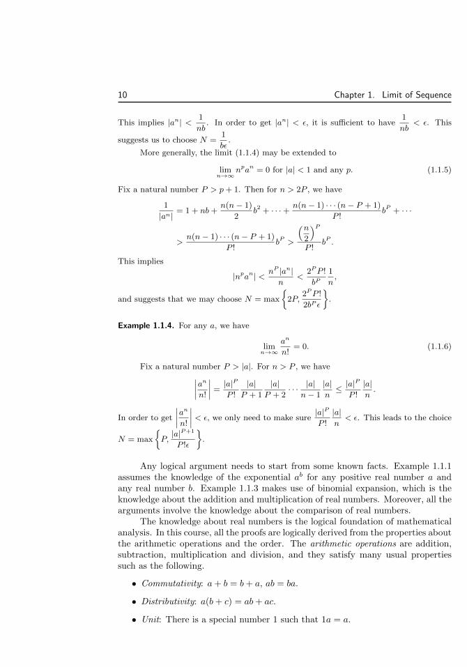
Any logical argument needs to start from some known facts. Example 1.1.1assumes the knowledge of the exponential ab for any positive real number a andany real number b. Example 1.1.3 makes use of binomial expansion, which is theknowledge about the addition and multiplication of real numbers. Moreover, all thearguments involve the knowledge about the comparison of real numbers.
The knowledge about real numbers is the logical foundation of mathematicalanalysis. In this course, all the proofs are logically derived from the properties aboutthe arithmetic operations and the order. The arithmetic operations are addition,subtraction, multiplication and division, and they satisfy many usual propertiessuch as the following.
• Commutativity: a+ b = b+ a, ab = ba.
• Distributivity: a(b+ c) = ab+ ac.
• Unit: There is a special number 1 such that 1a = a.

1.1. Definition 11
An order is a relation a < b defined for all pairs a, b, satisfying the following prop-erties.
• Exclusivity: One and only one from a < b, a = b, b < a can be true.
• Transitivity: a < b and b < c =⇒ a < c.
The arithmetic operations and the order relation should satisfy many compatibilityproperties such as the following.
• (+, <) compatibility: a < b =⇒ a+ c < b+ c.
• (×, <) compatibility: a < b, 0 < c =⇒ ac < bc.
Because of these properties, the real numbers form an ordered field.In fact, the rational numbers also have the arithmetic operations and the order
relation, such that these usual properties are also satisfied. Therefore the rationalnumbers also form an ordered field. The key distinction between the real and therational numbers is the existence of limit. The issue will be discussed in Section 1.4.Due to this extra property, the real numbers form a complete ordered field, whilethe rational numbers form an incomplete ordered field.
A consequence of the existence of the limit is the existence of the exponentialoperation ab for real numbers a > 0 and b. In contrast, within the rational numbers,there is no exponential operation, because ab may be irrational for rational a and b.The exponential of real numbers has many usual properties such as the following.
• Zero: a0 = 1.
• Unit: a1 = a, 1a = 1.
• Addition: ab+c = abac.
• Multiplication: abc = (ab)c, (ab)c = acbc.
• Order: a > b, c > 0 =⇒ ac > bc; and a > 1, b > c =⇒ ab > ac.
The exponential operation and the related properties are not assumptions added tothe real numbers. They can be derived from the existing arithmetic operations andorder relation.
In summary, this course assumes all the knowledge about the arithmetic oper-ations, the exponential operation, and the order relation of real numbers. Startingfrom Definitions 1.4.1 and 1.4.2 in Section 1.4, we will further assume the existenceof limit.
Exercise 1.1. Show that the sequence
1.4, 1.41, 1.414, 1.4142, 1.41421, 1.414213, 1.4142135, 1.41421356, . . .
of more and more refined decimal approximations of√
2 converges to√
2. More generally,a positive real number a > 0 has the decimal expansion
a = X.Z1Z2 · · ·ZnZn+1 · · · ,

12 Chapter 1. Limit of Sequence
where X is a non-negative integer, and Zn is a single digit integer from 0, 1, 2, . . . , 9.Prove that the sequence
X.Z1, X.Z1Z2, X.Z1Z2Z3, X.Z1Z2Z3Z4, . . .
of more and more refined decimal approximations converges to a.
Exercise 1.2. Suppose xn ≤ l ≤ yn and limn→∞(xn − yn) = 0. Prove that limn→∞ xn =limn→∞ yn = l.
Exercise 1.3. Suppose |xn − l| ≤ yn and limn→∞ yn = 0. Prove that limn→∞ xn = l.
Exercise 1.4. Suppose limn→∞ xn = l. Prove that limn→∞ |xn| = |l|. Is the converse true?
Exercise 1.5. Suppose limn→∞ xn = l. Prove that limn→∞ xn+3 = l. Is the converse true?
Exercise 1.6. Prove that the limit is not changed if finitely many terms are modified. Inother words, if there is N , such that xn = yn for n > N , then limn→∞ xn = l if and onlyif limn→∞ yn = l.
Exercise 1.7. Prove the uniqueness of the limit. In other words, if limn→∞ xn = l andlimn→∞ xn = l′, then l = l′.
Exercise 1.8. Prove the following are equivalent to the definition of limn→∞ xn = l.
1. For any c > ε > 0, where c is some fixed number, there is N , such that |xn − l| < εfor all n > N .
2. For any ε > 0, there is a natural number N , such that |xn − l| < ε for all n > N .
3. For any ε > 0, there is N , such that |xn − l| ≤ ε for all n > N .
4. For any ε > 0, there is N , such that |xn − l| < ε for all n ≥ N .
5. For any ε > 0, there is N , such that |xn − l| ≤ 2ε for all n > N .
Exercise 1.9. Which are equivalent to the definition of limn→∞ xn = l?
1. For ε = 0.001, we have N = 1000, such that |xn − l| < ε for all n > N .
2. For any 0.001 ≥ ε > 0, there is N , such that |xn − l| < ε for all n > N .
3. For any ε > 0.001, there is N , such that |xn − l| < ε for all n ≥ N .
4. For any ε > 0, there is a natural number N , such that |xn − l| ≤ ε for all n ≥ N .
5. For any ε > 0, there is N , such that |xn − l| < 2ε2 for all n > N .
6. For any ε > 0, there is N , such that |xn − l| < 2ε2 + 1 for all n > N .
7. For any ε > 0, we have N = 1000, such that |xn − l| < ε for all n > N .
8. For any ε > 0, there are infinitely many n, such that |xn − l| < ε.
9. For infinitely many ε > 0, there is N , such that |xn − l| < ε for all n > N .
10. For any ε > 0, there is N , such that l − 2ε < xn < l + ε for all n > N .
11. For any natural number K, there is N , such that |xn − l| <1
Kfor all n > N .

1.2. Property 13
Exercise 1.10. Write down the complete sets of axioms for the following algebraic struc-tures.
1. Abelian group: A set with addition and subtraction.
2. Field: A set with four arithmetic operations.
3. Ordered field: A set with arithmetic operations and order relation.
1.2 Property
Basic Convergence Property
A sequence is bounded if |xn| ≤ B for some constant B and all n. This is equivalentto B1 ≤ xn ≤ B2 for some constants B1, B2 and all n. The constants B, B1, B2
are respectively called a bound, a lower bound and an upper bound.
Proposition 1.2.1. Convergent sequences are bounded.
Proof. Suppose limn→∞ xn = l. For ε = 1 > 0, there is N , such that
n > N =⇒ |xn − l| < 1 ⇐⇒ l − 1 < xn < l + 1.
Moreover, by taking a bigger natural number if necessary, we may further assumeN is a natural number. Then xN+1, xN+2, . . . , have upper bound l + 1 and lowerbound l − 1, and the whole sequence has upper bound maxx1, x2, . . . , xN , l + 1and lower bound minx1, x2, . . . , xN , l − 1.
Example 1.2.1. The sequences n,√n, 2n, (−3)
√n, (1 + (−1)n)n are not bounded and are
therefore divergent.
Exercise 1.11. Prove that if |xn| < B for n > N , then the whole sequence xn is bounded.This implies that the boundedness is not changed by modifying finitely many terms.
Exercise 1.12. Prove that the addition, subtraction and multiplication of bounded se-quences are bounded. What about the division and exponential operations? What canyou say about the order relation and the boundedness?
Exercise 1.13. Suppose limn→∞ xn = 0 and yn is bounded. Prove that limn→∞ xnyn = 0.
A subsequence of a sequence xn is obtained by selecting some terms. Theindices of the selected terms can be arranged as a strictly increasing sequence n1 <n2 < · · · < nk < · · · , and the subsequence can be denoted as xnk . The followingare two examples of subsequences
x3k : x3, x6, x9, x12, x15, x18, . . . ,
x2k : x2, x4, x8, x16, x32, x64, . . . .
Note that if xn starts from n = 1, then nk ≥ k. Thus by reindexing the terms ifnecessary, we may always assume nk ≥ k in subsequent proofs.

14 Chapter 1. Limit of Sequence
Proposition 1.2.2. Suppose a sequence converges to l. Then all its subsequencesconverge to l.
Proof. Suppose limn→∞ xn = l. For any ε > 0, there is N , such that n > N implies|xn − l| < ε. Then
k > N =⇒ nk ≥ k > N =⇒ |xnk − l| < ε.
Example 1.2.2. The sequence (−1)n has subsequences (−1)2k = 1 and (−1)2k+1 = −1.Since the two subsequences have different limits, the original sequence diverges. This alsogives a counterexample to the converse of Proposition 1.2.1. The right converse of theproposition is given by Theorem 1.5.1.
Exercise 1.14. Explain why the sequences diverge.
1. 3√−n.
2.(−1)n2n+ 1
n+ 2.
3.(−1)n2n(n+ 1)
(√n+ 2)3
.
4.√n(√
n+ (−1)n −√n− (−1)n
).
5.n sin
nπ
3
n cosnπ
2+ 2
.
6. x2n =1
n, x2n+1 = n
√n.
7. x2n = 1, x2n+1 =√n.
8. n√
2n + 3(−1)nn.
Exercise 1.15. Prove that limn→∞ xn = l if and only if limk→∞ x2k = limk→∞ x2k+1 = l.
Exercise 1.16. Suppose xn is the union of two subsequences xmk and xnk . Prove thatlimn→∞ xn = l if and only if limk→∞ xmk = limk→∞ xnk = l. This extends Exercise 1.15.In general, if a sequence xn is the union of finitely many subsequences xni,k , i = 1, . . . , p,k = 1, 2, . . . , then limn→∞ xn = l if and only if limk→∞ xni,k = l for all i.
Arithmetic Property
Proposition 1.2.3 (Arithmetic Rule). Suppose
limn→∞
xn = l, limn→∞
yn = k.
Then
limn→∞
(xn + yn) = l + k, limn→∞
xnyn = lk, limn→∞
xnyn
=l
k,
where yn 6= 0 and k 6= 0 are assumed in the third equality.
Proof. For any ε > 0, there are N1 and N2, such that
n > N1 =⇒ |xn − l| <ε
2,
n > N2 =⇒ |yn − k| <ε
2.

1.2. Property 15
Then for n > maxN1, N2, we have
|(xn + yn)− (l + k)| ≤ |xn − l|+ |yn − k| <ε
2+ε
2= ε.
This completes the proof that limn→∞(xn + yn) = l + k.By Proposition 1.2.1, we have |yn| < B for a fixed number B and all n. For
any ε > 0, there are N1 and N2, such that
n > N1 =⇒ |xn − l| <ε
2B,
n > N2 =⇒ |yn − k| <ε
2|l|.
Then for n > maxN1, N2, we have
|xnyn − lk| = |(xnyn − lyn) + (lyn − lk)|
≤ |xn − l||yn|+ |l||yn − k| <ε
2BB + |l| ε
2|l|= ε.
This completes the proof that limn→∞ xnyn = lk.
Assume yn 6= 0 and k 6= 0. We will prove limn→∞1
yn=
1
k. Then by the
product property of the limit, this implies
limn→∞
xnyn
= limn→∞
xn limn→∞
1
yn= l
1
k=l
k.
For any ε > 0, we have ε′ = min
ε|k|2
2,|k|2
> 0. Then there is N , such that
n > N =⇒ |yn − k| < ε′
⇐⇒ |yn − k| <ε|k|2
2, |yn − k| <
|k|2
=⇒ |yn − k| <ε|k|2
2, |yn| >
|k|2
=⇒∣∣∣∣ 1
yn− 1
k
∣∣∣∣ =|yn − k||ynk|
<
ε|k|2
2|k|2|k|
= ε.
This completes the proof that limn→∞1
yn=
1
k.
Exercise 1.17. Here is another way of proving the limit of the quotient.
1. Prove that |y − 1| < ε <1
2implies
∣∣∣∣1y − 1
∣∣∣∣ < 2ε.
2. Prove that lim yn = 1 implies lim1
yn= 1.

16 Chapter 1. Limit of Sequence
3. Use the the second part and the limit of multiplication to prove the limit of thequotient.
Exercise 1.18. Suppose limn→∞ xn = l and limn→∞ yn = k. Prove that
limn→∞
maxxn, yn = maxl, k, limn→∞
minxn, yn = minl, k.
You may use the formula maxx, y =1
2(x+y+ |x−y|) and the similar one for minx, y.
Exercise 1.19. What is wrong with the following application of Propositions 1.2.2 and 1.2.3:The sequence xn = (−1)n satisfies xn+1 = −xn. Therefore
limn→∞
xn = limn→∞
xn+1 = − limn→∞
xn,
and we get limn→∞ xn = 0.
Order Property
Proposition 1.2.4 (Order Rule). Suppose xn and yn converge.
1. xn ≥ yn for sufficiently big n =⇒ limn→∞ xn ≥ limn→∞ yn.
2. limn→∞ xn > limn→∞ yn =⇒ xn > yn for sufficiently big n.
A special case of the property is that
xn ≥ l for big n =⇒ limn→∞
xn ≥ l,
andlimn→∞
xn > l =⇒ xn > l for big n.
We also have the ≤ and < versions of the special case.
Proof. We prove the second statement first. By Proposition 1.2.3, the assumptionimplies ε = limn→∞(xn − yn) = limn→∞ xn − limn→∞ yn > 0. Then there is N ,such that
n > N =⇒ |(xn − yn)− ε| < ε =⇒ xn − yn − ε > −ε ⇐⇒ xn > yn.
By exchanging xn and yn in the second statement, we find that
limn→∞
xn < limn→∞
yn =⇒ xn < yn for big n.
This further implies that we cannot have xn ≥ yn for big n. The combined impli-cation
limn→∞
xn < limn→∞
yn =⇒ opposite of (xn ≥ yn for big n)
is equivalent to the first statement.

1.2. Property 17
In the second part of the proof above, we used the logical fact that “A =⇒ B”is the same as “(not B) =⇒ (not A)”. Moreover, we note that the following twostatements are not opposite of each other.
• xn < yn for big n: There is N , such that xn < yn for n > N .
• xn ≥ yn for big n: There is N , such that xn ≥ yn for n > N .
In fact, the opposite of the second statement is the following: For any N , there isn > N , such that xn < yn. The first statement implies this opposite statement.But the opposite of the second statement does not imply the first statement.
Proposition 1.2.5 (Sandwich Rule). Suppose
xn ≤ yn ≤ zn, limn→∞
xn = limn→∞
zn = l.
Then limn→∞ yn = l.
Proof. For any ε > 0, there is N , such that
n > N =⇒ |xn − l| < ε, |zn − l| < ε
=⇒ l − ε < xn, zn < l + ε
=⇒ l − ε < xn ≤ yn ≤ zn < l + ε
⇐⇒ |yn − l| < ε.
In the proof above, we usually have N1 and N2 for limn→∞ xn and limn→∞ znrespectively. Then N = maxN1, N2 works for both limits. In the later arguments,we may always choose the same N for finitely many limits.
Example 1.2.3. For any a > 1 and n > a, we have 1 < n√a < n
√n. Thus by the limit
(1.1.3) and the sandwich rule, we have limn→∞ n√a = 1. On the other hand, for 0 < a < 1,
we have b =1
a> 1 and
limn→∞
n√a = lim
n→∞
1n√b
=1
limn→∞n√b
= 1.
Combining all the cases, we get limn→∞ n√a = 1 for any a > 0.
Exercise 1.20. Redo Exercise 1.3 by using the sandwich rule.
Exercise 1.21. Let a > 0 be a constant. Then1
n< a < n for big n. Use this and the limit
(1.1.3) to prove limn→∞ n√a = 1.
Cauchy Criterion
The definition of convergence involves the explicit value of the limit. However,there are many cases that a sequence must be convergent, but the limit value is not

18 Chapter 1. Limit of Sequence
known. The limit of the world record in 100 meter dash is one such example. Insuch cases, the convergence cannot be established by using the definition alone.
On the other hand, we have used Propositions 1.2.1 and 1.2.2 to show thedivergence of some sequences. However, Example 1.2.2 shows that the criterion ofPropositions 1.2.1 is too crude for the convergence. Propositions 1.2.2 is also uselessfor providing a convergence criterion. So a more fundamental theory is needed.
Theorem 1.2.6 (Cauchy1 Criterion). Suppose a sequence xn converges. Then forany ε > 0, there is N , such that
m,n > N =⇒ |xm − xn| < ε.
Proof. Suppose limn→∞ xn = l. For any ε > 0, there is N , such that n > N implies
|xn − l| <ε
2. Then m,n > N implies
|xm − xn| = |(xm − l)− (xn − l)| ≤ |xm − l|+ |xn − l| <ε
2+ε
2= ε.
Cauchy criterion plays a critical role in analysis. Therefore the criterion iscalled a theorem instead of just a proposition. Moreover, a special name is given tothe property in the criterion.
Definition 1.2.7. A sequence xn is called a Cauchy sequence if for any ε > 0, thereis N , such that
m,n > N =⇒ |xm − xn| < ε.
Theorem 1.2.6 says that convergent sequences must be Cauchy sequences. Theconverse will be established in Theorem 1.5.2 and is one of the most fundamentalresults in analysis.
Example 1.2.4. Consider the sequence xn = (−1)n. For ε = 1 > 0 and any N , we canfind an even n > N . Then m = n + 1 > N is odd and |xm − xn| = 2 > ε. Therefore theCauchy criterion fails and the sequence diverges.
Example 1.2.5 (Oresme2). The harmonic sequence
xn = 1 +1
2+
1
3+ · · ·+ 1
n
1Augustin Louis Cauchy, born 1789 in Paris (France), died 1857 in Sceaux (France). His con-tributions to mathematics can be seem by the numerous mathematical terms bearing his name,including Cauchy integral theorem (complex functions), Cauchy-Kovalevskaya theorem (differen-tial equations), Cauchy-Riemann equations, Cauchy sequences. He produced 789 mathematicspapers and his collected works were published in 27 volumes.
2Nicole Oresme, born 1323 in Allemagne (France), died 1382 in Lisieux (France). Oresme isbest known as an economist, mathematician, and a physicist. He was one of the most famous andinfluential philosophers of the later Middle Ages. His contributions to mathematics were mainlycontained in his manuscript Tractatus de configuratione qualitatum et motuum (Treatise on theConfiguration of Qualities and Motions).

1.3. Infinity and Infinitesimal 19
satisfies
x2n − xn =1
n+ 1+
1
n+ 2+ · · ·+ 1
2n≥ 1
2n+
1
2n+ · · ·+ 1
2n=
n
2n=
1
2.
Thus for ε =1
2and any N , we have |xm − xn| >
1
2by taking any natural number n > N
and m = 2n. Therefore the Cauchy criterion fails and the harmonic sequence diverges.
Example 1.2.6. We show that xn = sinn diverges. For any integer k, the intervals(2kπ +
π
4, 2kπ +
3π
4
)and
(2kπ − π
4, 2kπ − 3π
4
)have length
π
2> 1 and therefore must
contain integers mk and nk. Moreover, by taking k to be a big positive number, mk
and nk can be as big as we wish. Then sinmk >1√2
, sinnk < − 1√2
, and we have
| sinmk − sinnk| >√
2. Thus the sequence sinn is not Cauchy and must diverge.For extensions of the example, see Exercises 1.23 and 1.30.
Exercise 1.22. For the harmonic sequence xn, use x2n − xn >1
2to prove that x2n >
n
2.
Then show the divergence of xn.
Exercise 1.23. For 0 < a < π, prove that both sinna and cosna diverge.
Exercise 1.24. Prove any Cauchy sequence is bounded.
Exercise 1.25. Prove that a subsequence of a Cauchy sequence is still a Cauchy sequence.
1.3 Infinity and InfinitesimalA changing numerical quantity is an infinity if it tends to get arbitrarily big. Forsequences, this means the following.
Definition 1.3.1. A sequence xn diverges to infinity, denoted limn→∞ xn = ∞, iffor any b, there is N , such that
n > N =⇒ |xn| > b. (1.3.1)
It diverges to positive infinity, denoted limn→∞ xn = +∞, if for any b, there is N ,such that
n > N =⇒ xn > b.
It diverges to negative infinity, denoted limn→∞ xn = −∞, if for any b, there is N ,such that
n > N =⇒ xn < b.
A changing numerical quantity is an infinitesimal if it tends to get arbitrarilysmall. For sequences, this means that for any ε > 0, there is N , such that
n > N =⇒ |xn| < ε. (1.3.2)

20 Chapter 1. Limit of Sequence
This is the same as limn→∞ xn = 0.Note that the implications (1.3.1) and (1.3.2) are equivalent by changing xn
to1
xnand taking ε =
1
b. Therefore we have
xn is an infinity ⇐⇒ 1
xnis an infinitesimal.
We also note that, since limn→∞ xn = l is equivalent to limn→∞(xn − l) = 0, wehave
xn converges to l ⇐⇒ xn − l is an infinitesimal.
Exercise 1.26. Infinities must be unbounded. Is the converse true?
Exercise 1.27. Prove that if a sequence diverges to infinity, then all its subsequences divergeto infinity.
Exercise 1.28. Suppose limn→∞ xn = limn→∞ yn = +∞. Prove that limn→∞(xn + yn) =+∞ and limn→∞ xnyn = +∞.
Exercise 1.29. Suppose limn→∞ xn =∞ and |xn − xn+1| < c for some constant c.
1. Prove that either limn→∞ xn = +∞ or limn→∞ xn = −∞.
2. If we further know limn→∞ xn = +∞, prove that for any a > x1, some term xn liesin the interval (a, a+ c).
Exercise 1.30. Prove that if limn→∞ xn = +∞ and |xn − xn+1| < c for some constantc < π, then sinxn diverges. Exercise 1.29 might be helpful here.
Some properties of finite limits can be extended to infinities and infinitesimals.For example, the properties in Exercise 1.28 can be denoted as the arithmetic rules(+∞) + (+∞) = +∞ and (+∞)(+∞) = +∞. Moreover, if limn→∞ xn = 1,
limn→∞ yn = 0, and yn < 0 for big n, then limn→∞xnyn
= −∞. Thus we have
another arithmetic rule1
0−= −∞. Common sense suggests more arithmetic rules
such as
c+∞ =∞, c · ∞ =∞ for c 6= 0, ∞ ·∞ =∞,∞c
=∞, c
0=∞ for c 6= 0,
c
∞= 0,
where c is a finite number and represents a sequence converging to c. On the otherhand, we must be careful not to overextend the arithmetic rules. The following
example shows that0
0has no definite value.
limn→∞
n−1 = 0, limn→∞
2n−1 = 0, limn→∞
n−2 = 0,
limn→∞
n−1
2n−1=
1
2, lim
n→∞
n−1
n−2= +∞, lim
n→∞
n−2
2n−1= 0.

1.4. Supremum and Infimum 21
Exercise 1.31. Prove properties of infinity.
1. (bounded)+∞ =∞: If xn is bounded and limn→∞ yn =∞, then limn→∞(xn+yn) =∞.
2. (−∞)(−∞) = +∞.
3. min+∞,+∞ = +∞.
4. Sandwich rule: If xn ≥ yn and limn→∞ yn = +∞, then limn→∞ xn = +∞.
5. (> c > 0) · (+∞) = +∞: If xn > c for some constant c > 0 and limn→∞ yn = +∞,then limn→∞ xnyn = +∞.
Exercise 1.32. Show that∞+∞ has no definite value by constructing examples of sequencesxn and yn that diverge to ∞ but one of the following holds.
1. limn→∞(xn + yn) = 2.
2. limn→∞(xn + yn) = +∞.
3. xn + yn is bounded and divergent.
Exercise 1.33. Show that 0 ·∞ has no definite value by constructing examples of sequencesxn and yn, such that limn→∞ xn = 0 and limn→∞ yn =∞ and one of the following holds.
1. limn→∞ xnyn = 2.
2. limn→∞ xnyn = 0.
3. limn→∞ xnyn =∞.
4. xnyn is bounded and divergent.
Exercise 1.34. Provide counterexamples to the wrong arithmetic rules.
+∞+∞ = 1, (+∞)− (+∞) = 0, 0 · ∞ = 0, 0 · ∞ =∞, 0 · ∞ = 1.
1.4 Supremum and InfimumTo discuss the converse of Theorem 1.2.6, we have to consider the difference betweenrational and real numbers. Specifically, consider the converse of Cauchy criterionstated for the real and the rational number systems:
1. Real number Cauchy sequences always have real number limits.
2. Rational number Cauchy sequences always have rational number limits.
The key distinction here is that, although a sequence of rational numbers may havea limit, the limit may be irrational. For example, the rational number sequence ofthe decimal approximations of
√2 in Exercise 1.1 is a Cauchy sequence but has no
rational number limit. This shows that the second statement is wrong.Therefore the truthfulness of the first statement is closely related to the funda-
mental question of the definition of real numbers. In other words, the establishmentof the first property must also point to the key difference between the rational andthe real number systems. One solution to the fundamental question is to simply

22 Chapter 1. Limit of Sequence
use the converse of Cauchy criterion as the way of constructing real numbers fromrational numbers, by demanding that all Cauchy sequences converge. This is thetopological approach and can be dealt with in the larger context of the completionof metric spaces. Alternatively, real numbers can be constructed by considering theorder among the numbers. The subsequent discussion will be based on this moreintuitive approach, which is called the Dedekind3 cut.
Definition 1.4.1. Let X be a nonempty set of numbers. An upper bound of X is anumber B such that x ≤ B for any x ∈ X. The supremum of X is the least upperbound of the set and is denoted supX.
The existence of the supremum is what distinguishes the real numbers fromthe rational numbers.
Definition 1.4.2. Real numbers is a set with the usual arithmetic operations and theorder satisfying the usual properties, and the additional property that any boundedset of real numbers has the supremum.
Supremum and Infimum
The supremum λ = supX is characterized by the following properties.
1. λ is an upper bound: For any x ∈ X, we have x ≤ λ.
2. Any number smaller than λ is not an upper bound: For any ε > 0, there isx ∈ X, such that x > λ− ε.
The lower bound and the infimum inf X can be similarly defined and characterized.
Example 1.4.1. Both the set 1, 2 and the interval [0, 2] have 2 as the supremum. Ingeneral, the maximum of a set X is a number ξ ∈ X satisfying ξ ≥ x for any x ∈ X. Ifthe maximum exists, then the maximum is the supremum. We also note that the interval(0, 2) has no maximum but still has 2 as the supremum.
A bounded set of real numbers may not always have maximum, but always hassupremum. Similar discussion can be made for the minimum.
Example 1.4.2. The irrational number√
2 is the supremum of the set
1.4, 1.41, 1.414, 1.4142, 1.41421, 1.414213, 1.4142135, 1.41421356, . . .
of its decimal expansions. It is also the supremum of the setmn
: m and n are natural numbers satisfying m2 < 2n2
of positive rational numbers whose squares are less than 2.
3Julius Wilhelm Richard Dedekind, born 1831 and died 1916 in Braunschweig (Germany).Dedekind came up with the idea of the cut on November 24 of 1858 while thinking how to teachcalculus. He made important contributions to algebraic number theory. His work introduced anew style of mathematics that influenced generations of mathematicians.

1.4. Supremum and Infimum 23
Example 1.4.3. Let Ln be the length of an edge of the inscribed regular n-gon in a circleof radius 1. Then 2π is the supremum of the set 3L3, 4L4, 5L5, . . . of the circumferencesof the inscribed regular n-gons.
Exercise 1.35. Find the suprema and the infima.
1. a+ b : a, b are rational, a2 < 3, |2b+ 1| < 5.
2.
n
n+ 1: n is a natural number
.
3.
(−1)nn
n+ 1: n is a natural number
.
4.mn
: m and n are natural numbers satisfying m2 > 3n2
.
5.
1
2m+
1
3n: m and n are natural numbers
.
6. nRn : n ≥ 3 is a natural number, where Rn is the length of an edge of the circum-scribed regular n-gon around a circle of radius 1.
Exercise 1.36. Prove that the supremum is unique.
Exercise 1.37. Suppose X is a nonempty bounded set of numbers. Prove that λ = supXis characterized by the following two properties.
1. λ is an upper bound: For any x ∈ X, we have x ≤ λ.
2. λ is the limit of a sequence in X: There are xn ∈ X, such that λ = limn→∞ xn.
The following are some properties of the supremum and infimum.
Proposition 1.4.3. Suppose X and Y are nonempty bounded sets of numbers.
1. supX ≥ inf X, and the equality holds if and only if X contains a singlenumber.
2. supX ≤ inf Y if and only if x ≤ y for any x ∈ X and y ∈ Y .
3. supX ≥ inf Y if and only if for any ε > 0, there are x ∈ X and y ∈ Ysatisfying y − x < ε.
4. Let X + Y = x+ y : x ∈ X, y ∈ Y . Then sup(X + Y ) = supX + supY andinf(X + Y ) = inf X + inf Y .
5. Let cX = cx : x ∈ X. Then sup(cX) = c supX when c > 0 and sup(cX) =c inf X when c < 0. In particular, sup(−X) = − inf X.
6. Let XY = xy : x ∈ X, y ∈ Y . If all numbers in X,Y are positive, thensup(XY ) = supX supY and inf(XY ) = inf X inf Y .
7. Let X−1 = x−1 : x ∈ X. If all numbers in X are positive, then supX−1 =(inf X)−1.

24 Chapter 1. Limit of Sequence
8. |x − y| ≤ c for any x ∈ X and y ∈ Y if and only if | supX − supY | ≤ c,| inf X − inf Y | ≤ c, | supX − inf Y | ≤ c and | inf X − supY | ≤ c.
Proof. For the first property, we pick any x ∈ X and get supx ≥ x ≥ inf X. Whensupx = inf X, we get x = supx = inf X, so that X contains a single number.
For the second property, supX ≤ inf Y implies x ≤ supX ≤ inf Y ≤ y forany x ∈ X and y ∈ Y . Conversely, assume x ≤ y for any x ∈ X and y ∈ Y . Thenany y ∈ Y is an upper bound of X. Therefore supX ≤ y. Since supX ≤ y for anyy ∈ Y , supX is a lower bound of Y . Therefore supX ≤ inf Y .
For the third property, for any ε > 0, there are x ∈ X satisfying x > supX− ε2
and y ∈ Y satisfying y < inf Y + ε2 . If supX ≥ inf Y , then this implies y − x <
(inf Y + ε2 )−(supX− ε
2 ) = inf Y −supX+ε ≤ ε. Conversely, suppose for any ε > 0,there are x ∈ X and y ∈ Y satisfying y − x < ε. Then supX − inf Y ≥ x− y ≥ −ε.Since ε > 0 is arbitrary, we get supX − inf Y ≥ 0.
For the fourth property, we have x + y ≤ supX + supY for any x ∈ X andy ∈ Y . This means supX + supY is an upper bound of X + Y . Moreover, for anyε > 0, there are x ∈ X and y ∈ Y satisfying x > supX − ε
2 and y > supY − ε2 .
Then x+ y ∈ X + Y satisfies x+ y > supX + supY − ε. Thus the two conditionsfor supX + supY to be the supremum of X + Y are verified.
For the fifth property, assume c > 0. Then l > x for all x ∈ X is the same ascl > cx for all x ∈ X. Therefore l is an upper bound of X if and only if cl is anupper bound of cX. In particular, l is the smallest upper bound of X if and only ifcl is the smallest upper bound of cX. This means sup(cX) = c supX.
On the other hand, assume c < 0. Then l < x for all x ∈ X is the same ascl > cx for all x ∈ X. Therefore l is a lower bound of X if and only if cl is an upperbound of cX. This means sup(cX) = c inf X.
The proof of the last three properties are left to the reader.
Exercise 1.38. Finish the proof of Proposition 1.4.3.
Exercise 1.39. Suppose Xi are nonempty sets of numbers. Let X = ∪iXi and λi = supXi.Prove that supX = supi λi = supi supXi. What about the infimum?
Monotone Sequence
Recall the example of the world record in 100 meter dash. As the time goes by, therecord is shorter and shorter time, and the limit should be the infimum of all theworld records. The example suggests that a bounded (so that the infimum exists)decreasing sequence should converge to its infimum.
A sequence xn is increasing if xn+1 ≥ xn. It is strictly increasing if xn+1 > xn.The concepts of decreasing and strictly decreasing sequences can be similarly defined.A sequence is monotone if it is either increasing or decreasing.
Proposition 1.4.4. Bounded monotone sequences of real numbers converge. Un-bounded monotone sequences of real numbers diverge to infinity.

1.4. Supremum and Infimum 25
Proof. A bounded and increasing sequence xn has a real number supremum l =supxn. For any ε > 0, by the second property that characterizes the supremum,there is N , such that xN > l − ε. Since the sequence is increasing, n > N impliesxn ≥ xN > l − ε. We also have xn ≤ l because l is an upper bound. Thus weconclude that
n > N =⇒ l − ε < xn ≤ l =⇒ |xn − l| < ε.
This proves that the sequence converges to l.If xn is unbounded and increasing, then it has no upper bound (see Exercise
1.40). In other words, for any b, there is N , such that xN > b. Since the sequenceis increasing, we have
n > N =⇒ xn ≥ xN > b.
This proves that the sequence diverges to +∞.The proof for decreasing sequences is similar.
Example 1.4.4. The harmonic sequence in Example 1.2.5 is clearly increasing. Since it isdivergent, the sequence has no upper bound, and Proposition 1.4.4 tells us
limn→∞
(1 +
1
2+
1
3+ · · ·+ 1
n
)= +∞.
On the other hand, the increasing sequence
xn = 1 +1
22+
1
32+ · · ·+ 1
n2
converges because the following shows that the sequence is bounded
xn < 1 +1
1 · 2 +1
2 · 3 + · · ·+ 1
(n− 1)n
= 1 +
(1
1− 1
2
)+
(1
2− 1
3
)+ · · ·+
(1
n− 1− 1
n
)= 1 +
1
1− 1
n< 2.
Example 1.4.5. The natural constant e is defined as the limit
e = limn→∞
(1 +
1
n
)n= 2.71828182845904 · · · . (1.4.1)
Here we justify the definition by showing that the limit converges.
Let xn =
(1 +
1
n
)n. The binomial expansion tells us
xn = 1 + n
(1
n
)+n(n− 1)
2!
(1
n
)2
+n(n− 1)(n− 2)
3!
(1
n
)3
+ · · ·+ n(n− 1) · · · 1n!
(1
n
)n= 1 +
1
1!+
1
2!
(1− 1
n
)+
1
3!
(1− 1
n
)(1− 2
n
)+ · · ·+ 1
n!
(1− 1
n
)(1− 2
n
)· · ·(
1− n− 1
n
).

26 Chapter 1. Limit of Sequence
By comparing the similar formula for xn+1, we find the sequence is strictly increasing.The formula also tells us (see Example 1.4.4)
xn < 1 +1
1!+
1
2!+
1
3!+ · · ·+ 1
n!< 1 + 1 +
1
1 · 2 +1
2 · 3 + · · ·+ 1
(n− 1)n< 3.
Therefore the sequence converges.The inequality above also shows
e = limn→∞
xn ≤ limn→∞
(1 +
1
1!+
1
2!+ · · ·+ 1
n!
).
On the other hand, for fixed k and any n > k, the binomial expansion tells us
xn ≥ 1 +1
1!+
1
2!
(1− 1
n
)+
1
3!
(1− 1
n
)(1− 2
n
)+ · · ·+ 1
k!
(1− 1
n
)(1− 2
n
)· · ·(
1− k − 1
n
).
Taking n→∞ while fixing k, this implies
e = limn→∞
xn ≥ 1 +1
1!+
1
2!+ · · ·+ 1
k!.
Since this holds for any k, we get
e ≥ limk→∞
(1 +
1
1!+
1
2!+ · · ·+ 1
k!
).
Combined with the inequality in the other direction proved earlier, we get
e = limn→∞
(1 +
1
1!+
1
2!+ · · ·+ 1
n!
).
Exercise 1.40. Prove that an increasing sequence is bounded if and only if it has an upperbound.
Exercise 1.41. Prove that limn→∞ an = 0 for |a| < 1 in the following steps.
1. Prove that for 0 ≤ a < 1, the sequence an decreases.
2. Prove that for 0 ≤ a < 1, the limit of an must be 0.
3. Prove that limn→∞ an = 0 for −1 < a ≤ 0.
1.5 Convergent Subsequence
Bolzano-Weierstrass Theorem
Proposition 1.2.1 says any convergent sequence is bounded. The counterexample(−1)n shows that the converse of the proposition is not true. Despite the diver-gence, we still note that the sequence is made up of two convergent subsequences(−1)2k−1 = −1 and (−1)2k = 1.

1.5. Convergent Subsequence 27
Theorem 1.5.1 (Bolzano4-Weierstrass5 Theorem). A bounded sequence of real num-bers has a convergent subsequence.
By Proposition 1.2.2, any subsequence of a convergent sequence is convergent.The theorem says that, if the original sequence is only assumed to be bounded, then“any subsequence” should be changed to “some subsequence”.
Proof. The bounded sequence xn lies in a bounded interval [a, b]. Divide [a, b] into
two equal halves
[a,a+ b
2
]and
[a+ b
2, b
]. Then one of the halves must contain
infinitely many xn. We denote this interval by [a1, b1].
Further divide [a1, b1] into two equal halves
[a1,
a1 + b12
]and
[a1 + b1
2, b1
].
Again one of the halves, which we denote by [a2, b2], contains infinitely many xn.Keep going, we get a sequence of intervals
[a, b] ⊃ [a1, b1] ⊃ [a2, b2] ⊃ · · · ⊃ [ak, bk] ⊃ · · ·
with the length bk − ak =b− a
2k. Moreover, each internal [ak, bk] contains infinitely
many xn.The inclusion relation between the intervals implies
a ≤ a1 ≤ a2 ≤ · · · ≤ ak ≤ · · · ≤ bk ≤ · · · ≤ b2 ≤ b1 ≤ b.
Since ak and bk are also bounded, by Proposition 1.4.4, both sequences converge.Moreover, by Example 1.1.3, we have
limk→∞
(bk − ak) = (b− a) limk→∞
1
2k= 0.
Therefore ak and bk converge to the same limit l.Since [a1, b1] contains infinitely many xn, we have xn1 ∈ [a1, b1] for some
n1. Since [a2, b2] contains infinitely many xn, we also have xn2∈ [a2, b2] for some
n2 > n1. Keep going, we have a subsequence satisfying xnk ∈ [ak, bk]. This meansthat ak ≤ xnk ≤ bk. By the sandwich rule, we get limk→∞ xnk = l. Thus xnk is aconverging subsequence.
The following useful remark is used in the proof above. Suppose P is a propertyabout terms in a sequence (say xn > l, or xn > xn+1, or xn ∈ [a, b], for examples).Then the following statements are equivalent.
4Bernard Placidus Johann Nepomuk Bolzano, born October 5, 1781, died December 18, 1848in Prague, Bohemia (now Czech). Bolzano is famous for his 1837 book “Theory of Science”.He insisted that many results which were thought ”obvious” required rigorous proof and madefundamental contributions to the foundation of mathematics. He understood the need to redefineand enrich the concept of number itself and define the Cauchy sequence four years before Cauchy’swork appeared.
5Karl Theodor Wilhelm Weierstrass, born October 31, 1815 in Ostenfelde, Westphalia (nowGermany), died February 19, 1848 in Berlin, Germany. In 1864, he found a continuous but nowheredifferentiable function. His lectures on analytic functions, elliptic functions, abelian functionsand calculus of variations influenced many generations of mathematicians, and his approach stilldominates the teaching of analysis today.

28 Chapter 1. Limit of Sequence
1. There are infinitely many xn with property P .
2. For any N , there is n > N , such that xn has property P .
3. There is a subsequence xnk , such that each term xnk has property P .
Example 1.5.1. In Example 1.2.6, we showed that the sequence sinn diverges. On theother hand, Bolzano-Weierstrass theorem tells us that some subsequence sinnk converges.
In fact, any number in [−1, 1] is the limit of some converging subsequence of sinn.Here we show that 0 is the limit of some converging subsequence. The Hurwitz Theoremin number theory says that, for any irrational number such as π, there are infinitely many
rational numbersn
m, m,n ∈ Z, such that
∣∣∣ nm− π
∣∣∣ ≤ 1√5m2
. The constant√
5 can be
changed to a bigger one for π, but is otherwise optimal if π is replaced by the golden ratio√5 + 1
2.
The existence of infinitely many rational approximations as above gives us strictly
increasing sequences mk, nk of natural numbers, such that
∣∣∣∣ nkmk− π
∣∣∣∣ ≤ 1√5m2
k
. This
implies |nk −mkπ| ≤1
mkand limk→∞(nk −mkπ) = 0. Then the continuity of sinx at 0
(see Section 2.2) implies limk→∞ sinnk = limk→∞ sin(nk −mkπ) = 0.Exercise 1.81 gives a vast generalization of the example.
Exercise 1.42. Explain that any real number is the limit of a sequence of the formn1
10,n2
100,
n3
1000, . . . , where nk are integers. Based on this observation, construct a sequence such
that any real number in [0, 1] is the limit of a convergent subsequence.
Exercise 1.43. Prove that a number is the limit of a convergent subsequence of xn if andonly if it is the limit of a convergent subsequence of n
√nxn.
Exercise 1.44. Suppose xn and yn are two bounded sequences. Prove that there are nk,such that both subsequences xnk and ynk converge. Moreover, extend this to more thantwo bounded sequences.
Cauchy Criterion
Now we are ready to prove the converse of Theorem 1.2.6.
Theorem 1.5.2. Any Cauchy sequence of real numbers converges.
Proof. Let xn be a Cauchy sequence. We first prove that the sequence is bounded.For ε = 1 > 0, there is N , such that m,n > N implies |xm − xn| < 1. Takingm = N + 1, we find n > N implies xN+1 − 1 < xn < xN+1 + 1. Thereforemaxx1, x2, . . . , xN , xN+1 + 1 and minx1, x2, . . . , xN , xN+1 − 1 are upper andlower bounds for the sequence.
By Bolzano-Weierstrass Theorem, there is a subsequence xnk converging to a

1.5. Convergent Subsequence 29
limit l. Thus for any ε > 0, there is K, such that
k > K =⇒ |xnk − l| <ε
2.
On the other hand, since xn is a Cauchy sequence, there is N , such that
m,n > N =⇒ |xm − xn| <ε
2.
Now for any n > N , we can easily find some k > K, such that nk > N (k =
maxK,N+1, for example). Then we have both |xnk− l| <ε
2and |xnk−xn| <
ε
2.
The inequalities imply |xn − l| < ε, so we established the implication
n > N =⇒ |xn − l| < ε.
The proof can be summarised in three steps.
1. A Cauchy sequence is bounded.
2. Bounded sequence has converging subsequence.
3. If a Cauchy sequence has a convergent subsequence, then the whole Cauchysequence converges.
We note that the first and third steps are general facts in any metric space, andthe Bolzano-Weierstrass Theorem is only used in the second step. Therefore theequivalence between Cauchy property and convergence remains true in any generalsetting as long as Bolzano-Weierstrass Theorem remains true.
Set of Limits
By Bolzano-Weierstrass Theorem, for a bounded sequence xn, the set LIMxn ofall the limits of convergent subsequences is not empty. The numbers in LIMxnare characterized below.
Proposition 1.5.3. A real number l is the limit of a convergent subsequence of xnif and only if for any ε > 0, there are infinitely many xn satisfying |xn − l| < ε.
We remark that the criterion means that, for any ε > 0 and N , there is n > N ,such that |xn − l| < ε.
Proof. Suppose l = limk→∞ xnk . For any ε > 0, there is K, such that k > Kimplies |xnk − l| < ε. Then xnk for all k > K are the infinitely many xn satisfying|xn − l| < ε.
Conversely, suppose for any ε > 0, there are infinitely many xn satisfying|xn − l| < ε. Then for ε = 1, there is n1 satisfying |xn1
− l| < 1. Next, for
ε =1
2, there are infinitely many xn satisfying |xn − l| < 1
2. Among these we
can find n2 > n1, such that |xn2 − l| <1
2. After finding xnk , we have infinitely

30 Chapter 1. Limit of Sequence
many xn satisfying |xn − l| <1
k + 1. Among these we can find nk+1 > nk, such
that |xnk+1− l| < 1
k + 1. We inductively constructed a subsequence xnk satisfying
|xnk − l| <1
k. The inequality implies limk→∞ xnk = l.
Example 1.5.2. Let xn, yn, zn be sequences converging to l1, l2, l3, respectively. Then theset LIM of limits of the sequence
x1, y1, z1, x2, y2, z2, x3, y3, z3, . . . , xn, yn, zn, . . .
contains l1, l2, l3. We claim that LIM = l1, l2, l3.We need to explain that any l 6= l1, l2, l3 is not the limit of any subsequence. Pick
an ε > 0 satisfying
|l − l1| ≥ 2ε, |l − l2| ≥ 2ε, |l − l3| ≥ 2ε.
Then there is N , such that
n > N =⇒ |xn − l1| < ε, |yn − l2| < ε, |zn − l3| < ε.
Since |l − l1| ≥ 2ε and |xn − l1| < ε imply |xn − l| > ε, we have
n > N =⇒ |xn − l| > ε, |yn − l| > ε, |zn − l| > ε.
This implies that l cannot be the limit of any convergent subsequence.A more direct argument is the following. Let l be the limit of a convergent subse-
quence wm of the combined sequence. The subsequence wm must contain infinitely manyterms from at least one of the three sequences. If wm contains infinitely many terms fromxn, then it contains a subsequence xnk , and we get
l = limwm = limxnk = limxn = l1.
Here Proposition 1.2.2 is applied to the second and the third equalities.
Exercise 1.45. For sequences in Exercise 1.14, find the sets of limits.
Exercise 1.46. Suppose the sequence zn is obtained by combining two sequences xn and yntogether. Prove that LIMzn = LIMxn ∪ LIMyn.
Exercise 1.47. Suppose lk ∈ LIMxn and limk→∞ lk = l. Prove that l ∈ LIMxn. Inother words, the limit of limits is a limit.
Upper and Lower Limits
The supremum of LIMxn is called the upper limit and denoted limn→∞ xn. Theinfimum of LIMxn is called the lower limit and denoted limn→∞ xn. For example,for the sequence in Example 1.5.2, the upper limit is maxl1, l2, l3 and the lowerlimit is minl1, l2, l3.
The following characterizes the upper limit. The lower limit can be similarlycharacterized.
1.5. Convergent Subsequence 31
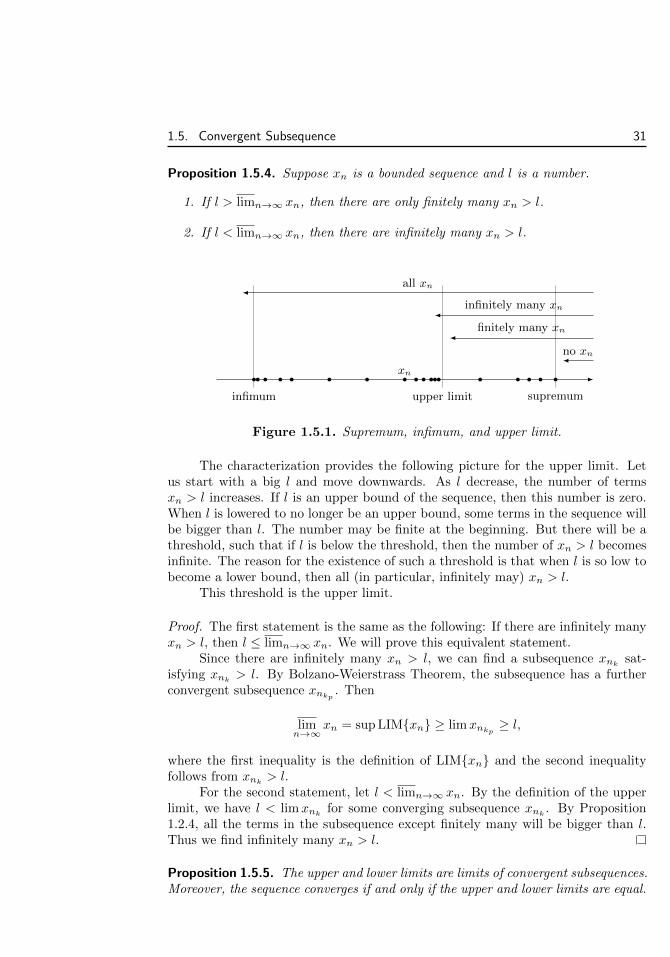
Proposition 1.5.4. Suppose xn is a bounded sequence and l is a number.
1. If l > limn→∞ xn, then there are only finitely many xn > l.
2. If l < limn→∞ xn, then there are infinitely many xn > l.
infimum upper limit supremum
xn
no xn
finitely many xn
infinitely many xn
all xn
Figure 1.5.1. Supremum, infimum, and upper limit.
The characterization provides the following picture for the upper limit. Letus start with a big l and move downwards. As l decrease, the number of termsxn > l increases. If l is an upper bound of the sequence, then this number is zero.When l is lowered to no longer be an upper bound, some terms in the sequence willbe bigger than l. The number may be finite at the beginning. But there will be athreshold, such that if l is below the threshold, then the number of xn > l becomesinfinite. The reason for the existence of such a threshold is that when l is so low tobecome a lower bound, then all (in particular, infinitely may) xn > l.
This threshold is the upper limit.
Proof. The first statement is the same as the following: If there are infinitely manyxn > l, then l ≤ limn→∞ xn. We will prove this equivalent statement.
Since there are infinitely many xn > l, we can find a subsequence xnk sat-isfying xnk > l. By Bolzano-Weierstrass Theorem, the subsequence has a furtherconvergent subsequence xnkp . Then
limn→∞
xn = sup LIMxn ≥ limxnkp ≥ l,
where the first inequality is the definition of LIMxn and the second inequalityfollows from xnk > l.
For the second statement, let l < limn→∞ xn. By the definition of the upperlimit, we have l < limxnk for some converging subsequence xnk . By Proposition1.2.4, all the terms in the subsequence except finitely many will be bigger than l.Thus we find infinitely many xn > l.
Proposition 1.5.5. The upper and lower limits are limits of convergent subsequences.Moreover, the sequence converges if and only if the upper and lower limits are equal.

32 Chapter 1. Limit of Sequence
The first conclusion is limn→∞ xn, limn→∞ xn ∈ LIMxn. In the secondconclusion, the equality limn→∞ xn = limn→∞ xn = l means LIMxn = l, whichbasically says that all convergent subsequences have the same limit.
Proof. Denote l = limxn. For any ε > 0, we have l+ ε > limxn and l− ε < limxn.By Proposition 1.5.4, there are only finitely many xn > l + ε and infinitely manyxn > l−ε. Therefore there are infinitely many xn satisfying l+ε ≥ xn > l−ε. Thusfor any ε > 0, there are infinitely many xn satisfying |xn − l| ≤ ε. By Proposition1.5.3, l is the limit of a convergent subsequence.
For the second part, Proposition 1.2.2 says that if xn converges to l, thenLIMxn = l, so that limxn = limxn = l. Conversely, suppose limxn = limxn =l. Then for any ε > 0, we apply Proposition 1.5.4 to l + ε > limxn and find onlyfinitely many xn > l + ε. We also apply the similar characterization of the lowerlimit to l− ε < limxn and find also only finitely many xn < l− ε. Thus |xn− l| ≤ εholds for all but finitely many xn. If N is the biggest index for those xn that donot satisfy |xn − l| ≤ ε, then we get |xn − l| ≤ ε for all n > N . This proves that xnconverges to l.
Exercise 1.48. Find the upper and lower limits of bounded sequences in Exercise 1.14.
Exercise 1.49. Prove the properties of upper and lower limits.
1. limn→∞(−xn) = − limn→∞ xn.
2. limn→∞ xn + limn→∞ yn ≥ limn→∞(xn + yn) ≥ limn→∞ xn + limn→∞ yn.
3. If xn > 0, then limn→∞1
xn=
1
limn→∞ xn.
4. If xn ≥ 0 and yn ≥ 0, then limn→∞ xn · limn→∞ yn ≥ limn→∞(xnyn) ≥ limn→∞ xn ·limn→∞ yn.
5. If xn ≥ yn, then limn→∞ xn ≥ limn→∞ yn and limn→∞ xn ≥ limn→∞ yn.
6. If limn→∞ xn > limn→∞ yn or limn→∞ xn > limn→∞ yn, then xn > yn for infinitelymany n.
7. If for any N , there are m,n > N , such that xm ≥ yn, then limxn ≥ lim yn.
8. If limxn > lim yn, then for any N , there are m,n > N , such that xm > yn.
Exercise 1.50. Suppose the sequence zn is obtained by combining two sequences xn and yntogether. Prove that lim zn = maxlimxn, lim yn.
Exercise 1.51. Prove that if limn→∞
∣∣∣∣xn+1
xn
∣∣∣∣ < 1, then limn→∞ xn = 0. Prove that if
limn→∞
∣∣∣∣xn+1
xn
∣∣∣∣ > 1, then limn→∞ xn =∞.
Exercise 1.52. Prove that the upper limit l of a bounded sequence xn is characterized bythe following two properties.
1. l is the limit of a convergent subsequence.
2. For any ε > 0, there is N , such that xn < l + ε for any n > N .

1.5. Convergent Subsequence 33
The characterization may be compared with the one for the supremum in Exercise 1.37.
Exercise 1.53. Here is an alternative proof of Theorem 1.5.2 on the convergence of Cauchysequences. Let xn be a Cauchy sequence.
1. Prove that for any ε > 0 and converging subsequences xmk and xnk , we have |xmk −xnk | ≤ ε for sufficiently large k.
2. Prove that for any ε > 0 and l, l′ ∈ LIMxn, we have |l − l′| ≤ ε.
3. Prove that LIMxn consists of a single number.
By Proposition 1.5.5, the last result implies that the sequence converges.
Exercise 1.54. For a bounded sequence xn, prove that
limn→∞
xn = limn→∞
supxn, xn+1, xn+2, . . . ,
limn→∞
xn = limn→∞
infxn, xn+1, xn+2, . . . .
Heine-Borel Theorem
The Bolzano-Weierstrass Theorem has a set theoretical version that plays a crucialrole in the point set topology. The property will not be needed for the analysis ofsingle variable functions but will be useful for multivariable functions. The otherreason for including the result here is that the proof is very similar to the proof ofBolzano-Weierstrass Theorem.
A set X of numbers is closed if xn ∈ X and limn→∞ xn = l implies l ∈ X.Intuitively, this means that one cannot escape X by taking limits. For example,the order rule (Proposition 1.2.4) says that closed intervals [a, b] are closed sets. Inmodern topological language, the following theorem says that bounded and closedsets of numbers are compact.
Theorem 1.5.6 (Heine6-Borel7 Theorem). Suppose X is a bounded and closed set ofnumbers. Suppose (ai, bi) is a collection of open intervals such that X ⊂ ∪(ai, bi).Then X ⊂ (ai1 , bi1) ∪ (ai2 , bi2) ∪ · · · ∪ (ain , bin) for finitely many intervals in thecollection.
We say U = (ai, bi) is an open cover of X when X ⊂ ∪(ai, bi). The theoremsays that if X is bounded and closed, then any cover of X by open intervals has afinite subcover.
Proof. The bounded set X is contained in a bounded and closed interval [α, β].Suppose X cannot be covered by finitely many open intervals in U = (ai, bi).
6Heinrich Eduard Heine, born March 15, 1821 in Berlin, Germany, died October 21, 1881 inHalle, Germany. In addition to the Heine-Borel theorem, Heine introduced the idea of uniformcontinuity.
7Felix Edouard Justin Emile Borel, born January 7, 1871 in Saint-Affrique, France, died Febru-ary 3, 1956 in Paris France. Borel’s measure theory was the beginning of the modern theory offunctions of a real variable. He was French Minister of the Navy from 1925 to 1940.

34 Chapter 1. Limit of Sequence
Similar to the proof of Bolzano-Weierstrass Theorem, we divide [α, β] into two
halves I ′ =
[α,α+ β
2
]and I ′′ =
[α+ β
2, β
]. Then either X ∩ I ′ or X ∩ I ′′ cannot
be covered by finitely many open intervals in U . We denote the correspondinginterval by I1 = [α1, β1] and denote X1 = X ∩ I1.
Further divide I1 into I ′1 =
[α1,
α1 + β1
2
]and I ′′1 =
[α1 + β1
2, β1
]. Again
either X1 ∩ I ′1 or X1 ∩ I ′′1 cannot be covered by finitely many open intervals in U .We denote the corresponding interval by I2 = [α2, β2] and denote X2 = X ∩ I2.Keep going, we get a sequence of intervals
I = [α, β] ⊃ I1 = [α1, β1] ⊃ I2 = [α2, β2] ⊃ · · · ⊃ In = [αn, βn] ⊃ · · ·
with In having length βn−αn =β − α
2n. Moreover, Xn = X ∩ In cannot be covered
by finitely many open intervals in U . This implies that Xn is not empty, so that wecan pick xn ∈ Xn.
As argued in the proof of Bolzano-Weierstrass Theorem, we have converginglimit l = limn→∞ αn = limn→∞ βn. By αn ≤ xn ≤ βn and the sandwich rule, weget l = limn→∞ xn. Then by the assumption that X is closed, we get l ∈ X.
Since X ⊂ ∪(ai, bi), we have l ∈ (ai0 , bi0) for some interval (ai0 , bi0) ∈ U .Then by l = limn→∞ αn = limn→∞ βn, we have Xn ⊂ In = [αn, βn] ⊂ (ai0 , bi0) forsufficiently big n. In particular, Xn can be covered by one open interval in U . Thecontradiction shows that X must be covered by finitely many open intervals fromU .
Exercise 1.55. Find a collection U = (ai, bi) that covers (0, 1], but (0, 1] cannot be coveredby finitely many intervals in U . Find similar counterexample for [0,+∞) in place of (0, 1].
Exercise 1.56 (Lebesgue8). Suppose [α, β] is covered by a collection U = (ai, bi). Denote
X = x ∈ [α, β] : [α, x] is covered by finitely many intervals in U.
1. Prove that supX ∈ X.
2. Prove that if x ∈ X and x < β, then x+ δ ∈ X for some δ > 0.
3. Prove that supX = β.
This proves Heine-Borel Theorem for bounded and closed intervals.
Exercise 1.57. Prove Heine-Borel Theorem for a bounded and closed set X in the followingway. Suppose X is covered by a collection U = (ai, bi).
1. Prove that there is δ > 0, such that for any x ∈ X, (x− δ, x+ δ) ⊂ (ai, bi) for some(ai, bi) ∈ U .
8Henri Leon Lebesgue, born 1875 in Beauvais (France), died 1941 in Paris (France). His 1901paper “Sur une generalisation de l’integrale definie” introduced the concept of measure and revo-lutionized the integral calculus. He also made major contributions in other areas of mathematics,including topology, potential theory, the Dirichlet problem, the calculus of variations, set theory,the theory of surface area and dimension theory.

1.6. Additional Exercise 35
2. Use the boundedness of X to find finitely many numbers c1, c2, . . . , cn, such thatX ⊂ (c1, c1 + δ) ∪ (c2, c2 + δ) ∪ · · · ∪ (cn, cn + δ).
3. Prove that if X ∩ (cj , cj + δ) 6= ∅, then (cj , cj + δ) ⊂ (ai, bi) for some (ai, bi) ∈ U .
4. Prove that X is covered by no more than n open intervals in U .
1.6 Additional ExerciseRatio Rule
Exercise 1.58. Suppose
∣∣∣∣xn+1
xn
∣∣∣∣ ≤ ∣∣∣∣yn+1
yn
∣∣∣∣.1. Prove that |xn| ≤ c|yn| for some constant c.
2. Prove that limn→∞ yn = 0 implies limn→∞ xn = 0.
3. Prove that limn→∞ xn =∞ implies limn→∞ yn =∞.
Note that in order to get the limit, the comparison only needs to hold for sufficiently bign.
Exercise 1.59. Suppose limn→∞xn+1
xn= l. What can you say about limn→∞ xn by looking
at the value of l?
Exercise 1.60. Use the ratio rule to get (1.1.5) and limn→∞(n!)2an
(2n)!.
Power Rule
The power rule says that if limn→∞ xn = l > 0, then limn→∞ xpn = lp. This is a special
case of the exponential rule in Exercises 2.23 and 2.24.
Exercise 1.61. For integer p, show that the power rule is a special case of the arithmeticrule.
Exercise 1.62. Suppose xn ≥ 1 and limn→∞ xn = 1. Use the sandwich rule to prove thatlimn→∞ x
pn = 1 for any p. Moreover, show that the same is true if xn ≤ 1.
Exercise 1.63. Suppose limn→∞ xn = 1. Use minxn, 1 ≤ xn ≤ maxxn, 1, Exercise 1.18and the sandwich rule to prove that limn→∞ x
pn = 1.
Exercise 1.64. Prove the power rule in general.
Average Rule
For a sequence xn, the average sequence is yn =x1 + x2 + · · ·+ xn
n.
Exercise 1.65. Prove that if |xn − l| < ε for n > N , where N is a natural number, then
n > N =⇒ |yn − l| <|x1|+ |x2|+ · · ·+ |xN |+N |l|
n+ ε.

36 Chapter 1. Limit of Sequence
Exercise 1.66. Prove that if limn→∞ xn = l, then limn→∞ yn = l.
Exercise 1.67. If limn→∞ xn =∞, can you conclude limn→∞ yn =∞? What about +∞?
Exercise 1.68. Find suitable condition on a sequence an of positive numbers, such that
limn→∞ xn = l implies limn→∞a1x1 + a2x2 + · · ·+ anxn
a1 + a2 + · · ·+ an= l.
Extended Supremum and Extended Upper Limit
Exercise 1.69. Extend the number system by including the “infinite numbers” +∞, −∞and introduce the order −∞ < x < +∞ for any real number x. Then for any nonemptyset X of real numbers and possibly +∞ or −∞, we have supX and inf X similarly defined.Prove that there are exactly three possibilities for supX.
1. If X has no finite number upper bound or +∞ ∈ X, then supX = +∞.
2. If X has a finite number upper bound and contains at least one finite real number,then supX is a finite real number.
3. If X = −∞, then supX = −∞.
Write down the similar statements for inf X.
Exercise 1.70. For a not necessarily bounded sequence xn, extend the definition of LIMxnby adding +∞ if there is a subsequence diverging to +∞, and adding −∞ if there is asubsequence diverging to −∞. Define the upper and lower limits as the supremum andinfimum of LIMxn, using the extension of the concepts in Exercise 1.69. Prove thefollowing extensions of Proposition 1.5.5.
1. A sequence with no upper bound must have a subsequence diverging to +∞. Thismeans limn→∞ xn = +∞.
2. If there is no subsequence with finite limit and no subsequence diverging to −∞,then the whole sequence diverges to +∞.
Supremum and Infimum in Ordered Set
Recall that an order on a set is a relation x < y between pairs of elements satisfying thetransitivity and the exclusivity. The concepts of upper bound, lower bound, supremumand infimum can be defined for subsets of an ordered set in a way similar to numbers.
Exercise 1.71. Provide a characterization of the supremum similar to numbers.
Exercise 1.72. Prove that the supremum, if exists, must be unique.
Exercise 1.73. An order is defined for all subsets of the plane R2 by A ≤ B if A is containedin B. Let R be the set of all rectangles centered at the origin and with circumference 1.Find the supremum and infimum of R.
The Limits of the Sequence sinn
In Example 1.5.1, we used a theorem from number theory to prove that a subsequenceof sinn converges to 0. Here is a more general approach that proves that any number in[−1, 1] is the limit of a converging subsequence of sinn.

1.6. Additional Exercise 37
The points on the unit circle S1 are described by the angles θ. Note that the samepoint also corresponds to θ + 2mπ for integers m. Now for any angle α, the rotation byangle α is the map Rα : S1 → S1 that takes the angle θ to θ+ α. If we apply the rotationn times, we get Rnα = Rnα : S1 → S1 that takes the angle θ to θ + nα. The rotation alsohas inverse R−1
α = R−α : S1 → S1 that takes the angle θ to θ − α.An interval (θ1, θ2) on the circle S1 consists of all points corresponding to angles
θ1 < θ < θ2. The interval may be also described as (θ1 + 2mπ, θ2 + 2mπ) and has lengthθ2− θ1. A key property of the rotation is the preservation of angle length. In other words,the length of Rα(θ1, θ2) = (θ1 + α, θ2 + α) is the same as the length of (θ1, θ2).
We fix an angle θ and also use θ to denote the corresponding point on the circle. Wealso fix a rotation angle α and consider all the points
X = Rnα(θ) = θ + nα : n ∈ Z
obtained by rotating θ by angle α repeatedly.
Exercise 1.74. Prove that if an interval (θ1, θ2) on the circle S1 does not contain points inX, then for any n, Rnα(θ1, θ2) does not contain points in X.
Exercise 1.75. Suppose (θ1, θ2) is a maximal open interval that does not contain points inX. In other words, any bigger open interval will contain some points in X. Prove that forany n, either Rnα(θ1, θ2) is disjoint from (θ1, θ2) or Rnα(θ1, θ2) = (θ1, θ2).
Exercise 1.76. Suppose there is an open interval containing no points in X. Prove thatthere is a maximal open interval (θ1, θ2) containing no points in X. Moreover, we haveRnα(θ1, θ2) = (θ1, θ2) for some natural number n.
Exercise 1.77. Prove that Rnα(θ1, θ2) = (θ1, θ2) for some natural number n if and only if αis a rational multiple of π.
Exercise 1.78. Prove that if α is not a rational multiple of π, then every open intervalcontains some point in X.
Exercise 1.79. Prove that if every open interval contains some point in X, then for anyangle l, there is a sequence nk of integers that diverge to infinity, such that the sequenceRnkα (θ) = θ + nkα on the circle converges to l. Then interpret the result as limk→∞ |θ +
nkα− 2mkπ| = 0 for another sequence of integers mk.
Exercise 1.80. Prove that if α is not a rational multiple of π, then there are sequences ofnatural numbers mk, nk diverging to +∞, such that limk→∞ |nkα− 2mkπ| = 0. Then usethe result to improve the nk in Exercise 1.79 to be natural numbers.
Exercise 1.81. Suppose θ is any number and α is not a rational multiple of π. Prove thatany number in [−1, 1] is the limit of a converging subsequence of sin(θ + nα).
Alternative Proof of Bolzano-Weierstrass Theorem
We say a term xn in a sequence has property P if there is M , such that m > M impliesxm > xn. The property means that xm > xn for sufficiently big m.

38 Chapter 1. Limit of Sequence
Exercise 1.82. Suppose there are infinitely many terms in a sequence xn with property P .Construct an increasing subsequence xnk in which each xnk has property P . Moreover, incase xn is bounded, prove that xnk converges to limxn.
Exercise 1.83. Suppose there are only finitely many terms in a sequence xn with propertyP . Construct a decreasing subsequence xnk .
Set Version of Bolzano-Weierstrass Theorem, Upper Limit and Lower Limit
Let X be a set of numbers. A number l is a limit of X if for any ε > 0, there is x ∈ Xsatisfying 0 < |x − l| < ε. The definition is similar to the characterisation of the limit ofa subsequence in Proposition 1.5.3. Therefore the limit of a set is the analogue of limit ofconverging subsequences. We may similarly denote all the limits of the set by LIMX (thecommon notation in topology is X ′, called derived set).
Exercise 1.84. Prove that l is a limit of X if and only if l is the limit of a non repetitive(i.e., no two terms are equal) sequence in X. This is the analogue of Proposition 1.5.3.
Exercise 1.85. What does it mean for a number not to be a limit? Explain that a finite sethas no limit.
Exercise 1.86. Prove the set version of Bolzano-Weierstrass Theorem: Any infinite, boundedand closed set of numbers has an accumulation point. Here we say X is closed if limxn = land xn ∈ X imply l ∈ X.
Exercise 1.87. Use the set version of Bolzano-Weierstrass Theorem to prove Theorem 1.5.1,the sequence version.
Exercise 1.88. Use LIMX to define the upper limit limX and the lower limit limX of aset. Then establish the analogue of Proposition 1.5.4 that characterises the two limits.
Exercise 1.89. Prove that limX and limX are also limits of X. Moreover, explain whathappens when limX = limX. The problem is the analogue of Proposition 1.5.5.
Exercise 1.90. Try to extend Exercises 1.49, 1.50, 1.54 to infinite and bounded sets ofnumbers.

Chapter 2
Limit of Function
39

40 Chapter 2. Limit of Function
2.1 DefinitionFor a function f(x) defined near a (but not necessarily at a), we may consider itsbehavior as x approaches a.
Definition 2.1.1. A function f(x) defined near a has limit l at a, and denotedlimx→a f(x) = l, if for any ε > 0, there is δ > 0, such that
0 < |x− a| < δ =⇒ |f(x)− l| < ε. (2.1.1)
δδ
ε
εl
a
Figure 2.1.1. 0 < |x− a| < δ implies |f(x)− l| < ε.
The definition says
x→ a, x 6= a =⇒ f(x)→ l.
Similar to the sequence limit, the smallness ε for |f(x)− l| is arbitrarily given, whilethe size δ for |x − a| is to be found after ε is given. Thus the choice of δ usuallydepends on ε and is often expressed as a function of ε. Moreover, since the limit isabout how close the numbers are, only small ε and δ need to be considered.
Variations of Function Limit
In the definition of function limit, x may approach a from the right (i.e., x > a) orfrom the left (i.e., x < a). The two approaches may be treated separately, leadingto one sided limits.
Definition 2.1.2. A function f(x) defined for x > a and near a has right limit l ata, and denoted limx→a+ f(x) = l, if for any ε > 0, there is δ > 0, such that
0 < x− a < δ =⇒ |f(x)− l| < ε. (2.1.2)
A function f(x) defined for x < a and near a has left limit l at a, and denotedlimx→a− f(x) = l, if for any ε > 0, there is δ > 0, such that
−δ < x− a < 0 =⇒ |f(x)− l| < ε. (2.1.3)

2.1. Definition 41
The one sided limits are often denoted as f(a+) = limx→a+ f(x) and f(a−) =limx→a− f(x). Moreover, the one sided limits and the usual (two sided) limit arerelated as follows.
Proposition 2.1.3. limx→a f(x) = l if and only if limx→a+ f(x) = limx→a− f(x) =l.
Proof. The two sided limit implies the two one sided limits, because (2.1.1) implies(2.1.2) and (2.1.3). Conversely, if limx→a+ f(x) = limx→a− f(x) = l, then for anyε > 0, there are δ+, δ− > 0, such that
0 < x− a < δ+ =⇒ |f(x)− l| < ε,
−δ− < x− a < 0 =⇒ |f(x)− l| < ε.
Then for 0 < |x − a| < δ = minδ+, δ−, we have either 0 < x − a < δ ≤ δ+ or−δ− ≤ −δ < x− a < 0. In either case, we get |f(x)− l| < ε.
We may also define the function limit when x gets very big.
Definition 2.1.4. A function f(x) has limit l at∞, denoted limx→∞ f(x) = l, if forany ε > 0, there is N , such that
|x| > N =⇒ |f(x)− l| < ε.
The limit at infinity can also be split into the limits f(+∞) = limx→+∞ f(x),f(−∞) = limx→−∞ f(x) at positive and negative infinities. Proposition 2.1.3 alsoholds for the limit at infinity.
The divergence to infinity can also be defined for functions.
Definition 2.1.5. A function f(x) diverges to infinity at a, denoted limx→a f(x) =∞, if for any b, there is δ > 0, such that
0 < |x− a| < δ =⇒ |f(x)| > b.
The divergence to positive and negative infinities, denoted limx→a f(x) =+∞ and limx→a f(x) = −∞ respectively, can be similarly defined. Moreover, thedivergence to infinity at the left of a, the right of a, or when a is various kinds ofinfinities, can also be similarly defined.
Similar to sequences, we know limx→a f(x) =∞ if and only if limx→a1
f(x)=
0, i.e., the reciprocal is an infinitesimal.
Exercise 2.1. Write down the rigorous definition of limx→+∞ f(x) = l, limx→a+ f(x) =−∞, limx→∞ f(x) = +∞.
Exercise 2.2. Suppose f(x) ≤ l ≤ g(x) and limx→a(f(x)−g(x)) = 0. Prove that limx→a f(x) =limx→a g(x) = l. Extend Exercises 1.3 through 1.7 in similar way.

42 Chapter 2. Limit of Function
Exercise 2.3. Prove the following are equivalent definitions of limx→a f(x) = l.
1. For any ε > 0, there is δ > 0, such that 0 < |x− a| ≤ δ implies |f(x)− l| < ε.
2. For any c > ε > 0, where c is some fixed number, there is δ > 0, such that 0 <|x− a| < δ implies |f(x)− l| ≤ ε.
3. For any natural number n, there is δ > 0, such that 0 < |x − a| < δ implies
|f(x)− l| ≤ 1
n.
4. For any 1 > ε > 0, there is δ > 0, such that 0 < |x−a| < δ implies |f(x)−l| < ε
1− ε .
Exercise 2.4. Which are equivalent to the definition of limx→a f(x) = l?
1. For ε = 0.001, we have δ = 0.01, such that 0 < |x− a| ≤ δ implies |f(x)− l| < ε.
2. For any ε > 0, there is δ > 0, such that |x− a| < δ implies |f(x)− l| < ε.
3. For any ε > 0, there is δ > 0, such that 0 < |x− a| < δ implies 0 < |f(x)− l| < ε.
4. For any 0.001 ≥ ε > 0, there is δ > 0, such that 0 < |x−a| ≤ 2δ implies |f(x)−l| ≤ ε.
5. For any ε > 0.001, there is δ > 0, such that 0 < |x− a| ≤ 2δ implies |f(x)− l| ≤ ε.
6. For any ε > 0, there is a rational number δ > 0, such that 0 < |x − a| < δ implies|f(x)− l| < ε.
7. For any ε > 0, there is a natural number N , such that 0 < |x − a| < 1
Nimplies
|f(x)− l| < ε.
8. For any ε > 0, there is δ > 0, such that 0 < |x− a| < δ implies |f(x)− l| < ε2.
9. For any ε > 0, there is δ > 0, such that 0 < |x− a| < δ implies |f(x)− l| < ε2 + 1.
10. For any ε > 0, there is δ > 0, such that 0 < |x− a| < δ + 1 implies |f(x)− l| < ε2.
Basic Properties of the Function Limit
The properties of limit of sequences can be extended to functions.
Proposition 2.1.6. The limit of functions has the following properties.
1. Boundedness: A function convergent at a is bounded near a.
2. Arithmetic: Suppose limx→a f(x) = l and limx→a g(x) = k. Then
limx→a
(f(x) + g(x)) = l + k, limx→a
f(x)g(x) = lk, limx→a
f(x)
g(x)=l
k,
where g(x) 6= 0 and k 6= 0 are assumed in the third equality.
3. Order: Suppose limx→a f(x) = l and limx→a g(x) = k. If f(x) ≥ g(x) for xnear a, then l ≥ k. Conversely, if l > k, then f(x) > g(x) for x near a.
4. Sandwich: Suppose f(x) ≤ g(x) ≤ h(x) for x near a and limx→a f(x) =limx→a h(x) = l. Then limx→a g(x) = l.

2.1. Definition 43
5. Composition: Suppose limx→a f(x) = b, limy→b g(y) = c. If f(x) 6= b for xnear a, or g(b) = c, then limy→a g(f(x)) = c.
When we say something happens near a, we mean that there is δ > 0, suchthat it happens for x satisfying 0 < |x− a| < δ. For example, f(x) is bounded neara if there is δ > 0 and B, such that 0 < |x− a| < δ implies |f(x)| < B.
For a composition
x 7→ y = f(x) 7→ z = g(y) = g(f(x)),
the composition rule says
limx→a
y = b, limy→b
z = c =⇒ limx→a
z = c.
The left side means two implications
x→ a, x 6= a =⇒ y → b,
y → b, y 6= b =⇒ z → c.
However, to combine the two implications to get what we want
x→ a, x 6= a =⇒ z → c,
the right side of the first implication needs to match the left side of the secondimplication. To make the match, we need to either modify the first implication to
x→ a, x 6= a =⇒ y → b, y 6= b,
which is the first additional condition in the fifth statement of Proposition 2.1.6, ormodify the second implication to
y → b =⇒ z → c,
which is the second additional condition.
Proof. The first four properties are parallel to the Propositions 1.2.1 through 1.2.5for the sequence limit, and can be proved in the similar way.
Now we turn to the composition rule. For any ε > 0, by limy→b g(y) = c, thereis µ > 0, such that
0 < |y − b| < µ =⇒ |g(y)− c| < ε. (2.1.4)
For this µ > 0, by limx→a f(x) = b, there is δ > 0, such that
0 < |x− a| < δ =⇒ |f(x)− b| < µ. (2.1.5)
If the additional condition f(x) 6= b for x near a is satisfied, then (2.1.5)becomes
0 < |x− a| < δ =⇒ 0 < |f(x)− b| < µ.

44 Chapter 2. Limit of Function
Combining this with (2.1.4) and taking y = f(x), we get
0 < |x− a| < δ =⇒ 1 < |f(x)− b| < µ =⇒ |g(f(x))− c| < ε.
If the additional condition g(b) = c is satisfied, then (2.1.4) becomes
|y − b| < µ =⇒ |g(y)− c| < ε.
Combining this with (2.1.5) and taking y = f(x), we get
0 < |x− a| < δ =⇒ |f(x)− b| < µ =⇒ |g(f(x))− c| < ε.
So under either additional condition, we proved limy→a g(f(x)) = c.
Proposition 2.1.6 was stated for the two sided limit limx→a f(x) = l with finitea and l only. The properties also hold when a is replaced by a+, a−, ∞, +∞ and−∞.
What about the case that l is infinity? In general, all the valid arithmetic rulesfor sequences that involve infinities and infinitesimals, such as (+∞)+(+∞) = +∞,are still valid for functions. However, as in the sequence case, the same care needsto be taken in applying the arithmetic rules to infinities and infinitesimals.
For the sandwich rule, we have f(x) ≥ g(x) and limx→a g(x) = +∞ implyinglimx→a f(x) = +∞. There is similar sandwich rule for l = −∞ but no sandwichrule for l =∞.
For the composition rule, a, b, c can be practically any symbols. For example,if limx→∞ g(x) = b, g(x) > b and limy→b+ f(y) = c, then limx→∞ f(g(x)) = c.
Example 2.1.1. The limit of power functions will be established in Section 2.2. Sup-pose we know limx→0 x
2 = 0 and limx→0+
√x = 0. We will argue that limx→0 f(x2) =
limx→0+ f(x).If limx→0 f(x2) = l converges, then consider the composition
x 7→ y =√x 7→ z = f(y2) = f(x).
By limx→0+
√x = 0, limx→0 f(x2) = l, and the fact that x > 0 =⇒
√x > 0 (so the first
additional condition is satisfied), we may apply the composition rule to get limx→0+ f(x) =l.
Conversely, if limx→0+ f(x) = l converges, then consider the composition
x 7→ y = x2 7→ z = f(y) = f(x2).
By limx→0 x2 = 0, limx→0+ f(x) = l, and the fact that x 6= 0 =⇒ x2 > 0, we may apply
the composition rule to get limx→0 f(x2) = l.
Exercise 2.5. Prove the first four properties of Proposition 2.1.6.
Exercise 2.6. Assume that we already know the limit of power functions. Rewrite the limitsas limx→a f(x) for suitable a and explain whether the limits are equivalent.

2.1. Definition 45
1. limx→a− f(−x).
2. limx→a+ f(x+ 1).
3. limx→a+ f(bx+ c).
4. limx→0+ f(x2).
5. limx→0 f((x+ 1)3).
6. limx→0+ f(√x).
7. limx→0 f
(1
x
).
8. limx→2+ f
(1
x
).
Exercise 2.7. Prove properties of the function limit.
1. If limx→a f(x) = l and limx→a g(x) = k, then limx→a maxf(x), g(x) = maxl, kand limx→a minf(x), g(x) = minl, k.
2. If limx→a+ f(x) =∞ and there are c > 0 and δ > 0, such that 0 < x−a < δ impliesg(x) > c, then limx→a+ f(x)g(x) =∞.
3. If limx→a g(x) = +∞ and limy→+∞ f(y) = c, then limx→a f(g(x)) = c.
4. If f(x) ≤ g(x) and limx→+∞ g(x) = −∞, then limx→+∞ f(x) = −∞.
Function Limit and Sequence Limit
A sequence can be considered as a function n 7→ xn. The composition of a functionf(x) with a sequence
n 7→ x = xn 7→ y = f(x) = f(xn)
is the restriction of the function to the sequence.
Proposition 2.1.7. Suppose f(x) is a function defined near a. Then limx→a f(x) =l if and only if limn→∞ f(xn) = l for any sequence xn satisfying xn 6= a andlimn→∞ xn = a.
Proof. We prove the case a and l are finite. The other cases are similar.Suppose limx→a f(x) = l. Suppose xn 6= a and limn→∞ xn = a. For any
ε > 0, we can find δ > 0, such that
0 < |x− a| < δ =⇒ |f(x)− l| < ε.
Then we can find N , such that
n > N =⇒ |xn − a| < δ.
The assumption xn 6= a further implies
n > N =⇒ 0 < |xn − a| < δ.
Combining the two implications together, we have
n > N =⇒ 0 < |xn − a| < δ =⇒ |f(xn)− l| < ε.
This proves limn→∞ f(xn) = l.Conversely, assume limx→a f(x) 6= l (which means either the limit does not
exist, or the limit exists but is not equal to l). Then there is ε > 0, such that for any

46 Chapter 2. Limit of Function
δ > 0, there is x satisfying 0 < |x−a| < δ and |f(x)−l| ≥ ε. Specifically, by choosing
δ =1
nfor natural numbers n, we find a sequence xn satisfying 0 < |xn − a| <
1
nand |f(xn) − l| ≥ ε. The first inequality implies xn 6= a and limn→∞ xn = a. Thesecond inequality implies limn→∞ f(xn) 6= l. This proves the converse.
We remark that a subsequence can be considered as the composition of twosequences
k 7→ n = nk 7→ x = xnk .
The Proposition 1.2.2 about the convergence of subsequences can also be consideredas a version of the composition rule.
Example 2.1.2. The Dirichlet9 function is
D(x) =
1, if x is rational,
0, if x is irrational.
For any a, we can find a sequence xn of rational numbers and a sequence yn of irrational
numbers converging to but not equal to a (for a = 0, take xn =1
nand yn =
√2
n, for
example). Then f(xn) = 1 and f(yn) = 0, so that limn→∞ f(xn) = 1 and limn→∞ f(yn) =0. This implies that the Dirichlet function diverges everywhere.
Exercise 2.8. Prove that limx→∞ f(x) = +∞ if and only if limn→∞ f(xn) = +∞ for anysequence xn satisfying limn→∞ xn =∞.
Exercise 2.9. Prove that limx→a f(x) converges if and only if limn→∞ f(xn) converges forany sequence xn satisfying xn 6= a and limn→∞ xn = a.
Exercise 2.10. Prove that limx→a+ f(x) = l if and only if limn→∞ f(xn) = l for anystrictly decreasing sequence xn converging to a. Moreover, state the similar criterionfor limx→+∞ f(x) = l.
More Properties of the Function Limit
A function is increasing if
x > y =⇒ f(x) ≥ f(y).
It is strictly increasing if
x > y =⇒ f(x) > f(y).
The concepts of decreasing and strictly decreasing functions can be similarly defined.A function is monotone if it is either increasing or decreasing.
9Johann Peter Gustav Lejeune Dirichlet, born 1805 in Duren (French Empire, now Germany),died in Gottingen (Germany). He proved the famous Fermat’s Last Theorem for the case n = 5in 1825. He made fundamental contributions to the analytic number theory, partial differentialequation, and Fourier series. He introduced his famous function in 1829.

2.1. Definition 47
Proposition 1.4.4 can be extended to the one sided limit and the limit at signedinfinities of monotone functions. The following is stated for the right limit, and canbe proved in similar way. See Exercises 2.11 and 2.12.
Proposition 2.1.8. Suppose f(x) is a monotone bounded function defined for x > aand x near a. Then limx→a+ f(x) converges.
We also have the Cauchy criterion for the function limit. The following isstated for the usual limit limx→a f(x).
Theorem 2.1.9 (Cauchy Criterion). The limit limx→a f(x) converges if and only iffor any ε > 0, there is δ > 0, such that
0 < |x− a| < δ, 0 < |y − a| < δ =⇒ |f(x)− f(y)| < ε. (2.1.6)
Proof. For the convergence of limx→a f(x) implying the Cauchy criterion, the proofof Theorem 1.2.6 can be adopted without much change.
Conversely, assume f(x) satisfies the Cauchy criterion. Choose a sequencesatisfying xn 6= a and limn→∞ xn = a. We prove that f(xn) is a Cauchy sequence.For any ε > 0, we find δ > 0 such that (2.1.6) holds. Then for this δ > 0, there isN , such that
n > N =⇒ |xn − a| < δ.
The assumption xn 6= a also implies |xn − a| > 0. Combined with (2.1.6), we get
m,n > N =⇒ 0 < |xm − a| < δ, 0 < |xn − a| < δ
=⇒ |f(xm)− f(xn)| < ε.
By Theorem 1.5.2, the sequence f(xn) converges to a limit l.Next we prove that l = limn→∞ f(xn) is also the limit of the function at a.
For any ε > 0, we find δ > 0 such that (2.1.6) holds. Then we find one xn satisfying0 < |xn− a| < δ and |f(xn)− l| < ε. Moreover, for any x satisfying 0 < |x− a| < δ,we may apply (2.1.6) to x and xn to get |f(x)− f(xn)| < ε. Therefore
|f(x)− l| ≤ |f(xn)− l|+ |f(x)− f(xn)| < 2ε.
This completes the proof that limx→a f(x) = l.
Exercise 2.11. Suppose f(x) is increasing on (a, b].
1. If f(x) is bounded, prove that limx→a+ f(x) converges to inf(a,b] f(x).
2. If f(x) is unbounded, prove that limx→a+ f(x) = −∞.
Exercise 2.12. State the similar version of Exercise 2.11 for limx→+∞ f(x).
Exercise 2.13. State and prove the Cauchy criterion for the convergence of limx→a+ f(x)and limx→+∞ f(x).
48 Chapter 2. Limit of Function
Exercise 2.14. Suppose for any ε > 0, there is δ > 0, such that
a− δ < x < a < y < a+ δ =⇒ |f(x)− f(y)| < ε.
Prove that limx→a f(x) converges.
2.2 Basic LimitThis section is devoted to rigorously deriving the important and basic functionlimits.
Polynomial and Rational Function
It is easy to see that limx→a c = c for a constant c and limx→a x = a. Then byrepeatedly applying the arithmetic rule, we get the limit of a polynomial
limx→a
(cnxn + cn−1x
n−1 + · · ·+ c1x+ c0) = cnan + cn−1a
n−1 + · · ·+ c1a+ c0.
Note that the limit is simply the value of the polynomial at a. More generally, arational function
r(x) =cnx
n + cn−1xn−1 + · · ·+ c1x+ c0
dmxm + dm−1xm−1 + · · ·+ d1x+ d0
is a quotient of two polynomials. By the limit of polynomial and the arithmeticrule, we get
limx→a
r(x) =cna
n + cn−1an−1 + · · ·+ c1a+ c0
dmam + dm−1am−1 + · · ·+ d1a+ d0= r(a),
as long as the denominator is nonzero.
We also have limx→∞ c = c and limx→∞1
x= 0. Then by the arithmetic rule,
we get
limx→∞
2x5 + 10
−3x+ 1= limx→∞
x42 + 10
1
x
−3 +1
x
= (+∞)2 + 10 · 0−3 + 0
= −∞,
limx→∞
x3 − 2x2 + 1
−x3 + 1= limx→∞
1− 21
x+
1
x3
−1 +1
x3
=2− 2 · 0 + 03
−1 + 0= −2.
In general, we have the limit
limx→∞
cnxn + cn−1x
n−1 + · · ·+ c1x+ c0dmxm + dm−1xm−1 + · · ·+ d1x+ d0
=
0, if m > n, dm 6= 0,cndm
, if m = n, dm 6= 0,
∞, if m < n, cn 6= 0.
It is also possible to find more refined information on whether the limit is +∞ or−∞. The detail is left to the reader.

2.2. Basic Limit 49
Power Function
The power function xp is defined for x > 0 and any p in general. The function canbe extended to other cases. For example, the function is defined for all x 6= 0 if p isan integer. The function is also defined at 0 if p ≥ 0.
If the exponent p is an integer, then the power function is a special case ofthe rational function, for which we already know the limit. In particular, we havelimx→a x
p = ap in case p is an integer.
1 2 3 4
x1/3
x1/2
x2/3
x
x3/2x2x3
x−3
x−2
x−3/2
x−1
x−2/3
x−1/2
x−1/3
Figure 2.2.1. Power function.
Now for any p, fix a natural number P > |p|. Then for x > 1, we havex−P < xp < xP . By limx→1 x
−P = 1−P = 1, limx→1 xP = 1P = 1, and the
sandwich rule, we get limx→1+ xp = 1. Note that the limit is taken from the rightbecause the sandwich inequality holds for x > 1 only. Similarly, by the inequalityx−P > xp > xP for 0 < x < 1 and the sandwich rule, we get limx→1− x
p = 1.Combining the limits on two sides, we get limx→1 x
p = 1.For the limit of the power function at any a > 0, we move the location of the
limit from a to 1limx→a
xp = limx→1
(ax)p = ap limx→1
xp = ap. (2.2.1)
In the first equality, the composition rule is used for
x 7→ y = ax 7→ z = yp = (ax)p.
We have limx→1 ax = a and x 6= 1 ⇐⇒ y 6= a, so that the first additionalcondition is satisfied. In the second equality, we used the compatibility property(ay)p = apyp between the multiplication and the exponential, and the arithmeticrule for the limit.
The limit (2.2.1) shows that, like rational functions, the limit of a powerfunction is the value of the function.
Now we discuss the limits at 0+ and +∞. If p > 0, then for any ε > 0, wehave
0 < x < δ = ε1p =⇒ 0 < xp < δp = ε.

50 Chapter 2. Limit of Function
This shows that limx→0+ xp = 0, which can be considered as an extension of Ex-ample 1.1.1. The case p < 0 can then be obtained by the arithmetic rule
limx→0+
xp = limx→0+
1
x−p=
1
limx→0+ x−p=
1
0+= +∞ for p < 0.
Combining with x0 = 1 for all x, we get
limx→0+
xp =
0, if p > 0,
1, if p = 0,
+∞, if p < 0.
By substituting the variable x with1
x, we get
limx→+∞
xp =
0, if p < 0,
1, if p = 0,
+∞, if p > 0.
Note that a substitution of variable is exactly the composition. Thereforecomputing the limit by substitution makes use of the composition rule. For example,the substituting above means introducing the composition
x 7→ y =1
x7→ z = y−p =
1
x−p= xp.
We already know the limit limy→0+ y−p of the second function. For the first func-tion, we know x→ +∞ =⇒ y → 0, y > 0. A modified version of the compositionrule can then be applied.
Exercise 2.15. Prove that if limn→∞ xn = l > 0, then limn→∞ xpn = lp. What if l = 0+?
What if l = +∞?
Exercise 2.16. Prove that if limx→a f(x) = l > 0, then limx→a f(x)p = lp. What if l = 0+?What if l = +∞?
Exponential Function
The exponential function cx is defined for c > 0 and all x.Example 1.2.3 tells us limn→∞ c
1n = 1. This suggests that limx→0+ cx = 1.
For the case c ≥ 1, we prove this by comparing with the known sequence limit.
For 0 < x < 1, we have x <1
nfor some natural number n. If c ≥ 1, then
1 ≤ cx ≤ c 1n .
Since c1n converges to 1, it appears that we can conclude the limit of cx by the
sandwich rule. However, we cannot directly cite our existing sandwich rules because

2.2. Basic Limit 51
1x
−4 −3 −2 −1 1 2 3 4
4x ex 2x 1.5x4−xe−x2−x1.5−x
Figure 2.2.2. Exponential function.
they do not compare sequences with functions. Instead, we need to repeat the proofof the sandwich rule.
By limn→∞ c1n = 1, for any ε > 0, there is N , such that n > N implies
|c 1n − 1| < ε. Then
0 < x < δ =1
N + 1=⇒ 0 < x <
1
nfor some natural number n > N
=⇒ 1 ≤ cx ≤ c 1n (because c ≥ 1)
=⇒ |cx − 1| ≤ |c 1n − 1| < ε.
This completes the proof of limx→0+ cx = 1 in case c ≥ 1.
For the case 0 < c ≤ 1, we have1
c≥ 1, and the arithmetic rule gives us
limx→0+
cx =1
limx→0+
(1
c
)x = 1.
Further by substituting x with −x (so the composition rule is used), we have
limx→0−
cx = limx→0+
c−x =1
limx→0+ cx= 1.
This completes the proof that limx→0 cx = 1 for all c > 0.
What about the limit at any a? Like (2.2.1), we may move the location of thelimit from a to 0, where we already know the limit
limx→a
cx = limx→0
ca+x = ca limx→0
cx = ca.
Again, the limit of the exponential function is the same as the value of the function.For the limits at ±∞, Example 1.1.3 says limn→∞ cn = 0 for |c| < 1, which
suggests limx→+∞ cx = 0 for 0 < c < 1. Again this can be established by the spirit

52 Chapter 2. Limit of Function
of the sandwich rule. For any ε > 0, by limn→∞ cn = 0, there is N , such that n > Nimplies |cn| < ε. Then
x > N + 1 =⇒ x > n for some natural number n > N
=⇒ 0 < cx < cn
=⇒ |cx| < |cn| < ε.
By further applying the arithmetic rule and substitution of variable (compositionrule used), we get
limx→+∞
cx =
0, if 0 < c < 1,
1, if c = 1,
+∞, if c > 1,
(2.2.2)
and
limx→−∞
cx =
0, if c > 1,
1, if c = 1,
+∞, if 0 < c < 1.
(2.2.3)
The details are left to readers.
Exercise 2.17. Use the limit (1.1.5) to prove
limx→+∞
xpcx = 0 for 0 < c < 1.
Then discuss all cases for limx→+∞ xpcx.
Exercise 2.18. Use Example 1.2.3 to prove
limx→0+
xx = 1,
Then prove that limx→0+ |p(x)|x = 1 for any nonzero polynomial p(x).
Exercise 2.19. For any c > 0, we have x < c <1
xfor sufficiently small x > 0. Use this to
derive limx→0 cx = 1 from Exercise 2.18.
Exercise 2.20. Prove that if limn→∞ xn = l and c > 0, then limn→∞ cxn = cl. What if
l = +∞? What if l = −∞?
Exercise 2.21. Prove that if limx→a f(x) = l and c > 0, then limx→a cf(x) = cl.
Exercise 2.22. Prove that if 0 < A ≤ f(x) ≤ B and limx→a g(x) = 0, then limx→a f(x)g(x) =1.
Exercise 2.23. Prove the exponential rule: If limx→a f(x) = l > 0 and limx→a g(x) = k,then limx→a f(x)g(x) = lk.
Exercise 2.24. State and prove the exponential rule for sequences.

2.2. Basic Limit 53
Natural Constant e
Another basic limit is the extension of the natural constant in Example 1.4.5
limx→∞
(1 +
1
x
)x= e. (2.2.4)
Logically, we must derive the limit from the definition (1.4.1), which is the onlything we currently know about e.
For x > 1, we have n ≤ x ≤ n+ 1 for some natural number n. This implies(1 +
1
n+ 1
)n≤(
1 +1
x
)x≤(
1 +1
n
)n+1
. (2.2.5)
From the definition of e, we know
limn→∞
(1 +
1
n
)n+1
= limn→∞
(1 +
1
n
)nlimn→∞
(1 +
1
n
)= e,
limn→∞
(1 +
1
n+ 1
)n=
limn→∞
(1 +
1
n+ 1
)n+1
limn→∞
(1 +
1
n+ 1
) = e.
Therefore for any ε > 0, there is N > 0, such that
n > N =⇒
∣∣∣∣∣(
1 +1
n
)n+1
− e
∣∣∣∣∣ < ε,
∣∣∣∣(1 +1
n+ 1
)n− e∣∣∣∣ < ε, (2.2.6)
Then for x > N + 1, we have n ≤ x ≤ n + 1 for some natural number n > N . Bythe inequalities (2.2.5) and (2.2.6), this further implies
−ε <(
1 +1
n+ 1
)n− e ≤
(1 +
1
x
)x− e ≤
(1 +
1
n
)n+1
− e < ε.
This proves limx→+∞
(1 +
1
x
)x= e. By substituting x with −x, we further get
limx→−∞
(1 +
1
x
)x= limx→+∞
(1− 1
x
)−x= limx→+∞
(1 +
1
x− 1
)x−1(1 +
1
x− 1
)= e.
This completes the proof of (2.2.4). Note that substituting x with1
xgives us
limx→0
(1 + x)1x = e. (2.2.7)

54 Chapter 2. Limit of Function
Trigonometric Function
The sine and tangent functions are defined in Figure 2.2.3, at least for 0 ≤ x ≤ π
2.
We have
Area(triangle OBP ) < Area(fan OBP ) < Area(triangle OBQ).
This means
1
2sinx <
1
2x <
1
2tanx for 0 < x <
π
2.
This gives us
0 < sinx < x for 0 < x <π
2, (2.2.8)
and
cosx <sinx
x< 1 for 0 < x <
π
2. (2.2.9)
1
x
O A
sinx
P
B
tanx
Q
Figure 2.2.3. trigonometric function
Applying the sandwich rule to (2.2.8), we get limx→0+ sinx = 0. By substi-tuting x with −x, we get limx→0− sinx = lim−x→0− sin(−x) = − limx→0+ sinx = 0.This proves
limx→0
sinx = 0.
By the arithmetic rule and substituting x withx
2, we get
limx→0
cosx = limx→0
(1− 2 sin2 x
2
)= 1− 2
(limx→0
sinx
2
)2
= 1.
2.3. Continuity 55
Then by trigonometric identities, we have
limx→a
sinx = limx→0
sin(a+ x) = limx→0
(sin a cosx+ cos a sinx)
= sin a · 1 + cos a · 0 = sin a,
limx→a
cosx = limx→0
cos(a+ x) = limx→0
(cos a cosx+ sin a sinx)
= cos a · 1 + sin a · 0 = cos a,
limx→a
tanx =limx→a sinx
limx→a cosx=
sin a
cos a= tan a.
The limits of trigonometric functions are always the values of the functions.Applying limx→0 cosx = 1 and the sandwich rule to (2.2.9), we get
limx→0
sinx
x= 1. (2.2.10)
This further implies
limx→0
tanx
x=
limx→0sinx
xlimx→0 cosx
= 1, (2.2.11)
limx→0
1− cosx
x2= limx→0
2 sin2 x
2x2
= limx→0
2 sin2 x
(2x)2=
1
2
(limx→0
sinx
x
)2
=1
2. (2.2.12)
2.3 ContinuityChanging quantities are often described by functions. Most changes in the realworld are smooth, gradual and well behaved. For example, people do not oftenpress the brake when driving a car, and the climate does not suddenly change fromsummer to winter. The functions describing such well behaved changes are at leastcontinuous.
A function is continuous if its graph “does not break”. The graph of a functionf(x) may break at a for various reasons. But the breaks are always one of the twotypes: Either limx→a f(x) diverges or the limit converges but the limit value is notf(a).
In Figure 2.3.1, the function is continuous at a2, a5 and is not continuousat the other five points. Specifically, limx→a1 f(x) and limx→a7 f(x) diverge be-cause the left and right limits are not equal, limx→a3 f(x) converges but not tof(a1), limx→a4 f(x) diverges because the function is not bounded near a4, andlimx→a6 f(x) diverges because the left limit diverges.
Definition 2.3.1. A function f(x) defined near and include a is continuous at a iflimx→a f(x) = f(a).
Using the ε-δ language, the continuity of f(x) at a means that for any ε > 0,there is δ > 0, such that
|x− a| < δ =⇒ |f(x)− f(a)| < ε. (2.3.1)

56 Chapter 2. Limit of Function
a1 a2 a3 a4 a5 a6 a7
Figure 2.3.1. Continuity and discontinuity.
A function is right continuous at a if limx→a+ f(x) = f(a), and is left con-tinuous if limx→a− f(x) = f(a). For example, the function in Figure 2.3.1 is leftcontinuous at a1 and right continuous at a6, although it is not continuous at thetwo points. A function is continuous at a if and only if it is both left and rightcontinuous at a.
A function defined on an open interval (a, b) is continuous if it is continuousat every point on the interval. A function defined on a closed interval [a, b] iscontinuous if it is continuous at every point on (a, b), is right continuous at a, andis left continuous at b. Continuity for functions on other kinds of intervals can besimilarly defined.
Most basic functions are continuous. Section 2.2 shows that polynomials,rational functions, trigonometric functions, power functions, and exponential func-tions are continuous (at the places where the functions are defined). Then thearithmetic rule and the composition rule further imply the following.
Proposition 2.3.2. The arithmetic combinations and the compositions of continuousfunctions are still continuous.
So functions such as sin2 x + tanx2,x√x+ 1
, 2x costanx
x2 + 1are continuous.
Examples of discontinuity can only be found among more exotic functions.Proposition 2.1.7 implies the following criterion for the continuity in terms of
sequences.
Proposition 2.3.3. A function f(x) is continuous at a if and only if limn→∞ f(xn) =f(a) for any sequence xn converging to a.
The conclusion of the proposition can be written as
limn→∞
f(xn) = f(
limn→∞
xn
). (2.3.2)
On the other hand, the condition g(b) = c in the composition rule in Proposition

2.3. Continuity 57
2.1.6 simply means that g(y) is continuous at b. If we exchange the notations f andg, then the composition rule says that the continuity of f implies
limy→b
f(g(y)) = c = f(b) = f
(limy→b
g(y)
). (2.3.3)
Therefore the function and the limit can be interchanged if the function is contin-uous.
Example 2.3.1. The sign function
sign(x) =
1, if x > 0,
0, if x = 0,
−1, if x < 0,
is continuous everywhere except at 0. The Dirichlet function in Example 2.1.2 is notcontinuous everywhere. Multiplying x to the Dirichlet function produces a function
xD(x) =
x, if x is rational,
0, if x is irrational,
that is continuous only at 0.
sign(x)
irrational
rational
D(x)
irrational
ration
al
xD(x)
Figure 2.3.2. Discontinuous functions.
Example 2.3.2 (Thomae10). For a rational number x =p
q, where p is an integer, q is a
natural number, and p, q are coprime, define R(x) =1
q. For an irrational number x, define
R(x) = 0. Finally define R(0) = 1. We will show that R(x) is continuous at precisely allthe irrational numbers.
Let a be a rational number. Then R(a) 6= 0. On the other hand, we can findirrational numbers xn converging to a. Then limn→∞R(xn) = 0 6= R(a). By Proposition2.3.3, the function is not continuous at a.
10Karl Johannes Thomae, born 1840 in Laucha (Germany), died 1921 in Jena (Germany).Thomae made important contributions to the function theory. In 1870 he showed the conti-nuity in each variable does not imply the joint continuity. He constructed the example here in1875.

58 Chapter 2. Limit of Function
1
1/2
1/31/4
1/51/6
y
x0 irrational 1
Figure 2.3.3. Thomae’s function.
Let a be an irrational number. By the way R(x) is defined, for any natural numberN ,
the numbers x satisfying R(x) ≥ 1
Nare those rational numbers
p
qwith q ≤ N . Therefore
on any bounded interval, we have R(x) <1
Nfor all except finitely many rational numbers.
Let x1, x2, . . . , xk be all such numbers on the interval (a− 1, a+ 1). Then xi 6= a becausethese numbers are rational and a is irrational. This implies that the smallest distance
δ = min|x1 − a|, |x2 − a|, . . . , |xk − a|, 1
between a and these rational numbers is positive. If |x − a| < δ, then x ∈ (a − 1, a + 1),
and x is not equal to any xi, which means that |R(x) − R(a)| = R(x) <1
N. This proves
that f(x) is continuous at a.
Exercise 2.25. Construct functions on (0, 2) satisfying the requirements.
1. f(x) is not continuous at1
2, 1 and
3
2and is continuous everywhere else.
2. f(x) is continuous at1
2, 1 and
3
2and is not continuous everywhere else.
3. f(x) is continuous everywhere except at1
nfor all natural numbers n.
4. f(x) is not left continuous at1
2, not right continuous at 1, neither side continuous
at3
2, and continuous everywhere else (including the right of
1
2and the left of 1).
Exercise 2.26. Prove that a function f(x) is continuous at a if any only if there is l, suchthat for any ε > 0, there is δ > 0, such that
|x− a| < δ =⇒ |f(x)− l| < ε.
2.3. Continuity 59
By (2.3.1), all you need to do here is to show l = f(a).
Exercise 2.27. Prove that a function f(x) is continuous at a if any only if for any ε > 0,there is an interval (b, c) containing a, such that
x ∈ (b, c) =⇒ |f(x)− f(a)| < ε.
Exercise 2.28 (Cauchy Criterion). Prove that a function f(x) is continuous at a if any onlyif for any ε > 0, there is δ > 0, such that
|x− a| < δ, |y − a| < δ =⇒ |f(x)− f(y)| < ε.
Exercise 2.29. Prove that a function f(x) is continuous at a if any only if for any ε > 0,there is an interval (b, c) containing a, such that
x, y ∈ (b, c) =⇒ |f(x)− f(y)| < ε.
Exercise 2.30. Prove that if a function is continuous on (a, b] and [b, c), then it is continuouson (a, c). What about other types of intervals?
Exercise 2.31. Suppose f(x) and g(x) are continuous. Prove that maxf(x), g(x) andminf(x), g(x) are also continuous.
Exercise 2.32. Suppose f(x) is continuous on [a, b] and f(r) = 0 for all rational numbersr ∈ [a, b]. Prove that f(x) = 0 on the whole interval.
Exercise 2.33. Suppose for any ε > 0, only finitely many x satisfies |f(x)| ≥ ε. Prove thatlimx→a f(x) = 0 at any a. In particular, f(x) is continuous at a if and only if f(a) = 0.
Exercise 2.34. Prove that a continuous function f(x) on (a, b) is the restriction of a con-tinuous function on [a, b] if and only if limx→a+ f(x) and limx→b− f(x) converge.
Exercise 2.35. Suppose f(x) is an increasing function on [a, b]. Prove that if any numberin [f(a), f(b)] can be the value of f(x), then the function is continuous.
Exercise 2.36. Suppose f(x) and g(x) are continuous functions on (a, b). Find the placeswhere the following function is continuous
h(x) =
f(x), if x is rational,
g(x), if x is irrational.
Exercise 2.37. Suppose f(x) is an increasing function on [a, b]. By Proposition 2.1.8, thelimits f(c+) = limx→c+ f(x) and f(c−) = limx→c− f(x) exist at any c ∈ (a, b).
1. Prove that for any ε > 0, there are finitely many c satisfying f(c+)− f(c−) > ε.
2. Prove that f(x) is not continuous only at countably many points.

60 Chapter 2. Limit of Function
2.4 Compactness PropertyThe results in this section are stated for closed and bounded intervals. However,the proofs only make use of the following property: Any sequence in X has aconvergent subsequence, and the limit still lies in X. A set with such a property iscalled compact, so that all the results of this section are still valid on compact sets.
Uniform Continuity
Theorem 2.4.1. Suppose f(x) is a continuous function on a bounded closed interval[a, b]. Then for any ε > 0, there is δ > 0, such that for x, y ∈ [a, b],
|x− y| < δ =⇒ |f(x)− f(y)| < ε. (2.4.1)
In the ε-δ formulation (2.3.1) of the continuity, only one variable x is allowedto change. This means that, in addition to being dependent on ε, the choice of δmay also be dependent on the location a of the continuity. The property (2.4.1)says that the choice of δ can be the same for all the points on the interval, sothat it depends on ε only. Therefore the property (which may be defined on anyset, not just closed and bounded intervals) is called the uniform continuity, andthe theorem basically says a continuous function on a bounded closed interval isuniformly continuous.
Proof. Suppose f(x) is not uniformly continuous. Then there is ε > 0, such thatfor any natural number n, there are xn, yn ∈ [a, b], such that
|xn − yn| <1
n, |f(xn)− f(yn)| > ε. (2.4.2)
Since the sequence xn is bounded by a and b, by Bolzano-Weierstrass Theorem(Theorem 1.5.1), there is a subsequence xnk converging to c. Then by the firstinequality in (2.4.2), we have
|ynk − c| ≤ |xnk − c|+ |xnk − ynk | < |xnk − c|+1
n.
This and limk→∞ xnk = c imply limk→∞ ynk = c.By a ≤ xn ≤ b and the order rule (Proposition 1.2.4), we have a ≤ c ≤ b.
Therefore f(x) is continuous at c. By Proposition 2.3.3, we have
limk→∞
f(xnk) = limk→∞
f(ynk) = f(c).
Then by the second inequality in (2.4.2), we have
ε ≤∣∣∣∣ limk→∞
f(xnk)− limk→∞
f(ynk)
∣∣∣∣ = |f(c)− f(c)| = 0.
The contradiction shows that it was wrong to assume that the function is notuniformly continuous.

2.4. Compactness Property 61
Example 2.4.1. Consider the function x2 on [0, 2]. For any ε > 0, take δ =ε
4. Then for
x, y ∈ [0, 2], we have
|x− y| < δ =⇒ |x2 − y2| = |x− y||x+ y| ≤ 4|x− y| < ε.
Thus x2 is uniformly continuous on [0, 2].
Now consider the same function on [0,∞). For any δ > 0, take x =1
δ, y =
1
δ+δ
2.
Then |x− y| < δ, but |x2 − y2| = xδ+δ2
4> xδ = 1. Thus (2.4.1) fails for ε = 1, and x2 is
not uniformly continuous on [0,∞).
Example 2.4.2. Consider the function√x on [1,∞). For any ε > 0, take δ = ε. Then for
x, y ≥ 1, we have
|x− y| < δ =⇒ |√x−√y| = |x− y|
|√x+√y|≤ |x− y|
2< ε.
Thus√x is uniformly continuous on [1,∞).
By Theorem 2.4.1, we also know√x is uniformly continuous on [0, 1]. Then by
Exercise 2.39,√x is uniformly continuous on [0,∞).
Example 2.4.3. Consider the function1
xon (0, 1]. For any 1 > δ > 0, take x = δ and
y =δ
2. Then |x− y| = δ
2< δ, but
∣∣∣∣ 1x − 1
y
∣∣∣∣ =1
δ> 1. Therefore (2.4.1) fails for ε = 1. The
function is not uniformly continuous on (0, 1].
One may suspect that1
xis not uniformly continuous on (0, 1] because the function
is not bounded. Here is a bounded example. Consider sin1
xon (0, 1]. For any δ > 0. we
can find 0 < x, y < δ, such that1
x= 2mπ+
π
2and
1
y= 2nπ− π
2for some natural numbers
m,n. Then |x − y| < δ and sin1
x− sin
1
y= 2. Therefore (2.4.1) fails for ε = 2 and the
function is not uniformly continuous.
Exercise 2.38. Determine uniform continuity.
1. x2 on (0, 3).
2.1
xon [1, 3].
3.1
xon (0, 3].
4. 3√x on (−∞,+∞).
5. x32 on [1,+∞).
6. sinx on (−∞,+∞).
7. sin1
xon (0, 1].
8. x sin1
xon (0, 1].
9. xx on (0, 1].
10.
(1 +
1
x
)xon (0,+∞).
Exercise 2.39. Prove that if a function is uniformly continuous on (a, b] and [b, c), then itis uniformly continuous on (a, c). What about other types of intervals?
Exercise 2.40. Let f(x) be a continuous function on (a, b).

62 Chapter 2. Limit of Function
1. Prove that if limx→a+ f(x) and limx→b− f(x) converge, then f(x) is uniformly con-tinuous.
2. Prove that if (a, b) is bounded and f(x) is uniformly continuous, then limx→a+ f(x)and limx→b− f(x) converge.
3. Use√x to show that the bounded condition in the second part is necessary.
4. Use the second part to show that sin1
xis not uniformly continuous on (0, 1).
Exercise 2.41. A function f(x) is called Lipschitz11 if there is a constant L such that|f(x) − f(y)| ≤ L|x − y| for any x and y. Prove that Lipschitz functions are uniformlycontinuous.
Exercise 2.42. A function f(x) on the whole real line is called periodic if there is a constantp such that f(x+ p) = f(x) for any x. The number p is the period of the function. Provethat continuous periodic functions are uniformly continuous.
Exercise 2.43. Is the sum of uniformly continuous functions uniformly continuous? Whatabout the product, the maximum and the composition of uniformly continuous functions?
Exercise 2.44. Suppose f(x) is a continuous function on [a, b]. Prove that
g(x) = supf(t) : a ≤ t ≤ x
is continuous. Is g(x) uniformly continuous?
Exercise 2.45 (Dirichlet). For any continuous function f(x) on a bounded closed interval[a, b] and ε > 0, inductively define
c0 = a, cn = supc : |f(x)− f(cn−1)| < ε on [cn−1, c].
Prove that the process must stop after finitely many steps, which means that there is n,such that |f(x)− f(cn−1)| < ε on [cn, b]. Then use this to give another proof of Theorem2.4.1.
Maximum and Minimum
Theorem 2.4.2. A continuous function on a bounded closed interval must be boundedand reaches its maximum and minimum.
The theorem says that there are x0, x1 ∈ [a, b], such that f(x0) ≤ f(x) ≤ f(x1)for any x ∈ [a, b]. The function reaches its minimum at x0 and its maximum at x1.
We also note that, although the theorem tells us the existence of the maximumand minimum, its does not tell us how to find them. The maximum and minimum(called extrema) can be found by the derivative.
11Rudolf Otto Sigismund Lipschitz, born 1832 in Konigsberg (Germany, now Kaliningrad, Rus-sia), died 1903 in Bonn (Germany). He made important contributions in number theory, Fourierseries, differential equations, and mechanics.

2.4. Compactness Property 63
y
xa bx1x0
min
max
Figure 2.4.1. Maximum and minimum.
Proof. If f(x) is not bounded on [a, b], then there is a sequence xn ∈ [a, b], suchthat limn→∞ f(xn) = ∞. By Bolzano-Weierstrass Theorem, there is a convergentsubsequence xnk . By a ≤ xn ≤ b and the order rule, the limit c = limn→∞ xnk ∈[a, b]. Therefore f(x) is continuous at c, and limk→∞ f(xnk) = f(c) converges. Thiscontradicts with limn→∞ f(xn) =∞.
Now the function is bounded. We can introduce β = supf(x) : x ∈ [a, b].Showing f(x) reaches its maximum is the same as proving that β is a value of f(x).By the characterization of supremum, for any natural number n, there is xn ∈ [a, b],
such that β − 1
n< f(xn) ≤ β. By the sandwich rule, we get
limn→∞
f(xn) = β. (2.4.3)
On the other hand, since the sequence xn is bounded by a and b, by Bolzano-Weierstrass Theorem, there is a convergent subsequence xnk with c = limk→∞ xnk ∈[a, b]. Then we have
limk→∞
f(xnk) = f(c). (2.4.4)
Combining the limits (2.4.3), (2.4.4) and using Proposition 2.3.3, we get f(c) = β.The proof for the function to reach its minimum is similar.
Exercise 2.46. Construct functions satisfying the requirements.
1. f(x) is continuous and not bounded on (0, 1).
2. f(x) is continuous and bounded on (0, 1) but does not reach its maximum.
3. f(x) is continuous and bounded on (0, 1). Moreover, f(x) also reaches its maximumand minimum.
4. f(x) is not continuous and not bounded on [0, 1].
5. f(x) is not continuous on [0, 1] but reaches its maximum and minimum.
6. f(x) is continuous and bounded on (−∞,∞) but does not reach its maximum.

64 Chapter 2. Limit of Function
7. f(x) is continuous and bounded on (−∞,∞). Moreover, f(x) also reaches its max-imum and minimum.
What do your examples say about Theorem 2.4.2?
Exercise 2.47. Suppose a continuous function f(x) on (a, b) satisfies limx→a+ f(x) = limx→b− f(x) =−∞. Prove that the function reaches its maximum on the interval.
Exercise 2.48. Suppose f(x) is continuous on a bounded closed interval [a, b]. Suppose for
any x ∈ [a, b], there is y ∈ [a, b], such that |f(y)| ≤ 1
2|f(x)|. Prove that f(c) = 0 for some
c ∈ [a, b]. Does the conclusion still hold if the closed interval is changed to an open one?
Exercise 2.49. Suppose f(x) is a uniformly continuous function on a bounded interval I.Prove that there is δ > 0, such that f(x) is bounded on any interval inside I of length δ.Then prove that f(x) is bounded on I.
2.5 Connectedness PropertyThe results of this section are generally valid for all (not just closed and bounded)intervals. The key reason behind the results is that, inside an interval, one canalways “continuously move” from one point to another point. A set with such aproperty is called connected.
Intermediate Value Theorem
Theorem 2.5.1 (Intermediate Value Theorem). Suppose f(x) is a continuous func-tion on a bounded closed interval [a, b]. If y is a number between f(a) and f(b),then y = f(c) for some c ∈ [a, b].
Proof. Without loss of generality, assume f(a) ≤ y ≤ f(b). Let
X = x ∈ [a, b] : f(x) ≤ y.
The set is not empty because a ∈ X. The set is also bounded by a and b. Thereforewe have c = supX ∈ [a, b]. We expect f(c) = y.
If f(c) > y, then by the continuity, limx→c f(x) = f(c) > y. By the order rulein Proposition 2.1.6, there is δ > 0, such that f(x) > y for any x ∈ (c − δ, c] (theright side of c may not be allowed in case c = b). On the other hand, by c = supX,there is x′ ∈ (c− δ, c] satisfying f(x′) ≤ y. We get a contradiction at x′.
If f(c) < y, then by f(b) ≥ y, we have c < b. Again by the continuity of f(x)at c and the order rule, there is δ > 0, such that |x − c| < δ implies f(x) < y. Inparticular, any x′ ∈ (c, c + δ) will satisfy x′ > c and f(x′) < y. This contradictswith the assumption that c is an upper bound of X.
Thus we conclude that f(c) = y, and the proof is complete.
For general intervals, we have the following version of the Intermediate ValueTheorem.

2.5. Connectedness Property 65
Theorem 2.5.2. Suppose f(x) is a continuous function on an interval I. Then thevalues f(I) = f(x) : x ∈ I of the function on I is an interval of left end infI fand right end supI f .
In case I = [a, b] is a bounded and closed interval, by Theorem 2.4.2, thefunction reaches its minimum α = inf [a,b] f and maximum β = sup[a,b] f . Weconclude that f([a, b]) = [α, β]. In general, whether the interval f(I) includes theleft end α or the right end β depends on whether the minimum or the maximum isreached.
Proof. We always have f(I) ⊂ [α, β] for α = infI f and maximum β = supI f . Weonly need to show that any number y ∈ (α, β) is the value of f . The assumptioninfI f = α < y < β = supI f implies that f(a) < y < f(b) for some a, b ∈ I.Applying Theorem 2.5.1 to the continuous function f on the interval [a, b] ⊂ I, weget f(c) = y for some c ∈ [a, b] ⊂ I.
y
xa b
β
α
x0
y
c x1
Figure 2.5.1. Intermediate value theorem.
Example 2.5.1. For the function f(x) = x5 + 2x3− 5x2 + 1, we have f(0) = 1, f(1) = −1,f(2) = 29. By the Intermediate Value Theorem, there are a ∈ [0, 1] and b ∈ [1, 2] suchthat f(a) = f(b) = 0.
Example 2.5.2. A number a is a root of a function f(x) if f(a) = 0. For a polynomialf(x) = anx
n + an−1xn−1 + · · ·+ a1x+ a0 with an > 0 and n odd, we have
f(x) = xng(x), g(x) = an +an−1
x+ · · ·+ a1
xn−1+a0
xn.
Since limx→∞ g(x) = an > 0 and n is odd, we have f(x) > 0 for sufficiently big andpositive x, and f(x) < 0 for sufficiently big and negative x. Then by the IntermediateValue Theorem, f(a) = 0 for some a (between two sufficiently big numbers of oppositesigns). Similar argument also works for the case an < 0. Therefore we conclude that apolynomial of odd degree must have a real root.

66 Chapter 2. Limit of Function
Example 2.5.3. We claim that limx→+∞ f
(sinx
x
)converges if and only if f(x) is contin-
uous at 0.
Let g(x) =sinx
x. If f(x) is continuous at 0, then by limx→+∞ g(x) = 0 and the
composition rule, we get limx→+∞ f(g(x)) = limx→0 f(x) = f(0).Conversely, assume limx→+∞ f(g(x)) = l, we need to prove the continuity of f at 0.
The limit limx→+∞ f(g(x)) = l means that, for any ε > 0, there is N , such that
x > N =⇒ |f(g(x))− l| < ε.
By Exercise 2.26, the continuity of f at 0 means that, for any ε > 0, there is δ > 0, suchthat (we substituted y for x)
|y| < δ =⇒ |f(y)− l| < ε.
The key to proving that the first implication implies the second implication is to expressvery small y in the second implication as g(x) in the first implication.
Suppose for the given ε > 0, we have N such that the first implication holds. Wecan easily find x1, x2 > N , such that g(x1) > 0 and g(x2) < 0. Let for any |y| <δ = ming(x1),−g(x2), we have g(x1) > y > g(x2). Applying the Intermediate ValueTheorem to the continuous function g(x) on [x1, x2], we find y = g(x) for some x ∈ [x1, x2].Since x1, x2 > N , we have x > N . Then
|y| < δ =⇒ y = g(x), for some x > N =⇒ |f(y)− l| = |f(g(x))− l| < ε.
Exercises 2.57 and 2.58 extend the example.
Exercise 2.50. Prove that for any polynomial of odd degree, any real number is the valueof the polynomial.
Exercise 2.51. Show that 2x = 3x has solution on (0, 1). Show that 3x = x2 has solution.
Exercise 2.52. Suppose a continuous function on an interval is never zero. Prove that it isalways positive or always negative.
Exercise 2.53. Suppose f(x) is a continuous function on (a, b). Prove that if f(x) onlytakes rational numbers as values, then f(x) is a constant.
Exercise 2.54. Suppose f(x) and g(x) are continuous functions on [a, b]. Prove that iff(a) < g(a) and f(b) > g(b), then f(c) = g(c) for some c ∈ (a, b).
Exercise 2.55. Suppose f : [0, 1] → [0, 1] is a continuous function. Prove that f(c) = c forsome c ∈ [0, 1]. We call c a fixed point of f .
Exercise 2.56. Suppose f(x) is a two-to-one function on [a, b]. In other words, for anyx ∈ [a, b], there is exactly one other y ∈ [a, b] such that x 6= y and f(x) = f(y). Prove thatf(x) is not continuous.
Exercise 2.57. Example 2.5.3 basically says that, if g(x) is a nice continuous function neara, then the convergence of a composition f(g(x)) as x → a implies the convergence of

2.5. Connectedness Property 67
f(x) as x→ g(a). Prove another version of this “converse of composition rule”: If g(x) iscontinuous near a, and for any δ > 0, we have g(x) > g(a) for some x ∈ (a− δ, a+ δ), then
limx→a
f(g(x)) = l =⇒ limx→g(a)+
f(x) = l.
Exercise 2.58. Let g(x) be a continuous function on (a, b) with convergent right limitlimx→a+ g(x) = α. Find suitable condition on g(x) so that the following implicationis true
limx→a+
f(g(x)) = l =⇒ limx→α−
f(x) = l.
Then show that limx→0+ f
(sinx
x
)= limx→1− f(x) and limx→π
2f(sinx) = limx→1− f(x).
Exercise 2.59. Show that if the function g in Example 2.5.3 and Exercises 2.57 and 2.58 isa constant, then the conclusion is not true. Moreover, show the continuity of g is necessary
by considering g(x) =1
non
(1
n+ 1,
1
n
]and constructing f(x), such that limx→0+ f(g(x))
converges but limx→0+ f(x) diverges.
Invertible Continuous Function
Functions are maps. By writing a function in the form f : [a, b] → [α, β], we meanthe function is defined on the domain [a, b] and its values lie in the range [α, β].The function is onto (or surjective) if any y ∈ [α, β] is the value y = f(x) at somex ∈ [a, b]. It is one-to-one (or injective) if x1 6= x2 implies f(x1) 6= f(x2). Itis invertible (or bijective) if there is another function g : [α, β] → [a, b] such thatg(f(x)) = x for any x ∈ [a, b] and f(g(y)) = y for any y ∈ [α, β]. The function g iscalled the inverse of f and is denoted g = f−1. It is a basic fact that a function isinvertible if and only if it is onto and one-to-one. Moreover, the inverse function isunique.
The discussion above also applies to the case the domain and the range areintervals of other kinds. For a continuous function f on an interval I, by Theorem2.5.2, the values f(I) of the function also form an interval, and the invertibility off means the invertibility of the map f : I → f(I) between intervals.
Theorem 2.5.3. A continuous function on an interval is invertible if and only if it isstrictly monotone. Moreover, the inverse is also continuous and strictly monotone.
Proof. Since the map f : I → f(I) is always onto, f is invertible if and only if it isone-to-one.
If f(x) is strictly increasing, then
x1 6= x2 ⇐⇒ x1 > x2 or x1 < x2
=⇒ f(x1) > f(x2) or f(x1) < f(x2)
⇐⇒ f(x1) 6= f(x2).
This proves that f : I → f(I) is one-to-one and is therefore invertible. By the samereason, strictly decreasing also implies invertible.

68 Chapter 2. Limit of Function
Conversely, suppose f : I → f(I) is invertible. Pick any interval [a, b] in I andassume f(a) ≤ f(b). We will prove that f(x) is strictly increasing on [a, b]. Assumenot. Then there are a ≤ x1 < x2 ≤ b satisfying f(x1) ≥ f(x2). We consider threepossibilities for f(x1).
1. If f(x1) ≤ f(a), then f(x2) < f(a) ≤ f(b). Applying the Intermediate ValueTheorem to the value f(a) on [x2, b], we get f(a) = f(c) for some c ∈ [x2, b].Since c ≥ x2 > a, f has the same value at two distinct places a and c.
2. If f(a) < f(x1) ≤ f(b), then f(x2) < f(x1) ≤ f(b). Applying the Intermedi-ate Value Theorem to the value f(x1) on [x2, b], we get f(x1) = f(c) for somec ∈ [x2, b]. Since c ≥ x2 > x1, f has the same value at two distinct places x1
and c.
3. If f(b) < f(x1), then f(a) < f(b) < f(x1). Applying the Intermediate ValueTheorem to the value f(b) on [a, x1], we get f(b) = f(c) for some c ∈ [a, x1].Since c ≤ x1 < b, f has the same value at two distinct places b and c.
In all cases, f(x) fails to be one-to-one. The contradiction shows that f(x) must bestrictly increasing on [a, b].
Now consider any interval [c, d] between [a, b] and I. Depending on whetherf(c) ≤ f(d) or f(c) ≥ f(d), applying the similar argument to the interval [c, d] inI shows that f is either strictly increasing or strictly decreasing on [c, d]. Sincewe already know that f is strictly increasing on [a, b] ⊂ [c, d], f must be strictlyincreasing on [c, d]. Since any two points in I lies in an interval [c, d] between [a, b]and I, we conclude that f is strictly increasing on I.
We get strictly increasing on I under the assumption f(a) ≤ f(b). By thesame reason, we get strictly decreasing on I under the assumption f(a) ≥ f(b).This completes the proof that the invertibility implies the strict monotonicity.
It remains to prove that if f(x) is continuous, strictly increasing and invertible,then its inverse f−1(y) is also continuous and strictly increasing.
Let y1 = f(x1) and y2 = f(x2). Then by f(x) increasing, we have
x1 ≥ x2 =⇒ y1 ≥ y2.
The implication is the same as
y1 < y2 =⇒ x1 < x2.
By x1 = f−1(y1) and x2 = f−1(y2), this means exactly that f−1(x) is strictlyincreasing. To prove the continuity of f−1(x) at γ ∈ f(I), we apply Proposition 2.1.8to the strictly increasing function f−1 and get a convergent limit limy→γ+ f−1(y) =c. By the continuity of f(x) at c and (2.3.3), we get
γ = limy→γ+
y = limy→γ+
f(f−1(y)) = f
(limy→γ+
f−1(y)
)= f(c).
Therefore c = f−1(γ), and limy→γ+ f−1(y) = c = f−1(γ). This means that f−1 isright continuous at γ. By similar reason, f−1 is also left continuous.

2.5. Connectedness Property 69
We remark that if f(x) is strictly increasing and continuous on (a, b), and α, βare defined by (??), then we actually have
limy→α+
f−1(y) = a, limy→β−
f−1(y) = b.
The claim is true even if some of a, b, α, β are infinity. Similar remark also appliesto the strictly decreasing functions and other types of intervals. See Exercise 2.60.
Exercise 2.60. Suppose f(x) is a strictly decreasing and continuous function on [a, b).Let α = f(a) and β = limx→b− f(x). Prove that f : [a, b) → (β, α] is invertible andlimy→β+ f−1(y) = b.
Exercise 2.61. Suppose g(x) is a strictly decreasing and continuous function on [a, a + δ),and b = g(a). Prove that limx→b− f(x) = limx→a+ f(g(x)) in the strong sense that, theleft side converges if and only if the right side converges, and the two sides are equal whenthey converge.
Basic Inverse Functions
The trigonometric functions
sin :[−π
2,π
2
]→ [−1, 1], cos : [0, π]→ [−1, 1], tan:
(−π
2,π
2
)→ (−∞,+∞)
are onto, strictly monotone and continuous. Therefore they are invertible, and theinverse trigonometric functions arcsin, arccos, arctan are also strictly monotoneand continuous. Although the other inverse trigonometric functions may be defined
similarly, the equality cos(π
2− x)
= sinx implies that
arcsinx+ arccosx =π
2, (2.5.1)
and we have similar simple equations relating other inverse trigonometric functions.Moreover, by the remark made after the proof of Theorem 2.5.3, we have
limx→−∞
arctanx = −π2, lim
x→+∞arctanx =
π
2.
The exponential function ax based on a constant a > 0 is continuous. Thefunction is strictly increasing for a > 1 and strictly decreasing for 0 < a < 1.Moreover, the limits at the infinity are given by (2.2.2) and (2.2.3). Therefore themap
ax : (−∞,∞)→ (0,∞), 0 < a 6= 1
is invertible. The inverse function
loga x : (0,∞)→ (−∞,∞), 0 < a 6= 1
is the logarithmic function, which is also continuous, strictly increasing for a > 1and strictly decreasing for 0 < a < 1. Moreover, we have
limx→0+
loga x =
−∞, if a > 1,
+∞, if 0 < a < 1,lim
x→+∞loga x =
+∞, if a > 1,
−∞, if 0 < a < 1.

70 Chapter 2. Limit of Function
arcsinx
−π2
−1
−π2
sinx1
−π2
−1
π2
1 π2
tanx
−π2
π2 arctanx
−π2
Figure 2.5.2. Inverse trigonometric functions.
The following equalities for the exponential function
a0 = 1, a1 = a, axay = ax+y, (ax)y = axy,
imply the following equalities for the logarithmic function
loga 1 = 0, loga a = 1, loga(xy) = loga x+ loga y,
loga xy = y loga x, loga x =
log x
log a.
The logarithmic function in the special base a = e is called the natural loga-rithmic function and is denoted by log or ln. In particular, we have log e = 1. Byapplying the continuity of log to the limit (2.2.7), we get
limx→0
log(1 + x)
x= limx→0
log(1 + x)1x = log
(limx→0
(1 + x)1x
)= log e = 1. (2.5.2)
The continuity of ex tells us limx→0(ex − 1) = 0. Substituting x in (2.5.2) withex − 1, we get
limx→0
x
ex − 1= limx→0
log(1 + (ex − 1))
ex − 1= 1.
Taking reciprocal, we get
limx→0
ex − 1
x= 1. (2.5.3)
Substituting x with x log a in (2.5.3) and using ex log a = ax, we get a more generalformula
limx→0
ax − 1
x= log a.
The continuity of log tells us limx→0 log(1 + x) = 0. Substituting x in (2.5.3) withp log(1 + x) and using ep log(1+x) = (1 + x)p, we get
limx→0
(1 + x)p − 1
log(1 + x)= p.

2.5. Connectedness Property 71
1 2 3 4
log4 x
log x
log2 x
log1.5 x
log0.25 x
loge−1 x
log0.5 x
log0.66 x
Figure 2.5.3. Logarithmic functions.
Multiplying the limit with (2.5.2), we get
limx→0
(1 + x)p − 1
x= p. (2.5.4)
Exercise 2.62. Prove limx→1− f(arcsinx) = limx→π2− f(x) and limx→0 f
(sinx
arcsinx
)=
limx→1− f(x).
Exercise 2.63. Use Exercise 1.66 and the continuity of logarithmic function to prove thatif xn > 0 and limn→∞ xn = l, then limn→∞ n
√x1x2 · · ·xn = l. What about the case
limn→∞ xn = +∞?
Exercise 2.64. Use Exercise 2.17 to derive
limx→+∞
(log x)p
x= 0, lim
x→0+x| log x|p = 0.
This means that when x approaches +∞ or 0+, log x approaches ∞ but at a much slowerspeed than the speed of x approaching its target. Moreover, discuss limx→+∞ a
xxp(log x)q
and limx→0+ xp(log x)q.

72 Chapter 2. Limit of Function
2.6 Additional ExerciseExtended Exponential Rule
Exercise 2.65. Prove the extended exponential rules.
1. l+∞ = +∞ for l > 1: If limx→a f(x) = l > 1 and limx→a g(x) = +∞, thenlimx→a f(x)g(x) = +∞.
2. (0+)k = 0 for k > 0: If f(x) > 0, limx→a f(x) = 0 and limx→a g(x) = k > 0, thenlimx→a f(x)g(x) = 0.
From the two rules, further derive the following exponential rules.
1. l+∞ = 0 for 0 < l < 1.
2. l−∞ = 0 for l > 1.
3. (0+)k = +∞ for k < 0.
4. (+∞)k = 0 for k > 0.
Exercise 2.66. Provide counterexamples to the wrong exponential rules
(+∞)0 = 1, 1+∞ = 1, 00 = 1, 00 = 0.
Comparison of Small Sums
If f(x) and g(x) are equivalent infinitesimals at 0, then we expect f(x1)+f(x2)+· · ·+f(xn)and g(x1) + g(x2) + · · · + g(xn) to be very close to each other when x1, x2, . . . , xn arevery small. The following exercises indicate some cases our expectation is fulfilled.
Exercise 2.67. Suppose f(x) is a function on (0, 1] satisfying limx→0+f(x)
x= 1. Prove
that
limn→∞
(f
(1
n2
)+ f
(2
n2
)+ f
(3
n2
)+ · · ·+ f
( nn2
))= limn→∞
(1
n2+
2
n2+
3
n2+ · · ·+ n
n2
)= limn→∞
n+ 1
2n=
1
2.
Exercise 2.68. Suppose g(x) > 0 and limx→0f(x)
g(x)= 1. Suppose for each natural number
n, there are nonzero numbers xn,1, xn,2, . . . , xn,kn , so that limn→∞ xn,k = 0 uniformly ink: For any ε > 0, there is N , such that n > N implies |xn,k| < ε. Prove that if
limn→∞
(g(xn,1) + g(xn,2) + · · ·+ g(xn,kn)) = l,
thenlimn→∞
(f(xn,1) + f(xn,2) + · · ·+ f(xn,kn)) = l.
Upper and Lower Limits of Functions
Suppose f(x) is defined near (but not necessarily at) a. Let
LIMaf =
limn→∞
f(xn) : xn 6= a, limn→∞
xn = a, limn→∞
f(xn) converges.
Definelimx→a
f(x) = sup LIMaf, limx→a
f(x) = inf LIMaf.

2.6. Additional Exercise 73
Similar definitions can be made when a is replaced by a+, a−, ∞, +∞ and −∞.
Exercise 2.69. Prove the analogue of Proposition 1.5.3: l ∈ LIMaf if and only if for anyε > 0 and δ > 0, there is x satisfying 0 < |x− a| < δ and |f(x)− l| < ε.
Exercise 2.70. Prove the analogue of Proposition 1.5.4: The upper limit is completelycharacterized by the following two properties.
1. If l > limx→a f(x), then there is δ > 0, such that 0 < |x− a| < δ implies f(x) ≤ l.2. If l < limx→a f(x), then for any δ > 0, there is x satisfying 0 < |x − a| < δ and
f(x) > l.
Note that for the function limit, the properties are not equivalent to the existence of finitelyor infinitely many x.
Exercise 2.71. Prove the analogue of Proposition 1.5.5: The upper and lower limits of f(x)at a belong to LIMaf , and limx→a f(x) converges if and only if the upper and lower limitsare equal.
Exercise 2.72. Prove the analogue of Exercise 1.54:
limx→a
f(x) = limδ→0+
supf(x) : 0 < |x− a| < δ,
limx→a
f(x) = limδ→0+
inff(x) : 0 < |x− a| < δ.
Exercise 2.73. Prove the analogue of Exercise 1.47: If lk ∈ LIMaf and limk→∞ lk = l, thenl ∈ LIMaf .
Exercise 2.74. Prove the extension of Proposition 2.1.3:
LIMaf = LIMa+f ∪ LIMa−f.
In particular, we have
limx→a
f(x) = max
limx→a+
f(x), limx→a−
f(x)
,
limx→a
f(x) = min
limx→a+
f(x), limx→a−
f(x)
.
Exercise 2.75. Extend the arithmetic and order properties of upper and lower limits inExercise 1.49.
Additive and Multiplicative Functions
Exercise 2.76. Suppose f(x) is a continuous function on R satisfying f(x+y) = f(x)+f(y).
1. Prove that f(nx) = nf(x) for integers n.
2. Prove that f(rx) = rf(x) for rational numbers r.
3. Prove that f(x) = ax for some constant a.
Exercise 2.77. Suppose f(x) is a continuous function on R satisfying f(x+ y) = f(x)f(y).Prove that either f(x) = 0 or f(x) = ax for some constant a > 0.

74 Chapter 2. Limit of Function
Left and Right Invertibility
Let f(x) be an increasing but not necessarily continuous function on [a, b]. By Exercise2.37, the function has only countably many discontinuities. A function g(x) on [f(a), f(b)]is a left inverse of f(x) if g(f(x)) = x, and is a right inverse if f(g(y)) = y.
Exercise 2.78. Prove that if f(x) has a left inverse g(y), then f(x) is strictly increasing.Moreover, a strictly increasing function f(x) on [a, b] has a unique increasing left inverseon [f(a), f(b)]. (There many be other non-increasing left inverses.)
Exercise 2.79. Prove that f(x) has a right inverse if and only if f(x) is continuous. More-over, the right inverse must be strictly increasing, and the right inverse is unique if andonly if f(x) is strictly increasing.

Chapter 3
Differentiation
75
76 Chapter 3. Differentiation
3.1 Linear ApproximationLet us start with some common sense. Suppose P (A) is a problem about an objectA. To solve the problem, we may consider a simpler object B that closely approx-imates A. Because B is simpler, P (B) is easier to solve. Moreover, because B isclose to A, the (easily obtained) answer to P (B) is also pretty much the answer toP (A).
Many real world problems can often be mathematically interpreted as quanti-ties related by complicated functions. To solve the problem, we may try to approx-imate the complicated functions by simple ones and solve the same problem for thesimple functions.
What are the simple functions? Although the answer could be rather subjec-tive, most people would agree that the following functions are listed from simple tocomplicated.
1. zero: 0.
2. constant: 1,√
2, −π.
3. linear: 3 + x, 4− 5x.
4. quadratic: 1 + x2, 4− 5x+ 2x2.
5. cubic: 2x− 5x3.
6. rational:1
1 + x,
2 + x2
x(3− 2x).
7. algebraic:√x, (1 + x
12 )−
23 .
8. transcendental: sinx, ex + 2 cosx.
What do we mean by approximating a function with a simple (class of) func-tions? Consider measuring certain length (say the height of a person, for example)by a ruler with only centimeters. We expect to get an approximate reading of theheight with the accuracy within millimeters, or significantly smaller than the baseunit of 1cm for the ruler:
|actual length − reading from ruler| ≤ ε(1cm).
Similarly, approximating a function f(x) near x0 by a function p(x) of some classshould mean that the difference |f(x)− p(x)| is significantly smaller than the “baseunit” u(x) for the class.
Definition 3.1.1. A function f(x) is approximated near x0 by a function p(x) withrespect to the base unit function u(x) ≥ 0, denoted f ∼u p, if for any ε > 0, thereis δ > 0, such that
|x− x0| < δ =⇒ |f(x)− p(x)| ≤ εu(x).

3.1. Linear Approximation 77
Since the base unit for the class of constant functions is u(x) = 1, the approx-imation of a function f(x) by a constant function p(x) = a near x0 means that forany ε > 0, there is δ > 0, such that
|x− x0| < δ =⇒ |f(x)− a| ≤ ε.
Taking x = x0, we get |f(x0)− a| ≤ ε for any ε > 0. This means exactly a = f(x0).On the other hand, for x 6= x0, we get
0 < |x− x0| < δ =⇒ |f(x)− a| ≤ ε.
This means exactly limx→x0f(x) = a. Combined with a = f(x0), we conclude that
a function f(x) is approximated by a constant near x0 if and only if it is continuousat x0. Moreover, the approximating constant is f(x0).
Exercise 3.1. Suppose f(x) approximated near x0 by a positive number. Prove that thereis δ > 0, such that f > 0 on (x0 − δ, x0 + δ).
Exercise 3.2. Define the approximation by constant on the right of a and explain that theconcept is equivalent to the right continuity.
Exercise 3.3. Prove that |∆x|m ∼|∆x|n 0 if and only if m > n.
Exercise 3.4. Prove that f ∼u p near x0 implies f(x0) = p(x0).
Exercise 3.5. Prove that f ∼u g if and only if g ∼u f .
Exercise 3.6. Prove that f ∼u p if and only if f − g ∼u 0.
Exercise 3.7. Suppose u(x) 6= 0 for x 6= x0. Prove that f ∼u 0 near x0 if and only if
f(x0) = 0 and limx→x0f(x)u(x)
= 0.
Exercise 3.8. Suppose u(x) ≤ Cv(x) for a constant C. Prove that f ∼v p near x0 impliesf ∼u p.
Differentiability
The approximation by constant functions is too crude for solving most problems.As the next simplest, we need to consider the approximation by linear functionsp(x) = A+Bx. For the convenience of discussion, we introduce
∆x = x− x0,
(∆ is the Greek alphabet for D, used here for the Difference) and rewrite
p(x) = A+Bx = A+B(x0 + ∆x) = (A+Bx0) +B∆x = a+ b∆x.
What is the base unit of a + b∆x as x approaches x0? The base unit of theconstant term a is 1. The base unit of the difference term b∆x is |∆x|, which is
78 Chapter 3. Differentiation
very small compared with the unit 1. Therefore the base unit for the linear functiona + b∆x is u(x) = |∆x|. The discussion may be compared with the expressionam + bcm (a meters and b centimeters). Since 1cm is much smaller than 1m, thebase unit for am + bcm is 1cm.
Definition 3.1.2. A function f(x) is differentiable at x0 if it is approximated by alinear function a+ b∆x. In other words, for any ε > 0, there is δ > 0, such that
|∆x| = |x− x0| < δ =⇒ |f(x)− a− b∆x| ≤ ε|∆x|. (3.1.1)
Example 3.1.1. Since the function 2x+3 is already linear, its linear approximation is itself.Expressed in the form a+ b∆x, the linear approximation near x0 = 0 is 3 + 2x, the linearapproximation near x0 = 1 is 5 + 2(x− 1), and the linear approximation near x0 = −1 is1 + 2(x+ 1).
Example 3.1.2. To find the linear approximation of x2 at x0 = 1, we rewrite the functionin terms of ∆x = x− 1 near 1.
x2 = (1 + ∆x)2 = 1 + 2∆x+ ∆x2.
Then
|∆x| < δ = ε =⇒ |x2 − 1− 2∆x| = |∆x|2 ≤ ε|∆x|.This shows that 1 + 2∆x is the linear approximation of x2 at 1.
Example 3.1.3. Suppose |f(x)| ≤ x2. Then at x0 = 0, we have ∆x = x and
|x| < δ = ε =⇒ |f(x)− 0− 0x| = |f(x)| ≤ |∆x|2 ≤ ε|∆x|.
This shows that f(x) is differentiable at 0, with the zero function as the linear approxi-mation.
Note that the example applies to functions such as f(x) = x2 for x ∈ Q and f(x) = 0for x /∈ Q. Moreover, the conclusion also holds if |f(x)| ≤ |x|p for some p > 1.
Exercise 3.9. Show that x2 is linearly approximated by x20 + 2x0∆x at x0. What about the
linear approximation of x3?
Exercise 3.10. Prove the uniqueness of the linear approximation: If both a + b∆x anda′ + b′∆x are linear approximations of f(x) at x0, then a = a′ and b = b′.
Exercise 3.11. Prove the sandwich rule for linear approximation: If f(x) ≤ g(x) ≤ h(x),and both f(x) and h(x) are approximated by the same linear function a+ b∆x at x0, theng(x) is approximated by the linear function a+ b∆x.
The following means that more refined (linear) approximation implies morecrude (constant) approximation.
Proposition 3.1.3. If a function is differentiable near x0, then it is continuous atx0.

3.1. Linear Approximation 79
The proposition actually follows from Exercises 3.8, by taking p to be thelinear approximation, u = |∆x| and v = 1.
Proof. Taking ε = 1 in the definition of differentiability, we have δ > 0, such that
|∆x| = |x− x0| < δ =⇒ |f(x)− f(x0)− b∆x| ≤ |∆x|=⇒ |f(x)− f(x0)| ≤ (|b|+ 1)|∆x|.
Then for any ε > 0, we get
|x− x0| < max
δ,
ε
|b|+ 1
=⇒ |f(x)− f(x0)| ≤ (|b|+ 1)|x− x0| ≤ ε.
This proves the continuity at x0.
Taking x = x0 in (3.1.1), we get a = f(x0). Let
∆f = f(x)− a = f(x)− f(x0)
be the change of the function caused by the change ∆x of the variable. Then theright side of (3.1.1) becomes |∆f − b∆x| ≤ ε|∆x|, so that the condition becomes
∆f = b∆x+ o(∆x).
In other words, the scaling b∆x of the change of variable is the linear approximationof the change of the function. The viewpoint leads to the differential of the functionat x0
df = b dx.
Note that the symbols df and dx have not yet been specified as numericalquantities. Thus bdx should be, at least for the moment, considered as an integratednotation instead of the product of two quantities. On the other hand, the notationis motivated from b∆x, which was indeed a product of two numbers. So it is allowedto add two differentials and to multiply numbers to differentials. In more advancedmathematics (see Section 14.3), the differential symbols will indeed be defined asquantities in some linear approximation space. However, one has to be careful inmultiplying differentials together because this is not a valid operation within linearspaces. Moreover, dividing differentials is also not valid.
Derivative
We have computed the constant term a = f(x0) of the linear approximation. Forx 6= x0, the condition (3.1.1) becomes
0 < |∆x| = |x− x0| < δ =⇒∣∣∣∣f(x)− f(x0)
x− x0− b∣∣∣∣ ≤ ε. (3.1.2)
This shows how to compute the coefficient b of the first order term.

80 Chapter 3. Differentiation
Definition 3.1.4. The derivative of a function f(x) at x0 is
f ′(x0) =df(x0)
dx= limx→x0
f(x)− f(x0)
x− x0= lim
∆x→0
f(x0 + ∆x)− f(x0)
∆x= lim
∆x→0
∆f
∆x.
∆x
∆f
Lx : slope ∆f∆x
tangent: slope f ′(x0)
x0
f(x0)
x
f(x)
Figure 3.1.1. Linear approximation and derivative of f(x) at x0.
We already saw that the differentiability implies the existence of derivative.Conversely, if the derivative exists, then we have the implication (3.1.2), which isthe same as (3.1.1) with a = f(x0) and 0 < |x− x0| < δ. Since (3.1.1) always holdswith a = f(x0) and x = x0, we conclude that the condition for differentiabilityholds with a = f(x0) and |x− x0| < δ.
Proposition 3.1.5. A function f(x) is differentiable at x0 if and only if it has deriva-tive at x0. Moreover, the linear approximation is f(x0) + f ′(x0)∆x.
Geometrically, the quotient∆f
∆xis the slope of the straight line connecting
(x0, f(x0)) to a nearby point (x, f(x)). As the limit of this slope, the derivativef ′(x0) is the slope of the tangent line at x0. The formula for the tangent line isy = f(x0) + f ′(x0)∆x, which is the linear approximation function.
We emphasis that, although the existence of linear approximation is equivalentto the existence of derivative, the two play different roles. Linear approximation isthe motivation and the concept. Derivative, as the coefficient of the first order term,is merely the computation of the concept. Therefore linear approximation is muchmore important in understanding the essence of calculus. As a matter of fact, formultivariable functions, linear approximations may be similarly computed by partialderivatives. However, the existence of partial derivatives does not necessarily implythe existence of linear approximation.
Mathematical concepts are always derived from common sense. The formulafor computing a concept is obtained only after analyzing the common sense. Neverequate the formula with the concept itself!

3.1. Linear Approximation 81
Example 3.1.4. Example 3.1.1 shows that the linear approximation of a linear functionA+Bx is itself. The coefficient of the first order term is then the derivative (A+Bx)′ = B.
Example 3.1.5. For a quadratic function f(x) = A+Bx+ Cx2, we have
∆f = f(x0 + ∆x)− f(x0) = (B + 2Cx0)∆x+ C∆x2 = (B + 2Cx0)∆x+ o(∆x).
Therefore the function is differentiable at x0, with f ′(x0) = B + 2Cx0. We usually writef ′(x) = B + 2Cx. In terms of differential, we write df = (B + 2Cx)dx.
Example 3.1.6. For f(x) = sinx, the limit (2.2.10) gives
f ′(0) = limx→0
f(x)− f(0)
x= limx→0
sinx
x= 1.
Therefore the sine function is differentiable at 0, with f(0) + f ′(0)(x− 0) = x as the linearapproximation.
Example 3.1.7. For f(x) = |x|, the limit
limx→0
f(x)− f(0)
x= limx→0
|x|x
diverges because the left and right limits are different. Therefore the absolute value func-tion is not differentiable at 0.
Exercise 3.12. Find the differential and the derivative for the cubic function f(x) = x3 bycomputing ∆f = f(x0 + ∆x)− f(x0).
Exercise 3.13. Determine the differentiability and find the linear approximation (p, q > 0).
1. |x|p at 0.
2. cosx at a.
3. sin2 x at 0.
4. ex at a.
5. log(1 + x) at 0.
6. | sinπx3| at 0 and 1.
7.
−xp, if x ≥ 0
(−x)q, if x < 0at 0.
8.
xp, if x ≥ 0
(−x)q, if x < 0at 0.
Exercise 3.14. Determine the differentiability of the function |x3(x− 1)(x− 2)2|.
Exercise 3.15. Determine the differentiability of Thomae’s function in Example 2.3.2.
Exercise 3.16. Rephrase the sandwich rule in Exercise 3.11 in terms of the derivative.
Exercise 3.17. Suppose f(0) = 0 and f(x) ≥ |x|. Show that f(x) is not differentiable at 0.What if f(x) ≤ |x|?
Exercise 3.18. Suppose f(x) is differentiable on a bounded interval (a− ε, b+ ε). Supposef(x) = 0 for infinitely many x ∈ [a, b]. Prove that there is c ∈ [a, b], such that f(c) = 0and f ′(c) = 0.
82 Chapter 3. Differentiation
Exercise 3.19. Suppose f(x) is differentiable at x0 and f(x0) = 1. Find limt→0 f(x0 + t)1t .
Exercise 3.20. Suppose f(x0) = g(x0) = 0, f(x) and g(x) are continuous at x0, and
limx→x0g(x)
f(x)= 1. Prove that f(x) is differentiable at x0 if and only if g(x) is differ-
entiable at x0. Moreover, the linear approximations of the two functions are the same.
Exercise 3.21. Prove that f(x) is differentiable at x0 if and only if f(x) = f(x0) + (x −x0)g(x) for a function g(x) continuous at x0.
Exercise 3.22. For a continuous function f(x), define
g(x) =
f(x), if x is rational,
−f(x), if x is irrational.
Find the necessary and sufficient condition for g to be continuous at x0, and the conditionfor g to be differentiable at x0.
Exercise 3.23. A function is odd if f(−x) = −f(x). It is even if f(−x) = f(x). A functionis periodic with period p if f(x+ p) = f(x). Prove that the derivative of an odd, even, orperiodic function is respectively even, odd, periodic.
3.2 ComputationUnder suitable conditions (and suitable choice of base unit), we expect f ∼ p andg ∼ q to imply f + g ∼ p+ q, fg ∼ pq and f g ∼ p q. This is the reason behindthe computation of approximations.
Sum of Approximations
Suppose f(x) and g(x) are approximated by linear functions near x0
f(x) ∼|∆x| p(x) = a+ b∆x, a = f(x0), b = f ′(x0);
g(x) ∼|∆x| q(x) = c+ d∆x, c = g(x0), d = g′(x0).
Then we expect
f(x) + g(x) ∼|∆x| p(x) + q(x) = (a+ c) + (b+ d)∆x.
In particular, the coefficient of ∆x is
(f + g)′(x0) = b+ d = f ′(x0) + g′(x0).
The formula can also be written as
d(f + g)
dx=df
dx+dg
dx, d(f + g) = df + dg.
The following is the rigorous statement of our expectation, and the proof isthe same as the proof of limn→∞(xn+yn) = limn→∞ xn+limn→∞ yn in Proposition1.2.3.

3.2. Computation 83
Proposition 3.2.1. If f ∼u p and g ∼u q, then f + g ∼u p+ q.
Proof. For any ε > 0, we apply the assumptions f ∼u p and g ∼u q to ε2 > 0. Then
there is δ > 0, such that |∆x| < δ implies
|f(x)− p(x)| ≤ ε
2u(x), |g(x)− q(x)| ≤ ε
2u(x).
Therefore |∆x| < δ further implies
|(f(x) + g(x))− (p(x) + q(x))| ≤ |f(x)− p(x)|+ |g(x)− q(x)| ≤ εu(x).
This completes the proof of f + g ∼u p+ q.
Product of Approximations
We also expect the linear approximations of f(x) and g(x) to imply
f(x)g(x) ∼|∆x| p(x)q(x) = ac+ (bc+ ad)∆x+ bd∆x2.
Strictly speaking, this means that we need to prove the following, which is parallelto limn→∞(xnyn) = limn→∞ xn limn→∞ yn in Proposition 1.2.3.
Proposition 3.2.2. If p, q, u are bounded near x0, then f ∼u p and g ∼u q near x0
imply fg ∼u pq near x0.
Proof. By the bounded assumption, we have |p| ≤ A, |q| ≤ B and u ≤ C for someconstants A,B,C. By the assumptions f ∼u p and g ∼u q, for any 1 > ε′ > 0, thereis δ > 0, such that |∆x| < δ implies
|f(x)− p(x)| ≤ ε′u(x), |g(x)− q(x)| ≤ ε′u(x).
This further implies |g| ≤ |q|+ ε′u ≤ B + C, and
|f(x)g(x)− p(x)q(x)| ≤ |f(x)g(x)− p(x)g(x)|+ |p(x)g(x)− p(x)q(x)|= |f(x)− p(a)||g(x)|+ |p(x)|g(x)− q(x)|≤ ε′u(x)(B + C) +Aε′u(x) ≤ ε′(A+B + C)u(x).
For any ε > 0, if we take ε′ = min1, εA+B+C , then this completes the proof of
fg ∼u pq.
Since p(x)q(x) is not linear, we further consider the linear approximation
p(x)q(x) ∼|∆x| r(x) = ac+ (bc+ ad)∆x.
The reason is that ∆x2 ∼|∆x| 0 by Exercise 3.7, and then
r(x) = r(x) + 0 ∼|∆x| r(x) + ∆x2 = p(x)q(x)

84 Chapter 3. Differentiation
by Proposition 3.2.1.Now we try to combine the two approximations to get
f(x)g(x) ∼|∆x| r(x).
This implies the Leibniz rule12
(fg)′(x0) = bc+ ad = f ′(x0)g(x0) + f(x0)g′(x0).
The formula can also be written as
d(fg)
dx=df
dxg + f
dg
dx, d(fg) = gdf + fdg.
The rigorous statement for our argument is the following.
Proposition 3.2.3. If f ∼u g and g ∼u h near x0, then f ∼u h near x0.
Proof. For any ε > 0, we apply the assumptions f ∼u g and g ∼u h to ε2 > 0. Then
there is δ > 0, such that |∆x| < δ implies
|f(x)− g(x)| ≤ ε
2u(x), |g(x)− h(x)| ≤ ε
2u(x).
Therefore |∆x| < δ further implies
|f(x)− h(x)| ≤ |f(x)− g(x)|+ |g(x)− h(x)| ≤ εu(x).
This completes the proof of f ∼u h.
Exercise 3.24. The proof of Proposition 3.2.3 is very close to the proof of Proposition 3.2.1.Can you use Proposition 3.2.1 to prove Proposition 3.2.3?
Composition of Approximations
For the composition g(f(x)), we assume that f(x) and g(y) are approximated bylinear functions near x0 and y0 = f(x0)
f(x) ∼|∆x| p(x) = a+ b∆x, a = f(x0) = y0, b = f ′(y0);
g(y) ∼|∆y| q(y) = c+ d∆y, c = g(y0), d = g′(y0).
Then we expect g(f(x)) to be approximated by the composition of linear functions(note that L(x)− y0 = L(x)− a = b∆x)
g(f(x)) ∼|∆x| q(p(x)) = c+ d(p(x)− y0) = c+ db∆x = g(y0) + g′(y0)f ′(x0)∆x.
12Gottfried Wilhelm von Leibniz, born 1646 in Leipzig, Saxony (Germany), died 1716 in Han-nover (Germany). Leibniz was a great scholar who contributed to almost all the subjects in thehuman knowledge of his time. He invented calculus independent of Newton. He also invented thebinary system, the foundation of modern computer system. He was, along with Rene Descartesand Baruch Spinoza, one of the three greatest 17th-century rationalists. Leibniz was perhaps thefirst major European intellect who got seriously interested in Chinese civilization. His fascinationof I Ching may be related to his invention of bindary system.

3.2. Computation 85
This implies the chain rule
(g f)′(x0) = g′(f(x0))f ′(x0).
The formula can also be written as
dg
dx=dg
df
df
dx, d(g f) = (g′ f)df.
The following is the rigorous statement for the composition of approximations.
Proposition 3.2.4. Suppose f(x) ∼u(x) p(x) near x0 and g(y) ∼v(y) q(y) near y0 =f(x0). Suppose
1. p is continuous at x0,
2. u is bounded near x0,
3. v(f(x)) ≤ Au(x) near x0 for a constant A,
4. |q(y1)− q(y2)| ≤ B|y1 − y2| for y1, y2 near y0.
Then g(f(x)) ∼u(x) q(p(x)).
Proof. By f ∼u p and g ∼v q, for any ε1, ε2 > 0, there are δ, δ′ > 0, such that
|∆x| = |x− x0| < δ =⇒ |f(x)− p(x)| ≤ ε1u(x), (3.2.1)
|∆y| = |y − y0| < δ′ =⇒ |g(y)− q(y)| ≤ ε2v(y). (3.2.2)
By Exercise 3.4, we have p(x0) = f(x0) = y0. By the first, second and thirdconditions, for any ε3 > 0, we may further assume that
|∆x| = |x− x0| < δ =⇒ |p(x)− y0| ≤ ε3, u(x) ≤ C, v(f(x)) ≤ Au(x). (3.2.3)
By the fourth condition, we may further assume that
|y1 − y0| < δ′, |y2 − y0| < δ′ =⇒ |q(y1)− q(y2)| ≤ B|y1 − y2|. (3.2.4)
Therefore |∆x| < δ implies
|f(x)− y0| ≤ |f(x)− p(x)|+ |p(x)− y0| ≤ ε1u(x) + ε3 ≤ Cε1 + ε3.
This means that, if we can arrange to have
Cε1 + ε3 < δ′, (3.2.5)
then by (3.2.3), |∆x| < δ implies that |f(x) − y0| < δ′ and |p(x) − y0| ≤ ε3 < δ′.Further by (3.2.4) and (3.2.1), we get
|q(f(x))− q(p(x))| ≤ B|f(x)− p(x)| ≤ Bε1u(x),

86 Chapter 3. Differentiation
and by (3.2.2) and (3.2.3), we get
|g(f(x))− q(f(x))| ≤ ε2v(f(x)) ≤ ε2Au(x).
Therefore |∆x| < δ implies
|g(f(x))− q(p(x))| ≤ |g(f(x))− q(f(x))|+ |q(f(x))− q(p(x))|≤ ε2Au(x) +Bε1u(x) = (Aε2 +Bε1)u(x).
The estimation suggests that, for any ε > 0, we first choose ε2 = ε2A . Then
for this ε2, we find δ′ such that (3.2.2) and (3.2.4) hold. Then for this δ′, we take
ε1 = min δ′
2C ,ε
2B and ε3 = δ′
3 , so that (3.2.5) is satisfied, and Aε2 +Bε1 ≤ ε. Nextfor ε1, ε3, we find δ, such that (3.2.1) and (3.2.3) hold. After these choices, we mayconclude that |∆x| < δ implies
|g(f(x))− q(p(x))| ≤ (Aε2 +Bε1)u(x) ≤ εu(x).
Next we verify that the conditions in Proposition 3.2.4 are satisfied by linearapproximations. For the first condition, we note that any linear function p (orpolynomial p in general) is continuous. For the second condition, we note that∆x (or ∆xn in general) is bounded. For the third condition, we note that, by thedifferentiability of f at x0, substituting y = f(x) into |∆y| gives |f(x) − y0| ≤(|f ′(x0)|+ ε)|∆x|. More generally, we have
|∆y|n = |f(x)− y0|n ≤ (|f ′(x0)|+ ε)n|∆x|n ≤ C|∆x|n.
For the fourth condition, we note that a linear function q satisfies q(y1) − q(y2) =k(y1 − y2), where k is the slope. In general, the fourth condition really says that qis a Lipschitz function (see Exercise 2.41). If the derivative of a function is bounded(say a polynomial), then by the Mean Value Theorem (Theorem 3.3.2), the functionis Lipschitz (see Exercise 3.37).
Since conditions in Proposition 3.2.4 are satisfied by linear functions, and thecomposition of two linear functions is linear, we conclude the following.
Proposition 3.2.5. The composition of linear approximations is still the linear ap-proximation.
Inverse Linear Approximation
Suppose a function y = f(x) is approximated by a linear function
y = L(x) = a+ b∆x = y0 + b(x− x0), a = f(x0) = y0, b = f ′(x0).
If f is invertible, then the inverse function x = f−1(y) should be approximated bythe inverse linear function
x = L−1(y) = x0 + b−1(y − y0).

3.2. Computation 87
This gives the formula for the derivative of inverse function
(f−1)′(y0) = b−1 =1
f ′(x0).
Instead of giving a rigorous argument about general inverse approximation,we only deal with the linear case.
Proposition 3.2.6. Suppose a continuous function f(x) is invertible near x0 and isdifferentiable at x0. If f ′(x0) 6= 0, then the inverse function is also differentiable aty0 = f(x0), with the corresponding inverse linear approximation.
Proof. For any ε′ > 0, there is δ′ > 0, such that
|∆x| < δ′ =⇒ |f(x)− L(x)| ≤ ε′|∆x|. (3.2.6)
For y = f(x), it is easy to get
f(x)− L(x) = ∆y − b∆x, f−1(y)− L−1(y) = −b−1(∆y − b∆x).
Then the implication (3.2.6) is the same as
|∆x| < δ′ =⇒ |f−1(y)− L−1(y)| ≤ |b|−1ε′|∆x|.
If we can achieve
|∆y| < δ =⇒ |∆x| < δ′ =⇒ |b|−1ε′|∆x| ≤ ε|∆y|, (3.2.7)
then we get|∆y| < δ =⇒ |f−1(y)− L−1(y)| ≤ ε|∆y|.
This means that L−1(y) is the linear approximation of f−1(y).
Since b 6= 0, we may additionally assume ε′ <|b|2
. Then by (3.2.6),
|∆x| < δ′ =⇒ |b∆x| − |∆y| ≤ |∆y − b∆x| ≤ ε′|∆x| ≤ |b|2|∆x|
=⇒ |∆x| ≤ 2|b|−1|∆y|.
Therefore the second implication in (3.2.7) can be achieved if 2|b|−2ε′ = ε.
Now for any ε > 0, take ε′ =1
2|b|2ε, so that the second implication in (3.2.7)
holds. Then for this ε′, we find δ′, such that (3.2.6) holds. Now for this δ′, bymaking use of the continuity of the inverse function (see Theorem 2.5.3), we canfind δ > 0, such that
|∆y| = |y − y0| < δ =⇒ |∆x| = |x− x0| = |f−1(y)− f−1(y0)| < δ′.
This is the first implication in (3.2.7), and the proof is complete.

88 Chapter 3. Differentiation
Exercise 3.25. Suppose f(x) is invertible near x0 and is differentiable at x0. Prove that if theinverse function is differentiable at y0 = f(x0), then f ′(x0) 6= 0. This is the “conditional”converse of Proposition 3.2.6.
Exercise 3.26. Proposition 3.2.6 can also be proved by computing the derivatives directly.Specifically, prove that one of the limits
f ′(x0) = limx→x0
f(x)− f(x0)
x− x0, (f−1)′(y0) = lim
y→y0
f−1(y)− f−1(y0)
y − y0,
converges if and only if the other one converges. Moreover, the limits are related by
(f−1)′(y0) =1
f ′(x0)when they converge.
Exercise 3.27. Consider the function
f(x) =
n
n2 + 1, if x =
1
n, n ∈ N,
x, otherwise.
Verify that f ′(0) = 1 but f(x) is not one-to-one. This shows that the invertibility conditionis necessary in Proposition 3.2.6. In particular, f ′(x0) 6= 0 does not necessarily imply theinvertibility of the function near x0.
Exercise 3.28. Suppose f(x) is continuous at 0.
1. Prove that if f(0) 6= nπ +1
2π, then sin f(x) is differentiable at 0 if and only if f(x)
is differentiable at 0.
2. Prove that if f(0) =1
2π, then sin f(x) is differentiable at 0 if and only if f(x) =
1
2π + o(
√|x|) near 0.
Basic Derivatives
The limit (2.5.4) means
dxp
dx
∣∣∣∣x=1
= lim∆x→0
(1 + ∆x)p − 1p
∆x= p.
For the derivative of the power function at any a, we shift the computation to 1 bythe following change of variable
x (at a) 7→ y =x
a(at 1) 7→ xp = apyp.
Then
dxp
dx
∣∣∣∣x=a
=d(apyp)
dy
∣∣∣∣y=1
d(xa
)dx
∣∣∣∣∣∣x=1
= apdyp
dy
∣∣∣∣y=1
1
a= ap · p · 1
a= pap−1.

3.2. Computation 89
The argument works for general p and a > 0, and also for integer p and a 6= 0. Fornatural number p and a = 0, we also have
dxp
dx
∣∣∣∣x=0
= lim∆x→0
(0 + ∆x)p − 0p
∆x= lim
∆x→0(∆x)p−1
=
0, if p > 1
1, if p = 1= pxp−1
∣∣x=0
.
Thus the formula (xp)′ = pxp−1 holds whenever the function is defined.The limit (2.5.3) means
dex
dx
∣∣∣∣x=0
= lim∆x→0
e∆x − e0
∆x= 1.
For the derivative of the exponential function at any a, we shift the computationto 0 by the following change of variable
x (at a) 7→ y = x− a (at 0) 7→ ex = eaey.
Then
dex
dx
∣∣∣∣x=a
=d(eaey)
dy
∣∣∣∣y=0
d(x− a)
dx
∣∣∣∣x=a
= eadey
dy
∣∣∣∣y=0
1 = ea · 1 · 1 = ea.
Therefore (ex)′ = ex.The derivatives of the other exponential functions are
dax
dx=dex log a
dx=dey
dy
∣∣∣∣y=x log a
d(x log a)
dx= ex log a log a = ax log a.
Note that any exponential function satisfies the differential equation of the formf ′ = cf , where c is a constant. In other words, the rate of change is proportionalto the value of the function itself. From this viewpoint, the case c = 1 is the purestand the most natural case. Only the exponential function based on e correspondsto c = 1. This is why ex is called the natural exponential function.
The limit (2.5.2) means
d log x
dx
∣∣∣∣x=1
lim∆x→0
log(1 + ∆x)− log 1
∆x= 1.
The limits (2.2.10), (2.2.11) and (2.2.12) give
d sinx
dx
∣∣∣∣x=0
= 1,d tanx
dx
∣∣∣∣x=0
= 1,d cosx
dx
∣∣∣∣x=0
= 0.
The calculation of the derivatives at a general location is left as exercises. Thederivatives of inverse trigonometric functions are also left as exercises.

90 Chapter 3. Differentiation
Exercise 3.29. Use the derivative of the logarithmic function at 1 to derive the derivativeat a general location.
Exercise 3.30. Find the derivative of the logarithmic function from the derivative of theexponential function.
Exercise 3.31. Use the derivative of the sine, cosine and tangent functions at 0 to derivetheir derivative at a general location.
Exercise 3.32. Use the derivative of the sine, cosine and tangent functions to derive thederivatives of their inverse functions.
Exercise 3.33. Find the derivatives of the other trigonometric and inverse trigonometricfunctions.
3.3 Mean Value TheoremThe Mean Value Theorem says that, under good conditions, we have
f(b)− f(a)
b− a= f ′(c) for some c ∈ (a, b).
If f(x) is the distance one travels by the time x, then the left side is the averagetraveling speed from time a to time b. The Mean Value Theorem reflects the intu-ition that one must travel at exactly the average speed at some some moment duringthe trip. The theorem is used to establish many important results in differentiationtheory. A proof of the theorem uses the extreme values of differentiable functions.
Maximum and Minimum
A function f(x) has a local maximum at x0 if f(x0) is the biggest value among allthe values near x0. In other words, there is δ > 0, such that
|x− x0| < δ =⇒ f(x0) ≥ f(x).
Similarly, f(x) has a local minimum at x0 if there is δ > 0, such that
|x− x0| < δ =⇒ f(x0) ≤ f(x).
Local maxima and local minima are also called local extrema.In the definition above, the function is assumed to be defined on both sides
of x0. Similar definition can be made when the function is defined on only one sideof x0. For example, a function f(x) defined on a bounded closed interval [a, b] haslocal maximum at a if there is δ > 0, such that
0 ≤ x− a < δ =⇒ f(a) ≥ f(x).
A function f(x) has an absolute maximum at x0 if f(x0) is the biggest valueamong all the values of f(x). In other words, we have f(x0) ≥ f(x) for any x in

3.3. Mean Value Theorem 91
xa b
absolutemax
absolutemin
localmax
localmin
localmax
Figure 3.3.1. maximum and minimum
the domain of f . The absolute minimum is similarly defined. Absolute extrema areclearly also local extrema.
Proposition 3.3.1. Suppose a function f(x) is defined on both sides of x0 and hasa local extreme at x0. If f(x) is differentiable at x0, then f ′(x0) = 0.
Proof. Suppose f(x) is differentiable at x0, with f ′(x0) > 0. Fix any 0 < ε < f ′(x0).Then there is δ > 0, such that
|x− x0| < δ =⇒ |f(x)− f(x0)− f ′(x0)(x− x0)| ≤ ε|x− x0|.
For x ∈ (x0, x0 + δ), this tells us
f(x)− f(x0) ≥ f ′(x0)(x− x0)− ε|x− x0| = (f ′(x0)− ε)(x− x0) > 0.
So f(x0) is (strictly) smaller than the right side. For x ∈ (x0 − δ, x0), this tells us
f(x)− f(x0) ≤ f ′(x0)(x− x0) + ε|x− x0| = (f ′(x0)− ε)(x− x0) < 0.
So f(x0) is bigger than the left side. Therefore x0 is not a local extreme. Theargument for the case f ′(x0) < 0 is similar.
We emphasize that the proof makes critical use of both sides of x0. Fora function f(x) defined on a bounded closed interval [a, b], this means that theproposition may be applied to the interior points of the interval where the functionis differentiable. Therefore a local extreme point x0 must be one of the followingthree cases.
1. a < x0 < b, f ′(x0) does not exist.
2. a < x0 < b, f ′(x0) exists and is 0.
3. x0 = a or b.

92 Chapter 3. Differentiation
Typically, the three possibilities would provide finitely many candidates for thepotential local extrema. If we take the maximum and minimum of the values atthese points, then we get the absolute maximum and the absolute minimum.
Example 3.3.1. If f(x) is differentiable at x0, then f(x)2 is differentiable because this isthe composition with a differentiable function y2.
Conversely, suppose f(x) is continuous at x0. If f(x)2 is differentiable at x0 andf(x0) > 0, then we have f(x) =
√f(x)2 near x0. Since the square root function is
differentiable at f(x0), the composition f(x) is also differentiable at x0. Similarly, iff(x0) < 0, then f(x) = −
√f(x)2 near x0 and is differentiable at x0.
So we conclude that, if f(x0) 6= 0, then f(x)2 is differentiable at x0 if and only iff(x) is differentiable at x0.
In case f(x0) = 0, x0 is a local minimum of f(x)2. Therefore the derivative of f(x)2
at x0 vanishes, and the linear approximation of f(x)2 at x0 is 0 + 0∆x = 0. This meansf(x)2 = o(x − x0), which is equivalent to f(x) = o(
√|x− x0|). We conclude that, if
f(x0) = 0, then f(x)2 is differentiable at x0 if and only if f(x) = o(√|x− x0|).
Exercise 3.34. Study the conditions for f(x)3, f(x)13 , f(x)
23 to be differentiable.
Mean Value Theorem
Theorem 3.3.2 (Mean Value Theorem). Suppose f(x) is continuous on [a, b] anddifferentiable on (a, b). Then there is c ∈ (a, b), such that
f(b)− f(a)
b− a= f ′(c).
Geometrically, the quotient on the left is the slope of the line segment thatconnects the end points of the graph of f(x) on [a, b]. The theorem says that theline segment is parallel to some tangent line.
The conclusion of the theorem can also be written as
f(b)− f(a) = f ′(c)(b− a) for some c ∈ (a, b),
orf(x+ ∆x)− f(x) = f ′(x+ θ∆x)∆x for some 0 < θ < 1.
Also note that a and b may be exchanged in the theorem, so that we do not haveto insist a < b (or ∆x > 0) for the equalities to hold.
Proof. The line connecting (a, f(a)) and (b, f(b)) is
L(x) = f(a) +f(b)− f(a)
b− a(x− a).
As suggested by Figure 3.3.2, the tangent lines parallel to L(x) can be found wherethe difference
h(x) = f(x)− L(x) = f(x)− f(a)− f(b)− f(a)
b− a(x− a)

3.3. Mean Value Theorem 93
y
x
f(a)
f(b)
a b
max(f − L)
c2
min(f − L)
c1
Figure 3.3.2. Mean Value Theorem.
reaches maximum or minimum.Since h(x) is continuous, by Theorem 2.4.2, it reaches maximum and minimum
at c1, c2 ∈ [a, b]. If both c1 and c2 are end points a and b, then the maximum andthe minimum of h(x) are h(a) = h(b) = 0. This implies h(x) is constantly zero onthe interval, so that h′(c) = 0 for any c ∈ [a, b]. If one of c1 and c2, denoted c, isnot an end point, then by Proposition 3.3.1, we have h′(c) = 0. In any case, wehave c ∈ (a, b) satisfying
h′(c) = f ′(c)− f(b)− f(a)
b− a= 0.
Exercise 3.35. Find c in the Mean Value Theorem.
1. x3 on [−1, 1]. 2.1
xon [1, 2]. 3. 2x on [0, 1].
Exercise 3.36. Let f(x) = |x− 1|. Is there c ∈ [0, 3] such that f(3)− f(0) = f ′(c)(3− 0)?Does your conclusion contradict the Mean Value Theorem?
Exercise 3.37. Suppose f(x) is continuous on [a, b] and differentiable on (a, b). Prove thatf(x) is Lipschitz (see Exercise 2.41) if and only if f ′(x) is bounded on (a, b).
Exercise 3.38. Determine the uniform continuity of xp on (0,+∞).
Exercise 3.39 (Rolle13’s Theorem). Suppose f(x) is continuous on [a, b] and differentiableon (a, b). Prove that if f(a) = f(b), then f ′(c) = 0 for some c ∈ (a, b).
Exercise 3.40. Suppose f(x) is continuous at x0 and differentiable on (x0−δ, x0)∪(x0, x0 +δ). Prove that if limx→x0 f
′(x) = l converges, then f(x) is differentiable at x0 and f ′(x0) =
13Michel Rolle, born 1652 in Ambert (France), died 1719 in Paris (France). Rolle invented thenotion n
√x for the n-th root of x. His theorem appeared in an obscure book in 1691.

94 Chapter 3. Differentiation
l.
Exercise 3.41. Suppose f(x) has continuous derivative on a bounded closed interval [a, b].Prove that for any ε > 0, there is δ > 0, such that
|∆x| < δ =⇒ |f(x+ ∆x)− f(x)− f ′(x)∆x| ≤ ε|∆x|.
In other words, f(x) is uniformly differentiable.
Exercise 3.42. Suppose f(x) is continuous on [a, b] and differentiable on (a, b). Supposef(a) = 0 and |f ′(x)| ≤ A|f(x)| for a constant A.
1. Prove that f(x) = 0 on
[a, a+
1
2A
].
2. Prove that f(x) = 0 on the whole interval [a, b].
Exercise 3.43. Suppose f(x) is continuous on [a, b] and differentiable on (a, b). Suppose|λ(y)| ≤ A|y| for a constant A and sufficiently small y. Suppose f(a) = 0 and |f ′(x)| ≤|λ(f(x))|.
1. Prove that f(x) = 0 on [a, a+ δ] for some δ > 0.
2. Prove that f(x) = 0 on the whole interval [a, b].
Note that if λ is differentiable at 0 and λ(0) = 0, then λ has the required property.
A consequence of the Mean Value Theorem is that a non-changing quantitymust be a constant.
Proposition 3.3.3. Suppose f ′(x) = 0 for all x on an interval. Then f(x) is aconstant on the interval.
For any two points x1 and x2 in the interval, the Mean Value Theorem gives
f(x1)− f(x2) = f ′(c)(x1 − x2) = 0(x1 − x2) = 0,
for some c between x1 and x2. This proves the proposition.
Example 3.3.2. Suppose f(x) satisfies f ′(x) = af(x), where a is a constant. Then
(e−axf(x))′ = −ae−axf(x) + e−axf ′(x) = −ae−axf(x) + ae−axf(x) = 0.
Therefore e−axf(x) = c is a constant, and f(x) = ceax is a scalar multiple of the expo-nential function.
Exercise 3.44. Suppose f(x) satisfies f ′(x) = xf(x). Prove that f(x) = cex2
2 for someconstant c.
Exercise 3.45. Suppose f(x) satisfies |f(x) − f(y)| ≤ |x − y|p for some constant p > 1.Prove that f(x) is constant.
Exercise 3.46. Prove that if f ′(x) = g′(x) for all x, then f(x) = g(x) + c for some constantc.

3.3. Mean Value Theorem 95
Cauchy’s Mean Value Theorem
A very useful extension of the Mean Value Theorem is due to Cauchy.
Theorem 3.3.4 (Cauchy’s Mean Value Theorem). Suppose f(x) and g(x) are con-tinuous on [a, b] and differentiable on (a, b). If g′(x) is never zero, then there isc ∈ (a, b), such that
f(b)− f(a)
g(b)− g(a)=f ′(c)
g′(c).
Geometrically, consider (g(x), f(x)) as a parameterized curve in R2. Thevector from one point at x = a to another point at x = b is (g(b)−g(a), f(b)−f(a)).Cauchy’s Mean Value Theorem says that it should be parallel to a tangent vector(g′(c), f ′(c)) at a point (g(c), f(c)) on the curve. This suggests that the theoremmay be proved by imitating the proof of the Mean Value Theorem, by considering
h(x) = f(x)− f(a)− f(b)− f(a)
g(b)− g(a)(g(x)− g(a)).
The details are left to the reader.
(g(a), f(a))
(g(b), f(b))
(g(x), f(x))
Figure 3.3.3. Cauchy’s Mean Value Theorem.
Exercise 3.47. Find c in Cauchy’s Mean Value Theorem.
1. f(x) = x3, g(x) = x2 on [1, 2].
2. f(x) = sinx, g(x) = cosx on[0,π
2
].
3. f(x) = e2x, g(x) = ex on [−a, a].
Exercise 3.48. Prove Cauchy’s Mean Value Theorem.
Exercise 3.49. Explain why g(a) 6= g(b) under the assumptions of Cauchy’s Mean ValueTheorem.
Exercise 3.50. Suppose the assumption that g′(x) is never zero is replaced by the (weaker)assumption that g(x) is strictly monotone. What can you say about the conclusion ofCauchy’s Mean Value Theorem.

96 Chapter 3. Differentiation
3.4 High Order ApproximationDefinition 3.4.1. A function is n-th order differentiable at x0 if it is approximatedby a polynomial of degree n
p(x) = a0 + a1∆x+ a2∆x2 + · · ·+ an∆xn, ∆x = x− x0.
The n-th order approximation means that, for any ε > 0, there is δ > 0, such that
|∆x| < δ =⇒ |f(x)− p(x)| ≤ ε|∆x|n.
The definition means f ∼|∆x|n p. In other words,
f(x) = a0 + a1∆x+ a2∆x2 + · · ·+ an∆xn + o(∆xn),
where o(∆xn) denotes a function R(x) satisfying lim∆x→0R(x)
∆xn= 0.
Propositions 3.2.1, 3.2.2 and 3.2.4 can be applied to high order differentiations.For the composition, the reason is given before Proposition 3.2.5.
Exercise 3.51. How are the high order approximations of f(x) and f(x2) at 0 related?
Exercise 3.52. Prove that
an+1∆xn+1 + an+2∆xn+2 + · · ·+ an+k∆xn+k ∼|∆x|n 0.
Exercise 3.53. Use Exercise 3.52 and Proposition 3.2.1 to prove that, if m > n and
p(x) = a0 + a1∆x+ a2∆x2 + · · ·+ am∆xm
is an m-th order approximation of f(x) at x0, then the truncation of p(x)
q(x) = a0 + a1∆x+ a2∆x2 + · · ·+ an∆xn
is an n-th order approximation of f(x) at x0. This shows that higher order differentiabilityimplies the lower order differentiability.
Exercise 3.54. Prove the uniqueness of high order approximation.
Exercise 3.55. Prove that if p and q are n-th order approximations of f and g, then p+ qis the n-th order approximations of f + g.
Exercise 3.56. Prove that if p and q are n-th order approximations of f and g, then then-th order truncation of pq is the n-th order approximations of fg.
Exercise 3.57. Prove that if p and q are n-th order approximations of f and g, then then-th order truncation of q q is the n-th order approximations of g f .
Exercise 3.58. Suppose f(x) has n-th order approximation at x0 by polynomial p(x) ofdegree n. Prove that f is (n + k)-th order differentiable at x0 if and only if f(x) =p(x) + g(x)∆xn for a function g(x) that is k-th order differentiable at x0. The exerciseis the high order generalization of Exercise 3.21. The high derivative version is Exercise3.127.

3.4. High Order Approximation 97
Exercise 3.59. Prove that the high order approximation of an odd function at 0 containsonly terms of odd power. What about an even function?
Exercise 3.60. Prove that f(x) is second order differentiable at x0 if and only if the followingare satisfied.
1. f is continuous at x0. Let a = f(x0).
2. The limit (i.e., the derivative) b = limx→x0f(x)−ax−x0
converges.
3. The limit c = limx→x0f(x)−a−b(x−x0)
(x−x0)2converges.
Moreover, a+ b(x− x0) + c(x− x0)2 is the quadratic approximation of f near x0.
Exercise 3.61. Suppose limx→x0 f(x) = 0 and g(x) = f(x) + o(f(x)2).
1. Prove that limx→x0 g(x) = 0 and f(x) = g(x) + o(g(x)2).
2. Prove that f(x) is second order differentiable at x0 if and only if g(x) is second orderdifferentiable at x0.
Exercise 3.62. Extend Exercise 3.60 to n-th order.
Taylor Expansion
A function f(x) is differentiable on an open interval if it is differentiable at everypoint of the interval. Then the derivative f ′(x) is also a function on the interval.If the function f ′(x) is also differentiable on the interval, then we have the secondorder derivative function f ′′(x). If the function f ′′(x) is again differentiable, thenwe have the third order derivative f ′′′(x). In general, the n-th order derivative of
f(x) is denoted f (n)(x) ordnf
dxn. A function is smooth if it has derivatives of any
order.When we say f has n-th order derivative at x0, we mean f has (n−1)st order
derivative on an interval containing x0, and the function f (n−1) is differentiable atx0. By Proposition 3.1.5, the differentiability is equivalent to the existence of then-th order derivative f (n)(x0) = (f (n−1))′(x0).
Theorem 3.4.2. Suppose f(x) has the n-th order derivative f (n)(x0) at x0. Then
Tn(x) = f(x0) + f ′(x0)(x− x0) +f ′′(x0)
2(x− x0)2 + · · ·+ f (n)(x0)
n!(x− x0)n
is an n-th order approximation of f(x) near x0. In particular, the function is n-thorder differentiable at x0.
The polynomial Tn(x) is called the n-th order Taylor expansion. The theo-rem says that the existence of n-th order derivative at x0 implies the n-th orderdifferentiability at x0. Example 3.4.4 shows that the converse is not true.
98 Chapter 3. Differentiation
It is easy to compute the following high order derivatives
(xp)(n) = p(p− 1) · · · (p− n+ 1)xp−n,
((ax+ b)p)(n) = p(p− 1) · · · (p− n+ 1)an(ax+ b)p−n,
(ex)(n) = ex,
(ax)(n) = ax(log a)n,
(log |x|)(n) = (−1)n−1(n− 1)!x−n.
It is also easy to calculate the high order derivatives of sine and cosine functions.Then we get the following Taylor expansions at 0
(1 + x)p = 1 + px+p(p− 1)
2!x2 +
p(p− 1)(p− 2)
3!x3
+ · · ·+ p(p− 1) · · · (p− n+ 1)
n!xn + o(xn),
1
1− x= 1 + x+ x2 + x3 + · · ·+ xn + o(xn),
ex = 1 + x+1
2!x2 +
1
3!x3 + · · ·+ 1
n!xn + o(xn),
log(1 + x) = x− 1
2x2 +
1
3x3 + · · ·+ (−1)n−1
nxn + o(xn),
sinx = x− 1
3!x3 +
1
5!x5 + · · ·+ (−1)n+1
(2n− 1)!x2n−1 + o(x2n),
cosx = 1− 1
2!x2 +
1
4!x4 + · · ·+ (−1)n
(2n)!x2n + o(x2n+1).
Theorem 3.4.2 concludes that the remainder Rn(x) = f(x) − Tn(x) satisfies
lim∆x→0Rn(x)
∆xn= 0. Under slightly stronger assumption, more can be said about
the remainder.
Proposition 3.4.3 (Lagrange14). Suppose f(t) has (n+1)-st order derivative betweenx and x0. Then there is c between x and x0, such that
Rn(x) =f (n+1)(c)
(n+ 1)!(x− x0)n+1. (3.4.1)
When n = 0, the conclusion is exactly the Mean Value Theorem. The formula(3.4.1) is called the Lagrange form of the remainder. Exercises 3.132 and 4.49 givetwo other formulae for the remainder.
14Joseph-Louis Lagrange, born 1736 in Turin (Italy), died 1813 in Paris (France). In analysis,Lagrange invented calculus of variations, Lagrange multipliers, and Lagrange interpolation. Heinvented the method of solving differential equations by variation of parameters. In number theory,he proved that every natural number is a sum of four squares. He also transformed Newtonianmechanics into a branch of analysis, now called Lagrangian mechanics.

3.4. High Order Approximation 99
Proof. We note that the remainder satisfies
Rn(x0) = R′n(x0) = R′′n(x0) = · · · = R(n)n (x0) = 0.
Therefore by Cauchy’s Mean Value Theorem, we have
Rn(x)
(x− x0)n=
Rn(x)−Rn(x0)
(x− x0)n − (x0 − x0)n=
R′n(c1)
n(c1 − x0)n−1
=R′n(c1)−R′n(x0)
n((c1 − x0)n−1 − (x0 − x0)n−1)=
R′′n(c2)
n(n− 1)(c2 − x0)n−2
= · · · = R(n−1)n (cn−1)
n(n− 1) · · · 2(cn−1 − x0)
for some c1 between x0 and x, c2 between x0 and c1, . . . , and cn−1 between x0 andcn−2. Then we have
limx→x0
Rn(x)
(x− x0)n=
1
n!lim
cn−1→x0
R(n−1)n (cn−1)−R(n−1)
n (x0)
cn−1 − x0=
1
n!R(n)n (x0) = 0.
This proves Theorem 3.4.2.Now suppose f has (n + 1)-st order derivative between x0 and x. Then we
have similar computation
Rn(x)
(x− x0)n+1=
Rn(x)−Rn(x0)
(x− x0)n+1 − (x0 − x0)n+1=
R′n(c1)
(n+ 1)(c1 − x0)n
= · · · = R(n)n (cn)
(n+ 1)n(n− 1) · · · 2(cn − x0)
=R
(n)n (cn)−R(n)
n (x0)
(n+ 1)!(cn − x0)=R
(n+1)n (c)
(n+ 1)!=f (n+1)(c)
(n+ 1)!,
where c is between x0 and x. The last equality is due to that fact that the (n+1)-storder derivative of the degree n polynomial Tn(x) is zero.
Example 3.4.1. By rewriting the function x4 as a polynomial in (x− 1)
f(x) = x4 = (1 + (x− 1))4 = 1 + 4(x− 1) + 6(x− 1)2 + 4(x− 1)3 + (x− 1)4,
we get the approximations of x4 at 1
T1(x) = 1 + 4(x− 1),
T2(x) = 1 + 4(x− 1) + 6(x− 1)2,
T3(x) = 1 + 4(x− 1) + 6(x− 1)2 + 4(x− 1)3,
Tn(x) = 1 + 4(x− 1) + 6(x− 1)2 + 4(x− 1)3 + (x− 1)4, for n ≥ 4.
Since x4 has derivatives of any order, the approximations are the Taylor expansions (thisuses Exercise 3.54), and we get the high order derivatives by
f ′(1) = 4,f ′′(1)
2!= 6,
f ′′′(1)
3!= 4,
f (4)(1)
4!= 1,
f (n)(1)
n!= 1 for n > 4.

100 Chapter 3. Differentiation
Example 3.4.2. Suppose f(x) has second order derivative at x0. Then we have
f(x0 + ∆x) = f(x0) + f ′(x0)∆x+f ′′(x0)
2∆x2 + o(∆x2)
f(x0 + 2∆x) = f(x0) + 2f ′(x0)∆x+ 2f ′′(x0)∆x2 + o(∆x2).
This implies
f(x0 + 2∆x)− 2f(x0 + ∆x) + f(x0) = f ′′(x0)∆x2 + o(∆x2),
and gives another expression of the second order derivative as a limit
f ′′(x0) = lim∆x→0
f(x0 + 2∆x)− 2f(x0 + ∆x) + f(x0)
∆x2.
Exercises 3.65 and 3.66 extend the example.
Example 3.4.3. Suppose f(x) has second order derivative on [0, 1]. Suppose |f(0)| ≤ 1,|f(1)| ≤ 1 and |f ′′(x)| ≤ 1. We would like to estimate the size of f ′(x).
Fix any 0 < x < 1. By the second order Taylor expansion at x and the remainderformula, we have
f(0) = f(x) + f ′(x)(0− x) +f ′′(c1)
2(0− x)2, c1 ∈ (0, x),
f(1) = f(x) + f ′(x)(1− x) +f ′′(c2)
2(1− x)2, c2 ∈ (x, 1).
Subtracting the two, we get
f ′(x) = f(1)− f(0) +f ′′(c1)
2x2 − f ′′(c2)
2(1− x)2.
By the assumption on the sizes of f(1), f(0) and f ′′(x), we then get
|f ′(x)| ≤ 2 +1
2(x2 + (1− x)2) ≤ 5
2.
Exercise 3.63. Suppose f ′′(0) exists and f ′′(0) 6= 0. Prove that in the Mean Value Theorem
f(x)−f(0) = xf ′(θx), we have limx→0 θ =1
2. This generalizes the observation in Exercise
3.92.
Exercise 3.64. Suppose f(x) has second order derivative at x0. Let h and k be small,distinct and nonzero numbers. Find the quadratic function q(x) = a + b∆x + c∆x2
satisfying
q(x0) = f(x0), q(x0 + h) = f(x0 + h), q(x0 + k) = f(x0 + k).
Then prove that limh,k→0 b = f ′(x0) and limh,k→0 c =f ′′(x0)
2as long as
h
h− k is kept
bounded. This provides the geometrical interpretation of the quadratic approximation.
Exercise 3.65. Find suitable conditions among constants a, b, λ, µ so that λf(x0 + a∆x) +µf(x0 +b∆x)+f(x0) = f ′′(x0)∆x2 +o(∆x2) holds for functions with second order deriva-tive. Then derive some formula for the second order derivative similar to the one inExample 3.4.2.
3.4. High Order Approximation 101
Exercise 3.66. For h 6= 0, we have the difference operator ∆ = ∆h, which can be appliedto a function f(x) to produce a new function
∆f(x) = f(x+ h)− f(x).
By repeatedly applying the operator, we get the high order difference operator
∆nf(x) = ∆(∆n−1f)(x).
1. Prove that ∆nf(x) =∑ni=0(−1)n−i
n!
i!(n− i)!f(x+ ih).
2. Prove that ∆n(ax+ b)k = 0 for k < n and ∆n(ax+ b)n = n!anhn.
3. If f (n)(x0) exists, prove that
f (n)(x0) = limx→x0
∆nf(x0)
hn= limx→x0
∆nf(x0 + h)
hn.
Exercise 3.67. Prove that if there is M , such that |f (n)(x)| ≤ M for all n and x ∈ [a, b],then the Taylor expansion of f(x) converges to f(x) for x ∈ [a, b].
Exercise 3.68. Suppose f(x) has the third order derivative on [−1, 1], such that f(−1) = 0,f(0) = 0, f(1) = 1, f ′(0) = 0. Prove that there are x ∈ [−1, 0] and y ∈ [0, 1], such thatf ′′′(x) + f ′′′(y) = 6.
Differentiability vs Derivative
Proposition 3.1.5 says that the first order differentiability is equivalent to the ex-istence of the first order derivative. However, the high order differentiability doesnot necessarily imply the existence of the high order derivative. In other words, theconverse of Proposition 3.4.2 is not true.
Example 3.4.4. Suppose |f(x)| ≤ |x|p for some p > n, n a natural number. Then we havef(x) = 0 + 0x+ 0x2 + · · ·+ 0xn + o(xn). Therefore the function is n-th order differentiableat 0, with 0 as the approximation.
On the other hand, the function does not even need to be continuous away from 0.An example is given by
f(x) = |x|pD(x) =
|x|p, if x is rational,
|x|p, if x is irrational.
Since the only continuity of the function is at 0, f ′(x) does not exist for x 6= 0. Sincethe first order derivative is not a function, the second and higher order derivatives are notdefined.
Example 3.4.5. Let p > 0. We study the high order differentiability and the high orderderivative of |x|p at 0.
If p is an even integer, then |x|p = xp is a polynomial. The function is differentiableand has derivative to any order.

102 Chapter 3. Differentiation
If p is an odd integer, then |x|p = xp for x ≥ 0 and |x|p = −xp for x ≤ 0. We willassume p = 3 in the subsequent discussion, and the general case is similar. The functionhas second order derivative
(|x|3)′ =
3x2, if x > 0,
0, if x = 0,
−3x2, if x < 0,
(|x|3)′′ =
6x, if x ≥ 0,
0, if x = 0,
−6x, if x ≤ 0.
By Proposition 3.4.2, the function is second order differentiable at 0, with 0 as the quadraticapproximation. Therefore (by Exercise 3.53) if |x|3 is third order differentiable, then thecubic approximation must be of the form bx3. However, this implies |x|3 = bx3 + o(x3), so
that limx→0|x|3
x3= b converges. Since this is not true, we conclude that |x|3 is not third
order differentiable at 0. By Proposition 3.4.2 (or by direct verification using the formulafor (|x|3)′′), the function also has no third order derivative at 0. In general, for odd p, thefunction |x|p is (p − 1)-st order differentiable at 0 but not p-th order differentiable. Thefunction also has (p− 1)-st order derivative at 0 but not p-th order derivative.
Next we consider the case p is not an integer. Again, we take p = 2.5 as an example.The function has second order derivative
(|x|2.5)′ =
2.5|x|1.5, if x > 0,
0, if x = 0,
−2.5|x|1.5, if x < 0,
(|x|2.5)′′ =
3.75|x|0.5, if x ≥ 0,
0, if x = 0,
−3.75|x|0.5, if x ≤ 0.
By Proposition 3.4.2, the function is second order differentiable at 0, with 0 as the quadraticapproximation. Therefore if |x|2.5 is third order differentiable, then the cubic approx-imation must be of the form bx3. However, this implies |x|2.5 = bx3 + o(x3), so that
limx→0|x|2.5
x3= b converges. Since the limit actually diverges to infinity, we conclude that
|x|2.5 is not third order differentiable at 0. By Proposition 3.4.2 (or by direct verificationusing the formula for (|x|2.5)′′), the function also has no third order derivative at 0. Ingeneral, for n < p < n+ 1, n integer, the function |x|p is n-th order differentiable at 0 butnot (n + 1)-st order differentiable. The function also has n-th order derivative at 0 butnot (n+ 1)-st order derivative.
We note that the n-order differentiability and the existence of the n-order derivativeare the same for |x|p.
Exercise 3.69. Determine high order differentiability and the existence of high order deriva-tive at 0.
1. f(x) =
x3, if x is rational,
0, if x is irrational.
2. f(x) =
x3 sin1
x2, if x 6= 0,
0, if x = 0.
3.
axp, if x ≥ 0,
b(−x)q, if x < 0.
4.
|x|p sin
1
|x|q , if x 6= 0,
0, if x = 0.
Analytic Function
Suppose a function has high order derivative of any order at x0. Then the Taylorexpansion Tn(x) is better and better approximation of f(x) as n get larger and

3.4. High Order Approximation 103
larger. The analogue would be measuring the length of an object by more and moreaccurate ruler (meter, centimeter, millimeter, micrometer, nanometer, picometer,etc.). The problem is whether such measurement determines the actual length.
The following example gives a function that has all the high order derivativesat 0 to be 0, and yet the function is nonzero. This is analogous to an object thatalways has length 0 no matter how accurate our ruler is, and yet the object hasnonzero length.
Example 3.4.6 (Cauchy). Let p(x) be a polynomial and
f(x) =
p(
1
x
)e− 1x2 , if x 6= 0,
0, if x = 0.
At x 6= 0, we have
f ′(x) =
[−p′
(1
x
)1
x2+ p
(1
x
)2
x3
]e− 1x2 = q
(1
x
)e− 1x2 ,
where q(x) = −p′(x)x2 − 2p(x)x3 is also a polynomial. Moreover, by limx→0 xke− 1x2 =
limx→+∞ x− k
2 e−x = 0 for any k, we have
f ′(0) = limx→0
f(x)
x= limx→0
1
xp
(1
x
)e− 1x2 = 0.
Therefore f ′(x) is of the same type as f(x), with another polynomial q(x) in place of p(x).In particular, we conclude that
f(x) =
e− 1x2 , if x 6= 0,
0, if x = 0,
has derivatives of all orders, and f (n)(0) = 0 for any n. This implies that the Taylorexpansion of the function is 0 at any order.
Exercise 3.70. Prove that the function
f(x) =
e− 1|x| , if x 6= 0,
0, if x = 0,
has all high order derivatives equal to 0.
A function is called analytic if it is the limit of its Taylor series. We will seethat this is equivalent to that the function is the limit of a power series. The usualfunctions such as polynomials, power functions, exponential functions, logarithmicfunctions, trigonometric functions, and inverse trigonometric functions are all ana-lytic. Moreover, the addition, multiplication and composition of analytic functionsare still analytic. To truly understand analytic functions (and the claims on whatfunctions are analytic), one need to study complex analysis.
104 Chapter 3. Differentiation
3.5 Application
Monotone Function
To find out whether a function f(x) is increasing near x0, we note that the linearapproximation f(x0)+f ′(x0)∆x is increasing if and only if the coefficient f ′(x0) ≥ 0.Because of the approximation, we may expect that the condition f ′(x0) ≥ 0 impliesthat f(x) is also increasing near x0. In fact, Exercise 3.76 shows that such anexpectation is wrong. Still, the idea inspires the following correct statement.
Proposition 3.5.1. Suppose f(x) is continuous on an interval and is differentiableon the interior of the interval. Then f(x) is increasing if and only if f ′(x) ≥ 0.Moreover, if f ′(x) > 0, then f(x) is strictly increasing.
The similar statement for decreasing functions is also true.Combining with Theorem 2.5.3, we find that f ′(x) 6= 0 near x0 implies the
invertibility of f(x) near x0. However, Exercise 3.27 shows that just f ′(x0) 6= 0alone does not imply the invertibility.
Proof. Suppose f(x) is increasing. Then either f(y) = f(x), or f(y)− f(x) has the
same sign as y− x. Thereforef(y)− f(x)
y − x≥ 0 for any x 6= y. By taking y → x, we
get f ′(x) ≥ 0 for any x.Conversely, for x > y, we have f(x)−f(y) = f ′(c)(x−y) for some c ∈ (y, x) by
the Mean Value Theorem. Then the assumption f ′(c) ≥ 0 implies f(x)− f(y) ≥ 0,and the assumption f ′(c) > 0 implies f(x)− f(y) > 0.
Exercise 3.71. Suppose f(x) and g(x) are continuous on [a, b] and differentiable on (a, b).Prove that if f(a) ≤ g(a) and f ′(x) ≤ g′(x) for x ∈ (a, b), then f(x) ≤ g(x) on [a, b].Moreover, if one of the inequalities in the assumption is strict, then f(x) < g(x) on [a, b].Finally, state the similar result for an interval on the left of a.
Exercise 3.72 (Young15’s Inequality). Suppose p, q are real numbers satisfying1
p+
1
q= 1.
1. For x > 0, prove that
x1p ≤ 1
px+
1
qfor p > 1, x
1p ≥ 1
px+
1
qfor p < 1.
2. For x, y > 0, prove that
xy ≤ 1
pxp +
1
qyq for p > 1, xy ≥ 1
pxp +
1
qyq for p < 1.
When does the equality hold?
15William Henry Young, born 1863 in London (England), died 1942 in Lausanne (Switzerland).Young discovered a form of Lebesgue integration independently. He wrote an influential book”The fundamental theorems of the differential calculus” in 1910.

3.5. Application 105
Exercise 3.73 (Holder16’s Inequality). Suppose p, q > 0 satisfy1
p+
1
q= 1. For positive
numbers a1, a2, . . . , an, b1, b2, . . . , bn, by taking a =ai
(∑api )
1p
and b =bi
(∑bqi )
1q
in
Young’s inequality, prove that∑aibi ≤
(∑api
) 1p(∑
bqi
) 1q.
When does the equality hold?
Exercise 3.74 (Minkowski17’s Inequality). Suppose p > 1. By applying Holder’s inequalityto a1, a2, . . . , an, (a1 + b1)p−1, (a2 + b2)p−1, . . . , (an + bn)p−1 and then to b1, b2, . . . , bn,(a1 + b1)p−1, (a2 + b2)p−1, . . . , (an + bn)p−1, prove that(∑
(ai + bi)p) 1p ≤
(∑api
) 1p
+(∑
bpi
) 1p.
When does the equality hold?
Exercise 3.75. Suppose f(x) is continuous for x ≥ 0 and differentiable for x > 0. Prove
that if f ′(x) is strictly increasing and f(0) = 0, thenf(x)
xis also strictly increasing.
Exercise 3.76. Suppose p > 1, f(x) = x+ |x|p sin1
xfor x 6= 0, and f(0) = 0.
1. Show that f(x) is differentiable everywhere, with f ′(0) = 1.
2. Show that if p < 2, then f(x) is not monotone on (0, δ) for any δ > 0.
Maximum and Minimum
Suppose f(x) is differentiable at x0. By Proposition 3.3.1, a necessary condition for x0
to be a local extreme is f ′(x0) = 0. High order approximations can be further used todetermine whether x0 is indeed a local extreme.
Proposition 3.5.2. Suppose f(x) has n-th order approximation a+ b(x− x0)n at x0, withb 6= 0.
1. If n is odd and b 6= 0, then x0 is not a local extreme.
2. If n is even and b > 0, then x0 is a local minimum.
3. If n is even and b < 0, then x0 is a local maximum.
Proof. The proof is essentially the same one for Proposition 3.3.1. For any ε > 0, there isδ > 0, such that
|x− x0| < δ =⇒ |f(x)− a− b(x− x0)n| ≤ ε|x− x0|n.16Otto Ludwig Holder, born 1859 in Stuttgart (Germany), died 1937 in Leipzig (Germany).
He discovered the inequality in 1884. Holder also made fundamental contributions to the grouptheory.
17Hermann Minkowski, born 1864 in Alexotas (Russia, now Kaunas of Lithuania), died 1909 inGottingen (Germany). Minkowski’s fundamental contribution to geometry provided the mathe-matical foundation of Einstein’s theory of relativity.

106 Chapter 3. Differentiation
This implies a = f(x0) by taking x = x0. In what follows, we fix a number ε satisfying0 < ε < |b|, so that b− ε and b have the same sign.
Suppose n is odd and b > 0. Then for x ∈ (x0, x0 + δ), we have
f(x)− f(x0) ≥ b(x− x0)n − ε|x− x0|n = (b− ε)(x− x0)n > 0,
and for x ∈ (x0 − δ, x0), we have
f(x)− f(x0) ≤ b(x− x0)n + ε|x− x0|n = (b− ε)(x− x0)n < 0,
Therefore x0 is not a local extreme. By the same reason, x0 is also not a local extreme ifb < 0.
Suppose n is even and b > 0. Then |x− x0| < δ implies
f(x)− f(x0) ≥ b(x− x0)n − ε|x− x0|n = (b− ε)(x− x0)n ≥ 0.
Therefore x0 is a local minimum. The proof for the case b < 0 is similar.
Suppose f(x) has high order derivatives and therefore high order approximations bythe Taylor expansion. To apply the proposition, we assume
f ′(x0) = f ′′(x0) = · · · = f (n−1)(x0) = 0, f (n)(x0) 6= 0.
Then we conclude the following.
1. If n is odd, then x0 is not a local extreme.
2. If n is even and f (n)(x0) > 0, then x0 is a local minimum.
3. If n is even and f (n)(x0) < 0, then x0 is a local maximum.
On the other hand, we note that Proposition 3.5.2 does not require the existence of highorder derivatives.
Example 3.5.1. The computation in Example ?? tells us that cosx+secx = 2+1
6x4+o(x5).
By Proposition 3.5.2, 0 is a local minimum of cosx+ secx.
Exercise 3.77. Do the second and third parts of Proposition 3.5.2 hold if > and < arereplaced by ≥ and ≤?
Exercise 3.78. Find the local extrema.
1. 6x10 − 10x6.
2. x log x.
3. (x2 + 1)ex.
4.
(1 + x+
1
2x2
)e−x.
5.
(1 + x+
1
2x2 +
1
6x3
)e−x.
Exercise 3.79. Computer the Taylor expansion of sinx− tanx up to 4-th order and deter-mine whether 0 is a local extreme.
Exercise 3.80. Determine the local extrema of (x + 1)xmn , where n is an odd number so
that the function is defined for negative x.

3.5. Application 107
Exercise 3.81. Determine the local extrema of the function
f(x) =
1
x4e− 1x2 , if x 6= 0,
0, if x = 0.
Exercise 3.82. For a natural number n, study the condition for f(x)n to be differentiable.Then extend the study to f(x)
mn , with m a natural number and n an odd natural number.
Convex and Concave
A function is convex if the line segment Lx,y connecting any two points (x, f(x))and (y, f(y)) on the graph of f lies above the graph of f . In other words, for anyx < z < y, the point (z, f(z)) lies below Lx,y. This means the inequality
Lx,y(z) = f(y) +f(y)− f(x)
y − x(z − y) ≥ f(z). (3.5.1)
The definition is also illustrated by Figure 3.5.1, from which we see that the con-vexity is equivalent to any one of the following.
1. slope of Lx,y ≤ slope of Lz,y.
2. slope of Lx,z ≤ slope of Lx,y.
3. slope of Lx,z ≤ slope of Lz,y.
Algebraically, it is not difficult to verify by direct computation that (3.5.1) and thethree conditions are equivalent.
y
x
Lx,y
Lx,zLz,y
K
x yz1− λ λ
Figure 3.5.1. convex function
Convex functions can also be characterized by straight lines below the graph.

108 Chapter 3. Differentiation
Proposition 3.5.3. A function f(x) on an open interval is convex if and only if forany z, there is a linear function K(x) such that K(z) = f(z) and K(x) ≤ f(x) forall x.
Proof. For a convex function f and fixed z, by the third convexity condition above,we have
supx<z
(slope of Lx,z) ≤ infy>z
(slope of Lz,y).
Let B = B(z) be a number between the supremum and the infimum. Then
slope of Lx,z ≤ B ≤ slope of Lz,y
for any x < z < y. Let K(x) = f(z) +B(x− z) be the linear function with slope Band satisfies K(z) = f(z). Then the inequality above implies that f(x) ≥ K(x) forany x.
Conversely, suppose the linear function K exists with the claimed property.Then geometrically it is clear that the properties of K implies that the slope of Lx,z≤ B and the slope of Lz,y ≥ B for any x < z < y. This implies the third convexitycondition.
The convexity condition can also be rephrased as follows. Write z = λx+(1−λ)y. Then x < z < y is equivalent to 0 < λ < 1. Either geometrical considerationor algebraic computation gives
Lx,y(z) = λf(x) + (1− λ)f(y),
so that the convexity is the same as
f(λx+ (1− λ)y) ≤ λf(x) + (1− λ)f(y) for any 0 < λ < 1. (3.5.2)
Proposition 3.5.4. Suppose f(x) is differentiable on an interval. Then f(x) isconvex if and only if f ′(x) is increasing.
By Propositions 3.5.1, if f ′(x) is also differentiable, then f(x) is convex if andonly if the second order derivative f ′′(x) = (f ′(x))′ ≥ 0.
Proof. Suppose f(x) is convex. Then for fixed x < y and changing z between x andy, we have
f ′(x) = limz→x+
(slope of Lx,z) ≤ slope of Lx,y ≤ limz→y−
(slope of Lz,y) = f ′(y).
Conversely, suppose f ′ is increasing and x < z < y. By the Mean Value Theorem,we have
slope of Lx,z = f ′(c) for some c ∈ (x, z),
slope of Lz,y = f ′(d) for some d ∈ (z, y).
Since c < d, we have f ′(c) ≤ f ′(d), so that the third condition for the convexityholds.

3.5. Application 109
A function is concave if the line segment connecting two points on the graphof f lies below the graph of f . By exchanging the directions of the inequalities, allthe discussions about convex functions can be applied to concave functions.
A point of inflection is where the function is changed from concave to convex,or from convex to concave. For a differentiable function, this is the place where thederivative of the function is changed from increasing to decreasing, or vice versa.For a function with the second order derivative, this is the place where the secondorder derivative changes the sign.
Example 3.5.2. The derivative (− log x)′ = − 1
xis decreasing for x > 0. Therefore − log x
is a convex function. If p, q > 0 satisfy1
p+
1
q= 1, then by taking λ, x, y to be
1
q, xp, yq in
(3.5.2), we have
log
(1
pxp +
1
qyq)≥ 1
plog xp +
1
qlog yq = log xy.
Taking the exponential, we get the Young’s inequality in Exercise 3.72.
Exercise 3.83. Are the sum, product, composition, maximum, minimum of two convexfunctions still convex?
Exercise 3.84. Verify the convexity of x log x and then use the property to prove the in-equality (x+ y)x+y ≤ (2x)x(2y)y.
Exercise 3.85. Suppose p ≥ 1. Show that xp is convex for x > 0. Then for non-negativea1, a2, . . . , an, b1, b2, . . . , bn, take
x =ai
(∑api )
1p
, y =bi
(∑bpi )
1p
, λ =(∑api )
1p
(∑api )
1p + (
∑bpi )
1p
,
in the inequality (3.5.2) and derive Minkowski’s inequality in Exercise 3.74.
Exercise 3.86 (Jensen18’s Inequality). Suppose f(x) is a convex function. For any λ1, λ2,. . . , λn satisfying λ1 + λ2 + · · ·+ λn = 1 and 0 < λi < 1, prove that
f(λ1x1 + λ2x2 + · · ·+ λnxn) ≤ λ1f(x1) + λ2f(x2) + · · ·+ λnf(xn).
Then use this to prove that for xi > 0, we have
n√x1x2 · · ·xn ≤
x1 + x2 + · · ·+ xnn
≤ p
√xp1 + xp2 + · · ·+ xpn
nfor p ≥ 1,
and
(x1x2 · · ·xn)x1+x2+···+xn
n ≤ xx11 xx22 · · ·xxnn .
Exercise 3.87. Prove that a continuous function on an interval is convex if and only iff(x) + f(y)
2≥ f
(x+ y
2
)for any x and y on the interval.
18Johan Jensen, born 1859 in Nakskov (Denmark), died 1925 in Copenhagen (Denmark). Heproved the inequality in 1906.

110 Chapter 3. Differentiation
Exercise 3.88. Prove that a function f(x) on an open interval (a, b) is convex if and onlyif for any a < x < y < b, we have f(z) ≥ Lx,y(z) for any z ∈ (a, x) and z ∈ (y, b). Thenprove that a convex function on an open interval must be continuous.
L’Hospital’s Rule
The derivative can be used to compute the function limits of the types0
0or∞∞
.
Proposition 3.5.5 (L’Hospital19’s Rule). Suppose f(x) and g(x) are differentiableon (a− δ, a) ∪ (a, a+ δ) for some δ > 0. Assume
1. Either limx→a f(x) = limx→a g(x) = 0 or limx→a f(x) = limx→a g(x) =∞.
2. limx→af ′(x)
g′(x)converges.
Then limx→af(x)
g(x)also converges and limx→a
f(x)
g(x)= limx→a
f ′(x)
g′(x).
One should not blindly use l’Hospital’s rule whenever it comes to the limit ofa quotient, for three reasons.
First, one always needs to make sure that both conditions are satisfied. Thefollowing counterexample
limx→0
1 + x
2 + x=
1
2, lim
x→0
(1 + x)′
(2 + x)′= limx→0
1
1= 1.
shows the necessity of the first condition. The second condition means that the
convergence off ′
g′implies the convergence of
f
g. The converse of this implication is
not necessarily true.Second, using l’Hospital’s rule may lead to logical fallacy. For example, the
following application of l’Hospital’s rule is mathematically correct in the sense thatboth conditions are satisfied
limx→0
sinx
x= limx→0
(sinx)′
x′= limx→0
cosx
1= cos 0 = 1.
Logically, however, the argument above is circular: The conclusion limx→0sinx
x= 1
means that the derivative of sinx at 0 is 1. Yet the derivative of sinx is used in theargument.
Third, using l’Hospital’s rule is often more complicated than the use of ap-proximations. For fairly complicated functions, it is simply complicated to computethe derivatives.
19Guillaume Francois Antoine Marquis de l’Hospital, born 1661 in Paris (France), died 1704 inParis (France). His famous rule was found in his 1696 book “Analyse des infiniment petits pourl’intelligence des lignes courbes”, which was the first textbook in differential calculus.

3.5. Application 111
Proof of l’Hospital’s Rule. We will prove for the limit of the type limx→a+ only,with a a finite number. Thus f(x) and g(x) are assumed to be differentiable on(a, a+ δ).
First assume limx→a+ f(x) = limx→a+ g(x) = 0. Then f(x) and g(x) can beextended to continuous functions on [a, a+δ) by defining f(a) = g(a) = 0. Cauchy’sMean Value Theorem then tells us that for any x ∈ [a, a+ δ), we have
f(x)
g(x)=f(x)− f(a)
g(x)− g(a)=f ′(c)
g′(c)(3.5.3)
for some c ∈ (a, x) (and c depends on x). As x → a+, we have c → a+. Thereforeif the limit on the right of (3.5.3) converges, so does the limit on the left, and thetwo limits are the same.
Now consider the case limx→a+ f(x) = limx→a+ g(x) =∞. The technical dif-ficulty here is that the functions cannot be extended to x = a as before. Still, we try
to establish something similar to (3.5.3) by replacingf(x)− f(a)
g(x)− g(a)with
f(x)− f(b)
g(x)− g(b),
where b > a is very close to a. The second equality in (3.5.3) still holds. Although
the first equality no longer holds, it is sufficient to show thatf(x)
g(x)and
f(x)− f(b)
g(x)− g(b)are very close. Of course all these should be put together in logical order.
Denote limx→a+f ′(x)
g′(x)= l. For any ε > 0, there is δ′ > 0, such that
a < x < b = a+ δ′ =⇒∣∣∣∣f ′(x)
g′(x)− l∣∣∣∣ < ε.
Then by Cauchy’s Mean Value Theorem,
a < x < b =⇒∣∣∣∣f(x)− f(b)
g(x)− g(b)− l∣∣∣∣ =
∣∣∣∣f ′(c)g′(c)− l∣∣∣∣ < ε, (3.5.4)
where a < x < c < b. In particular, the quotientf(x)− f(b)
g(x)− g(b)is bounded. Moreover,
since b has been fixed, by the assumption limx→a+ f(x) = limx→a+ g(x) = ∞, wehave
limx→a+
1− g(b)
g(x)
1− f(b)
f(x)
= 1.
Therefore, there is δ′ ≥ δ > 0, such that
a < x < a+ δ =⇒∣∣∣∣f(x)
g(x)− f(x)− f(b)
g(x)− g(b)
∣∣∣∣=
∣∣∣∣f(x)− f(b)
g(x)− g(b)
∣∣∣∣∣∣∣∣∣∣∣∣1− g(b)
g(x)
1− f(b)
f(x)
− 1
∣∣∣∣∣∣∣∣ < ε.

112 Chapter 3. Differentiation
Since a < x < a+ δ implies a < x < b, the conclusion of (3.5.4) also holds. Thus
a < x < a+ δ =⇒∣∣∣∣f(x)
g(x)− l∣∣∣∣
≤∣∣∣∣f(x)
g(x)− f(x)− f(b)
g(x)− g(b)
∣∣∣∣+
∣∣∣∣f(x)− f(b)
g(x)− g(b)− l∣∣∣∣ < 2ε.
Exercise 3.89. Discuss whether l’Hospital’s rule can be applied to the limits.
1. limx→∞x+ sinx
x− cosx. 2. limx→+∞
x
x+ sinx.
3. limx→0
x2 sin1
xsinx
.
Exercise 3.90. The Mean Value Theorem tells us
log(1 + x)− log 1 = x1
1 + θx, ex − 1 = xeθx,
for some 0 < θ < 1. Prove that in both cases, limx→0 θ =1
2.
Exercise 3.91. Use l’Hospital’s rule to calculate the limit in Example ??. What do youobserve?
Exercise 3.92. Prove l’Hospital’s rule for the case a = +∞. Moreover, discuss l’Hospital’srule for the case l =∞.
3.6 Additional ExerciseRatio Rule
By specializing the ratio rule in Exercise 1.58 to yn = ln, we get the limit version of the ratiorule in Exercises 1.59. By making other choices of yn and using the linear approximations
to estimate the quotientyn+1
yn, we get other versions of the ratio rule.
Exercise 3.93. Prove that if p > q > r > 0, then 1 − px < (1 − x)q < 1 − rx and1 + px > (1 + x)q > 1 + rx for sufficiently small x > 0. Then prove the following.
1. If
∣∣∣∣xn+1
xn
∣∣∣∣ ≤ 1− p
nfor some p > 0 and big n, then limn→∞ xn = 0.
2. If
∣∣∣∣xn+1
xn
∣∣∣∣ ≥ 1 +p
nfor some p > 0 and big n, then limn→∞ xn =∞.
Exercise 3.94. Study the limits.
1. limn→∞(n!)2an
(2n)!. 2. limn→∞
(n+ a)n+b
cnn!.

3.6. Additional Exercise 113
Exercise 3.95. Rephrase the rules in Exercise 3.93 in terms of the quotient
∣∣∣∣ xnxn+1
∣∣∣∣. Then
prove that limn→∞ n
(∣∣∣∣ xnxn+1
∣∣∣∣− 1
)> 0 implies limn→∞ xn = 0. Find the similar condi-
tion that implies limn→∞ xn =∞.
Exercise 3.96. Prove that if p > q > r > 0, then 1− p
x log x<
(log(x− 1))q
(log x)q< 1− r
x log x
and 1 +p
x log x>
(log(x+ 1))q
(log x)q> 1 +
r
x log xfor sufficiently big x > 0. Then prove the
following.
1. If
∣∣∣∣xn+1
xn
∣∣∣∣ ≤ 1− p
n lognfor some p > 0 and big n, then limn→∞ xn = 0.
2. If
∣∣∣∣xn+1
xn
∣∣∣∣ ≥ 1 +p
n lognfor some p > 0 and big n, then limn→∞ xn =∞.
Compare
(1 +
1
x
)x+p
with e
Exercise 3.97. Prove that if p ≥ 1
2, then
(1 +
1
x
)x+p
is convex and strictly decreasing for
x > 0. In particular, we have
(1 +
1
x
)x+p
> e for p ≥ 1
2and x > 0.
Exercise 3.98. Prove that if p <1
2, then
(1 +
1
x
)x+p
is strictly increasing for x >p
1− 2p.
In particular, we have
(1 +
1
x
)x+p
< e for p <1
2and x >
p
1− 2p.
Exercise 3.99. Use Exercises 3.97 and 3.98 to prove that
(1 +
1
x
)x+p
> e for all x > 0 if
and only if p ≥ 1
2.
Exercise 3.100. Find those p such that
(1 +
1
x
)x+p
< e for all x > 0.
1. Convert the problem to p < f
(1
x
)for all x > 0, with f(x) =
1
log(1 + x)− 1
x.
2. Use limx→+∞ f(x) = 0 to show that p ≤ 0 is necessary.
3. Use Exercise 3.98 to show that p ≤ 0 is also sufficient.
Exercise 3.101. Use Exercises 3.97 and 3.98 to prove that for all x > 0, we have
0 < e−(
1 +1
x
)x< e
(√1 +
1
x− 1
)<
e
2x.

114 Chapter 3. Differentiation
Exercise 3.102. The following compares
(1 +
1
n
)n+p
with e for all natural numbers n.
1. Prove that u − 1
u> 2 log u for u > 1 and u − 1
u< 2 log u for u < 1. Then use the
inequality to show that f(x) in Exercise 3.100 is strictly decreasing for x > 0.
2. Find the supremum and infimum of f(x) for x > 0 and recover the conclusions ofExercises 3.97 and 3.100.
3. Prove that
(1 +
1
n
)n+p
> e for all natural number n if and only if p ≥ 1
2.
4. Prove that
(1 +
1
n
)n+p
< e for all natural number n if and only if p ≤ 1
log 2− 1.
One Sided Derivative
Define one sided derivatives
f ′+(x0) = limx→x+0
f(x)− f(x0)
x− x0, f ′−(x0) = lim
x→x−0
f(x)− f(x0)
x− x0.
By Proposition 2.1.3, the usual (two sided) derivative exists if and only if the left and rightsided derivatives exist and are equal.
Exercise 3.103. Define one sided differentiability and prove the equivalence between theright differentiability and the existence of the right derivative.
Exercise 3.104. For p > 0, compute the right derivative of the power function xp at 0.
Exercise 3.105. Determine the right differentiability of the function
xx, if x > 0
1, if x = 0at 0.
Exercise 3.106. Prove that the right differentiability implies the right continuity.
Exercise 3.107. Prove (f + g)′+(x) = f ′+(x) + g′+(x) and (fg)′+(x) = f ′+(x)g(x) +f(x)g′+(x)for the right derivative.
Exercise 3.108. Suppose f(x) and g(y) are right differentiable at x0 and y0 = f(x0). Provethat under one of the following conditions, the composition g(f(x)) is right differentiableat x0, and we have the chain rule (g f)′+(x0) = g′+(y0)f ′+(x0).
1. f(x) ≥ f(x0) for x ≥ x0.
2. g(y) is (two sided) differentiable at y0.
Note that by Exercise 3.110, the first condition is satisfied if f ′+(x0) > 0. Can you findthe other chain rules for one sided derivatives?
Exercise 3.109. State and prove the one sided derivative version of Proposition 3.2.6.

3.6. Additional Exercise 115
Darboux20’s Intermediate Value Theorem
We may consider the intermediate value property that if γ is a number between f(a) andf(b), then γ = f(c) for some c ∈ [a, b]. The Intermediate Value Theorem basically saysthat continuous functions have the intermediate value property. Darboux showed that thederivative functions also have the intermediate value property.
Exercise 3.110. Prove that if f(x) is right differentiable at x0 and f ′+(x0) > 0, then thereis δ > 0, such that f(x) > f(x0) for x ∈ (x0, x0 + δ).
Exercise 3.111. Suppose f(x) is differentiable on [a, b] and γ is between f ′(a) and f ′(b).By considering the extrema of f(x)− γx, prove that γ = f ′(c) for some c ∈ (a, b).
Exercise 3.112. Find a function f(x) that is differentiable everywhere on [−1, 1], yet f ′(x)is not continuous. The examples shows that Darboux’s Intermediate Value Theorem isnot a consequence of the usual Intermediate Value Theorem.
Mean Value Theorem for One Sided Derivative
The subsequent exercises extends the discussion of Section 3.3 to one sided derivatives.Exercise 3.113 extends Proposition 3.3.1 to one sided derivative. Exercise 3.114 is theMean Value Theorem when both one sided derivatives exist. Exercise 3.117 is a moregeneral extension that only assumes that, at every point, at least one of the one sidedderivatives exists21.
Exercise 3.113. Suppose x0 is a local maximum of f(x). If f(x) is right differentiable atx0, prove that f ′+(x0) ≤ 0. If f(x) is left differentiable at x0, prove that f ′−(x0) ≥ 0.
Exercise 3.114. Suppose f(x) is continuous on [a, b] and is left and right differentiable on
(a, b). Prove that there is c ∈ (a, b), such thatf(b)− f(a)
b− a lies between f ′−(c) and f ′+(c).
Exercise 3.115. Suppose f(x) is left and right differentiable on an interval. Prove that iff ′+(x) ≥ 0 and f ′−(x) ≥ 0, then f(x) is increasing. Moreover, if the inequalities are strict,then f(x) is strictly increasing.
Exercise 3.116. Suppose f(x) is a continuous function on [a, b] and l <f(b)− f(a)
b− a .
1. Construct a linear function L(x) satisfying L′(x) = l and L(a) > f(a), L(b) < f(b).
2. For the linear function L(x) in the first part, prove that c = supx ∈ (a, b) : f(x) ≤L(x) on [a, x] satisfies a < c < b and f(c) = L(c).
3. Prove that if f(x) has any one sided derivative at c, then the one sided derivative isno less than l.
20Jean Gaston Darboux, born 1842 in Nimes (France), died 1917 in Paris (France). Darbouxmade important contributions to differential geometry and analysis.
21See “Some Remarks on Functions with One-Sided Derivatives” by Miller and Vyborny, Amer-ican Math Monthly 93 (1986) 471-475.

116 Chapter 3. Differentiation
Exercise 3.117. Suppose f(x) is a continuous function on [a, b], such that at any point in(a, b), the function is either left or right differentiable. Let f ′∗(x) be one of the one sidederivatives at x. Prove that
inf(a,b)
f ′∗ ≤f(b)− f(a)
b− a ≤ sup(a,b)
f ′∗.
Convexity Criterion by the One Sided Derivative
Although convex functions are always continuous (see Exercise 3.88), they are not nec-essarily differentiable (|x| is convex, for example). So Proposition 3.5.4 may not alwaysapply.
Exercise 3.118. Prove that any convex function f(x) on an open interval is left and rightdifferentiable, and the one sided derivatives satisfy
f ′+(x) ≤ f(y)− f(x)
y − x ≤ f ′−(y).
Exercise 3.119. Prove that a function f(x) on an open interval is convex if and only if f(x)is left and right differentiable, and
x < y =⇒ f ′−(x) ≤ f ′+(x) ≤ f ′−(y) ≤ f ′+(y).
Exercise 3.120. Suppose f(x) is either left or right differentiable at any x ∈ (a, b), and aone sided derivative f ′∗(x) is chosen at every x. Prove that if f ′∗(x) is increasing, then f(x)is convex on (a, b).
Exercise 3.121. Prove that a continuous convex function f(x) on [a, b] can be extended toa convex function on R if and only if f ′+(a) and f ′−(b) are bounded.
Exercise 3.122. Prove that the a convex function is differentiable at all but countably manyplaces. Exercise 5.134 gives a construction that, for any given countably many places, thereis a convex function not differentiable at exactly the given places.
Existence of High Order Derivative
Exercise 3.58 tells us the condition for a function to be (n + k)-th order differentiable atx0 when we already know the function is n-th order differentiable at x0. The high orderderivative version of the problem is the following: Suppose f (n)(x0) exists, so that wehave the Taylor expansion Tn(x), and f(x) = Tn−1(x) + g(x)∆xn (this is the same as
f(x) = Tn(x) + g(x)∆xn, g(x) =f (n)(x0)
n!+ h(x)). What is the condition on g(x) that
corresponds to the existence of f (n+k)(x0)?
Exercise 3.123. Suppose f ′′(x0) exists and f(x0) = f ′(x0) = 0. Prove that f(x) = x2g(x)for function g(x), such that g(x) is continuous near x0, g′(x) exists for small x near x0
and x 6= x0, and limx→x0(x− x0)g′(x) = 0.
Exercise 3.124. Conversely, prove that if g(x) has the properties in Exercise 3.58, thenf(x) = x2g(x) has second order derivative at x0.

3.6. Additional Exercise 117
Exercise 3.125. Find a continuous function g(x) that has derivative of any order at anyx 6= 0, yet g(x) is not differentiable at 0.
Exercise 3.126. Extend Exercises 3.123 and 3.124 to high order derivatives.
Exercise 3.127. Prove that f (n+k)(x0) exists if and only if f(x) = Tn−1(x) + g(x)∆xn fora function g(x), such that g(x) is continuous near x0, g(k−1)(x) exists for small x near x0
and x 6= x0, and limx→x0(x− x0)ig(i)(x) = 0 for i = 1, 2, . . . , n− 1.
Estimation of sinx and cosx
Exercise 3.128. Prove x > sinx >2
πx for 0 < x <
π
2.
Exercise 3.129. Let
fk(x) = x− x3
3!+ · · ·+ (−1)k−1 x2k−1
(2k − 1)!− sinx,
gk(x) = 1− x2
2!+ · · ·+ (−1)k
x2k
(2k)!− cosx.
Verify that g′k = −fk and f ′k+1 = gk. Then prove that for x > 0, we have
x− x3
3!+ · · · − x4k−1
(4k − 1)!< sinx < x− x3
3!+ · · · − x4k−1
(4k − 1)!+
x4k+1
(4k + 1)!.
Also derive the similar inequalities for cosx.
Exercise 3.130. For 0 < x <π
2, prove that
x− x3
3!+ · · · − x4k−1
(4k − 1)!+
2
π
x4k+1
(4k + 1)!< sinx < x− x3
3!+ · · ·+ x4k+1
(4k + 1)!− 2
π
x4k+3
(4k + 3)!,
and
1− x2
2!+ · · · − x4k−2
(4k − 2)!+
2
π
x4k
(4k)!< cosx < 1− x2
2!+ · · ·+ x4k
(4k)!− 2
π
x4k+2
(4k + 2)!.
Exercise 3.131. Let
fn(x) = 1 + x− x2
2!− x3
3!+ · · ·+ s1(n)
xn
n!, s1(n) =
1, if n = 4k, 4k + 1,
−1, if n = 4k + 2, 4k + 3,
gn(x) = 1− x− x2
2!+x3
3!+ · · ·+ s2(n)
xn
n!, s2(n) =
1, if n = 4k − 1, 4k,
−1, if n = 4k + 1, 4k + 2.
Prove that
f4k+1(x)−√
2x4k+2
(4k + 2)!< cosx+ sinx < f4k−1(x) +
√2x4k
(4k)!,
and
g4k(x)−√
2x4k+1
(4k + 1)!< cosx− sinx < g4k+2(x) +
√2
x4k+3
(4k + 3)!.
Moreover, derive similar inequalities for a cosx+ b sinx.

118 Chapter 3. Differentiation
Cauchy Form of the Remainder
The Lagrange form (3.4.1) is the simplest form of the remainder. However, for certainfunctions, it is more suitable to use the Cauchy form of the remainder
Rn(x) =f (n+1)(c)
n!(x− c)n(x− x0).
The proof makes use of the function defined for any fixed x and x0
F (t) = f(x)− f(t)− f ′(t)(x− t)− f ′′(t)
2(x− t)2 − · · · − f (n)(t)
n!(x− t)n.
Exercise 3.132. Prove the Cauchy form by applying the Mean Value Theorem to F (t) fort between x0 and x.
Exercise 3.133. Prove the Lagrange form (3.4.1) by applying Cauchy’s Mean Value Theo-rem to F (t) and G(t) = (x− t)n+1.
Exercise 3.134. Derive a general formula for the remainder by applying Cauchy’s MeanValue Theorem to F (t) and any G(t).
Exercise 3.135. Prove that the remainder of the Taylor series of (1 + x)p satisfies
|Rn| ≤ ρn = A
∣∣∣∣p(p− 1) · · · (p− n)
n!xn+1
∣∣∣∣ for |x| < 1,
where A = (1 + |x|)p−1 for p ≥ 1 and A = (1− |x|)p−1 for p < 1. Then use Exercise 1.59to show that limn→∞ ρn = 0. This shows that the Taylor series of (1 + x)p converges for|x| < 1.
Exercise 3.136. Study the convergence of the Taylor series of log(1 + x).
Relation Between the Bounds of a Function and its Derivatives
In Example 3.4.3, we saw the bounds on a function and its second order derivative imposea bound on the first order derivative. The subsequent exercises provide more examples.
Exercise 3.137. Suppose f(x) is a function on [0, 1] with second order derivative and sat-isfying f(0) = f ′(0) = 0, f(1) = 1. Prove that if f ′′(x) ≤ 2 for any 0 < x < 1, thenf(x) = x2. In other words, unless f(x) = x2, we will have f ′′(x) > 2 somewhere on (0, 1).
Exercise 3.138. Consider functions f(x) on [0, 1] with second order derivative and satisfyingf(0) = f(1) = 0 and min[0,1] f(x) = −1. What would be the “lowest bound” for f ′′(x)?In other words, find the biggest a, such that any such function f(x) satisfies f ′′(x) ≥ asomewhere on (0, 1).
Exercise 3.139. Study the constraint on the second order derivative for functions on [a, b]satisfying f(a) = A, f(b) = B and min[a,b] f(x) = m.

3.6. Additional Exercise 119
Exercise 3.140. Suppose f(x) has the second order derivative on (a, b). Suppose M0, M1,M2 are the suprema of |f(x)|, |f ′(x)|, |f ′′(x)| on the interval. By rewriting the remainderformula as an expression of f ′ in terms of f and f ′′, prove that for any a < x < b and0 < h < maxx− a, b− x, we have
|f ′(x)| ≤ h
2M2 +
2
hM0.
Then prove M1 ≤ 2√M2M0 in case b = +∞. Also verify that the equality happens for
f(x) =
2x2 − 1, if −1 < x < 0,
x2 − 1
x2 + 1, if x ≥ 0.
Exercise 3.141. Suppose f(x) has the second order derivative on (a,+∞). Prove that iff ′′(x) is bounded and limx→+∞ f(x) = 0, then limx→+∞ f
′(x) = 0.

120 Chapter 3. Differentiation

Chapter 4
Integration
121

122 Chapter 4. Integration
4.1 Riemann IntegrationDiscovered independently by Newton22 and Leibniz, the integration was originallythe method of using the antiderivative to find the area under a curve. So the methodstarted as an application of the differentiation. Then Riemann23 studied the lim-iting process leading to the area and established the integration as an independentsubject. The new viewpoint further lead to other integration theories, among whichthe most significant is the Lebesgue integration in Section 10.1.
Riemann Sum
Let f(x) be a function on a bounded interval [a, b]. To compute the area of theregion between the graph of the function and the x-axis, we choose a partition ofthe interval
P : a = x0 < x1 < x2 < · · · < xn = b.
Then we approximate the region by a sequence of rectangles with base [xi−1, xi]and height f(x∗i ), where x∗i ∈ [xi−1, xi] are the sample points. The total area of therectangles is the Riemann sum
S(P, f) =
n∑i=1
f(x∗i )(xi − xi−1) =
n∑i=1
f(x∗i )∆xi.
Note that S(P, f) also depends on the choices of x∗i , although the choice does notexplicitly appear in the notation.
y
xa xi−1 xi b
f(x∗i )
x∗i
Figure 4.1.1. Riemann sum.
22Isaac Newton, born 1643 in Woolsthorpe (England), died 1727 in London (England). Newtonis a giant of science and one of the most influential people in human history. Together withGottfried Leibniz, he invented calculus. For Newton, differentiation is the fundamental concept,and integration only means to recover a function from its derivative.
23Georg Friedrich Bernhard Riemann, born 1826 in Breselenz (Germany), died 1866 in Selasca(Italy).

4.1. Riemann Integration 123
The Riemann sum is only an approximation of the area. We expect the ap-proximation to get more accurate when the size of the partition
‖P‖ = max1≤i≤n
∆xi
gets smaller. This leads to the definition of the Riemann integral.
Definition 4.1.1. A function f(x) on a bounded interval [a, b] is Riemann integrable,with integral I, if for any ε > 0, there is δ > 0, such that
‖P‖ < δ =⇒ |S(P, f)− I| < ε.
Because of the similarity to the definition of limits, we write
I =
∫ b
a
f(x)dx = lim‖P‖→0
S(P, f).
The numbers a and b are called the lower limit and the upper limit of the integral.Since the Riemann sum S(P, f) takes into account of the sign of f(x), the inte-
gration is actually the signed area, which counts the part of the area correspondingto f(x) < 0 as negative.
y
xa b
A
B
C
Figure 4.1.2.
∫ b
a
f(x)dx = −area(A) + area(B)− area(C).
Example 4.1.1. For the constant function f(x) = c on [a, b] and any partition P , we have
S(P, c) =
n∑i=1
c∆xi = c
n∑i=1
∆xi = c(b− a).
Therefore the constant function is Riemann integrable, with
∫ b
a
cdx = c(b− a).
Example 4.1.2. For the constant function f(x) = x on [0, 1] and any partition P , we choose
the middle points x∗i =xi + xi−1
2and get the Riemann sum
Smid(P, x) =
n∑i=1
x∗i (xi − xi−1) =
n∑i=1
x2i − x2
i−1
2=x2n − x2
0
2=
1
2.
124 Chapter 4. Integration
This suggests that
∫ 1
0
xdx =1
2. However, in order to rigorously establish the claim, we
also need to consider the other choices of sample points. So we compare the Riemann sumS(P, x) of any sample points x∗∗i with the Riemann sum Smid(P, x) of the middle samplepoints∣∣∣∣S(P, x)− 1
2
∣∣∣∣ = |S(P, x)− Smid(P, x)| ≤n∑i=1
|x∗∗i − x∗i |∆xi ≤n∑i=1
‖P‖2
∆xi =‖P‖
2.
This implies that x is integrable and
∫ 1
0
xdx =1
2.
Example 4.1.3. Consider the function that is constantly zero except at x = c
dc(x) =
0, if x 6= c,
1, if x = c.
For any partition P of a bounded closed interval [a, b] containing c, we have
S(P, dc) =
0, if x∗i = c,
∆xk, if xk−1 < x∗k = c < xk,
∆xk, if x∗1 = a = c, k = 1 or x∗n = b = c, k = n,
∆xk + ∆xk+1, if x∗k = x∗k+1 = xk = c, k 6= 0, k 6= n.
This implies |S(P, dc)| ≤ 2‖P‖, so that dc(x) is integrable, and
∫ b
a
dc(x)dx = 0.
Example 4.1.4. For the Dirichlet function D(x) in Example 2.1.2 and any partition P of[a, b], we have S(P,D) = b− a if all x∗i are rational numbers and S(P,D) = 0 if all x∗i areirrational numbers. Therefore the Dirichlet function is not integrable.
Example 4.1.5. Consider Thomae’s function R(x) in Example 2.3.2. For any naturalnumber N , let AN be the set of rational numbers in [0, 1] with denominators ≤ N . ThenAN is finite, containing say νN numbers. For any partition P of [0, 1] and choices of x∗i ,the Riemann sum S(P,R) can be divided into two parts. The first part consists of thoseintervals with x∗i ∈ AN , and the second part has x∗i 6∈ AN . The number of terms inthe first part is ≤ 2νN , where the factor 2 takes into account of the possibility that twointervals sharing the same point in AN . Therefore that the total length of the intervals inthe first part is ≤ 2νN‖P‖. Moreover, the total length of the intervals in the second partis ≤ 1, the total length of the whole interval [0, 1]. Since 0 < R(x∗i ) ≤ 1 in the first part
and 0 ≤ R(x∗i ) ≤1
Nin the second part, we have
0 ≤ S(P,R) ≤ 2νN‖P‖+1
N1 = 2νN‖P‖+
1
N.
By taking ‖P‖ < δ =1
2NνN, for example, we get 0 ≤ S(P,R) <
2
N. Since N can be
arbitrarily big, we conclude that the function is integrable on [0, 1], with
∫ 1
0
R(x)dx = 0.
Exercise 4.1. Compute the Riemann sums.

4.1. Riemann Integration 125
1. f(x) = x, xi =i
n, x∗i =
i− 1
n.
2. f(x) = x2, xi =i
n, x∗i =
i
n.
3. f(x) = x2, xi =i
n, x∗i =
2i− 1
2n.
4. f(x) = ax, xi =i
n, x∗i =
i− 1
n.
Exercise 4.2. Determine the integrability. For the integrable ones, find the integrals.
1.
0, if 0 ≤ x < 1
1, if 1 ≤ x ≤ 2on [0, 2].
2.
x, if x is rational
0, if x is irrationalon [0, 1].
3.
1, if x =1
n, n ∈ Z
0, otherwiseon [−1, 1].
4.
1
n, if x =
1
2n, n ∈ N
0, otherwiseon [0, 1].
Exercise 4.3. Compute the Riemann sum of x2 on [0, 1] by using the sample points x∗i =√x2i + xixi−1 + x2
i−1
3. Then show that
∫ 1
0
x2dx =1
3.
Exercise 4.4. Suppose a function f(x) on [a, b] has the property that for any ε > 0, there
are only finitely many places where |f(x)| ≥ ε. Prove that
∫ b
a
f(x)dx = 0.
Riemann Integrability
Because the Riemann integral is defined as a limit, the Riemann integrability isa convergence problem, and has properties similar to the limit of sequences andfunctions.
Proposition 4.1.2. Riemann integrable functions are bounded.
Proof. Let f(x) be integrable on a bounded interval [a, b] and let I be the integral.Then for ε = 1 > 0, there is a partition P , such that for any choice of x∗i , we have∣∣∣∣∣
n∑i=1
f(x∗i )∆xi − I
∣∣∣∣∣ = |S(P, f)− I| < 1.
Now we fix x∗2, x∗3, . . . , x
∗n, so that
∑ni=2 f(x∗i )∆xi is a fixed bounded number. Then
|f(x∗1)∆x1| ≤
∣∣∣∣∣n∑i=2
f(x∗i )∆xi − I
∣∣∣∣∣+ 1
for any x∗1 ∈ [x0, x1]. This shows that1
∆x1(|∑ni=2 f(x∗i )∆xi − I|+ 1) is a bound
for f(x) on the first interval [x0, x1] of the partition. Similar argument shows thatthe function is bounded on any other interval of the partition. Since the partitioncontains finitely many intervals, the function is bounded on [a, b].

126 Chapter 4. Integration
The Dirichlet function in Example 4.1.4 shows that the converse of Proposition4.1.2 is false. A more refined condition for the integrability can be obtained by theCauchy criterion (see Exercises 4.138 and 4.139 for a very general version of Cauchycriterion). The Riemann sum converges if and only if for any ε > 0, there is δ > 0,such that
‖P‖, ‖P ′‖ < δ =⇒ |S(P, f)− S(P ′, f)| < ε. (4.1.1)
Note that hidden in the notation is the choices of x∗i and x′∗i for P and P ′. For the
special case P = P ′, we have
S(P, f)− S(P ′, f) =
n∑i=1
(f(x∗i )− f(x′∗i ))∆xi.
For fixed P = P ′ and all possible choices of x∗i and x′∗i , the difference above is
exactly bounded by
supall x∗i
S(P, f)− infall x∗i
S(P, f) =
n∑i=1
(sup
[xi−1,xi]
f − inf[xi−1,xi]
)∆xi.
Define the oscillation of a bounded function f(x) on an interval [a, b] to be
ω[a,b](f) = supx,y∈[a,b]
|f(x)− f(y)| = sup[a,b]
f − inf[a,b]
f.
Then
supall x∗i
S(P, f)− infall x∗i
S(P, f) =
n∑i=1
ω[xi−1,xi](f)∆xi,
is the Riemann sum of the oscillations, which we denote by ω(P, f). Then thespecialization of the Cauchy criterion (4.1.1) to the case P = P ′ becomes
‖P‖ < δ =⇒ ω(P, f) =
n∑i=1
ω[xi−1,xi](f)∆xi < ε. (4.1.2)
The following results says that the specialized Cauchy criterion also impliesthe general Cauchy criterion (4.1.1).
Theorem 4.1.3 (Riemann Criterion). A bounded function f(x) on a bounded interval[a, b] is Riemann integrable if and only if for any ε > 0, there is δ > 0, such that‖P‖ < δ implies ω(P, f) < ε.
Proof. As a preparation for the proof, note that for any a ≤ c ≤ b, we have
|f(c)(b− a)− S(P, f)| =
∣∣∣∣∣n∑i=1
(f(c)− f(x∗i ))∆xi
∣∣∣∣∣ ≤n∑i=1
|f(c)− f(x∗i )|∆xi
≤n∑i=1
ω[a,b](f)∆xi ≤ ω[a,b](f)(b− a). (4.1.3)

4.1. Riemann Integration 127
y
x
ω(f)
a xi−1 xi b
Figure 4.1.3. Riemann sum of oscillations.
Assume the implication (4.1.2) holds. Let P and P ′ be partitions satisfying‖P‖, ‖P ′‖ < δ. Let Q be the partition obtained by combining the partition pointsin P and P ′ together. Make an arbitrary choice of sample points for Q and formthe Riemann sum S(Q, f).
Note that Q is obtained by adding more partition points to P (we call Q arefinement of P ). For any interval [xi−1, xi] in the partition P , denote by Q[xi−1,xi]
the part of the partition Q lying inside the interval. Then
S(Q, f) =
n∑i=1
S(Q[xi−1,xi], f).
By (4.1.2) and (4.1.3), we have
|S(P, f)− S(Q, f)| =
∣∣∣∣∣n∑i=1
f(x∗i )∆xi −n∑i=1
S(Q[xi−1,xi], f)
∣∣∣∣∣≤
n∑i=1
∣∣f(x∗i )(xi − xi−1)− S(Q[xi−1,xi], f)∣∣
≤n∑i=1
ω[xi−1,xi](f)∆xi = ω(P, f) < ε.
By the same argument, we have |S(P ′, f)− S(Q, f)| < ε. Therefore
|S(P, f)− S(P ′, f)| ≤ |S(P, f)− S(Q, f)|+ |S(P ′, f)− S(Q, f)| < 2ε.
The Riemann integrability criterion gives us some important classes of inte-grable functions.
Proposition 4.1.4. Continuous functions on bounded closed intervals are Riemannintegrable.

128 Chapter 4. Integration
Proof. By Theorem 2.4.1, for any ε > 0, there is δ > 0, such that |x−y| < δ implies|f(x) − f(y)| < ε. If ‖P‖ < δ, then any x, y ∈ [xi−1, xi] satisfy |x − y| ≤ ‖P‖ < δ,so that |f(x)− f(y)| < ε. Therefore the oscillations ω[xi−1,xi](f) ≤ ε, and ω(P, f) =∑ω[xi−1,xi](f)∆xi ≤ ε(b− a). By Theorem 4.1.3, the function is integrable.
Proposition 4.1.5. Monotone functions on bounded closed intervals are Riemannintegrable.
Proof. Let f(x) be an increasing function on a bounded closed interval [a, b]. Thenω[xi−1,xi](f) = f(xi)− f(xi−1), and
ω(P, f) =∑
(f(xi)− f(xi−1))∆xi
≤ ‖P‖∑
(f(xi)− f(xi−1)) = ‖P‖(f(b)− f(a)).
By Theorem 4.1.3, this implies that the function is integrable.
Example 4.1.6. The functions x and x2 are integrable by Proposition 4.1.4 or 4.1.5.For the Dirichlet function in Example 2.1.2, we have ω[xi−1,xi](D) = 1. Therefore
ω(P,D) =∑
∆xi = b− a, and the function is not integrable by Theorem 4.1.3.
Example 4.1.7. Consider the function f(x) = sin1
xfor x 6= 0 and f(0) = 0. For any ε > 0,
the function is continuous on [ε, 1] and is therefore integrable. We claim that the functionis actually integrable on [0, 1].
Fix any ε > 0. Applying Proposition 4.1.3 to f on [ε, 1], we find δ > 0, such thatω(P ′, f) < ε for partitions P ′ of [ε, 1] satisfying ‖P ′‖ < δ. Then for any partition P of [0, 1]satisfying ‖P‖ < minε, δ, we have xj−1 ≤ ε < xj for some index j. Since the partitionPε : ε < xj < xj+1 < · · · < xn = 1 of [ε, 1] satisfies ‖Pε‖ ≤ ‖P‖ < δ, we have
n∑i=j+1
ω[xi−1,xi](f)∆xi = ω(Pε, f)− ω[ε,xi](f)(xj − ε) ≤ ω(Pε, f) < ε.
On the other hand, by xj ≤ xj−1 + ‖P‖ ≤ 2ε and ω[0,1]f(x) = 2, we have
j∑i=1
ω[xi−1,xi](f)∆xi ≤ 2
j∑i=1
∆xi = 2(xj − 0) ≤ 4ε.
This implies
ω(P, f) =
j∑i=1
ω[xi−1,xi](f)∆xi +
n∑i=j+1
ω[xi−1,xi](f)∆xi < 5ε.
By Proposition 4.1.3, this implies the integrability of f on [0, 1].Exercise 4.7 gives a general extension of the example.
Exercise 4.5. Study the integrability of the functions in Exercise 4.2 again by using Theorem4.1.3.

4.1. Riemann Integration 129
Exercise 4.6. Suppose Q is a refinement of P , prove that ω(Q, f) ≤ ω(P, f).
Exercise 4.7. Suppose a bounded function f(x) on [a, b] is integrable on [a + ε, b] for
any ε > 0. Prove that f(x) is integrable on [a, b]. In fact, we also have
∫ b
a
f(x)dx =
limε→0+
∫ b
a+ε
f(x)dx by Theorem 4.4.2.
Exercise 4.8. Suppose f(x) is a convex function on [a, b]. By Exercises 3.119, f(x) is onesided differentiable, and f ′−(x), f ′+(x) are increasing and therefore integrable. Prove that
f(b)− f(a) =
∫ b
a
f ′−(x)dx =
∫ b
a
f ′+(x)dx.
Integrability of Composition
Proposition 4.1.6. Suppose f(x) is integrable on [a, b], and φ(y) is bounded anduniformly continuous on the set of values f([a, b]) = f(x) : x ∈ [a, b] of f(x).Then the composition φ(f(x)) is integrable.
The future Theorem 10.3.5 implies that we can drop the requirement that thecontinuity of φ is uniform.
Proof. The uniform continuity of φ(y) on the values of f(x) means that, for anyε > 0, there is δ > 0, such that
y, y′ ∈ f([a, b]), |y − y′| < δ =⇒ |φ(y)− φ(y′)| < ε.
By taking y = f(x) and y′ = f(x′), for any interval [c, d] ⊂ [a, b], we have
ω[c,d](f) < δ =⇒ |f(x)− f(x′)| < δ for any x, x′ ∈ [c, d]
=⇒ |φ(f(x))− φ(f(x′))| < ε for any x, x′ ∈ [c, d]
=⇒ ω[c,d](φ f) ≤ ε.
To prove the integrability of φ(f(x)), we decompose the Riemann sum of theoscillations into two parts
ω(P, φ f) =∑
ω[xi−1,xi](f)<δ
+∑
ω[xi−1,xi](f)≥δ
.
Since ω[xi−1,xi](f) < δ implies ω[xi−1,xi](φ f) < ε, we may estimate the first part∑ω[xi−1,xi]
(f)<δ
ω[xi−1,xi](φ f)∆xi ≤∑
ω[xi−1,xi](f)<δ
ε∆xi ≤∑
ε∆xi = (b− a)ε.
To estimate the second part, we use the integrability of f(x). By Theorem 4.1.3,for any ε′ > 0, there is δ′ > 0, such that
‖P‖ < δ′ =⇒ ω(P, f) < ε′.

130 Chapter 4. Integration
Then the total length of those intervals with ω[xi−1,xi](f) ≥ δ can be estimated
δ∑
ω[xi−1,xi](f)≥δ
∆xi ≤∑
ω[xi−1,xi](f)≥δ
ω[xi−1,xi](f)∆xi ≤ ω(P, f) ≤ ε′.
If φ is bounded by B, then ω[xi−1,xi](φ f) ≤ 2B, and we have
∑ω[xi−1,xi]
(f)≥δ
ω[xi−1,xi](φ f)∆xi ≤ 2B∑
ω[xi−1,xi](f)≥δ
∆xi ≤ 2Bε′
δ.
Therefore if we choose ε′ = δε in the first place, then we get
‖P‖ < δ′ =⇒∑
ω[xi−1,xi](f)≥δ
ω[xi−1,xi](φ f)∆xi ≤ 2Bε.
Combining the two estimations together, we get
‖P‖ < δ′ =⇒ ω(P, φ f) ≤ (b− a)ε+ 2Bε.
Since a, b, B are all fixed constants, by Theorem 4.1.3, this implies that φ f isintegrable.
Example 4.1.8. Suppose f(x) is integrable and φ(y) is continuous on the whole R. ByProposition 4.1.2, the values of f(x) lie in a bounded closed interval. Then by Theorems2.4.1 and 2.4.2, φ(y) is bounded and uniformly continuous on the bounded closed interval.Therefore we may apply Theorem 4.1.6 to conclude that φ(f(x)) is integrable.
For example, if f(x) is integrable, then f(x)2 and |f(x)| are integrable. Moreover,if f(x) ≥ 0 is integrable, then
√f(x) is integrable.
If f(x) is integrable, and |f(x)| > c > 0 for a constant c, then the values of f lie in
[−B,−c]∪[c,B], where B is the bound for f . Since1
yis bounded and uniformly continuous
on [−B,−c] ∪ [c,B], we see that1
f(x)is integrable.
Example 4.1.9. In Examples 4.1.3 and 4.1.5, we showed that the function d0 and Thomae’sfunction R in Example 2.3.2 are integrable. However, by reason similar to Examples 4.1.4and 4.1.6, the composition
d0(R(x)) =
0, if x is rational
1, if x is irrational= 1−D(x)
is not integrable.
Exercise 4.9. Does the integrability of |f(x)| imply the integrability of f(x)? What aboutf(x)2? What about f(x)3?
Exercise 4.10. Suppose φ(x) satisfies A(x′ − x) ≤ φ(x′) − φ(x) ≤ B(x′ − x) for someconstants A,B > 0 and all a ≤ x < x′ ≤ b.

4.2. Darboux Integration 131
1. Prove that ω[x,x′](f φ) = ω[φ(x),φ(x′)](f).
2. Prove that if f(y) is integrable on [φ(a), φ(b)], then f(φ(x)) is integrable on [a, b].
Moreover, prove that if φ(x) is continuous on [a, b] and differentiable on (a, b), satisfyingA < φ′(x) < B for all x ∈ (a, b), then A(x′ − x) ≤ φ(x′) − φ(x) ≤ B(x′ − x) for someconstants A,B > 0 and all a ≤ x < x′ ≤ b.
4.2 Darboux IntegrationInstead of Riemann sum, the integration can also be introduced by directly con-sidering the concept of area. We establish the theory of area by writing down theobvious properties that any reasonable definition of the area must satisfy.
1. Bigger subsets have bigger area: X ⊂ Y implies µ(X) ≤ µ(Y ).
2. Area can be added: If µ(X ∩ Y ) = 0, then µ(X ∪ Y ) = µ(X) + µ(Y ).
3. Rectangles have the usual area: µ(〈a, b〉 × 〈c, d〉) = (b− a)(d− c).
Here µ (Greek alphabet for m, used here for measure) denotes the area, and weonly consider bounded subsets X of R2. Moreover, 〈a, b〉 can be any one of (a, b),[a, b], (a, b], or [a, b). Again we only consider area of bounded subsets X.
If a region A ⊂ R2 is a union of finitely many rectangles, then we have A =∪ni=1Ii, such that the intersections between Ii are at most lines. Since lines havezero area by the third property, we may use the second property to easily calculatethe area µ(A) =
∑ni=1 µ(Ii). We give such a plane region the temporary name
“good region”.
Figure 4.2.1. Good region.
Next we try to approximate a bounded subset X by good regions, from insideas well as from outside. In other words, we consider good regions A and B satisfyingA ⊂ X ⊂ B. Then by the first property, the areas must satisfy
µ(A) ⊂ µ(X) ⊂ µ(B).
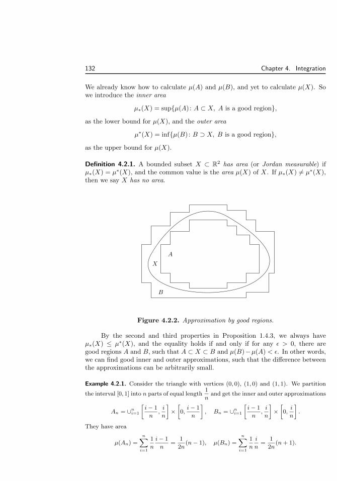
132 Chapter 4. Integration
We already know how to calculate µ(A) and µ(B), and yet to calculate µ(X). Sowe introduce the inner area
µ∗(X) = supµ(A) : A ⊂ X, A is a good region,
as the lower bound for µ(X), and the outer area
µ∗(X) = infµ(B) : B ⊃ X, B is a good region,
as the upper bound for µ(X).
Definition 4.2.1. A bounded subset X ⊂ R2 has area (or Jordan measurable) ifµ∗(X) = µ∗(X), and the common value is the area µ(X) of X. If µ∗(X) 6= µ∗(X),then we say X has no area.
B
X
A
Figure 4.2.2. Approximation by good regions.
By the second and third properties in Proposition 1.4.3, we always haveµ∗(X) ≤ µ∗(X), and the equality holds if and only if for any ε > 0, there aregood regions A and B, such that A ⊂ X ⊂ B and µ(B)−µ(A) < ε. In other words,we can find good inner and outer approximations, such that the difference betweenthe approximations can be arbitrarily small.
Example 4.2.1. Consider the triangle with vertices (0, 0), (1, 0) and (1, 1). We partition
the interval [0, 1] into n parts of equal length1
nand get the inner and outer approximations
An = ∪ni=1
[i− 1
n,i
n
]×[0,i− 1
n
], Bn = ∪ni=1
[i− 1
n,i
n
]×[0,i
n
].
They have area
µ(An) =
n∑i=1
1
n
i− 1
n=
1
2n(n− 1), µ(Bn) =
n∑i=1
1
n
i
n=
1
2n(n+ 1).

4.2. Darboux Integration 133
By taking sufficiently big n, the difference µ(Bn) − µ(An) =1
ncan be arbitrarily small.
Therefore the triangle has area, and the area is limn→∞ µ(An) = limn→∞ µ(Bn) =1
2.
1
inner approx.
1
outer approx.
Figure 4.2.3. Approximating triangle.
Example 4.2.2. For an example of subsets without area, i.e., satisfying µ∗(X) 6= µ∗(X),let us consider the subset X = (Q ∩ [0, 1])2 of all rational pairs in the unit square.
Since the only rectangles contained in X are single points, we have µ(A) = 0 for anygood region A ⊂ X. Therefore µ∗(X) = 0.
On the other hand, if B is a good region containing X, then B must almost containthe whole square [0, 1]2, with the only exception of finitely many horizontal or vertical linesegments. Therefore we have µ(B) ≥ µ([0, 1]2) = 1. This implies µ∗(X) ≥ 1 (show thatµ∗(X) = 1!).
Exercise 4.11. Explain that µ∗(X) = 0 implies X has zero area.
Exercise 4.12. Explain that finitely many points and straight line segments have zero area.
Exercise 4.13. Prove that X ⊂ Y implies µ∗(X) ≤ µ∗(Y ) and µ∗(X) ≤ µ∗(Y ). In particu-lar, we have µ(X) ≤ µ(Y ) in case both X and Y have areas.
Darboux Sum
A function f is Darboux integrable if region between the graph of the function andthe x-axis
G[a,b](f) = (x, y) : a ≤ x ≤ b, y is between 0 and f(x)
has area. LetH+ = (x, y) : y ≥ 0, H− = (x, y) : y ≤ 0
be the upper and lower half planes. Then we expect the intersections G[a,b](f)∩H+
and G[a,b](f) ∩H− also have areas, and the define the Darboux integral to be∫ b
a
f(x)dx = µ(G[a,b](f) ∩H+
)− µ
(G[a,b](f) ∩H−
).

134 Chapter 4. Integration
We use the same notation for the Darboux and Riemann integrals, because we willshow that the two integrals are equivalent.
For f ≥ 0, Figure 4.2.4 shows that, for any inner approximation, we can alwayschoose “full vertical strips” to get better (meaning larger) inner approximations forG[a,b](f). The same argument applies to outer approximations (here better meanssmaller). Therefore we only need to consider the approximations by full verticalstrips.
a b a bxi−1 xi
mi
Figure 4.2.4. Better inner approximations by vertical strips.
An approximation by full vertical strips is determined by a partition P ofthe interval [a, b]. On the i-th interval [xi−1, xi], the inner strip has height mi =inf [xi−1,xi] f , and the outer strip has height Mi = sup[xi−1,xi] f . Therefore the innerand outer approximations are
AP = ∪ni=1[xi−1, xi]× [0,mi) ⊂ X ⊂ BP = ∪ni=1[xi−1, xi]× [0,Mi].
The areas of the approximations the lower and upper Darboux sums
L(P, f) = µ(AP ) =
n∑i=1
mi(xi − xi−1),
U(P, f) = µ(BP ) =
n∑i=1
Mi(xi − xi−1).
Then we have the inner and outer areas of G[a,b](f)∫ b
a
f(x)dx = supall P
L(P, f),
∫ b
a
f(x)dx = infall P
U(P, f).
We call these the lower and upper Darboux integrals. The function is Darbouxintegrable if and only if the two Darboux integral are equal.
The concept of Darboux sum and Darboux integral can also be defined forany bounded (not necessarily non-negative) function.
Theorem 4.2.2. A bounded function f on a bounded interval [a, b] is Darboux in-tegrable if and only if for any ε > 0, there is a partition P , such that
U(P, f)− L(P, f) = ω(P, f) < ε.

4.2. Darboux Integration 135
The equality in the theorem uses
Mi −mi = sup[xi−1,xi]
f − inf[xi−1,xi]
f = ω[xi−1,xi](f).
Proof. By mi ≤ Mi, we always have L(P, f) ≤ U(P, f). Moreover, it is easy tosee that, if Q is a refinement of P , then L(P, f) ≤ L(Q, f) ≤ U(Q, f) ≤ U(P, f).Therefore for any partitions P and Q, we have
L(P, f) ≤ L(P ∪Q, f) ≤ U(P ∪Q, f) ≤ U(Q, f).
By the second property in Proposition 1.4.3, this implies
∫ b
a
f(x)dx ≤∫ b
a
f(x)dx.
Then by the third property in Proposition 1.4.3, f is Darboux integrable if and onlyif for any ε > 0, there are partitions P and Q, such that U(Q, f) − L(P, f) < ε.This is slightly weaker than the criterion in the theorem (which requires P = Q).On the other hand, if U(Q, f)− L(P, f) < ε, then
U(P ∪Q, f)− L(P ∪Q, f) ≤ U(Q, f)− L(P, f) < ε,
so that the stronger criterion is satisfied by P ∪Q.
We note that U(P, f)−L(P, f) is the area of the good region ∪ni=1[xi−1, xi]×[mi,Mi]. The good region can be regarded as an outer approximation of the graphof f . Therefore Theorem 4.2.2 basically means that the Darboux integrability isequivalent to that the graph of the function has zero area. A vast generalisation ofthis observation is the third property in Proposition 11.5.2.
Exercise 4.14. Prove that if Q is a refinement of P , then L(P, f) ≤ L(Q, f) ≤ U(Q, f) ≤U(P, f). Then use this to derive Exercise 4.6.
Exercise 4.15. Calculate the lower and upper Darboux integrals of the Dirichlet function.
Exercise 4.16. Prove that
∫ b
a
cf(x)dx = c
∫ b
a
f(x)dx and
∫ b
a
cf(x)dx = c
∫ b
a
f(x)dx for
c = 0.
Exercise 4.17. Prove that
∫ b
a
− f(x)dx = −∫ b
a
f(x)dx and
∫ b
a
− f(x)dx = −∫ b
a
f(x)dx for
c > 0.
Exercise 4.18. Prove that f ≥ g implies
∫ b
a
f(x)dx ≥∫ b
a
g(x)dx and
∫ b
a
f(x)dx ≥∫ b
a
g(x)dx.

136 Chapter 4. Integration
Exercise 4.19. Prove that
∫ b
a
(f(x) + g(x))dx ≥∫ b
a
f(x)dx +
∫ b
a
g(x)dx and
∫ b
a
(f(x) +
g(x))dx ≥∫ b
a
f(x)dx+
∫ b
a
g(x)dx. Moreover, show that the strict inequalities can happen.
Riemann v.s. Darboux
By Theorem 4.1.3, the Riemann integrability requires the Riemann sum of oscilla-tions to be small for all partitions P satisfying ‖P‖ < δ. In contrast, by Theorem4.2.2, the Darboux integrability only requires this for one partition. Therefore theRiemann integrability implies the Darboux integrability.
Theorem 4.2.3. A bounded function on a bounded interval is Riemann integrableif and only if it is Darboux integrable.
Proof. We need to prove that the Darboux integrability implies the Riemann inte-grability. Specifically, for any ε > 0, let a partition P satisfy ω(P, f) < ε. For anypartition Q, the common refinement P ∩Q is obtained by adding points of P to Q.If P has p partition points, then P ∩Q differs from Q on at most p intervals of Q,and the total length of such intervals in Q and in P ∪Q together is no more than2p‖Q‖. On the other hand, if f is bounded by B on the whole interval, then theoscillation of f on any smaller interval is ≤ 2B. Therefore
|ω(Q, f)− ω(P ∩Q, f)| ≤ 2B2p‖Q‖.
On the other hand, the refinement P ∩Q of P implies (see Exercise 4.6)
ω(P ∩Q, f) ≤ ω(P, f) < ε.
Therefore we conclude
ω(Q, f) ≤ ω(P ∩Q, f) + 4Bp‖Q‖ < ε+ 4Bp‖Q‖.
This implies (note that B and p are fixed)
‖Q‖ < δ =ε
4Bp=⇒ ω(Q, f) < 2ε,
which proves the Riemann criterion.
Exercise 4.20. Prove that∫ b
a
f(x)dx = lim‖P‖→0
U(P, f),
∫ b
a
f(x)dx = lim‖P‖→0
L(P, f).
The theory of area can be easily extended to the theory of volume for subsetsin Rn. The details are given in Section 11.4. A byproduct is the multivariableRiemann integral on subsets of Euclidean spaces. In contrast, the definition ofmultivariable Riemann integral in terms of Riemann sum is more cumbersome.
4.3. Property of Riemann Integration 137
The underlying idea of Darboux’s approach is area. This will lead to themodern measure theory, to be developed in Chapters 9, 10, 11, 12. In this sense,Darboux’s approach is superior to Riemann.
On the other hand, Darboux’s approach relies on the supremum and infimum,and therefore cannot be applied to the cases where there is no order (like vectorvalued functions) or the order is questionable (like Riemann-Stieltjes integral).
Finally, we remark that Darboux integral is the limit of the Riemann sumwith respect to the refinement of partitions. See Exercises 4.127 and 4.134.
4.3 Property of Riemann IntegrationDefined as a certain type of limit, the integration has properties analogous to thelimit of sequences and functions.
Proposition 4.3.1. Suppose f(x) and g(x) are integrable on [a, b]. Then f(x)+g(x)and cf(x) are also integrable on [a, b], and∫ b
a
(f(x) + g(x))dx =
∫ b
a
f(x)dx+
∫ b
a
g(x)dx,∫ b
a
cf(x)dx = c
∫ b
a
f(x)dx.
Proof. Let I =
∫ b
a
f(x)dx and J =
∫ b
a
g(x)dx. For any ε > 0, there is δ > 0, such
that‖P‖ < δ =⇒ |S(P, f)− I| < ε, |S(P, g)− J | < ε.
On the other hand, for the same partition P and the same sample points x∗i forboth f(x) and g(x), we have
S(P, f + g) =∑
(f(x∗i ) + g(x∗i ))∆xi
=∑
f(x∗i )∆xi +∑
g(x∗i )∆xi = S(P, f) + S(P, g).
Therefore
‖P‖ < δ =⇒ |S(P, f + g)− I − J | ≤ |S(P, f)− I|+ |S(P, g)− J | < 2ε.
This shows that f + g is also integrable, and
∫ b
a
(f(x) + g(x))dx = I+J . The proof
of
∫ b
a
cf(x)dx = cI is similar.
Example 4.3.1. Suppose f(x) and g(x) are integrable. By Proposition 4.3.1, f(x) + g(x)is integrable. By Proposition 4.1.6, f(x)2, g(x)2 and (f(x) + g(x))2 are also integrable.Then by Proposition 4.3.1 again, the product
f(x)g(x) =1
2
[(f(x) + g(x))2 − f(x)2 − g(x)2]
138 Chapter 4. Integration
is also integrable. However, there is no formula expressing the integral of f(x)g(x) in termsof the integrals of f(x) and g(x).
Moreover, if |g(x)| > c > 0 for a constant c, then by the discussion in Example 4.1.8,
the function1
g(x)is integrable, so that the quotient
f(x)
g(x)= f(x)
1
g(x)is also integrable.
A vast generalization of the example is given by Proposition 11.5.9, which basicallysays that a uniformly continuous combination of Riemann integrable functions is Riemannintegrable. Specifically, the product function φ(y, z) = yz is uniformly continuous on anybounded region of the plane. By the proposition, if f(x) and g(x) are Riemann integrable,then the composition φ(f(x), g(x)) = f(x)g(x) is Riemann integrable.
Example 4.3.2. Suppose f(x) is integrable on [a, b]. Suppose g(x) = f(x) for all x exceptat c ∈ [a, b]. Then g(x) = f(x) +λdc(x), where dc(x) is the function in Example 4.1.3 andλ = g(c)− f(c). By Example 4.1.3, g(x) is also integrable and∫ b
a
g(x)dx =
∫ b
a
f(x)dx+ λ
∫ b
a
dc(x)dx =
∫ b
a
f(x)dx.
The example shows that changing an integrable function at finitely many places doesnot change the integrability and the integral. In particular, it makes sense to talk aboutthe integrability of a function f(x) on a bounded open interval (a, b) because any numbersmay be assigned as f(a) and f(b) without affecting the integrability of (the extended) f(x)on [a, b].
Exercise 4.21. Prove that if f(x) and g(x) are integrable, then maxf(x), g(x) is alsointegrable.
Exercise 4.22. Suppose f(x) is integrable on [a, b]. Suppose cn ∈ [a, b] converges. Provethat if g(x) is obtained by modifying the values of f(x) at cn, and g(x) is still bounded,
then g(x) is Riemann integrable and
∫ b
a
g(x)dx =
∫ b
a
f(x)dx.
Proposition 4.3.2. Suppose f(x) and g(x) are integrable on [a, b]. If f(x) ≤ g(x),then ∫ b
a
f(x)dx ≤∫ b
a
g(x)dx.
Proof. Let I =
∫ b
a
f(x)dx and J =
∫ b
a
g(x)dx. For any ε > 0, there is δ > 0, such
that
‖P‖ < δ =⇒ |S(P, f)− I| < ε, |S(P, g)− J | < ε.
By choosing the same x∗i for both functions, we have
I − ε < S(P, f) =∑
f(x∗i )∆xi ≤∑
g(x∗i )∆xi = S(P, g) < J + ε.
Therefore we have the inequality I−ε < J+ε for any ε > 0. This implies I ≤ J .

4.3. Property of Riemann Integration 139
Example 4.3.3. If f(x) is integrable, then |f(x)| is integrable, and −|f(x)| ≤ f(x) ≤ |f(x)|.
By Proposition 4.3.2, we have −∫ b
a
|f(x)|dx ≤∫ b
a
f(x)dx ≤∫ b
a
|f(x)|dx. This is the same
as ∣∣∣∣∫ b
a
f(x)dx
∣∣∣∣ ≤ ∫ b
a
|f(x)|dx.
By inf [a,b] f ≤ f(x) ≤ sup[a,b] f , we also get
(b− a) inf[a,b]
f =
∫ b
a
(inf[a,b]
f
)dx ≤
∫ b
a
f(x)dx ≤∫ b
a
(sup[a,b]
f
)dx = (b− a) sup
[a,b]
f.
If f(x) is continuous, then this implies that the average1
b− a
∫ b
a
f(x)dx lies between the
maximum and the minimum of f(x), and by the Intermediate Value Theorem, we have∫ b
a
f(x)dx = f(c)(b− a) for some c ∈ [a, b].
Exercise 4.23. Suppose f(x) ≥ 0 is a concave function on [a, b]. Then for any y ∈ [a, b], f(x)is bigger than the function obtained by connecting straight lines from (a, 0) to (y, f(y))
and then to (b, 0). Use this to prove that f(y) ≤ 2
b− a
∫ b
a
f(x)dx. Moreover, determine
when the equality holds.
Exercise 4.24. Suppose f(x) is continuous on [a, b] and differentiable on (a, b). Suppose
m ≤ f ′ ≤ M on (a, b) and denote µ =f(b)− f(a)
b− a . By comparing f(x) with suitable
piecewise linear functions, prove that∣∣∣∣∫ b
a
f(x)dx− f(a) + f(b)
2(b− a)
∣∣∣∣ ≤ (M − µ)(µ−m)
2(M −m)(b− a)2.
Exercise 4.25 (First Integral Mean Value Theorem). Suppose f(x) is continuous on [a, b] andg(x) is non-negative and integrable on [a, b]. Prove that there is c ∈ [a, b], such that∫ b
a
g(x)f(x)dx = f(c)
∫ b
a
g(x)dx.
In fact, we can achieve this by c ∈ (a, b).
Exercise 4.26. Suppose f(x) is integrable on [a, b]. Prove that∣∣∣∣f(c)(b− a)−∫ b
a
f(x)dx
∣∣∣∣ ≤ ω[a,b](f)(b− a) for any c ∈ [a, b].
Exercise 4.27 (Integral Continuity). Suppose f(x) is a continuous function on an open inter-
val containing [a, b]. Prove that limt→0
∫ b
a
|f(x+ t)− f(x)|dx = 0. We will see in Exercise
4.90 that the continuity assumption is not needed.

140 Chapter 4. Integration
Proposition 4.3.3. Suppose f(x) is a function on [a, c], and b ∈ [a, c]. Then f(x)is integrable on [a, c] if and only if its restrictions on [a, b] and [b, c] are integrable.Moreover, ∫ c
a
f(x)dx =
∫ b
a
f(x)dx+
∫ c
b
f(x)dx.
The proposition reflects the intuition that, if a region is divided into non-overlapping parts, then the whole area is the sum of the areas of the parts.
Proof. The proof is based on the study of the relation of the Riemann sums of thefunction on [a, b], [b, c] and [a, c]. Let P be a partition of [a, c].
If P contains b as a partition point, then P is obtained by combining a partitionP ′ of [a, b] and a partition P ′′ of [b, c]. For any choice of x∗i for P and the samechoice for P ′ and P ′′, we have S(P, f) = S(P ′, f) + S(P ′′, f).
If P does not contain b as a partition point, then b ∈ (xk−1, xk) for somek, and the new partition P = P ∪ b is still obtained by combining a partitionP ′ of [a, b] and a partition P ′′ of [b, c] together. For any choice of x∗i for P , wekeep all x∗i with i 6= k and introduce x′
∗k ∈ [xk−1, b], x
′′∗k ∈ [b, xk] for P . Then
S(P , f) = S(P ′, f) + S(P ′′, f) as before, and
|S(P, f)− S(P ′, f)− S(P ′′, f)| = |S(P, f)− S(P , f)|= |f(x∗k)(xk − xk−1)− f(x′
∗k)(b− xk−1)− f(x′′
∗k)(xk − b)|
≤ 2
(sup
[xk−1,xk]
|f |
)‖P‖.
Suppose f is integrable on [a, b] and [b, c]. Then by Proposition 4.1.2, f(x)is bounded on the two intervals. Thus |f(x)| < B for some constant B and all
x ∈ [a, c]. Denote I =
∫ b
a
f(x)dx and J =
∫ c
b
f(x)dx. For any ε > 0, there is
δ > 0, such that for partitions P ′ of [a, b] and P ′′ of [b, c] satisfying ‖P ′‖ < δ and‖P ′′‖ < δ, we have |S(P ′, f)−I| < ε and |S(P ′′, f)−J | < ε. Then for any partitionP of [a, c] satisfying ‖P‖ < δ, we always have
|S(P, f)− I − J |≤ |S(P, f)− S(P ′, f)− S(P ′′, f)|+ |S(P ′, f)− I|+ |S(P ′′, f)− I|< 2Bδ + 2ε.
This implies that f(x) is integrable on [a, c], with
∫ c
a
f(x)dx = I + J .
It remains to show that the integrability on [a, c] implies the integrability on[a, b] and [b, c]. By the Cauchy criterion, for any ε > 0, there is δ > 0, such thatfor any partitions P and Q of [a, c] satisfying ‖P‖ < δ and ‖Q‖ < δ, we have|S(P, f) − S(Q, f)| < ε. Now suppose P ′ and Q′ are partitions of [a, b] satisfying‖P ′‖ < δ and ‖Q′‖ < δ. Let R be any partition of [b, c] satisfying ‖R‖ < δ. Byadding R to P ′ and Q′, we get partitions P and Q of [a, b] satisfying ‖P‖ < δ and

4.3. Property of Riemann Integration 141
‖Q‖ < δ. Moreover, the choices of x∗i (which may be different for P ′ and Q′) maybe extended by adding the same x∗i for R. Then we get
|S(P ′, f)− S(Q′, f)| = |(S(P ′, f) + S(R, f))− (S(Q′, f) + S(R, f))|= |S(P, f)− S(Q, f)| < ε.
This proves the integrability of f on [a, b]. The proof of the integrability on [b, c] issimilar.
Example 4.3.4. A function f(x) on [a, b] is a step function if there is a partition P andconstants ci, such that f(x) = ci on (xi−1, xi) (it does not matter what f(xi) are). Then∫ b
a
f(x)dx =∑∫ xi
xi−1
f(x)dx =∑∫ xi
xi−1
cidx =∑
ci(xi − xi−1).
Example 4.3.5. Suppose f(x) ≥ 0 is continuous on [a, b]. We claim that
limp→+∞
(∫ b
a
f(x)pdx
) 1p
= max[a,b]
f(x).
Let M = max[a,b] f(x). We have M = f(x0) for some x0 ∈ [a, b]. Since f(x) iscontinuous at x0, for any ε > 0, we have f(x) > M − ε on an interval [c, d] containing x0.Then
Mp(b− a) ≥∫ b
a
f(x)pdx =
(∫ c
a
+
∫ d
c
+
∫ b
d
)f(x)pdx
≥∫ d
c
f(x)pdx ≥ (M − ε)p(d− c).
Therefore
M(b− a)1p ≥
(∫ b
a
f(x)pdx
) 1p
≥ (M − ε)(d− c)1p .
As p→ +∞, the left side converges to M and the right side converges to M− ε. Thereforethere is N , such that
p > N =⇒ M + ε > M(b− a)1p , (M − ε)(d− c)
1p > M − 2ε
=⇒ M + ε >
(∫ b
a
f(x)pdx
) 1p
> M − 2ε.
This proves that limp→+∞
(∫ b
a
f(x)pdx
) 1p
= M .
Example 4.3.6 (Testing Function). Suppose f(x) is continuous on [a, b]. If
∫ b
a
f(x)g(x)dx =
0 for any continuous function g(x), we prove that f(x) = 0 everywhere.Suppose f(c) > 0 for some c ∈ [a, b]. By the continuity of f(x) at c, there is δ > 0,
such that f(x) >1
2f(c) on (c− 2δ, c+ 2δ). Then we construct a continuous function g(x)
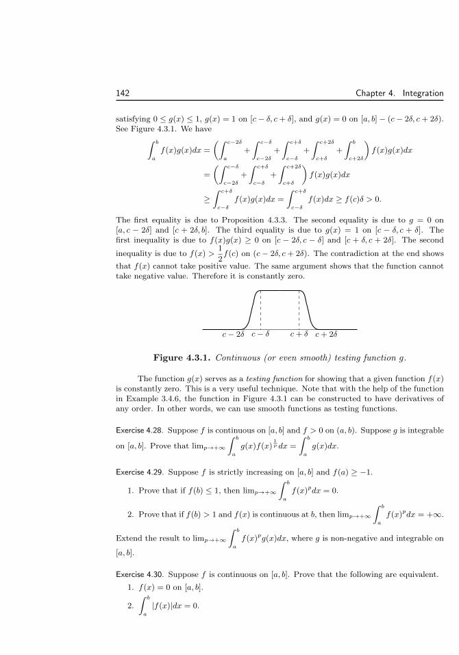
142 Chapter 4. Integration
satisfying 0 ≤ g(x) ≤ 1, g(x) = 1 on [c− δ, c+ δ], and g(x) = 0 on [a, b]− (c− 2δ, c+ 2δ).See Figure 4.3.1. We have∫ b
a
f(x)g(x)dx =
(∫ c−2δ
a
+
∫ c−δ
c−2δ
+
∫ c+δ
c−δ+
∫ c+2δ
c+δ
+
∫ b
c+2δ
)f(x)g(x)dx
=
(∫ c−δ
c−2δ
+
∫ c+δ
c−δ+
∫ c+2δ
c+δ
)f(x)g(x)dx
≥∫ c+δ
c−δf(x)g(x)dx =
∫ c+δ
c−δf(x)dx ≥ f(c)δ > 0.
The first equality is due to Proposition 4.3.3. The second equality is due to g = 0 on[a, c − 2δ] and [c + 2δ, b]. The third equality is due to g(x) = 1 on [c − δ, c + δ]. Thefirst inequality is due to f(x)g(x) ≥ 0 on [c − 2δ, c − δ] and [c + δ, c + 2δ]. The second
inequality is due to f(x) >1
2f(c) on (c− 2δ, c+ 2δ). The contradiction at the end shows
that f(x) cannot take positive value. The same argument shows that the function cannottake negative value. Therefore it is constantly zero.
c− δ c+ δc− 2δ c+ 2δ
Figure 4.3.1. Continuous (or even smooth) testing function g.
The function g(x) serves as a testing function for showing that a given function f(x)is constantly zero. This is a very useful technique. Note that with the help of the functionin Example 3.4.6, the function in Figure 4.3.1 can be constructed to have derivatives ofany order. In other words, we can use smooth functions as testing functions.
Exercise 4.28. Suppose f is continuous on [a, b] and f > 0 on (a, b). Suppose g is integrable
on [a, b]. Prove that limp→+∞
∫ b
a
g(x)f(x)1p dx =
∫ b
a
g(x)dx.
Exercise 4.29. Suppose f is strictly increasing on [a, b] and f(a) ≥ −1.
1. Prove that if f(b) ≤ 1, then limp→+∞
∫ b
a
f(x)pdx = 0.
2. Prove that if f(b) > 1 and f(x) is continuous at b, then limp→+∞
∫ b
a
f(x)pdx = +∞.
Extend the result to limp→+∞
∫ b
a
f(x)pg(x)dx, where g is non-negative and integrable on
[a, b].
Exercise 4.30. Suppose f is continuous on [a, b]. Prove that the following are equivalent.
1. f(x) = 0 on [a, b].
2.
∫ b
a
|f(x)|dx = 0.
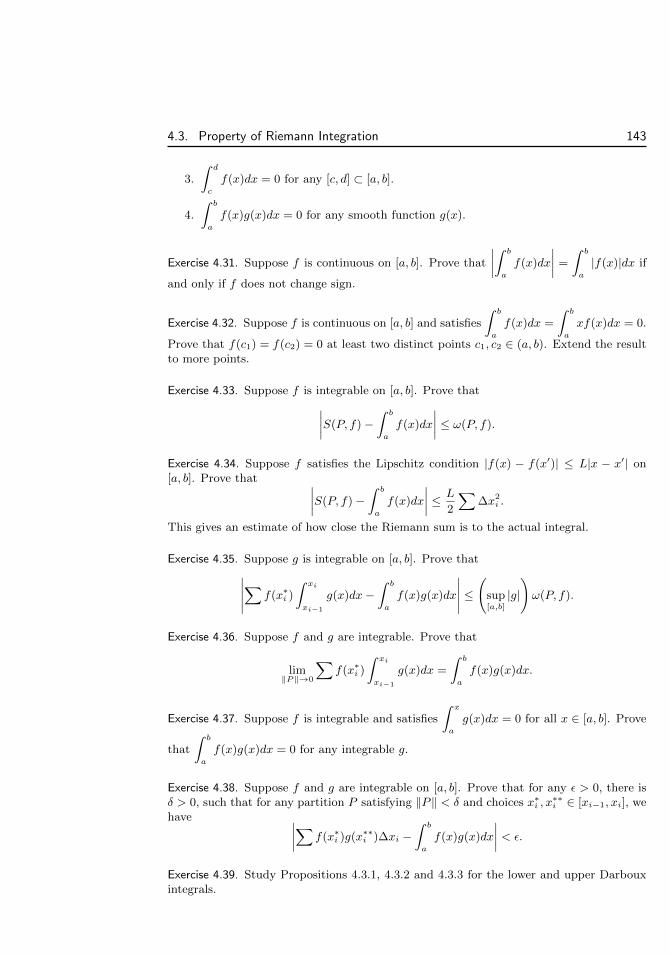
4.3. Property of Riemann Integration 143
3.
∫ d
c
f(x)dx = 0 for any [c, d] ⊂ [a, b].
4.
∫ b
a
f(x)g(x)dx = 0 for any smooth function g(x).
Exercise 4.31. Suppose f is continuous on [a, b]. Prove that
∣∣∣∣∫ b
a
f(x)dx
∣∣∣∣ =
∫ b
a
|f(x)|dx if
and only if f does not change sign.
Exercise 4.32. Suppose f is continuous on [a, b] and satisfies
∫ b
a
f(x)dx =
∫ b
a
xf(x)dx = 0.
Prove that f(c1) = f(c2) = 0 at least two distinct points c1, c2 ∈ (a, b). Extend the resultto more points.
Exercise 4.33. Suppose f is integrable on [a, b]. Prove that∣∣∣∣S(P, f)−∫ b
a
f(x)dx
∣∣∣∣ ≤ ω(P, f).
Exercise 4.34. Suppose f satisfies the Lipschitz condition |f(x) − f(x′)| ≤ L|x − x′| on[a, b]. Prove that ∣∣∣∣S(P, f)−
∫ b
a
f(x)dx
∣∣∣∣ ≤ L
2
∑∆x2
i .
This gives an estimate of how close the Riemann sum is to the actual integral.
Exercise 4.35. Suppose g is integrable on [a, b]. Prove that∣∣∣∣∣∑ f(x∗i )
∫ xi
xi−1
g(x)dx−∫ b
a
f(x)g(x)dx
∣∣∣∣∣ ≤(
sup[a,b]
|g|
)ω(P, f).
Exercise 4.36. Suppose f and g are integrable. Prove that
lim‖P‖→0
∑f(x∗i )
∫ xi
xi−1
g(x)dx =
∫ b
a
f(x)g(x)dx.
Exercise 4.37. Suppose f is integrable and satisfies
∫ x
a
g(x)dx = 0 for all x ∈ [a, b]. Prove
that
∫ b
a
f(x)g(x)dx = 0 for any integrable g.
Exercise 4.38. Suppose f and g are integrable on [a, b]. Prove that for any ε > 0, there isδ > 0, such that for any partition P satisfying ‖P‖ < δ and choices x∗i , x
∗∗i ∈ [xi−1, xi], we
have ∣∣∣∣∑ f(x∗i )g(x∗∗i )∆xi −∫ b
a
f(x)g(x)dx
∣∣∣∣ < ε.
Exercise 4.39. Study Propositions 4.3.1, 4.3.2 and 4.3.3 for the lower and upper Darbouxintegrals.

144 Chapter 4. Integration
The definition of the Riemann integral
∫ b
a
f(x)dx implicitly assumes a < b.
If a > b, then we also define∫ b
a
f(x)dx = −∫ a
b
f(x)dx.
Moreover, we define
∫ a
a
f(x)dx = 0 (which can be considered as a special case of
the original definition of the Riemann integral). Then the equality∫ c
a
f(x)dx =
∫ b
a
f(x)dx+
∫ c
b
f(x)dx
still holds for any order between a, b, c. Proposition 4.3.1 still holds for a ≥ b, andthe direction of the inequality in Proposition 4.3.2 needs to be reversed for a ≥ b.
4.4 Fundamental Theorem of CalculusThe integration was originally considered as the inverse of the differentiation. Suchconnection between integration and differentiation is the Fundamental Theorem ofCalculus.
Newton-Leibniz Formula
Theorem 4.4.1. Suppose F (x) is continuous on [a, b], differentiable on (a, b), and
F ′(x) is integrable. Then F (x) = F (a) +
∫ x
a
F ′(t)dt.
Proof. Let P be a partition of [a, b]. By the Mean Value Theorem, we can expressF (b)− F (a) as a Riemann sum of F ′(x) with suitable choice of x∗i
F (b)− F (a) =∑
(F (xi)− F (xi−1)) =∑
F ′(x∗i )(xi − xi−1).
By the integrability of F ′(x), the right side converges to
∫ b
a
F ′(x)dx as ‖P‖ → 0.
Therefore F (b)− F (a) =
∫ b
a
F ′(x)dx.
The theorem tells us that, if f(x) is integrable and F (x) is an antiderivative off (meaning F is differentiable and F ′(x) = f(x)), then we have the Newton-Leibnizformula for calculating the integral of f∫ b
a
f(x)dx = F (b)− F (a).
This raises two questions.
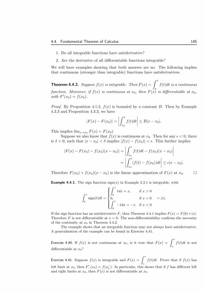
4.4. Fundamental Theorem of Calculus 145
1. Do all integrable functions have antiderivative?
2. Are the derivative of all differentiable functions integrable?
We will have examples showing that both answers are no. The following impliesthat continuous (stronger than integrable) functions have antiderivatives.
Theorem 4.4.2. Suppose f(x) is integrable. Then F (x) =
∫ x
a
f(t)dt is a continuous
function. Moreover, if f(x) is continuous at x0, then F (x) is differentiable at x0,with F ′(x0) = f(x0).
Proof. By Proposition 4.1.2, f(x) is bounded by a constant B. Then by Example4.3.3 and Proposition 4.3.3, we have
|F (x)− F (x0)| =∣∣∣∣∫ x
x0
f(t)dt
∣∣∣∣ ≤ B|x− x0|.
This implies limx→x0F (x) = F (x0).
Suppose we also know that f(x) is continuous at x0. Then for any ε < 0, thereis δ > 0, such that |x− x0| < δ implies |f(x)− f(x0)| < ε. This further implies
|F (x)− F (x0)− f(x0)(x− x0)| =∣∣∣∣∫ x
x0
f(t)dt− f(x0)(x− x0)
∣∣∣∣=
∣∣∣∣∫ x
x0
(f(t)− f(x0))dt
∣∣∣∣ ≤ ε|x− x0|.
Therefore F (x0) + f(x0)(x− x0) is the linear approximation of F (x) at x0.
Example 4.4.1. The sign function sign(x) in Example 2.3.1 is integrable, with
∫ x
0
sign(t)dt =
∫ x
0
1dx = x, if x > 0
0, if x = 0∫ x
0
−1dx = −x if x < 0
= |x|.
If the sign function has an antiderivative F , then Theorem 4.4.1 implies F (x) = F (0)+ |x|.Therefore F is not differentiable at x = 0. The non-differentiability confirms the necessityof the continuity at x0 in Theorem 4.4.2.
The example shows that an integrable function may not always have antiderivative.A generalisation of the example can be found in Exercise 4.41.
Exercise 4.40. If f(x) is not continuous at x0, is it true that F (x) =
∫ x
a
f(t)dt is not
differentiable at x0?
Exercise 4.41. Suppose f(x) is integrable and F (x) =
∫ x
a
f(t)dt. Prove that if f(x) has
left limit at x0, then F ′−(x0) = f(x−0 ). In particular, this shows that if f has different leftand right limits at x0, then F (x) is not differentiable at x0.

146 Chapter 4. Integration
Exercise 4.42. Suppose f(x) is integrable on [a, b]. Prove that1
2
∫ b
a
f(x)dx =
∫ c
a
f(x)dx
for some c ∈ (a, b). Can1
2be replaced by some other number?
Example 4.4.2. The function
F (x) =
x2 sin1
x, if x 6= 0,
0, if x = 0,
is differentiable, and its derivative function
f(x) =
2x sin1
x− cos
1
x, if x 6= 0,
0, if x = 0,
is not continuous but still integrable by Proposition 4.1.4 and Exercise 4.7. Therefore we
still have the Newton-Leibniz formula
∫ 1
0
f(x)dx = F (1)− F (0) = sin 1.
Example 4.4.3. The function
F (x) =
x2 sin1
x2, if x 6= 0,
0, if x = 0,
is differentiable, and its derivative function
f(x) =
2x sin1
x2− 2
xcos
1
x2, if x 6= 0,
0, if x = 0,
is not integrable on [0, 1] because it is not bounded.The example appears to tell us that derivative functions are not necessarily inte-
grable. However, such interpretation is misleading because the problem is not the failureof the integrability criterion, but that the integration is not defined for unbounded function.One natural way to extend the integration to unbounded functions is through improperintegral, which is defined as the limit of the integration of the bounded part∫ 1
0
f(x)dx = lima→0+
∫ 1
a
f(x)dx = lima→0+
(F (1)− F (a)) = F (1)− F (0) = sin 1.
The example suggests that, by suitably extending the integration, derivative func-tions are likely to be always integrable. Moreover, the current example, Example 4.4.2,and Exercise 4.43 suggests that the Newton-Leibniz formula are likely always true in theextended integration theory.
Exercise 4.43. Prove that Theorem 4.4.1 still holds for piecewise differentiable. In otherwords, if F is continuous, differentiable at all but finitely many points, and F ′ is integrable,then the Newton-Leibniz formula remains true.
Exercise 4.44. Suppose F is continuous on [a, b] and differentiable on (a, b). Suppose F (x) =
F (a) +
∫ x
a
f(t)dt for an integrable f and all x ∈ (a, b).

4.4. Fundamental Theorem of Calculus 147
1. Prove that on any interval [c, d] ⊂ [a, b], we have inf [c,d] f ≤ F ′(x) ≤ sup[c,d] f forany x ∈ [c, d]. In other words, the derivative F ′ is bounded by the bounds of f .
2. Prove that F ′ is integrable on [a, b].
Combined with Theorem 4.4.1, the second statement gives the necessary and sufficientcondition for the integrability of F ′.
Exercise 4.45. Explain that the function f in Exercise 4.44 is not necessarily equal to F ′.Then use Exercise 4.37 to compare f and F ′.
If the answers to both questions after Theorem 4.4.1 are affirmative, thenwe would have the perfect Fundamental Theorem. The examples and exercisesabove show that, although the Fundamental Theorem for Riemann integral is notperfect, the problem happens only at few places. They also suggest that, if theintegration can be extended to tolerate “small defects”, then it is possible to getperfect Fundamental Theorem. This is realised by Theorem 12.3.5, in the settingof Lebesgue integral.
Application of Fundamental Theorem
Example 4.4.4. We try to find continuous f(x) on [0,+∞), such that p
∫ x
0
tf(t)dt =
x
∫ x
0
f(t)dt. The continuity means that we can take derivative on both sides and get
pxf(x) = xf(x) +
∫ x
0
f(t)dt, or (p− 1)xf(x) =
∫ x
0
f(t)dt.
If p = 1, then
∫ x
0
f(t)dt = 0 for all x ≥ 0. This means f(x) is constantly zero.
If p 6= 1, then the differentiability of
∫ x
0
f(t)dt implies the differentiability of f(x) =
1
(p− 1)x
∫ x
0
f(t)dt for x > 0. By taking derivative of both sides of (p − 1)xf(x) =∫ x
0
f(t)dt, we get (p− 1)(f(x) + xf ′(x)) = f(x), or qf(x) + xf ′(x) = 0, where q =p− 2
p− 1.
This means (xqf(x))′ = qxq−1f(x) + xqf(x) = xq−1(qf(x) + xf ′(x)) = 0. Therefore we
find that xqf(x) = c is a constant, or f(x) = cx2−pp−1 . We note that, in order for the integral
on [0, x] to make sense, f(x) has to be bounded on bounded intervals. This means that
we need to have2− pp− 1
≥ 0, or 1 < p ≤ 2. In this case, substituting f(x) = cx2−pp−1 into the
original equation shows that it is indeed a solution.
We conclude that, if 1 < p ≤ 2, then the solutions are f(x) = cx2−pp−1 . Otherwise,
the only solution is f(x) = 0.
Exercise 4.46. Find continuous functions satisfying the equalities.
1.
∫ x
0
f(t)dt =
∫ 1
x
f(t)dt on [0, 1].
2. p
∫ x
1
tf(t)dt = x
∫ x
1
f(t)dt on (0,+∞).

148 Chapter 4. Integration
3. (f(x))2 = 2
∫ x
0
f(t)dt on (−∞,+∞).
Exercise 4.47. Find continuous functions f(x) on (0,+∞), such that for all b > 0, the
integral
∫ ab
a
f(x)dx is independent of a > 0.
Since integration is almost the converse of differentiation, the properties ofdifferentiation should have integration counterparts. The counterpart of (f + g)′ =f ′ + g′ and (cf)′ = cf ′ is Proposition 4.3.1. The counterpart of the Leibniz rule isthe following.
Theorem 4.4.3 (Integration by Parts). Suppose f(x), g(x) are differentiable, andf ′(x), g′(x) are integrable. Then∫ b
a
f(x)g′(x)dx+
∫ b
a
f ′(x)g(x)dx = f(b)g(b)− f(a)g(a).
Since the current Fundamental Theorem is not perfect, the integration byparts in the theorem is not the best we can get. Theorem 4.5.3 gives the bestversion.
Proof. Since differentiability implies continuity (Proposition 3.1.3), and continuityimplies integrability (Proposition 4.1.4), we know f, g are integrable. Then byExample 4.3.1, fg′, f ′g are integrable, and (fg)′ = fg′ + f ′g is integrable. ByTheorem 4.4.1, we get∫ b
a
f(x)g′(x)dx+
∫ b
a
f ′(x)g(x)dx =
∫ b
a
(f(x)g(x))′dx = f(b)g(b)− f(a)g(a).
The chain rule also has its integration counterpart.
Theorem 4.4.4 (Change of Variable). Suppose φ(x) is differentiable, with φ′(x) in-tegrable on [a, b]. Suppose f(y) is continuous on φ([a, b]). Then∫ φ(b)
φ(a)
f(y)dy =
∫ b
a
f(φ(x))φ′(x)dx.
Again the theorem is not the best change of variable formula we can get.Theorem 4.5.4 gives the best version. Moreover, Exercise 4.65 gives another versionof change of variable, with more strict condition on φ and less strict condition onf .
Proof. Applying Theorem 4.4.2 to the continuous f , we find that F (z) =
∫ z
φ(a)
f(y)dy
satisfies F ′(z) = f(z). Since φ is differentiable, by the chain rule, we have
F (φ(x))′ = F ′(φ(x))φ′(x) = f(φ(x))φ′(x).

4.4. Fundamental Theorem of Calculus 149
Since f and φ are continuous, the composition f(φ(x)) is continuous and thereforeintegrable. Moreover, φ′(x) is assumed to be integrable. Therefore the productf(φ(x))φ′(x) is integrable, and we may apply Theorem 4.4.1 to get
F (φ(b))− F (φ(a)) =
∫ b
a
f(φ(x))φ′(x)dx.
By the definition of F (z), this is the equality in the theorem.
Exercise 4.48 (Jean Bernoulli24). Suppose f(t) has continuous n-th order derivative on [0, x].Prove that∫ x
0
f(t)dt = xf(x)− x2
2!f ′(x) + · · ·+ (−1)n−1 x
n
n!f (n−1)(x) + (−1)n
1
n!
∫ x
0
tnf (n)(t)dt.
Exercise 4.49. Suppose u(x) and v(x) have continuous n-th order derivatives on [a, b]. Provethat∫ b
a
uv(n)dx =[uv(n−1) − u′v(n−2) + · · ·+ (−1)n−1u(n−1)v
]x=b
x=a+ (−1)n
∫ b
a
u(n)vdx.
Then apply the formula to
∫ x
x0
(x−t)nf (n+1)(t)dt to prove the integral form of the remainder
of the Taylor expansion
Rn(x) =1
n!
∫ x
x0
(x− t)nf (n+1)(t)dt.
Exercise 4.50. Suppose f ′(x) is integrable and limx→+∞ f′(x) = 0. Prove that
limb→+∞
1
b
∫ b
a
f(x) sinxdx = 0.
Moreover, extend the result to high order derivatives.
Exercise 4.51. Suppose f(x) is continuous on [−a, a]. Prove that the following are equiva-lent.
1. f(x) is an odd function.
2.
∫ b
−bf(x)dx = 0 for any 0 < b < a.
3.
∫ a
−af(x)g(x)dx = 0 for any even continuous function g(x).
4.
∫ a
−af(x)g(x)dx = 0 for any even integrable function g(x).
Exercise 4.52. Suppose f(x) is integrable on [0, 1] and is continuous at 0. Prove that
limh→0+
∫ 1
0
h
h2 + x2f(x)dx =
π
2f(0).
24Jean Bernoulli, born 1667 and died 1748 in Basel (Switzerland).

150 Chapter 4. Integration
Exercise 4.53. Suppose f(x) is integrable on an open interval containing [a, b] and is con-tinuous at a and b. Prove that
limh→0
∫ b
a
f(x+ h)− f(x)
hdx = f(b)− f(a).
The result should be compared with the equality∫ b
a
limh→0
f(x+ h)− f(x)
hdx =
∫ b
a
f ′(x)dx = f(b)− f(a),
which by Theorem 4.4.1 holds when f(x) is differentiable and f ′(x) is integrable.
4.5 Riemann-Stieltjes Integration
Riemann-Stieltjes Sum
Let f and α be functions on a bounded interval [a, b]. The Riemann-Stieltjes25 sumof f with respect to α is
S(P, f, α) =
n∑i=1
f(x∗i )(α(xi)− α(xi−1)) =
n∑i=1
f(x∗i )∆αi.
We say that f has Riemann-Stieltjes integral I and denote
∫ b
a
fdα = I, if for any
ε > 0, there is δ > 0, such that
‖P‖ < δ =⇒ |S(P, f, α)− I| < ε.
When α(x) = x, we get the Riemann integral.
Example 4.5.1. Suppose f(x) = c is a constant. Then S(P, f, α) = c(α(b)−α(a)). There-
fore
∫ b
a
cdα = c(α(b)− α(a)).
Example 4.5.2. Suppose α(x) = α0 is a constant. Then ∆αi = 0, and therefore
∫ b
a
fdα0 =
0 for any f . Since f can be arbitrary, we see that Proposition 4.1.2 cannot be extendedwithout additional conditions.
Example 4.5.3. Suppose the Dirichlet function D(x) is Riemann-Stieltjes integrable withrespect to α on [a, b]. We claim that α must be a constant.
Let c, d ∈ [a, b], c < d. Let P be any partition with c and d as partition points. If wechoose all x∗i to be irrational, then we get S(P,D, α) = 0. If we choose x∗i to be irrationalwhenever [xi−1, xi] 6⊂ [c, d] and choose x∗i to be rational whenever [xi−1, xi] ⊂ [c, d], thenwe get S(P,D, α) = α(d)−α(c). Since the two choices should converge to the same limit,we conclude that α(d)−α(c) = 0. Since c, d are arbitrary, we conclude that α is a constant.
25Thomas Jan Stieltjes, born 1856 in Zwolle (Netherland), died 1894 in Toulouse (France). Heis often called the father of the analytic theory of continued fractions and is best remembered forhis integral.

4.5. Riemann-Stieltjes Integration 151
The example shows that it is possible for a nonzero function f to satisfy
∫ b
a
fdα = 0
whenever the Riemann-Stieltjes integral makes sense.
Exercise 4.54. Prove that the only function that is Riemann-Stieltjes integrable with re-spect to the Dirichlet function is the constant function. In particular, this shows that∫ b
a
fdα = 0 for any function f that is Riemann-Stieltjes integrable with respect to α does
not necessarily imply that α is a constant.
Exercise 4.55. Suppose c ∈ (a, b), the three numbers α−, α0, α+ are not all equal, and
α(x) =
α−, if x < c,
α0, if x = c,
α+, if x > c.
Prove that f is Riemann-Stieltjes integrable with respect to α if and only if f is continuous
at c. Moreover, we have
∫ b
a
fdα = f(c)(α+ − α−).
Exercise 4.56. Find suitable α on [0, 2], such that
∫ 2
0
fdα = f(0) + f(1) + f(2) for any
continuous f on [0, 2].
Proposition 4.5.1. Suppose f is Riemann-Stieltjes integrable with respect to α on[a, b]. Then at any c ∈ [a, b], either f or α is continuous at c.
Proof. The Cauchy criterion for the convergence of Riemann-Stieltjes sum is that,for any ε > 0, there is δ > 0, such that
‖P‖ < δ, ‖P ′‖ < δ =⇒ |S(P, f, α)− S(P ′, f, α)| < ε.
For x ≤ u ≤ v ≤ y satisfying |x− y| < δ, we choose P to be a partition with [x, y]as a partition interval and with u ∈ [x, y] as a sample point. We also choose P ′ tobe the same partition, with the same sample points except u is replaced by v. Thenwe get
S(P, f, α)− S(P ′, f, α) = (f(u)− f(v))(α(y)− α(x)),
and the Cauchy criterion specialises to
x ≤ u ≤ v ≤ y, |x− y| < δ =⇒ |f(u)− f(v)| |α(x)− α(y)| < ε.
Now we study what happens at c ∈ [a, b]. If α is not continuous at c, theneither limx→c α(x) diverges, or the limit converges but is not equal to α(c). Wewant to show that f is continuous at c in either case.
Suppose limx→c α(x) diverges. By Exercise 2.14, there is B > 0, such that
for the δ > 0 above, we can find x, y satisfying c − δ
2< x < c < y < c +
δ
2and

152 Chapter 4. Integration
|α(x)− α(y)| ≥ B. Note that B depends only on α and c, and is independent of δand ε. Since |x− y| < δ, we get
u, v ∈ [x, y] =⇒ |f(u)− f(v)| < ε
|α(x)− α(y)|<
ε
B.
By x < c < y, we can find δ′, such that x < c− δ′ < c < c+ δ′ < y. Then by takingv = c, the implication above further implies
|u− c| < δ′ =⇒ |f(u)− f(c)| < ε
B.
This verifies the continuity of f at c.Suppose limx→c α(x) converges but is not equal to α(c). By limx→c+ α(x) 6=
α(c), there is B > 0, such that for the δ > 0 above, we can find y satisfyingc < y < c+ δ and |α(c)− α(y)| ≥ B. Since |y − c| < δ, we get
u, v ∈ [c, y] =⇒ |f(u)− f(v)| < ε
|α(c)− α(y)|<
ε
B.
Let δ′ = y − c. Then by taking v = c, the implication above further implies
0 ≤ u− c < δ′ =⇒ |f(u)− f(c)| < ε
B.
This verifies the right continuity of f at c. By the same reason, f is also leftcontinuous at c.
Property of Riemann-Stieltjes Integral
Many properties of the Riemann integral can be extended to Riemann-Stieltjesintegral. Sometimes one needs to be careful with the continuity condition fromProposition 4.5.1. When it comes to inequality, we may also need α to be monotone.
Exercise 4.57. Suppose f and g are Riemann-Stieltjes integrable with respect to α. Provethat f + g and cf are Riemann-Stieltjes integrable with respect to α and∫ b
a
(f + g)dα =
∫ b
a
fdα+
∫ b
a
gdα,
∫ b
a
cfdα = c
∫ b
a
fdα.
This extends Proposition 4.3.1.
Exercise 4.58. Suppose f is Riemann-Stieltjes integrable with respect to α and β. Supposec is a constant. Prove that f is Riemann-Stieltjes integrable with respect to α+β and cα,and ∫ b
a
fd(α+ β) =
∫ b
a
fdα+
∫ b
a
fdβ,
∫ b
a
fd(cα) = c
∫ b
a
fdα.
Exercise 4.59. Suppose f and α are functions on [a, c] and b ∈ (a, c).
1. Prove that if f is Riemann-Stieltjes integrable with respect to α on [a, c], then f isRiemann-Stieltjes integrable with respect to α on [a, b] and [b, c], and∫ c
a
fdα =
∫ b
a
fdα+
∫ c
b
fdα.

4.5. Riemann-Stieltjes Integration 153
2. Suppose f and α are bounded, and either f or α is continuous at c. Prove thatif f is Riemann-Stieltjes integrable with respect to α on [a, b] and [b, c], then f isRiemann-Stieltjes integrable with respect to α on [a, c].
3. Construct bounded functions f and α, such that f is Riemann-Stieltjes integrablewith respect to α on [a, b] and [b, c], but f is left continuous and not right continuousat c, while α is right continuous and not left continuous at c. By Exercise 4.55, f isnot Riemann-Stieltjes integrable with respect to α on [a, c].
This shows that Proposition 4.3.3 may be extended as long as either f or α is continuousat the breaking point c.
Exercise 4.60. Suppose f and g are Riemann-Stieltjes integrable with respect to an increas-ing α on [a, b]. Prove that
f ≤ g =⇒∫ b
a
fdα ≤∫ b
a
gdα.
Moreover, if α is strictly increasing and f and g are continuous, then the equality holdsif and only if f = g. This shows that Proposition 4.3.2 may be extended as long as weassume that α is increasing.
Exercise 4.61. Suppose f is Riemann-Stieltjes integrable with respect to an increasing αon [a, b]. Prove that ∣∣∣∣∫ b
a
fdα
∣∣∣∣ ≤ ∫ b
a
|f |dα,
(α(b)− α(a)) inf[a,b]
f ≤∫ b
a
fdα ≤ (α(b)− α(a)) sup[a,b]
f,∣∣∣∣f(c)(α(b)− α(a))−∫ b
a
fdα
∣∣∣∣ ≤ ω[a,b](f)(α(b)− α(a)) for c ∈ [a, b],∣∣∣∣S(P, f, α)−∫ b
a
fdα
∣∣∣∣ ≤∑ω[xi−1,xi](f)∆αi.
Moreover, extend the first Integral Mean Value Theorem in Exercise 4.25 to the Riemann-Stieltjes integral.
Exercise 4.62. Suppose f is Riemann-Stieltjes integrable with respect to α, and F (x) =∫ x
a
fdα. Prove that if α is monotone and f is continuous at x0, then for any ε > 0, there
is δ > 0, such that
|∆x| = |x− x0| < δ =⇒ |F (x)− F (x0)− f(x0)∆α| ≤ ε|∆α|.
This shows that the Fundamental Theorem of Calculus may be extended as long as α ismonotone.
The following is the relation between Riemann-Stieltjes integral and the or-dinary Riemann integral. An extension is given in Exercise 4.77. A much moregeneral extension is given by Example 12.4.1.

154 Chapter 4. Integration
Theorem 4.5.2. Suppose f is bounded, g is Riemann integrable, and α(x) = α(a)+∫ x
a
g(t)dt. Then f is Riemann-Stieltjes integrable with respect to α if and only if
fg is Riemann integrable. Moreover,∫ b
a
fdα =
∫ b
a
fgdx.
For the special case α is differentiable with Riemann integrable α′, by Theorem4.4.1, the formula becomes ∫ b
a
fdα =
∫ b
a
fα′dx.
This is consistent with the notation dα = α′dx for the differential.
Proof. Suppose |f | < B for a constant B. Since g is Riemann integrable, for anyε > 0, there is δ > 0, such that ‖P‖ < δ implies
∑ω[xi−1,xi](g)∆xi < ε. For the
same choice of P and x∗i , the Riemann-Stieltjes sum of f with respect to α is
S(P, f, α) =∑
f(x∗i )(α(xi)− α(xi−1)) =∑
f(x∗i )
∫ xi
xi−1
g(t)dt.
The Riemann sum of fg is
S(P, fg) =∑
f(x∗i )g(x∗i )∆xi.
When ‖P‖ < δ, we have (the second inequality uses Exercise 4.26)
|S(P, f, α)− S(P, fg)| ≤∑|f(x∗i )|
∣∣∣∣∣∫ xi
xi−1
g(t)dt− g(x∗i )∆xi
∣∣∣∣∣≤∑
Bω[xi−1,xi](g)∆xi ≤ Bε.
This implies that the Riemann-Stieltjes sum of f with respect to α converges ifand only if the Riemann sum of fg converges. Moreover, the two limits are thesame.
The following shows that, in a Riemann-Stieltjes integral
∫ b
a
fdα, the roles of
f and α may be exchanged.
Theorem 4.5.3 (Integration by Parts). A function f is Riemann-Stieltjes integrablewith respect to α if and only if α is Riemann-Stieltjes integrable with respect to f .Moreover, ∫ b
a
fdα+
∫ b
a
αdf = f(b)α(b)− f(a)α(a).
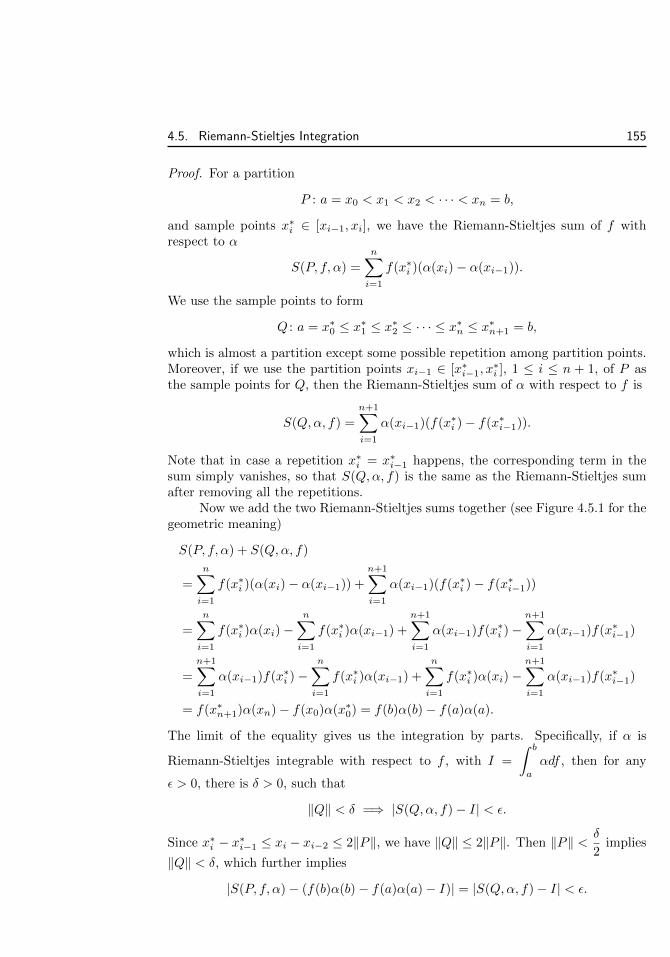
4.5. Riemann-Stieltjes Integration 155
Proof. For a partition
P : a = x0 < x1 < x2 < · · · < xn = b,
and sample points x∗i ∈ [xi−1, xi], we have the Riemann-Stieltjes sum of f withrespect to α
S(P, f, α) =
n∑i=1
f(x∗i )(α(xi)− α(xi−1)).
We use the sample points to form
Q : a = x∗0 ≤ x∗1 ≤ x∗2 ≤ · · · ≤ x∗n ≤ x∗n+1 = b,
which is almost a partition except some possible repetition among partition points.Moreover, if we use the partition points xi−1 ∈ [x∗i−1, x
∗i ], 1 ≤ i ≤ n + 1, of P as
the sample points for Q, then the Riemann-Stieltjes sum of α with respect to f is
S(Q,α, f) =
n+1∑i=1
α(xi−1)(f(x∗i )− f(x∗i−1)).
Note that in case a repetition x∗i = x∗i−1 happens, the corresponding term in thesum simply vanishes, so that S(Q,α, f) is the same as the Riemann-Stieltjes sumafter removing all the repetitions.
Now we add the two Riemann-Stieltjes sums together (see Figure 4.5.1 for thegeometric meaning)
S(P, f, α) + S(Q,α, f)
=
n∑i=1
f(x∗i )(α(xi)− α(xi−1)) +
n+1∑i=1
α(xi−1)(f(x∗i )− f(x∗i−1))
=
n∑i=1
f(x∗i )α(xi)−n∑i=1
f(x∗i )α(xi−1) +
n+1∑i=1
α(xi−1)f(x∗i )−n+1∑i=1
α(xi−1)f(x∗i−1)
=
n+1∑i=1
α(xi−1)f(x∗i )−n∑i=1
f(x∗i )α(xi−1) +
n∑i=1
f(x∗i )α(xi)−n+1∑i=1
α(xi−1)f(x∗i−1)
= f(x∗n+1)α(xn)− f(x0)α(x∗0) = f(b)α(b)− f(a)α(a).
The limit of the equality gives us the integration by parts. Specifically, if α is
Riemann-Stieltjes integrable with respect to f , with I =
∫ b
a
αdf , then for any
ε > 0, there is δ > 0, such that
‖Q‖ < δ =⇒ |S(Q,α, f)− I| < ε.
Since x∗i − x∗i−1 ≤ xi − xi−2 ≤ 2‖P‖, we have ‖Q‖ ≤ 2‖P‖. Then ‖P‖ < δ
2implies
‖Q‖ < δ, which further implies
|S(P, f, α)− (f(b)α(b)− f(a)α(a)− I)| = |S(Q,α, f)− I| < ε.

156 Chapter 4. Integration
This proves that f is Riemann-Stieltjes integrable with respect to α, and the equalityin the theorem holds.
0
f(x∗n+1)
α(xn)
f(x∗0)
α(x
0 )
f(x∗1)
α(x
1 )
f(x∗i−1)α(xi−1)∆if
α(xi−
1 )
f(x∗i )
α(xi )
α(xn−
1 )
f(x∗n)
0 α(a) α(b)
0
f(a)
f(b)
...
...
f(x∗i )∆
i α
· · · · · ·
Figure 4.5.1. The sum of vertical and horizontal strips is f(b)α(b)− f(a)α(a).
Theorem 4.5.4 (Change of Variable). Suppose φ is increasing and continuous on[a, b]. Suppose f is Riemann-Stieltjes integrable with respect to α on [φ(a), φ(b)].Then f φ is Riemann-Stieltjes integrable with respect to α φ on [a, b]. Moreover,∫ φ(b)
φ(a)
fdα =
∫ b
a
(f φ)d(α φ).
Proof. Let P be a partition of [a, b]. Since φ is increasing, we have a partition
φ(P ) : φ(a) = φ(x0) ≤ φ(x1) ≤ φ(x2) ≤ · · · ≤ φ(xn) = φ(b)
of [φ(a), φ(b)]. As explained in the proof of Theorem 4.5.3, we do not need to beworried about the repetition in partition points.
Choose x∗i for P and choose the corresponding φ(x∗i ) for φ(P ). Then theRiemann-Stieltjes sum
S(P, f φ, α φ) =∑
f(φ(x∗i ))(α(φ(xi))− α(φ(xi−1))) = S(φ(P ), f, α).
Since f is Riemann-Stieltjes integrable with respect to α, for any ε > 0, there isδ > 0, such that
‖Q‖ < δ =⇒
∣∣∣∣∣S(Q, f, α)−∫ φ(a)
φ(a)
fdα
∣∣∣∣∣ < ε.

4.6. Bounded Variation Function 157
The continuity of φ implies the uniform continuity. Therefore there is δ′ > 0, suchthat ‖P‖ < δ′ implies ‖φ(P )‖ < δ. Then ‖P‖ < δ′ implies∣∣∣∣∣S(P, f φ, α φ)−
∫ φ(a)
φ(a)
fdα
∣∣∣∣∣ =
∣∣∣∣∣S(φ(P ), f, α)−∫ φ(a)
φ(a)
fdα
∣∣∣∣∣ < ε.
This proves that f φ is Riemann-Stieltjes integrable with respect to α φ and theequality in the theorem holds.
Exercise 4.63. Prove the following version of the integration by parts: Suppose φ(x), ψ(x)
are integrable on [a, b], and f(x) = f(a) +
∫ x
a
φ(t)dt, g(x) = g(a) +
∫ x
a
ψ(t)dt. Then
∫ b
a
f(x)ψ(x)dx+
∫ b
a
φ(x)g(x)dx = f(b)g(b)− f(a)g(a).
Exercise 4.64. What happens to Theorem 4.5.4 if φ is decreasing? What if φ(x) is notassumed to be continuous?
Exercise 4.65. Prove the following version of the change of variable: Suppose φ(x) = φ(a)+∫ x
a
g(t)dt for an integrable g ≥ 0 on [a, b]. Suppose f(y) is integrable on [φ(a), φ(b)]. Then
∫ φ(b)
φ(a)
f(y)dy =
∫ b
a
f(φ(x))g(x)dx.
Exercise 4.66 (Young’s Inequality). Suppose f and g are increasing functions satisfyingg(f(x)) = x and f(0) = 0. Prove that if f is continuous, then for any a, b > 0, we have∫ a
0
f(x)dx+
∫ b
0
g(y)dy ≥ ab.
Show that Young’s inequality in Exercise 3.72 is a special case of this.
4.6 Bounded Variation Function
Variation of Function
We want to extend the criterion for Riemann integrability (Theorem 4.1.3) to theRiemann-Stieltjes integral. The technical tool for Theorem 4.1.3 is the estimationsuch as (4.1.3). For monotone α, it is straightforward to extend the estimation to
|f(c)(α(b)− α(a))− S(P, f, α)| ≤ ω[a,b](f)|α(b)− α(a)|,
and further get the straightforward extension of Theorem 4.1.3.For general α, however, the straightforward extension is wrong. So we intro-
duce the variation of α with respect to a partition P
VP (α) = |α(x1)− α(x0)|+ |α(x2)− α(x1)|+ · · ·+ |α(xn)− α(xn−1)| =∑|∆αi|.

158 Chapter 4. Integration
If a partition Q refines P , then we clearly have VQ(α) ≥ VP (α). So we define thevariation of α on an interval
V[a,b](α) = supVP (α) : P is a partition of [a, b].
We say that α has bounded variation if the quantity is finite.If |f | ≤ B, then we have
|S(P, f, α)| ≤∑|f(x∗i )||∆αi| ≤ B
∑|∆αi| = BVP (α).
For any c ∈ [a, b], we have |f(c)− f(x)| ≤ ω[a,b](f). By the inequality above, we get
|f(c)(α(b)− α(a))− S(P, f, α)| = |S(P, f(c)− f(x), α)| ≤ ω[a,b](f)VP (α), (4.6.1)
Proposition 4.6.1. Suppose α and β are bounded variation functions on [a, b]. Thenα+ β and cα are bounded variation functions, and
V[a,b](α) ≥ |α(b)− α(a)|,V[a,b](α) = V[a,c](α) + V[c,b](α) for c ∈ (a, b),
V[a,b](α+ β) ≤ V[a,b](α) + V[a,b](β),
V[a,b](cα) = |c|V[a,b](α).
Moreover V[a,b](α) = |α(b)− α(a)| if and only if α is monotone.
Proof. The first follows from VP (α) ≥ |α(b)− α(a)| for any partition P .For the second, we note that, since more refined partition gives bigger vari-
ation, V[a,b](α) is also the supremum of VP (α) for those P with c as a partitionpoint. Such P is the union of a partition P ′ of [a, c] and a partition P ′′ of [c, b], andwe have VP (α) = VP ′(α) + VP ′′(α). By taking the supremum on both sides of theequality, we get V[a,b](α) = V[a,c](α) + V[c,b](α).
The third follows from VP (α+ β) ≤ VP (α) + VP (β). The fourth follows fromVP (cα) = |c|VP (α).
Finally, if α is monotone, then ∆αi have the same sign, and we get
V[a,b](α) =∑|∆αi| =
∣∣∣∑∆αi
∣∣∣ = |α(b)− α(a)|.
Conversely, suppose V[a,b](α) = |α(b)− α(a)|. Then for any a ≤ x < y ≤ b, we takeP to consist of a, x, y, b and get
|α(b)− α(a)| = V[a,b](α) ≥ VP (α) = |α(x)− α(a)|+ |α(y)− α(x)|+ |α(b)− α(y)|.
This implies that α(y)−α(x), α(x)−α(a), α(b)−α(y) always have the same sign.Therefore α(y)−α(x) and α(b)−α(a) also have the same sign for any x < y. Thismeans that α is monotone.
Example 4.6.1. Suppose α
(1
n
)= an and α(x) = 0 otherwise. By choosing the partition
points xi of [0, 1] to be 0,1
N, cN ,
1
N − 1, cN−1, . . . ,
1
2, c2, 1, where ci are not of the form
1
n,

4.6. Bounded Variation Function 159
we get VP (α) = 2∑Ni=1 |ai| − |a1|. Therefore a necessary condition for α to have bounded
variation is that any partial sum∑Ni=1 |ai| is bounded, which means that the series
∑an
absolutely converges.On the other hand, for any partition P of [0, 1], VP (α) is a sum of certain |an| and
|an − an−1|. Moreover, each an either does not appear in the sum or appears twice in thesum, with the only exception that a1 always appears once. Therefore the sum is nevermore than the sum 2
∑∞n=1 |an|− |a1|. Combined with the earlier discussion on the special
choice of P , we conclude that V[0,1](α) = 2∑∞i=1 |ai| − |a1|.
Example 4.6.2. Suppose g is Riemann integrable and α(x) =
∫ x
a
g(t)dt. Then by Exercise
4.26,
|S(P, |g|)− VP (α)| ≤
∣∣∣∣∣∑ |g(x∗i )|∆xi −∑∣∣∣∣∣
∫ xi
xi−1
g(t)dt
∣∣∣∣∣∣∣∣∣∣
≤∑∣∣∣∣∣g(x∗i )∆xi −
∫ xi
xi−1
g(t)dt
∣∣∣∣∣≤∑
ω[xi−1,xi](g)∆xi.
By the Riemann integrability criterion, the right side can be arbitrarily small. Thereforeα has bounded variation, and
V[a,b](α) =
∫ b
a
|g(t)|dt.
Exercise 4.67. Prove that any Lipschitz function has bounded variation.
Exercise 4.68. Prove that any bounded variation function is Riemann integrable.
Exercise 4.69. Suppose f is Riemann-Stieltjes integrable with respect to α. Extend theinequalities in Exercise 4.61
V[a,b](α) inf[a,b]|f | ≤
∫ b
a
fdα ≤ V[a,b](α) sup[a,b]
|f |,∣∣∣∣f(c)(α(b)− α(a))−∫ b
a
fdα
∣∣∣∣ ≤ ω[a,b](f)V[a,b](α) for c ∈ [a, b],∣∣∣∣S(P, f, α)−∫ b
a
fdα
∣∣∣∣ ≤∑ω[xi−1,xi](f)V[xi−1,xi](α).
Exercise 4.70. Suppose F (x) =
∫ x
a
fdα and α has bounded variation. Prove that if f is
continuous at x0, then for any ε > 0, there is δ > 0, such that
|∆x| = |x− x0| < δ =⇒ |F (x)− F (x0)− f(x0)∆α| ≤ εV[x0,x](α).
This extends Exercise 4.62.
Exercise 4.71. Suppose F (x) =
∫ x
a
fdα and α has bounded variation. Prove that if α is
not continuous at x0 and f(x0) 6= 0, then F is not continuous at x0.

160 Chapter 4. Integration
Decomposition of Bounded Variation Function
A bounded variation function α on [a, b] induces a variation function
v(x) = V[a,x](α).
Intuitively, the change ∆α of α is positive when α is increasing and negative when αis decreasing. The variation function v(x) keeps track of both as positive changes.Then we may further introduce the positive variation function and the negativevariation function
v+(x) =v(x) + α(x)− α(a)
2, v−(x) =
v(x)− α(x) + α(a)
2.
Intuitively, v+(x) keeps track of the positive changes only and becomes constanton the intervals on which α is decreasing, and v−(x) keeps track of the negativechanges only.
x
αv
v+
v−
a b
Figure 4.6.1. Variation functions.
Proposition 4.6.2. A function α has bounded variation if and only if it is the differ-ence of two increasing functions. Moreover, the expression α(x) = v+(x)− v−(x) +α(a) as the difference of positive and negative variation functions is the most effi-cient in the sense that, if α = u+ − u− + C for increasing functions u+, u− andconstant C, then for any x < y, we have
v+(y)− v+(x) ≤ u+(y)− u+(x), v−(y)− v−(x) ≤ u−(y)− u−(x).
Proof. Suppose α has bounded variation. Then α(x) = v+(x) − v−(x) + α(a).Moreover, for x < y, we have
v+(y)− v+(x) =1
2(V[a,y](α)− V[a,x](α) + α(y)− α(x))
=1
2(V[x,y](α) + α(y)− α(x))
≥ 1
2(V[x,y](α)− |α(y)− α(x)|) ≥ 0.

4.6. Bounded Variation Function 161
The first equality is due to the definition of v and v+. The second equality andthe second inequality follow from Proposition 4.6.1. The above proves that v+ isincreasing. By similar reason, v− is also increasing.
Conversely, monotone functions have bounded variations and linear combina-tions of bounded variation functions still have bounded variations. So the differenceof two increasing functions has bounded variation.
Let α = u+ − u− + C for increasing functions u+, u− and constant C. Thenwe have
v(y)− v(x) = V[x,y](α) ≤ V[x,y](u+) + V[x,y](u
−) + V[x,y](C)
= (u+(y)− u+(x)) + (u−(y)− u−(x)) + 0.
The inequality follows from Proposition 4.6.1, and the second equality is due to u+
and u− increasing. On the other hand, we have
α(y)− α(x) = (u+(y)− u+(x))− (u−(y)− u−(x)).
Therefore
v+(y)− v+(x) =1
2[(v(y)− v(x))− (α(y)− α(x))] ≤ u+(y)− u+(x).
By similar reason, we also have v−(y)− v−(x) ≤ u−(y)− u−(x).
Example 4.6.3. For the function dc(x) in Example 4.1.3, we have
v+(x) =
0, if x ≤ c,1, if x > c;
v−(x) =
0, if x < c,
1, if x ≥ c;v(x) =
0, if x < c,
1, if x = c,
2, if x > c.
v+ v− v
Figure 4.6.2. Variations of the δ-function.
Exercise 4.72. Find the positive and negative variation functions.
1. The sign function.
2. sinx on [0,+∞).
3. f
(1
n
)= an and f(x) = 0 otherwise.
Exercise 4.73. Find the positive and negative variation functions of α(x) =
∫ x
a
g(t)dt.

162 Chapter 4. Integration
Exercise 4.74. Suppose α = u+ − u− + c for increasing u+, u− and constant c. Prove that
V[a,b](α) = V[a,b](u+) + V[a,b](u
−) = (u+(b)− u+(a)) + (u−(b)− u−(a))
if and only if u+ = v+ + c+ and u− = v− + c− for some constants c+ and c−.
Proposition 4.6.3. Suppose v, v+, v− are variation functions of a bounded variationfunction α. Then at any c, either v+ or v− is right continuous. In particular, thefollowing are equivalent.
1. α is right continuous at c.
2. v+ and v− are right continuous at c.
3. v is right continuous at c.
The same equivalence happens to the continuity.
Proof. Suppose both v+ and v− are not right continuous at c. We will construct amore efficient decomposition of α. Since both v+ and v− are increasing, we have
v+(c+)− v+(c) > ε, v−(c+)− v−(c) > ε for some ε > 0.
Then the functions
u+(x) =
v+(x), if x < c,
v+(x)− ε, if x ≥ c;u−(x) =
v−(x), if x < c,
v−(x)− ε, if x ≥ c,
are still increasing and we still have α = u+ − u− + C. However, for x < c, wehave u+(c) − u+(x) = v+(c) − ε − v+(x) < v+(c) − v+(x). This violates the mostefficiency claim in Proposition 4.6.2.
Thus we conclude that either v+ or v− is right continuous at c. By α =v+ − v− + α(a) and v = v+ + v−, we further get the equivalence between the threestatements.
The similar proof applies to the left continuity, and we get the equivalence forthe continuity by combining left and right continuity.
Proposition 4.6.4. Suppose α is a continuous bounded variation function. Thenfor any ε > 0, that there is δ > 0, such that ‖P‖ < δ implies VP (α) > V[a,b](α)− ε.
Proof. By the definition of variation, for any ε1 > 0, there is a partition Q, suchthat
VQ(α) > V[a,b](α)− ε1.
Let q be the number of partition points in Q.For any ε2 > 0, by the uniform (see Theorem 2.4.1) continuity of α, there is
δ > 0, such that
|x− y| < δ =⇒ |α(x)− α(y)| < ε2.

4.6. Bounded Variation Function 163
Then for any partition P satisfying ‖P‖ < δ, we have |∆αi| < ε2 on the intervalsin P . By ‖P ∪ Q‖ ≤ ‖P‖ < δ, we also have |∆αi| < ε2 on the intervals in P ∪ Q.Since P ∪Q is obtained by adding at most q points to P , the |∆αi| terms in VP (α)and in VP∪Q(α) are mostly the same, except at most q-terms in VP (α) and at mostq-terms in VP∪Q(α). Therefore we have
|VP∪Q(α)− VP (α)| ≤ 2qε2.
On the other hand, for the refinement P ∪Q of Q, we have
VQ(α) ≤ VP∪Q(α).
Therefore
VP (α) > VP∪Q(α)− 2qε2 ≥ VQ(α)− 2qε2 > V[a,b](α)− ε1 − 2qε2.
So for any ε > 0, we start by choosing ε = ε2 . Then we find a partition Q and
get the number q of partition points in Q. Then we choose ε2 = ε4q and find δ. By
such choices, we get ‖P‖ < δ implying VP (α) > V[a,b](α)− ε.
Criterion for Riemann-Stieltjes Integrability
Theorem 4.6.5. Suppose f is bounded and α has bounded variation.
1. If f is Riemann-Stieltjes integrable with respect to α, then for any ε > 0, thereis δ > 0, such that
‖P‖ < δ =⇒∑
ω[xi−1,xi](f)|∆αi| < ε.
2. If for any ε > 0, there is δ > 0, such that
‖P‖ < δ =⇒∑
ω[xi−1,xi](f)V[xi−1,xi](α) < ε,
then f is Riemann-Stieltjes integrable with respect to α.
Moreover, if α is monotone or continuous, then both become necessary and sufficientconditions for the Riemann-Stieltjes integrability.
Proof. The proof is very similar to the proof of Theorem 4.1.3. For the first part,we note that by taking P = P ′ but choosing different x∗i for P and P ′, we have
S(P, f, α)− S(P ′, f, α) =∑
(f(x∗i )− f(x′∗i ))∆αi.
Then for each i, we may choose f(x∗i ) − f(x′∗i ) to have the same sign as ∆αi and
|f(x∗i )− f(x′∗i )| to be as close to the oscillation ω[xi−1,xi](f) as possible. The result
is that S(P, f, α)− S(P ′, f, α) is very close to∑ω[xi−1,xi](f)|∆αi|. The rest of the
proof is the same.

164 Chapter 4. Integration
For the second part, the key is that, for a refinement Q of P , we have
|S(P, f, α)− S(Q, f, α)| =
∣∣∣∣∣n∑i=1
f(x∗i )∆αi −n∑i=1
S(Q[xi−1,xi], f, α)
∣∣∣∣∣≤
n∑i=1
∣∣f(x∗i )(α(xi+1)− α(xi))− S(Q[xi−1,xi], f, α)∣∣
≤n∑i=1
ω[xi−1,xi](f)VQ[xi−1,xi](α)
≤n∑i=1
ω[xi−1,xi](f)V[xi−1,xi](α),
where the second inequality follows from (4.6.1). The rest of the proof is the same.If α is monotone, then |∆αi| = V[xi−1,xi](α), so that the two parts are inverse
to each other. If α is continuous, then we prove that the (weaker) criterion in thefirst part implies the (stronger) criterion in the second part. This then impliesthat both parts give necessary and sufficient conditions for the Riemann-Stieltjesintegrability.
Since α is continuous, by Proposition 4.6.4, for any ε > 0, there is δ > 0, suchthat ‖P‖ < δ implies VP (α) > V[a,b](α)− ε. By the criterion in the first part, thereis δ′ > 0, such that ‖P‖ < δ′ implies
∑ω[xi−1,xi](f)|∆αi| < ε. If |f | < B, then
‖P‖ < minδ, δ′ implies∑ω[xi−1,xi](f)V[xi−1,xi](α)
≤∑
ω[xi−1,xi](f)|∆αi|+∑
ω[xi−1,xi](f)(V[xi−1,xi](α)− |∆αi|)
≤ ε+ 2B∑
(V[xi−1,xi](α)− |∆αi|)
= ε+ 2B(V[a,b](α)− VP (α)) < (2B + 1)ε.
This verifies the criterion in the second part.
Proposition 4.6.6. Any continuous function is Riemann-Stieltjes integrable withrespect to any bounded variation function.
Proposition 4.6.7. Any bounded variation function is Riemann-Stieltjes integrablewith respect to any continuous function.
Proposition 4.6.8. Suppose f is Riemann-Stieltjes integrable with respect to α,which is either monotone or continuous with bounded variation. Suppose φ(y) isbounded and uniformly continuous on the values f([a, b]) of f(x). Then the compo-sition φ f is also Riemann-Stieltjes integrable with respect to α.
Proof. The proof of Proposition 4.1.4 can be adopted directly to Proposition 4.6.6.Suppose f is continuous and α has bounded variation. Then for any ε > 0, there is
4.6. Bounded Variation Function 165
δ > 0, such that |x− y| < δ implies |f(x)− f(y)| < ε. This means that for ‖P‖ < δ,we have ω[xi−1,xi](f) ≤ ε. Therefore∑
ω[xi−1,xi](f)V[xi−1,xi](α) ≤ ε∑
V[xi−1,xi](α) = εV[a,b](α).
Since V[a,b](α) is finite, by the second part of Theorem 4.6.5, f is Riemann-Stieltjesintegrable with respect to α.
In the set up of Proposition 4.6.7, we have a bounded variation function f anda continuous function α. By Propositions 4.6.6, α is Riemann-Stieltjes integrablewith respect to f . Then by Proposition 4.5.3, f is Riemann-Stieltjes integrable withrespect to α. We cannot use Theorem 4.6.5 to give a direct proof because α is notassumed to have bounded variation.
Now we prove Proposition 4.6.8 by adopting the proof of Proposition 4.1.6.Note that since α is either monotone or continuous with bounded variation, The-orem 4.6.5 provides necessary and sufficient condition for the Riemann-Stieltjesintegrability.
By the uniform continuity of φ(y) on the values of f(x), for any ε > 0, thereis δ > 0, such that ω[c,d](f) < δ implies ω[c,d](φ f) ≤ ε. By the Riemann-Stieltjesintegrability of f with respect to α, for δε > 0, there is δ′ > 0, such that
‖P‖ < δ′ =⇒∑
ω[xi−1,xi](f)V[xi−1,xi](α) < δε.
Then for those intervals satisfying ω[xi−1,xi](f) ≥ δ, we have
δ∑
ω[xi−1,xi](f)≥δ
V[xi−1,xi](α) ≤∑
ω[xi−1,xi](f)V[xi−1,xi](α) < δε.
If φ is bounded by B, then ω[xi−1,xi](φ f) ≤ 2B, and we have∑ω[xi−1,xi]
(f)≥δ
ω[xi−1,xi](φ f)V[xi−1,xi](α) ≤ 2B∑
ω[xi−1,xi](f)≥δ
V[xi−1,xi](α) < 2Bε.
On the other hand, for those intervals with ω[xi−1,xi](f) < δ, we have ω[xi−1,xi](φ f) ≤ ε, so that∑ω[xi−1,xi]
(f)<δ
ω[xi−1,xi](φ f)V[xi−1,xi](α) ≤ ε∑
ω[xi−1,xi](f)≥δ
V[xi−1,xi](α) ≤ εV[a,b](α).
Combining the two estimations together, we get
‖P‖ < δ′ =⇒∑
ω[xi−1,xi](φ f)V[xi−1,xi](α) ≤ (2B + V[a,b](α))ε.
This implies that φ f is Riemann-Stieltjes integrable with respect to α.
Exercise 4.75. Suppose F (x) =
∫ x
a
fdα, f is bounded, and α has bounded variation. Prove
that if α is continuous at x0 or f(x0) = 0, then F is continuous at x0. This is the converseof Exercise 4.71.
166 Chapter 4. Integration
Exercise 4.76. Suppose α is monotone. Prove that the product of functions that areRiemann-Stieltjes integrable with respect to α is still Riemann-Stieltjes integrable withrespect to α.
Exercise 4.77. Suppose f is bounded, g is Riemann-Stieltjes integrable with respect to an
increasing function β, and α(x) =
∫ x
a
gdβ. Prove that f is Riemann-Stieltjes integrable
with respect to α if and only if fg is Riemann integrable with respect to β. Moreover,∫ b
a
fdα =
∫ b
a
fgdβ.
This extends Theorem 4.5.2.
Exercise 4.78. Suppose α has bounded variation and f is Riemann-Stieltjes integrable withrespect to the variation function v of α. Prove that f is Riemann-Stieltjes integrable withrespect to α and |f | is Riemann-Stieltjes integrable with respect to v. Moreover, prove
that
∣∣∣∣∫ b
a
fdα
∣∣∣∣ ≤ ∫ b
a
|f |dv.
4.7 Additional ExerciseModified Riemann Sum and Riemann Product
Exercise 4.79. Let φ(t) be a function defined near 0. For any partition P of [a, b] and choiceof x∗i , define the “modified Riemann sum”
Sφ(P, f) =
n∑i=1
φ(f(x∗i )∆xi).
Prove that if φ is differentiable at 0 and satisfies φ(0) = 0, φ′(0) = 1, then for any integrable
f(x), we have lim‖P‖→0 Sφ(P, f) =
∫ b
a
f(x)dx.
Exercise 4.80. For any partition P of [a, b] and choice of x∗i , define the “Riemann product”
Π(P, f) = (1 + f(x∗1)∆x1)(1 + f(x∗2)∆x2) · · · (1 + f(x∗n)∆xn).
Prove that if f(x) is integrable, then lim‖P‖→0 Π(P, f) = e∫ ba f(x)dx.
Integrability and Continuity
Riemann integrable functions are not necessarily continuous. How much discontinuity cana Riemann integrable function have?
Exercise 4.81. Suppose f(x) is integrable on [a, b]. Prove that for any ε > 0, there is δ > 0,such that for any partition P satisfying ‖P‖ < δ, we have ω[xi−1,xi](f) < ε for someinterval [xi−1, xi] in the partition.
Exercise 4.82. Suppose there is a sequence of intervals [a, b] ⊃ [a1, b1] ⊃ [a2, b2] ⊃ · · · , suchthat an < c < bn for all n and limn→∞ ω[an,bn](f) = 0. Prove that f(x) is continuous at c.

4.7. Additional Exercise 167
Exercise 4.83. Prove that an integrable function must be continuous somewhere. In fact,prove that for any (c, d) ⊂ [a, b], an integrable function on [a, b] is continuous somewherein (c, d). In other words, the continuous points of an integrable function must be dense.
Exercise 4.84. Define the oscillation of a function at a point (see Exercises 2.69 through2.72 for the upper and lower limits of a function)
ωx(f) = limδ→0+
ω[x−δ,x+δ](f) = limy→x
f(x)− limy→x
f(x).
Prove that f(x) is continuous at x0 if and only if ωx0(f) = 0.
Exercise 4.85. Suppose f(x) is integrable. Prove that for any ε > 0 and δ > 0, the set ofthose x with ωx(f) ≥ δ is contained in a union of finitely may intervals, such that the totallength of the intervals is < ε.
Exercise 4.86 (Hankel26). Suppose f(x) is integrable. Prove that for any ε > 0, the subsetof discontinuous points of f(x) (i.e., those x with ωx(f) > 0) is contained in a union ofcountably may intervals, such that the total length of the intervals is < ε. This basicallysays that the set of discontinuous points of a Riemann integrable function has Lebesguemeasure 0. Theorem 10.3.5 says that the converse is also true.
Strict Inequality in Integration
The existence of continuous points for integrable functions (see Exercise 4.83) enables usto change the inequalities in Proposition 4.3.2 to strict inequalities.
Exercise 4.87. Prove that if f(x) > 0 is integrable on [a, b], then
∫ b
a
f(x)dx > 0. In
particular, this shows
f(x) < g(x) =⇒∫ b
a
f(x)dx <
∫ b
a
g(x)dx.
Exercise 4.88. Suppose f(x) is integrable on [a, b]. Prove that the following are equivalent.
1.
∫ d
c
f(x)dx = 0 for any [c, d] ⊂ [a, b].
2.
∫ b
a
|f(x)|dx = 0.
3.
∫ b
a
f(x)g(x)dx = 0 for any continuous function g(x).
4.
∫ b
a
f(x)g(x)dx = 0 for any integrable function g(x).
5. f(x) = 0 at continuous points.
26Hermann Hankel, born 1839 in Halle (Germany), died 1873 in Schramberg (Germany). Hankelwas Riemann’s student, and his study of Riemann’s integral prepared for the discovery of Lebesgueintegral.

168 Chapter 4. Integration
Integral Continuity
Exercise 4.27 says that the continuity implies the integral continuity. In fact, the integra-bility already implies the integral continuity.
Exercise 4.89. Suppose f is integrable on an open interval containing [a, b]. Suppose P isa partition of [a, b] by intervals of equal length δ. Prove that if |t| < δ, then∫ xi
xi−1
|f(x+ t)− f(x)|dx ≤ δ[ω[xi−2,xi−1](f) + ω[xi−1,xi](f) + ω[xi,xi+1](f)
].
Exercise 4.90. Suppose f is integrable on an open interval containing [a, b]. Prove that
limt→0
∫ b
a
|f(x+ t)− f(x)|dx = 0 and limt→1
∫ b
a
|f(tx)− f(x)|dx = 0.
Some Integral Inequalities
Exercise 4.91. Suppose f(x) is continuous on [a, b], differentiable on (a, b), and satisfies
f(a) = 0, 0 ≤ f ′(x) ≤ 1. Prove that
(∫ b
a
f(x)dx
)2
≥∫ b
a
f(x)3dx.
Exercise 4.92. Suppose f(x) has integrable derivative on [a, b], and f(x) = 0 somewhere
on [a, b]. Prove that |f(x)| ≤∫ b
a
|f ′(x)|dx.
Exercise 4.93. Suppose f(x) has integrable derivative on [a, b]. Prove that
∫ b
a
|f(x)|dx ≤
max
∣∣∣∣∫ b
a
f(x)dx
∣∣∣∣ , (b− a)
∫ b
a
|f ′(x)|dx
.
Exercise 4.94. Suppose p, q > 0 satisfy1
p+
1
q= 1. Prove the integral versions of Holder’s
and Minkowski’s inequalities (see Exercises 3.73 and 3.74).∫ b
a
|f(x)g(x)|dx ≤(∫ b
a
|f(x)|pdx) 1p(∫ b
a
|g(x)|qdx) 1q
,
(∫ b
a
|f(x) + g(x)|pdx) 1p
≤(∫ b
a
|f(x)|pdx) 1p
+
(∫ b
a
|g(x)|pdx) 1p
.
Exercise 4.95. Suppose f(x) has integrable derivative on [a, b]. Use Holder’s inequality inExercise 4.94 to prove that
(f(b)− f(a))2 ≤ (b− a)
∫ b
a
f ′(x)2dx.
Then prove the following.
1. If f(a) = 0, then
∫ b
a
f(x)2dx ≤ (b− a)2
2
∫ b
a
f ′(x)2dx.
2. If f(a) = f(b) = 0, then
∫ b
a
f(x)2dx ≤ (b− a)2
4
∫ b
a
f ′(x)2dx.

4.7. Additional Exercise 169
3. If f
(a+ b
2
)= 0, then
∫ b
a
f(x)2dx ≤ (b− a)2
4
∫ b
a
f ′(x)2dx.
Integral Jensen’s Inequality
Exercise 4.96. Suppose f(x) is a convex function on [a, b]. By comparing f(x) with suitablelinear functions, prove that
f
(a+ b
2
)(b− a) ≤
∫ b
a
f(x)dx ≤ f(a) + f(b)
2(b− a).
Exercise 4.97. A weight on [a, b] is a function λ(x) satisfying
λ(x) ≥ 0,1
b− a
∫ b
a
λ(x) = 1.
We have1
b− a
∫ b
a
λ(x)xdx = (1− µ)a+ µb for some 0 < µ < 1. For a convex function on
[a, b], prove that
f((1− µ)a+ µb) ≤ 1
b− a
∫ b
a
λ(x)f(x)dx ≤ (1− µ)f(a) + µf(b).
The left inequality is the integral version of Jensen’s inequality in Exercise 3.86. What doyou get by applying the integral Jensen’s inequality to x2, ex and log x?
Exercise 4.98. Suppose f(x) is a convex function on [a, b] and φ(t) is an integrable functionon [α, β] satisfying a ≤ φ(t) ≤ b. Suppose λ(x) is a weight function on [α, β] as defined inExercise 4.97. Prove that
f
(1
β − α
∫ β
α
λ(t)φ(t)dt
)≤ 1
β − α
∫ β
α
λ(t)f(φ(t))dt.
This further extends the integral Jensen’s inequality.
Exercise 4.99. A special case of Exercise 4.98 is
f
(∫ 1
0
φ(t)dt
)≤∫ 1
0
f(φ(t))dt
for any integrable function φ(t) on [0, 1]. Prove the converse that, if the inequality aboveholds for any φ(t) satisfying a ≤ φ(t) ≤ b, then f is convex on [a, b].
Estimation of Integral
Exercise 4.100. Suppose f(x) is continuous on [a, b] and differentiable on (a, b). By com-paring f(x) with the straight line L(x) = f(a)+ l(x−a) for l = sup(a,b) f
′ or l = inf(a,b) f′,
prove that
inf(a,b) f′
2(b− a)2 ≤
∫ b
a
f(x)dx− f(a)(b− a) ≤sup(a,b) f
′
2(b− a)2.
Then use Darboux’s Intermediate Value Theorem in Exercise 3.111 to show that∫ b
a
f(x)dx = f(a)(b− a) +f ′(c)
2(b− a)2 for some c ∈ (a, b).

170 Chapter 4. Integration
Exercise 4.101. Suppose f(x) is continuous on [a, b] and differentiable on (a, b). Supposeg(x) is non-negative and integrable on [a, b]. Prove that∫ b
a
f(x)g(x)dx = f(a)
∫ b
a
g(x)dx+ f ′(c)
∫ b
a
(x− a)g(x)dx for some c ∈ (a, b).
Exercise 4.102. Suppose f(x) is continuous on [a, b] and differentiable on (a, b). Use Exer-cise 4.100 to prove that∣∣∣∣∫ b
a
f(x)dx− f(a) + f(b)
2(b− a)
∣∣∣∣ ≤ ω(a,b)(f′)
8(b− a)2.
In fact, this estimation can also be derived from Exercise 4.24.
Exercise 4.103. Suppose f(x) is continuous on [a, b] and has second order derivative on
(a, b). Use the Taylor expansion ata+ b
2to prove that∫ b
a
f(x)dx = f
(a+ b
2
)(b− a) +
f ′′(c)
24(b− a)3 for some c ∈ (a, b).
High Order Estimation of Integral
Exercise 4.104. Suppose f(x) is continuous on [a, b] and has n-th order derivative on (a, b).By either integrating the Taylor expansion at a or considering the Taylor expansion of the
function F (x) =
∫ x
a
f(t)dt, prove that
∫ b
a
f(x)dx = f(a)(b− a) +f ′(a)
2!(b− a)2 + · · ·+ f (n−1)(a)
n!(b− a)n +
f (n)(c)
(n+ 1)!(b− a)n+1
for some c ∈ (a, b).
Exercise 4.105. Suppose f(x) is continuous on [a, b] and has n-th order derivative on (a, b).Prove that∣∣∣∣∣
∫ b
a
f(x)dx−n−1∑k=0
f (k)(a) + (−1)kf (k)(b)
(k + 1)!2k+1(b− a)k+1
∣∣∣∣∣ ≤ ω(a,b)(f(n))
(n+ 1)!2n+1(b− a)n+1
for odd n, and∫ b
a
f(x)dx =
n−1∑k=0
f (k)(a) + (−1)kf (k)(b)
(k + 1)!2k+1(b− a)k+1 +
f (n)(c)
(n+ 1)!2n(b− a)n+1
for even n and some c ∈ (a, b).
Exercise 4.106. Suppose f(x) is continuous on [a, b] and has 2n-th order derivative on (a, b).Prove that∫ b
a
f(x)dx =
n−1∑k=0
1
(2k + 1)!22kf (2k)
(a+ b
2
)(b− a)2k+1 +
f (2n)(c)
(2n+ 1)!22n(b− a)2n+1
for some c ∈ (a, b).

4.7. Additional Exercise 171
Estimation of Special Riemann Sums
Consider the partition of [a, b] by evenly distributed partition points xi = a+i
n(b−a). We
can form the Riemann sums by choosing the left, right and middle points of the partitionintervals.
Sleft,n(f) =∑
f(xi−1)∆xi =b− an
∑f(xi−1),
Sright,n(f) =∑
f(xi)∆xi =b− an
∑f(xi),
Smiddle,n(f) =∑
f(xi−1 + xi
2
)∆xi =
b− an
∑f(xi−1 + xi
2
).
The question is how close these are to the actual integral.
Exercise 4.107. Suppose f(x) is continuous on [a, b] and differentiable on (a, b), such thatf ′(x) is integrable. Use the estimation in Exercise 4.99 to prove that
limn→∞
n
(∫ b
a
f(x)dx− Sleft,n(f)
)=
1
2(f(b)− f(a))(b− a),
limn→∞
n
(∫ b
a
f(x)dx− Sright,n(f)
)= −1
2(f(b)− f(a))(b− a).
Exercise 4.108. Suppose f(x) is continuous on [a, b] and has second order derivative on(a, b), such that f ′′(x) is integrable on [a, b]. Use the estimation in Exercise 4.103 to provethat
limn→∞
n2
(∫ b
a
f(x)dx− Smiddle,n(f)
)=
1
24(f ′(b)− f ′(a))(b− a)2.
Exercise 4.109. Use Exercises 4.104, 4.105 and 4.106 to derive higher order approximation
formulae for the integral
∫ b
a
f(x)dx.
Average of Function
The average of an integrable function on [a, b] is
Av[a,b](f) =1
b− a
∫ b
a
f(x)dx.
Exercise 4.110. Prove the properties of the average.
1. Av[a+c,b+c](f(x+ c)) = Av[a,b](f(x)), Av[λa,λb](f(λx)) = Av[a,b](f(x)).
2. If c = λa+ (1− λ)b, then Av[a,b](f) = λAv[a,c](f) + (1− λ)Av[c,b](f). In particular,Av[a,b](f) lies between Av[a,c](f) and Av[c,b](f).
3. f ≥ g implies Av[a,b](f) ≥ Av[a,b](g).
4. If f(x) is continuous, then Av[a,b](f) = f(c) for some c ∈ (a, b).
Exercise 4.111. Suppose f(x) is integrable on [0, a] for any a > 0. Consider the average
function g(x) = Av[0,x](f) =1
x
∫ x
0
f(t)dt.

172 Chapter 4. Integration
1. Prove that if limx→+∞ f(x) = l, then limx→+∞ g(x) = l (compare Exercise 1.66).
2. Prove that if f(x) is increasing, then g(x) is also increasing.
3. Prove that if f(x) is convex, then g(x) is also convex.
Exercise 4.112. For a weight function λ(x) in Exercise 4.96, the weighted average of anintegrable function f(x) is
Avλ[a,b](f(x)) =1
b− a
∫ b
a
λ(x)f(x)dx
Can you extend the properties of average in Exercise 4.110 to weighted average?
Integration of Periodic Function and Riemann-Lebesgue Lemma
Suppose f(x) is a periodic integrable function with period T .
Exercise 4.113. Prove that
∫ a+T
a
f(x)dx =
∫ T
0
f(x)dx.
Exercise 4.114. Prove that limb→+∞1
b
∫ b
a
f(x)dx =1
T
∫ T
0
f(x)dx. This says that the
limit of the average on bigger and bigger intervals is the average on an interval of theperiod length.
Exercise 4.115 (Riemann-Lebesgue Lemma). Suppose f(x) is a periodic integrable functionwith period T and g(x) is integrable on [a, b]. Prove that
limt→∞
∫ b
a
f(tx)g(x)dx =1
T
∫ T
0
f(x)dx
∫ b
a
g(x)dx.
Second Integral Mean Value Theorem
Exercise 4.116. Suppose f ≥ 0 and is decreasing. Suppose m ≤∫ x
a
g(x)dx ≤ M for
x ∈ [a, b]. Prove that
f(a)m ≤∫ b
a
f(x)g(x)dx ≤ f(a)M.
Then use this to prove that∫ b
a
f(x)g(x)dx = f(a)
∫ c
a
g(x)dx for some c ∈ (a, b).
What if f(x) is increasing?
Exercise 4.117. Suppose f is monotone. Prove that∫ b
a
f(x)g(x)dx = f(a)
∫ c
a
g(x)dx+ f(b)
∫ b
c
g(x)dxfor some c ∈ (a, b).

4.7. Additional Exercise 173
Exercise 4.118. Suppose f ≥ 0 is decreasing and is Riemann-Stieltjes integrable with re-spect to α. Suppose m ≤ α ≤M on [a, b]. Prove that
f(a)(m− α(a)) ≤∫ b
a
fdα ≤ f(a)(M − α(a)).
This extends Exercise 4.116. Can you also extend Exercise 4.117 to the Riemann-Stieltjesintegral?
Directed Set
A directed set in a set I with a relation i ≤ j defined for some (ordered) pairs of elementsi, j in I, satisfying the following properties
1. Reflexivity: i ≤ i for any i ∈ I.
2. Transitivity: i ≤ j and j ≤ k imply i ≤ k.
3. Upper bound: For any i, j ∈ I, there is k ∈ I satisfying i ≤ k and j ≤ k.
We also use i ≥ j to mean j ≤ i.
Exercise 4.119. What makes R into a directed set?
1. x ≤ y means that x is less than or equal to y.
2. x ≤ y means that x is bigger than or equal to y.
3. x ≤ y means that x is strictly less than y.
Exercise 4.120. What makes the set 2X of all subsets of X into a directed set?
1. A ≤ B means that A ⊂ B.
2. A ≤ B means that A ⊂ B and A 6= B.
3. A ≤ B means that A and B are disjoint.
4. A ≤ B means that A contains more elements than B.
Exercise 4.121. What makes the set of sequences of real numbers into a directed set?
1. xn ≤ yn means that xn ≤ yn for each n.
2. xn ≤ yn means that xn ≤ yn for sufficiently big n.
3. xn ≤ yn means that xn ≤ yn for some n.
Exercise 4.122. Which are directed sets?
1. I = N, m ≤ n means that m is less than or equal to n.
2. I = N, m ≤ n means that m is divisible by n.
3. I = Z, m ≤ n means that m is divisible by n.
4. I = R− a, x ≤ y means that |x− a| is no less than |y − a|.5. I = all subspaces of a vector space, V ≤W means that V is a subspace of W .
6. I = all partitions of an interval, P ≤ Q means that Q refines P .
7. I = all partitions of an interval, P ≤ Q means that ‖Q‖ ≤ ‖P‖.

174 Chapter 4. Integration
8. I = all partitions of an interval, P ≤ Q means that P contains fewer partition pointsthan Q.
Exercise 4.123. Suppose ϕ : I → J is a surjective map and J is a directed set. Define arelation i ≤ i′ in I when ϕ(i) ≤ ϕ(i′). Prove that the relation makes I into a direct set.Explain that surjection condition is necessary.
Exercise 4.124. A subset J of a directed set I is cofinal if for any i ∈ I, there is j ∈ Jsatisfying i ≤ j. Prove that any cofinal subset of a directed set is a directed set.
Exercise 4.125. Suppose I and J are directed sets. What makes I × J into a directed set?
1. (i, j) ≤ (i′, j′) if i ≤ i′ and j ≤ j′.2. (i, j) ≤ (i′, j′) if either i ≤ i′, or i = i′ and j ≤ j′ (lexicographical order).
Limit over a Directed Set
A function f on a directed set I converges to a limit l, and denoted limI,≤ f(i) = l, if forany ε > 0, there is i0 ∈ I, such that
i ≥ i0 =⇒ |f(i)− l| < ε.
Exercise 4.126. Explain that the following limits are limits over some directed sets.
1. Limit of a sequence of real numbers.
2. Limit of a function at a (the function is defined near a but not necessarily at a).
3. Right limit of a function at a.
4. Limit of a function at +∞.
5. Riemann integral of a bounded function on a bounded interval.
Exercise 4.127. Explain that Darboux integral is the limit of the Riemann sum S(P, f) onthe directed set of all partitions, with P ≤ Q meaning that Q is a refinement of P .
Exercise 4.128. Suppose I has a terminal element t, which means that i ≤ t for all i ∈ I.Prove that limI,≤ f(i) always converges to f(t).
Exercise 4.129. Show that the definition of limit is the same if < ε is replaced by either≤ ε or ≤ ε2.
Exercise 4.130. Show that the definition of limit may not be the same if i ≥ i0 is replacedby i > i0 (i.e., i ≥ i0 and i 6= i0). Find a suitable condition so that the definition remainsthe same.
Exercise 4.131. Prove the uniqueness of the value of the limit.
Exercise 4.132. Formulate and prove the arithmetic properties of the limit.
Exercise 4.133. Do we still have the order rule and the sandwich rule for limit over adirected set?

4.7. Additional Exercise 175
Exercise 4.134. Suppose ≤ and ≤′ are two relations on I, making I into two directed sets.If i ≤ j implies i′ ≤ j′, how can you compare limI,≤ and limI,≤′ . Moreover, use yourconclusion to compare the Riemann integral and the Darboux integral.
Exercise 4.135. Suppose J is a cofinal subset of a directed set I, defined in Example 4.124.Prove that limI,≤ f(i) = l implies limJ,≤ f(i) = l. This generalises the limit of subsequence.
Exercise 4.136. Define the monotone property of a function on a directed set. Is it truethat an increasing and bounded function always converges?
Exercise 4.137. Is it possible to define the concept of upper limit for a function on a directedset?
Cauchy Criterion on a Directed Set
A function f on a directed set I satisfies the Cauchy criterion, if for any ε > 0, there is i0,such that
i, j ≥ i0 =⇒ |f(i)− f(j)| ≤ ε.
Exercise 4.138. Prove that if limI,≤ f(i) converges, then f satisfies the Cauchy criterion.
Exercise 4.139. Suppose a function f satisfies the Cauchy criterion. Use the following stepsto prove its convergence.
1. For each natural number n, find in ∈ I, such that in ≤ in+1, and i, j ≥ in implies
|f(i)− f(j)| < 1
n.
2. Prove that limn→∞ f(in) converges. Let the limit be l.
3. Prove that limI,≤ f(i) = l.

176 Chapter 4. Integration

Chapter 5
Topics in Analysis
177

178 Chapter 5. Topics in Analysis
5.1 Improper IntegrationThe Riemann integral was defined only for a bounded function on a bounded in-terval. An integration becomes improper when the function or the interval be-comes unbounded. Improper integrals can be evaluated by first integrating on thebounded part and then take limit. For example, if f is integrable on [a, c] for any
a < c < b, and limc→b−
∫ c
a
f(x)dx converges, then we say that the improper integral∫ b
a
f(x)dx converges and write
∫ b
a
f(x)dx = limc→b−
∫ c
a
f(x)dx.
The definition also applies to the case b = +∞, and similar definition can be madewhen f(x) is integrable on [c, b] for any a < c < b.
By Exercise 4.7, if f(x) is a bounded function on bounded interval [a, b] andis integrable on [a, c] for any c ∈ (a, b), then it is integrable on [a, b]. Therefore anintegral becomes improper at b only if b =∞ or b is finite but f is unbounded nearb.
Example 5.1.1. The integral
∫ 1
0
xpdx is improper at 0+ for p < 0. For 0 < c < 1, we
have
∫ 1
c
xpdx =1− cp+1
p+ 1. As c → 0+, this converges if and only if p + 1 > 0. Therefore∫ 1
0
xpdx converges if and only if p > −1, and
∫ 1
0
xpdx =1
p+ 1.
Similarly, the integral
∫ +∞
1
xpdx is improper at +∞ and converges if and only
p < −1. Moreover, we have
∫ +∞
1
xpdx =−1
p+ 1for p < −1.
The integral
∫ +∞
0
xpdx is improper at 0+ for p < 0 and is always improper at +∞.
Because the convergence at 0+ (which requires p > −1) and the convergence at +∞ (which
requires p < −1) are contradictory, the integral
∫ +∞
0
xpdx never converges.
Example 5.1.2. The integral
∫ 1
0
log xdx is improper at 0+. For any 0 < c < 1, we have∫ 1
c
log xdx = 1 log 1− c log c−∫ 1
c
xd log x = −c log c−∫ 1
c
dx = −c log c− 1 + c.
Therefore ∫ 1
0
log xdx = limc→0+
(−c log c− 1 + c) = 1
converges.The example shows that the integration by parts can be extended to improper in-
tegrals by taking the limit of the integration by parts for proper integrals. By the samereason, the change of variable can also be extended to improper integrals.

5.1. Improper Integration 179
Exercise 5.1. Suppose f(x) is continuous for x ≥ 0, and limx→+∞ f(x) = l. Prove that for
any a, b > 0, we have
∫ +∞
0
f(ax)− f(bx)
xdx = (f(0)− l) log
b
a.
Exercise 5.2. Prove that∫ +∞
0
f
(ax+
b
x
)dx =
1
a
∫ +∞
0
f(√x2 + 4ab)dx,
provided a, b > 0 and both sides converge.
Exercise 5.3. Formulate general theorem on the integration by parts and change of variablefor improper integral.
Convergence Test
Let a be fixed and let f be integrable on [a, c] for any c > a. Then
∫ +∞
a
f(x)dx is
improper at +∞. The Cauchy criterion for the convergence of the improper integralis that, for any ε > 0, there is N , such that
b, c > N =⇒
∣∣∣∣∣∫ b
a
f(x)dx−∫ c
a
f(x)dx
∣∣∣∣∣ =
∣∣∣∣∫ c
b
f(x)dx
∣∣∣∣ < ε.
Similar Cauchy criterion can be made for other types of improper integrals.An immediate consequence of the Cauchy criterion is the following test for
convergence, again stated only for improper integral at +∞.
Proposition 5.1.1 (Comparison Test). Suppose f(x) and g(x) are integrable on [a, b]
for any b > a. If |f(x)| ≤ g(x) and
∫ +∞
a
g(x)dx converges, then
∫ +∞
a
f(x)dx also
converges.
Proof. By the Cauchy criterion for the convergence of
∫ +∞
a
g(x)dx, For any ε > 0,
there is N , such that b, c > N implies
∫ c
b
g(x)dx < ε. Then
b, c > N =⇒∣∣∣∣∫ c
b
f(x)dx
∣∣∣∣ ≤ ∫ c
b
|f(x)|dx ≤∫ c
b
g(x)dx < ε.
This verifies the Cauchy criterion for the convergence of
∫ +∞
a
f(x)dx.
A special case of the comparison test is g(x) = |f(x)|, which shows that the
convergence of
∫ +∞
a
|f(x)|dx implies the convergence of
∫ +∞
a
f(x)dx. Therefore
there are three possibilities for an improper integral.

180 Chapter 5. Topics in Analysis
1. Absolutely convergent:
∫ +∞
a
|f(x)|dx converges. Therefore
∫ +∞
a
f(x)dx also
converges.
2. Conditionally convergent:
∫ +∞
a
f(x)dx converges and
∫ +∞
a
|f(x)|dx diverges.
3. Divergent:
∫ +∞
a
f(x)dx diverges. Therefore
∫ +∞
a
|f(x)|dx also diverges.
Example 5.1.3. The integral
∫ +∞
1
sinx
xdx is improper at +∞. The integral of the corre-
sponding absolute value function satisfies∫ nπ
1
∣∣∣∣ sinxx∣∣∣∣ dx =
n∑k=2
∫ kπ
(k−1)π
∣∣∣∣ sinxx∣∣∣∣ dx ≥ n∑
k=2
1
kπ
∫ kπ
(k−1)π
| sinx|dx =2
kπ
n∑k=2
1
k.
By Example 1.4.4, the right side diverges to +∞ as n→ +∞. Therefore
∫ a
1
∣∣∣∣ sinxx∣∣∣∣ dx is
not bounded, and
∫ +∞
1
∣∣∣∣ sinxx∣∣∣∣ dx diverges.
On the other hand, for b > 0, we use the integration by parts to get∫ b
1
sinx
xdx = −
∫ b
1
1
xd cosx =
sin b
b− sin 1
1+
∫ b
1
cosx
x2dx.
This implies ∫ +∞
1
sinx
xdx = −
∫ +∞
1
1
xd cosx = − sin 1
1+
∫ +∞
1
cosx
x2dx,
in the sense that the left side converges if and only if the right side converges, and both
sides have the same value when they converge. By∣∣∣cosx
x2
∣∣∣ ≤ 1
x2, the convergence of∫ +∞
1
dx
x2(see Example 5.1.1), and the comparison test Theorem 5.1.1, the improper inte-
gral
∫ +∞
1
cosx
x2dx converges. Therefore
∫ +∞
1
sinx
xdx converges.
We conclude that
∫ +∞
1
sinx
xdx conditionally converges.
Exercise 5.4. Suppose f(x) ≤ g(x) ≤ h(x). Prove that if
∫ b
a
|f(x)|dx and
∫ b
a
|h(x)|dx
converge, then
∫ b
a
g(x)dx converges.
Exercise 5.5. Prove that if f(x) ≥ 0 and
∫ +∞
a
f(x)dx converges, then there is an increasing
sequence xn diverging to +∞, such that limn→∞ f(xn) = 0. Moreover, prove that in thespecial case f(x) is monotone, we have limx→+∞ f(x) = 0.
5.1. Improper Integration 181
Exercise 5.6. Prove that for a bounded interval [a, b], if
∫ b
a
f(x)2dx converges, then
∫ b
a
f(x)dx
also converges.
Exercise 5.7. Suppose f(x) ≥ 0 and limx→+∞ f(x) = 0. Prove that if
∫ +∞
a
f(x)dx con-
verges, then
∫ +∞
a
f(x)2dx also converges.
Exercise 5.8. Suppose f(x) is integrable on [0, a] and continuous at 0. Suppose
∫ +∞
0
|g(x)|dx
converges. Prove that
limt→+∞
∫ ta
0
g(x)f(xt
)dx = f(0)
∫ +∞
0
g(x)dx.
The idea in Example 5.1.3 can be generalised to the following tests.
Proposition 5.1.2 (Dirichlet Test). Suppose f(x) is monotone and limx→+∞ f(x) =
0. Suppose there is B, such that
∣∣∣∣∣∫ b
a
g(x)dx
∣∣∣∣∣ < B for all b ∈ [a,+∞). Then∫ +∞
a
f(x)g(x)dx converges.
Proposition 5.1.3 (Abel27 Test). Suppose f(x) is monotone and bounded. Suppose∫ +∞
a
g(x)dx converges. Then
∫ +∞
a
f(x)g(x)dx converges.
Proof. Let G(x) =
∫ x
a
g(t)dt. Then by Theorems 4.5.2 and 4.5.3, we have
∫ b
a
fgdx =
∫ b
a
fdG = f(b)G(b)− f(a)G(a)−∫ b
a
Gdf.
Under the assumption of either test, we know G is bounded by a constant B,limb→+∞ f(b) converges, and limb→+∞ f(b)G(b) converges. Therefore the conver-
gence of limb→+∞
∫ b
a
fgdx is reduced to the convergence of limb→+∞
∫ b
a
Gdf . Since
f is monotone, by Exercise 4.61, we have∣∣∣∣∫ c
b
Gdf
∣∣∣∣ ≤ B|f(b)− f(c)|.
27Niels Henrik Abel, born 1802 in Frindoe (Norway), died 1829 in Froland (Norway). In 1824,Abel proved the impossibility of solving the general equation of fifth degree in radicals. Abelalso made contributions to elliptic functions. Abel’s name is enshrined in the term abelian, whichdescribes the commutative property.

182 Chapter 5. Topics in Analysis
Then the Cauchy criterion for the convergence of limb→+∞ f(b) implies the Cauchy
criterion for the convergence of limb→+∞
∫ b
a
Gdf .
Exercise 5.9. Prove that lima→+∞ aq
∫ +∞
a
sinxdx
xp= 0 when p > q > 0. Then prove that
lima→01
a
∫ a
0
sin1
xdx = 0.
Exercise 5.10. Derive the Abel test from the Dirichlet test.
Exercise 5.11. State the Dirichlet and Abel tests for other kinds of improper integrals, suchas unbounded function on bounded interval.
5.2 Series of NumbersA series (of numbers) is an infinite sum
∞∑n=1
xn = x1 + x2 + · · ·+ xn + · · · .
The partial sum of the series is the sequence
sn =
n∑k=1
xk = x1 + x2 + · · ·+ xn.
We say the series converges to sum s, and denote∑∞n=1 xn = s, if limn→∞ sn = s.
If limn→∞ sn =∞, then the series diverges to infinity, and∑∞n=1 xn =∞.
Like sequences, a series does not have to start with index 1. On the otherhand, we may always assume that a series starts with index 1 in theoretical studies.Moreover, modifying, adding or deleting finitely many terms in a series does notchange the convergence, but may change the sum.
Example 5.2.1. The geometric series is∑∞n=0 a
n = 1 + a+ a2 + · · ·+ an + · · · has partial
sum sn =1− an+1
1− a , and
∞∑n=0
an =
1
1− a , if |a| < 1,
diverges, if |a| ≥ 1.
Example 5.2.2. By Example 1.4.4, we know the harmonic series∑∞n=1
1
ndiverges to +∞,
and the series∑∞n=1
1
n2and
∑∞n=1
1
n(n+ 1)converge.
In general, a non-negative series has increasing partial sum, and the series convergesif and only if the partial sum is bounded.

5.2. Series of Numbers 183
Example 5.2.3. In Example 3.4.6, the estimation of the remainder of the Taylor series tells
us that∑∞n=0
xn
n!converges to ex for any x. In particular, we have
1 +1
1!+
1
2!+ · · ·+ 1
n!+ · · · = e.
Exercise 5.12. Prove that xn converges if and only if∑
(xn+1 − xn) converges.
Exercise 5.13. Prove that if∑xn and
∑yn converge, then
∑(axn + byn) converges, and∑
(axn + byn) = a∑xn + b
∑yn.
Exercise 5.14. For strictly increasing nk, the series∑∞k=1(xnk + xnk+1 + · · ·+ xnk+1−1) is
obtained from∑∞n=1 xn by combining successive terms.
1. Prove that if∑∞n=1 xn converges, then
∑∞k=1(xnk + xnk+1 + · · · + xnk+1−1) also
converges.
2. Prove that if the terms xnk , xnk+1, . . . , xnk+1−1 that got combined have the samesign and
∑∞k=1(xnk+xnk+1+· · ·+xnk+1−1) converges, then
∑∞n=1 xn also converges,
Exercise 5.15. Prove that if limn→∞ xn = 0, then∑xn converges if and only if
∑(x2n−1 +
x2n) converges, and the two sums are the same. What about combining three consecutiveterms?
Exercise 5.16. Suppose xn is decreasing and positive. Prove that∑xn converges if and
only if∑
2nx2n converges. Then study the convergence of∑ 1
npand
∑ 1
n(logn)p.
Exercise 5.17. Prove that if y is not an integer multiple of 2π, then
n∑k=0
cos(x+ ky) =1
2 siny
2
[sin
(x+
2n+ 1
2y
)− sin
(x− 1
2y
)],
n∑k=0
sin(x+ ky) =1
2 siny
2
[− cos
(x+
2n+ 1
2y
)+ cos
(x− 1
2y
)].
Use integration on [π, y] to find the partial sum of the series∑∞n=1
sinny
nfor y ∈ [0, 2π].
Then apply Riemann-Lebesgue lemma in Exercise 4.116 to get∑∞n=1
sinny
n=π − y
2for
y ∈ [0, 2π].
Comparison Test
The Cauchy criterion for the convergence of a series∑xn is that, for any ε > 0,
there is N , such that
n ≥ m > N =⇒ |sn − sm−1| = |xm + xm+1 + · · ·+ xn| < ε.
The special case m = n means that the convergence of∑xn implies limn→∞ xn = 0.
Similar to improper integral, the Cauchy criterion leads to the comparison test.

184 Chapter 5. Topics in Analysis
Proposition 5.2.1 (Comparison Test). Suppose |xn| ≤ yn for sufficiently big n. If∑yn converges, then
∑xn converges.
Again similar to improper integral, the comparison test leads further to threepossibilities for a series.
1. Absolutely convergent:∑|xn| converges. Therefore
∑xn also converges.
2. Conditionally convergent:∑xn converges and
∑|xn| diverges.
3. Divergent:∑xn diverges. Therefore
∑|xn| also diverges.
Exercise 5.18. Prove the comparison test Theorem 5.2.1.
Exercise 5.19. Is there any relation between the convergence of∑xn,
∑yn,∑
maxxn, ynand
∑minxn, yn?
Exercise 5.20. Suppose xn > 0 and xn is increasing. Prove that∑ 1
xnconverges if and
only if∑ n
x1 + x2 + · · ·+ xnconverges.
Exercise 5.21. Suppose xn > 0. Prove that∑xn converges if and only if∑ xn
x1 + x2 + · · ·+ xnconverges.
Exercise 5.22. Suppose xn ≥ 0. Prove that∑ xn
(x1 + x2 + · · ·+ xn)2converges.
Exercise 5.23. Suppose xn is non-negative and decreasing. Prove that if limn→∞ xn = 0and
∑ni=1(xi − xn) =
∑ni=1 xi − nxn ≤ B for a fixed bound B, then
∑xn converges.
Exercise 5.24 (Root Test). By comparing with the geometric series in Example 5.2.1, derivethe root test:
1. If n√|xn| ≤ a for some constant a < 1 and sufficiently big n, then
∑xn converges.
2. If n√|xn| ≥ 1 for infinitely many n, then
∑xn diverges.
Then further derive the limit version of the root test:
1. If limn→∞n√|xn| < 1, then
∑xn converges.
2. If limn→∞n√|xn| > 1, then
∑xn diverges.
Exercise 5.25 (Ratio Test). Suppose
∣∣∣∣xn+1
xn
∣∣∣∣ ≤ yn+1
ynfor sufficiently big n. Prove that the
convergence of∑yn implies the convergence of
∑xn.
Exercise 5.26. By taking yn = an in Exercise 5.25, derive the usual version of the ratiotest:
1. If
∣∣∣∣xn+1
xn
∣∣∣∣ ≤ a for some constant a < 1 and sufficiently big n, then∑xn converges.

5.2. Series of Numbers 185
2. If
∣∣∣∣xn+1
xn
∣∣∣∣ ≥ 1 for sufficiently big n, then∑xn diverges.
Then further derive the limit version of the root test:
1. If limn→∞
∣∣∣∣xn+1
xn
∣∣∣∣ < 1, then∑xn converges.
2. If limn→∞
∣∣∣∣xn+1
xn
∣∣∣∣ > 1, then∑xn diverges.
Moreover, explain that the lower limit in the last statement cannot be changed to upperlimit.
Exercise 5.27. Prove that
limn→∞
n√|xn| ≤ lim
n→∞
∣∣∣∣xn+1
xn
∣∣∣∣ , limn→∞
n√|xn| ≥ lim
n→∞
∣∣∣∣xn+1
xn
∣∣∣∣ .What do the inequalities tell you about the relation between the root and ratio tests?
Exercise 5.28 (Raabe28 Test). By taking yn =1
(n− 1)pin Exercise 5.25 and use the fact
the∑yn converges if and only if p > 1 (to be established after Proposition 5.2.2), derive
the Raabe test:
1. If
∣∣∣∣xn+1
xn
∣∣∣∣ ≤ 1 − pn
for some constant p > 1 and sufficiently big n, then∑xn
converges.
2. If
∣∣∣∣xn+1
xn
∣∣∣∣ ≥ 1 − 1n
for sufficiently big n, then∑xn diverges. (In fact,
∣∣∣xn+1
xn
∣∣∣ ≥1− 1
n−a is enough.)
Then further derive the limit version of the Raabe test:
1. If limn→∞ n
(1−
∣∣∣∣xn+1
xn
∣∣∣∣) > 1, then∑xn absolutely converges.
2. If limn→∞ n
(1−
∣∣∣∣xn+1
xn
∣∣∣∣) < 1, then∑|xn| diverges.
What can happen when the limit is 1?
Exercise 5.29. Rephrase the Raabe test in Exercise 5.28 in terms of the quotient
∣∣∣∣ xnxn+1
∣∣∣∣and find the corresponding limit version.
Improper Integral and Series
The convergence of improper integral and the convergence of series are quite similar.There are many ways we can exploit such similarity.
Proposition 5.2.2 (Integral Comparison Test). Suppose f(x) is a decreasing functionon [a,+∞) satisfying limx→+∞ f(x) = 0. Then the series
∑f(n) converges if and
only if the improper integral
∫ +∞
a
f(x)dx converges.
28Joseph Ludwig Raabe, born 1801 in Brody (now Ukraine), died 1859 in Zurich (Switzerland).

186 Chapter 5. Topics in Analysis
Proof. Since the convergence is not changed if finitely many terms are modified ordeleted, we may assume a = 1 without loss of generality.
Since f(x) is decreasing, we have f(k) ≥∫ k+1
k
f(x)dx ≥ f(k + 1). Then
f(1) + f(2) + · · ·+ f(n− 1)
≥∫ n
1
f(x)dx =
∫ 2
1
f(x)dx+
∫ 3
2
f(x)dx+ · · ·+∫ n
n−1
f(x)dx
≥ f(2) + f(3) + · · ·+ f(n).
This implies that
∫ n
1
f(x)dx is bounded if and only if the partial sums of the
series∑f(n) are bounded. Since f(x) ≥ 0, the boundedness is equivalent to the
convergence. Therefore
∫ +∞
a
f(x)dx converges if and only if∑f(n) converges.
For example, the series∑ 1
(n+ a)pconverges if and only if
∫ +∞
b
dx
(x+ a)p
converges, which means p > 1. The estimation in the proof can be used in manyother ways. See the exercises below and Exercises 5.91 through 5.96.
Exercise 5.30. In the setting of Proposition 5.2.2, prove that
dn = f(1) + f(2) + · · ·+ f(n− 1)−∫ n
1
f(x)dx
is decreasing and satisfies 0 ≤ dn ≤ f(1) − f(n). This implies that dn converges to anumber in [0, 1]. A special case is
limn→∞
(1 +
1
2+
1
3+ · · ·+ 1
n− logn
)= 0.577215669015328 · · · .
The number is called the Euler29-Mascheroni30 constant.
Exercise 5.31. Prove log(n− 1)! < n(logn− 1) + 1 < logn! and then derive the inequalitynn
en−1< n! <
(n+ 1)n+1
en.
Exercise 5.32. Use
∫ 1
0
log xdx = 1 in Example 5.1.2 to find limn→∞
n√n!
n. Note that for
the proper integral, we cannot directly say that the Riemann sum converges to the integral.
29Leonhard Paul Euler, born 1707 in Basel (Switzerland), died 1783 in St. Petersburg (Russia).Euler is one of the greatest mathematicians of all time. He made important discoveries in almostall areas of mathematics. Many theorems, quantities, and equations are named after Euler. Healso introduced much of the modern mathematical terminology and notation, including f(x), e, Σ(for summation), i (for
√−1), and modern notations for trigonometric functions.
30Lorenzo Mascheroni, born 1750 in Lombardo-Veneto (now Italy), died 1800 in Paris (France).The Euler-Mascheroni constant first appeared in a paper by Euler in 1735. Euler calculated theconstant to 6 decimal places in 1734, and to 16 decimal places in 1736. Mascheroni calculated theconstant to 20 decimal places in 1790.

5.2. Series of Numbers 187
Exercise 5.33. Let [x] be the biggest integer ≤ x. Consider the series∑ (−1)[
√n]
np, with
p > 0. Let
xn =
(n+1)2−1∑k=n2
1
kp=
1
n2p+
1
(n2 + 1)p+ · · ·+ 1
((n+ 1)2 − 1)p.
1. Use Exercise 5.14 to prove that∑ (−1)[
√n]
npconverges if and only if
∑(−1)nxn
converges.
2. Estimate xn and prove that xn+1 − xn = (2− 4p)n−2p + o(n−2p).
3. Prove that∑ (−1)[
√n]
npconverges if and only if p >
1
2.
The Dirichlet and Abel tests for improper integrals (Propositions 5.1.2 and5.1.3) can also be extended.
Proposition 5.2.3 (Dirichlet Test). Suppose xn is monotone and limn→∞ xn = 0.Suppose the partial sum of
∑yn is bounded. Then
∑xnyn converges.
Proposition 5.2.4 (Abel Test). Suppose xn is monotone and bounded. Suppose∑yn
converges. Then∑xnyn converges.
Proof. The proof is the discrete version of the proof for the convergence of improperintegrals. In fact, the discrete version of the integration by parts already appearedin the proof of Theorem 4.5.3, and is given by (see Figure 5.2.1, compare Figure4.5.1)
n∑k=1
xkyk +
n−1∑k=1
(xk+1 − xk)sk = xnsn, sn =
n∑i=1
yi, yi = si − si−1.
Under the assumption of either test, we know sn is bounded by a constant B, limxnconverges, and limxnsn converges. Therefore the convergence of
∑xnyn is reduced
to the convergence of∑
(xn+1 − xn)sn. Since xn is monotone, the incrementsxk+1 − xk do not change sign, and we have∣∣∣∣∣
n−1∑k=m
(xk+1 − xk)sk
∣∣∣∣∣ ≤n−1∑k=m
B|xk+1 − xk| = B
∣∣∣∣∣n−1∑k=m
(xk+1 − xk)
∣∣∣∣∣ = B|xn − xm|.
Then the Cauchy criterion for the convergence of limxn implies the Cauchy criterionfor the convergence of
∑(xn+1 − xn)sn.
Example 5.2.4. The series∑ sinna
nis the discrete version of Example 5.1.3. We may
assume that a is not a multiple of π because otherwise the series is∑
0 = 0. The partial

188 Chapter 5. Topics in Analysis
0
sn
xn
x1
s1x
2
s2x
3
sk−1
xkykxk
sk
xk+
1
xn−
1
sn−1
...
...
(xk+
1−xk)sk
· · · · · ·
Figure 5.2.1. The sum of vertical and horizontal strips is xnsn.
sum of∑
sinna is
n∑k=1
sin ka =1
2 sin1
2a
[cos
1
2a− cos
(n+
1
2
)a
].
This is bounded by1∣∣∣∣sin 1
2a
∣∣∣∣ . Moreover, the sequence1
nis decreasing and converges to 0.
By the Dirichlet test, the series converges.
To determine the nature of the convergence, we consider∑ | sinna|
n. Note that
although the series is similar to
∫ +∞
1
| sinx|x
dx, we cannot use the comparison test because
| sinx|x
is not a decreasing function.
We first assume 0 < a < π and use the idea in Example 1.2.6 to find a strictlyincreasing sequence of natural numbers mk satisfying
mka ∈[2kπ +
a
2, 2kπ + π − a
2
].
Thenmk∑n=1
| sinna|n
≥k∑i=1
| sinmia|mia
≥k∑i=1
sina
22iπ
=sin
a
22π
k∑i=1
1
i.
Since∑∞i=1
1
i= +∞, the inequality above implies
∑∞n=1
| sinna|n
= +∞.
In general, if a is not a multiple of π, then we may find 0 < b < π, such that a− b ora+ b is a multiple of 2π. By | sinna| = | sinnb|, the problem is reduced to the discussion
above. We conclude that∑ sinna
nconditionally converges as long as a is not a multiple
of π.
Exercise 5.34. Derive the Abel test from the Dirichlet test.

5.2. Series of Numbers 189
Exercise 5.35. Derive the Leibniz test from the Dirichlet or Abel test: If xn is decreasingand limn→∞ xn = 0, then
∑(−1)nxn converges.
Exercise 5.36. Determine the convergence of∑ sinna
np.
Exercise 5.37. Consider the series∑ sin
√n
np, with p > 0.
1. Prove that there is a constant b > 0, such that∑(2k− 1
4)π<√n<(2k+ 1
4)π
sin√n
np≥ b
k2p−1for sufficiently big k.
2. Use Exercise 4.102 to prove that there is a constant B > 0, such that∣∣∣∣∫ n+1
n
sin√x
xpdx− 1
2
(sin√n
np+
sin√n+ 1
(n+ 1)p
)∣∣∣∣ ≤ B
np+12
.
Then prove that, for p >1
2,∑ sin
√n
npconverges if and only if
∫ ∞1
sin√x
xpdx con-
verges.
3. Prove that the series absolutely converges if and only if p > 1, and conditionally
converges if and only if1
2< p ≤ 1.
Rearragement
A rearrangement of a series∑xn is
∑xkn , where n → kn is a one-to-one corre-
spondence from the index set to itself (i.e., a rearrangement of the indices). Thebehaviour of rearranged series is directly related to whether the convergence of theseries is absolute or conditional.
Theorem 5.2.5. Any rearrangement of an absolutely convergent series is still abso-lutely convergent. Moreover, the sum is the same.
Proof. Let s =∑xn. For any ε > 0, there is a natural number N , such that∑∞
i=N+1 |xi| < ε. Let N ′ = maxi : ki ≤ N. Then∑N ′
i=1 xki contains all the terms
x1, x2, . . . , xN . Therefore for n > N ′, the difference∑ni=1 xki −
∑Ni=1 xi is a sum
of some non-repeating terms in∑∞i=N+1 xi. This implies∣∣∣∣∣
n∑i=1
xki −N∑i=1
xi
∣∣∣∣∣ ≤∞∑
i=N+1
|xi|,
and ∣∣∣∣∣n∑i=1
xki − s
∣∣∣∣∣ ≤∣∣∣∣∣n∑i=1
xki −N∑i=1
xi
∣∣∣∣∣+
∣∣∣∣∣∞∑
i=N+1
xi
∣∣∣∣∣ ≤ 2
∞∑i=N+1
|xi| < 2ε.
The absolute convergence of the rearrangement may be obtained by applyingwhat was just proved to
∑|xn|.

190 Chapter 5. Topics in Analysis
Theorem 5.2.6 (Riemann). A conditionally convergent series may be rearranged tohave any number as the sum, or to become divergent.
Proof. Suppose∑xn conditionally converges. Then limn→∞ xn = 0. Let
∑x′n and∑
x′′n be the series obtained by respectively taking only the non-negative terms andthe negative terms. If
∑x′n converges, then
∑x′′n =
∑xn −
∑x′n also converges.
Therefore∑|xn| =
∑x′n −
∑x′′n converges. Since
∑|xn| is assumed to diverge,
the contradiction shows that∑x′n diverges. Because x′n ≥ 0, we have
∑x′n = +∞.
Similarly, we also have∑x′′n = −∞.
We will prove that the properties∑x′n = +∞,
∑x′′n = −∞, lim
n→∞xn = 0
are enough for us to construct an arrangement with any number s as the limit. Tosimply the notation, we introduce s(m,n] = xm+1 + · · ·+ xn. Then the partial sumsnk = s(0,nk] = s(0,n1] +s(n1,n2] + · · ·+s(nk−1,nk]. We use s′, s′′ to denote the partialsums of
∑x′n and
∑x′′n.
The idea is to keep adding positive terms until we are above s, and then keepadding negative terms until we are below s, and then adding positive terms andrepeat the process. Specifically, by
∑x′n = +∞, there is m1, such that
s′(0,m1] − x′m1
= s′(0,m1−1] ≤ s < s′(0,m1].
By∑x′′n = −∞, there is n1, such that
s′(0,m1] + s′′(0,n1] − x′′n1
= s′(0,m1] + s′′(0,n1−1] ≥ s > s′(0,m1] + s′′(0,n1].
By∑n>m1
x′n = +∞, there is m2 > m1, such that
s′(0,m1] + s′′(0,n1] + +s′(m1,m2−1] ≤ s < s′(0,m1] + s′′(0,n1] + s′(m1,m2].
Keep going, we get
s′(0,m1] + s′′(0,n1] + · · ·+ s′(mk−1,mk−1]
= s′(0,m1] + s′′(0,n1] + · · ·+ s′(mk−1,mk] − x′mk
≤ s < s′(0,m1] + s′′(0,n1] + · · ·+ s′(mk−1,mk],
and
s′(0,m1] + s′′(0,n1] + · · ·+ s′(mk−1,mk] + s′′(nk−1,nk−1]
= s′(0,m1] + s′′(0,n1] + · · ·+ s′(mk−1,mk] + s′′(nk−1,nk] − x′′nk
≥ s > s′(0,m1] + s′′(0,n1] + · · ·+ s′(mk−1,mk] + s′′(nk−1,nk].
By limn→∞ xn = 0, the above implies that the special partial sums s′(0,m1] +s′′(0,n1] +
· · ·+ s′(mk−1,mk] and s′(0,m1] + s′′(0,n1] + · · ·+ s′(mk−1,mk] + s′′(nk−1,nk] of the rearrangedseries
x′1 + · · ·+ x′m1+ x′′1 + · · ·+ x′′n1
+ x′m1+1 + · · ·+ x′m2+ x′′n1+1 + · · ·+ x′′n2
+ · · ·

5.2. Series of Numbers 191
converge to s. Moreover, it is easy to see that the general partial sum of therearranged series is sandwiched between two special partial sums. Therefore thegeneral partial sum also converges to s.
Exercise 5.38. Rearrange the series 1− 1
2+
1
3− 1
4+ · · · so that p positive terms are followed
by q negative terms and the pattern repeated. Use Exercise 5.30 to show that the sum
of the new series is log 2 +1
2log
p
q. For any real number, expand the idea to construct a
rearrangement to have the given number as the limit.
Exercise 5.39. Prove that if the rearrangement satisfies |kn−n| < B for a constant B, then∑xkn converges if and only if
∑xn converges, and the sums are the same.
Exercise 5.40. Suppose∑xn conditionally converges. Prove that for any a ≤ b, there is
a rearrangement, such that the partial sum s′n satisfies limn→∞ s′n = a, limn→∞ s
′n = b.
Moreover, prove that any number between a and b is the limit of a convergent subsequenceof s′n.
Product of Series
The product of two series∑xn and
∑yn involves the product xmyn for all m and
n. In general, the product series∑xmyn makes sense only after we arrange all the
terms into a linear sequence∑
(xy)k =∑xmkynk , which is given by a one-to-one
correspondence (mk, nk) : N → N× N. For example, the following is the “diagonalarrangement” ∑
(xy)k = x1y1 + x1y2 + x2y1 + · · ·
+ x1yn−1 + x2yn−2 + · · ·+ xn−1y1 + · · · ,
and the following is the “square arrangement”∑(xy)k = x1y1 + x1y2 + x2y2 + x2y1 + · · ·
+ x1yn + x2yn + · · ·+ xnyn−1 + xnyn + xnyn−1 + · · ·+ xny1 + · · · .
In view of Theorem 5.2.5, the following result shows that the arrangementdoes not matter if the series absolutely converge.
Theorem 5.2.7. Suppose∑xn and
∑yn absolutely converge. Then
∑xmyn also
absolutely converges, and∑xmyn = (
∑xm) (
∑yn).
Proof. Let sn, tn, Sn, Tn be the partial sums of∑∞i=1 xi,
∑∞i=1 yi,
∑∞i=1 |xi|,
∑∞i=1 |yi|.
Then we have convergent limits
limn→∞
sntn =
( ∞∑i=1
xi
)( ∞∑i=1
yi
), lim
n→∞SnTn =
( ∞∑i=1
|xi|
)( ∞∑i=1
|yi|
).

192 Chapter 5. Topics in Analysis
m
n
m
n
(xy)1
(xy)2
(xy)3
(xy)4
(xy)5
(xy)6
(xy)7
(xy)8
(xy)9
(xy)10 (xy)1
(xy)2 (xy)3
(xy)4
(xy)5 (xy)6 (xy)7
(xy)8
(xy)9
(xy)10 (xy)11 (xy)12 (xy)13
(xy)14
(xy)15
(xy)16
Figure 5.2.2. Diagonal and square arrangements.
Therefore for any ε > 0, there is N , such that∣∣∣∣∣sN tN −( ∞∑i=1
xi
)( ∞∑i=1
yi
)∣∣∣∣∣ < ε,
and
M > N =⇒ SMTM − SNTN < ε.
Let∑∞i=1(xy)i =
∑∞i=1 xmiyni be any arrangement of the product series. Let
K = maxi : mi ≤ N and ni ≤ N. Then for any k > K,∑ki=1(xy)i contains
all the terms xmyn with 1 ≤ m,n ≤ N , which are exactly the terms in sN tN =∑1≤m,n≤N xmyn. Moreover, for each such k, the sum
∑ki=1(xy)i is finite. Let
M = maxmaxmi, ni : 1 ≤ i ≤ k. Then all the terms in∑ki=1(xy)i are contained
in sM tM =∑
1≤m,n≤M xmyn. Therefore the difference∑ki=1(xy)i − sN tN is a sum
of some non-repeating terms in sM tM − sN tN . Since SMSM − SNSN is the sum ofthe absolute value of all the terms in sM tM − sN tN , we get
k > K =⇒
∣∣∣∣∣k∑i=1
(xy)i − sN tN
∣∣∣∣∣ ≤ SMSM − SNSN < ε
=⇒
∣∣∣∣∣k∑i=1
(xy)i −
( ∞∑i=1
xi
)( ∞∑i=1
yi
)∣∣∣∣∣≤
∣∣∣∣∣k∑i=1
(xy)i − sN tN
∣∣∣∣∣+
∣∣∣∣∣sN tN −( ∞∑i=1
xi
)( ∞∑i=1
yi
)∣∣∣∣∣ < 2ε.
This proves that limk→∞∑ki=1(xy)i = (
∑∞i=1 xi) (
∑∞i=1 yi).
The absolute convergence of the product series may be obtained by applyingwhat was just proved to
∑|xm| and
∑|yn|.

5.3. Uniform Convergence 193
Example 5.2.5. The geometric series∑∞n=0 a
n absolutely converges to1
1− a for |a| < 1.
The product of two copies of the geometric series is
∑i,j≥0
aiaj =
∞∑n=0
∑i+j=n
an =
∞∑n=0
(n+ 1)an.
Thus we conclude
1 + 2a+ 3a2 + · · ·+ (n+ 1)an + · · · = 1
(1− a)2.
Exercise 5.41. Suppose∑xn and
∑yn converge (not necessarily absolutely). Prove that
the square arrangement converges to (∑xn)(
∑yn).
Exercise 5.42. Suppose∑
(xy)i is an arrangement of the product series, such that if j < k,then xiyj is arranged before xiyk.
1. Prove that the condition is equivalent to the partial sums of∑
(xy)i are of the formx1sn1 + x2sn2 + · · ·+ xksnk , where sn are the partial sums of
∑yn.
2. Prove that if∑xn absolutely converges and
∑yn converges. Then
∑(xy)i con-
verges to (∑xn)(
∑yn).
3. Show that the square and diagonal arrangements satisfy the condition. On the otherhand, show that the condition of absolute convergence in the second part is necessary
by considering the diagonal arrangement of the product of∑ (−1)n√
nwith itself.
5.3 Uniform ConvergenceThe limit of a quantity happens when a variable approaches certain target. If thequantity has another parameter, then the “speed” of the convergence may generallydepend on the parameter. If the speed is independent of the other parameter, thenwe say the convergence is uniform.
Uniform Convergence of Two Variable Function
Suppose f(x, y) is a function of two variables x ∈ X ⊂ R and y ∈ Y . We may takethe limit with respect to the first variable and get a function
limx→a
f(x, y) = g(y).
Strictly speaking, this means that, for any ε > 0 and y, there is δ = δ(ε, y) > 0 thatmay depend on ε and y, such that
0 < |x− a| < δ, x ∈ X =⇒ |f(x, y)− g(y)| < ε.
The convergence is uniform if δ is independent of y. In other words, for any ε > 0,there is δ = δ(ε) > 0 (that may depend on ε but is independent of y), such that
0 < |x− a| < δ, x ∈ X, y ∈ Y =⇒ |f(x, y)− g(y)| < ε.

194 Chapter 5. Topics in Analysis
Example 5.3.1. Consider the function f(x, y) =y
x+ yfor x ∈ (0,+∞) and y ∈ (0, 2].
We have limx→+∞ f(x, y) = 0 for each fixed y. Moreover, the following shows that theconvergence is uniform
x >1
2ε=⇒ |f(x, y)− 0| = y
x+ y≤ 2
x< ε.
In fact, the convergence is uniform as long as the domain for y is bounded. On the
other hand, if the domain for y is (0,+∞), then for ε =1
2and any N , we may choose
x = y = N + 1 and get
x > N, y ∈ (0,+∞), but |f(x, y)− 0| = N + 1
2N + 2=
1
2.
This shows that the convergence is not uniform.
Example 5.3.2. Consider
limx→0
log(1 + xy)
x= y, y ∈ R.
By (log t)′′ = − 1
t2, we may use the linear approximation with Lagrangian remainder to
get
log(1 + xy)
x− y =
xy +1
2(1 + c)2(xy)2
x− y =
1
2(1 + c)2x2y, c between 0 and xy.
We fix R > 0 and take [−R,R] as the domain of y. Then
|x| < δ <1
2R=⇒ |c| < |xy| < δR <
1
2=⇒
∣∣∣∣ log(1 + xy)
x− y∣∣∣∣ ≤ 1
21
22
1
2|x| < δ.
By taking δ = ε, this shows that limx→0log(1 + xy)
xuniformly converges for |y| ≤ R for
any R > 0.Next we remove bound on y. Since log(1 + xy) is not defined for xy < −1, we
consider
limx→0+
log(1 + xy)
x= y, y ∈ (0,+∞).
If the convergence is uniform for y ∈ (0,+∞), then for ε = 1, there is δ > 0, such that
0 < x ≤ δ =⇒∣∣∣∣ log(1 + xy)
x− y∣∣∣∣ < 1, for any y ∈ (0,+∞).
Taking x = δ and letting y → +∞, by limt→+∞log(1 + t)
t= 0, the implication above
gives
1 ≥ limy→+∞
∣∣∣∣ log(1 + δy)
δ− y∣∣∣∣ = lim
y→+∞|y|∣∣∣∣ log(1 + δy)
δy− 1
∣∣∣∣ = +∞.
The contradiction shows that the convergence of limx→0+log(1 + xy)
xis not uniform for
y ∈ (0,+∞). In fact, the same argument shows that the convergence is not uniform on(R,+∞) for any R > 0.

5.3. Uniform Convergence 195
Exercise 5.43. Prove that limx→a f(x, y) = g(y) uniformly on Y if and only if
limx→a
supY|f(x, y)− g(y)| = 0.
Exercise 5.44. Let f(x) be a function on [a, b]. For some 0 < δ < b − a, consider thefunction for x ∈ [a, b] and y ∈ (−δ, δ)
F (x, y) =
f(x+ y), if x+ y ∈ [a, b],
f(a), if x+ y < a,
f(b), if x+ y > b.
Interpret the uniform continuity of f(x) in terms of the uniform convergence of some limitof F (x, y).
Exercise 5.45. Suppose f(x) has continuous derivative an open interval containing [a, b].
Prove thatf(x+ t)− f(x)
tuniformly converges to f ′(x) on [a, b] as t→ 0.
Exercise 5.46. Suppose f(x) is continuous on an open interval containing [a, b]. Prove thatthe Fundamental Theorem of Calculus
limt→0
1
t
∫ x+t
x
f(y)dy = f(x)
uniformly converges.
Exercise 5.47. Prove that limx→a f(x, y) = g(y) uniformly on Y = Y1 ∪ Y2 if and only ifit converges uniformly on Y1 and on Y2. Extend the statement to finite union. Can youextend to infinite union?
Exercise 5.48. Suppose limx→a f(x, y) = g(y) uniformly. Suppose ϕ(z) is a function withvalues always lying in the domain of g(y). Prove that limx→a f(x, ϕ(z)) = g(ϕ(z)) uni-formly.
Exercise 5.49. Suppose limx→0 f(x, y) = g(y) uniformly. Prove that limx→∞ f(
1x, y)
=g(y) uniformly. Then discuss the uniform convergence of limx→∞ x log
(1 + y
x
). Moreover,
can you make a general statement about the uniform convergence and the compositionrule?
Exercise 5.50. Suppose limx→a f(x, y) = g(y) uniformly. Suppose ϕ is a uniformly con-tinuous function on a domain that contains all the values of f(x, y) and g(y). Provethat limx→a ϕ(f(x, y)) = ϕ(g(y)) uniformly. Then discuss the uniform convergence oflimx→∞
(1 + y
x
)x= ey.
Exercise 5.51. Determine the uniform convergence (the answer may depend on the domainfor y).

196 Chapter 5. Topics in Analysis
1. limx→∞1
xy= 0.
2. limx→0sinxy
x= y.
3. limx→0+
√x+ y =
√y.
4. limx→0(1 + xy)1x = ey.
5. limx→0 yx = 1.
6. limx→0yx − 1
x= log y.
Exercise 5.52. Determine the uniform convergence of the definition of derivatives.
1. limx→ysinx− sin y
x− y = cos y. 2. limx→yxp − yp
x− y = pyp−1.
Exercise 5.53. Define the uniform convergence of a double sequence limn→∞ xm,n = ym.The determine the uniformity of the convergence.
1. limn→∞1
m+ n= 0.
2. limn→∞m
m+ n= 0.
3. limn→∞1
nm= 0.
4. limn→∞m
n= 0.
5. limn→∞ n√m = 1.
Uniform Convergence of Sequence and Series of Functions
A sequence of functions fn(x) uniformly converges to a function f(x) on domain Xif for any ε > 0, there is N , such that
n > N, x ∈ X =⇒ |fn(x)− f(x)| < ε.
Here n and x play the role of x and y in the uniform convergence of limx→a f(x, y).As suggested by Examples 5.3.1 and 5.3.2, the uniformity of the convergence maydepend on the domain for x.
Figure 5.3.1 shows that the uniform convergence of a sequence of functionsmeans that the graph of fn lies in the ε-strip around f for sufficiently big n.
fn
f ε
f + ε
f − ε
Figure 5.3.1. Uniform convergence of sequence of functions.
The partial sum of a series of functions∑un(x) is a sequence of functions
sn(x) = u1(x) + u2(x) + · · · + un(x). The uniform convergence of the series is theuniform convergence of the sequence sn(x).

5.3. Uniform Convergence 197
Example 5.3.3. For the sequence xn, we have
limn→∞
xn =
0, if x ∈ (−1, 1),
1, if x = 1,
diverge, otherwise.
Denote by g(x) the limit function on the right, defined on the interval (−1, 1].If we take the domain of x to be the biggest X = (−1, 1], then the convergence is
not uniform. Specifically, for any N ∈ N, by limx→1 xN+1 = 1, we can always find x very
close to the left of 1, such that xN+1 >1
2. By g(x) = 0, this shows that
n = N + 1 > N, x ∈ (−1, 1], but |xn − g(x)| = xN+1 >1
2.
Therefore the uniform convergence fails for ε =1
2. In fact, the argument shows that the
convergence is not uniform on X = (r, 1) or on X = (−1,−r) for any 0 < r < 1.If we take X = [−r, r] for any fixed 0 < r < 1, so that X is of some distance away
from ±1, then the convergence is uniform on X. Specifically, by limn→∞ rn = 0, for any
ε > 0, there is N , such that n > N implies rn < ε. Then
n > N, x ∈ [−r, r] =⇒ |xn − g(x)| = |x|n ≤ rn < ε.
This verifies the uniformity of the convergence.
r
x
x
x2x2
x3
x3
x10x10
1
Figure 5.3.2. limn→∞ xn.
Example 5.3.4. By Example 5.2.1, the partial sum of the series∑∞n=0 x
n is1− xn+1
1− x , the

198 Chapter 5. Topics in Analysis
sum is1
1− x for x ∈ (−1, 1), and
∣∣∣∣1− xn+1
1− x − 1
1− x
∣∣∣∣ =|xn+1||1− x| .
For any fixed 0 < r < 1, we have limn→∞rn+1
1− r = 0. In other words, for any ε > 0, there
is N = N(ε, r), such that n > N implyingrn+1
1− r < ε. Then
n > N, |x| ≤ r =⇒∣∣∣∣1− xn+1
1− x − 1
1− x
∣∣∣∣ =|xn+1||1− x| ≤
rn+1
1− r < ε.
This shows that∑xn uniformly converges on [−r, r].
On the other hand, for any N , we may fix any natural number n > N . Then by
limx→1−
|xn+1|1− x = +∞ > 1,
we can find x > 0, such that
n > N, 1 > x > r, but
∣∣∣∣1− xn+1
1− x − 1
1− x
∣∣∣∣ > 1.
This shows the failure of the uniform convergence on (r, 1) for ε = 1. Similarly, by
limx→(−1)+
|xn+1|1− x =
1
2>
1
3,
we can show the failure of the uniform convergence on (−1,−r) for ε =1
3.
Example 5.3.5. The limit limn→∞
(1 +
x
n
)n= ex is obtained by restricting the limit
limt→∞
(1 +
x
t
)t= ex of two variable function to natural numbers t ∈ N. Exercise 5.50
shows that, for any fixed R > 0, the convergence of two variable function is uniform for|x| ≤ R. Then applying the general composition rule in Exercise 5.49 shows that theconvergence of the function sequence is also uniform for |x| ≤ R.
Exercise 5.50 also shows that the convergence of two variable function is not uniformfor x > 0. Although this does not directly imply that the convergence of the restriction isnot uniform for x > 0, we can us the idea of Example 5.3.4 to show that
limx→+∞
∣∣∣(1 +x
n
)n− ex
∣∣∣ = +∞ > 1
implies the failure of the uniform convergence on (R,+∞) for ε = 1.
Example 5.3.6. The Taylor series of ex is∑ 1
n!xn. By the Lagrange remainder in Propo-
sition 3.4.3, we have∣∣∣∣∣n∑k=0
1
k!xk − ex
∣∣∣∣∣ =ec|x|n+1
(n+ 1)!≤ e|x||x|n+1
(n+ 1)!, c between 0 and x.

5.3. Uniform Convergence 199
For any fixed R > 0, we have limn→∞eRRn+1
(n+ 1)!= 0. Therefore for any ε > 0, there is
N = N(ε, R), such that n > N implyingeRRn+1
(n+ 1)!< ε. Then
n > N, |x| ≤ R =⇒
∣∣∣∣∣n∑k=0
1
k!xk − ex
∣∣∣∣∣ ≤ e|x||x|n+1
(n+ 1)!≤ eRRn+1
(n+ 1)!< ε.
This shows that Taylor series converges to ex uniformly for |x| ≤ R.On the other hand, for fixed n, we have
limx→∞
∣∣∣∣∣n∑k=0
1
k!xk − ex
∣∣∣∣∣ = +∞.
By the same reason as in Example 5.3.4, the convergence of the Taylor series is not uniformon (−∞,−R) and on (R,+∞).
Exercise 5.54. Prove that f(x, y) uniformly converges to g(y) as x → a if and only iff(xn, y) uniformly converges to g(y) for any sequence xn 6= a converging to a.
Exercise 5.55. Prove that if fn and gn uniformly converges, then afn + bgn uniformlyconverges. What about product, composition, maximum, etc, of uniformly convergentsequences of functions?
Exercise 5.56. Prove that fn uniformly converges to f if and only if fn − f uniformlyconverges to 0. Then use the uniform convergence of xn on [−r, r], 0 < r < 1, in Example5.3.3, to argue the uniform convergence of
∑xn in Example 5.3.4.
Exercise 5.57. Suppose limn→∞ fn(x) = f(x) for x near a. Suppose there is c > 0, suchthat for each fixed n, we have |fn(x) − f(x)| > c for x sufficiently close to a. Prove thatfor any δ > 0, the convergence of fn is not uniform for 0 < |x− a| < δ.
Note that the criterion |fn(x)−f(x)| > c is satisfied if limx→a |fn(x)−f(x)| convergesto a number > c or diverges to +∞.
Exercise 5.58. Suppose f(x) is continuous on an open interval containing [a, b]. Prove thatfor any δn → 0, the converegnce limn→∞ f(x+ δn) = f(x) is uniform on [a, b].
Exercise 5.59. Suppose f(x) is integrable on [a, b + 1]. Prove that the sequence fn(x) =1
n
∑n−1i=0 f
(x+
i
n
)uniformly converges to
∫ x+1
x
f(t)dt on [a, b].
Exercise 5.60. Determine the uniformly convergence of sequences of functions (the answermay depend on the domain for x).
1. x1n .
2. n(x1n − 1).
3.1
n+ x.
4.1
nx+ 1.
5.x
nx.
6.sinnx
n.
7. sinx
n.
8. n√
1 + xn.

200 Chapter 5. Topics in Analysis
9.
(x+
1
n
)p. 10.
(1 +
x
n
)p.
11. log(
1 +x
n
).
12.(
1 +x
n
)n.
Uniform Convergence Test
The test for uniform convergence of sequence and series of functions starts with theCauchy criterion.
Proposition 5.3.1 (Cauchy Criterion). A sequence fn(x) uniformly converges on Xif and only if for any ε > 0, there is N , such that
m,n > N, x ∈ X =⇒ |fm(x)− fn(x)| < ε.
Proof. Suppose fn(x) uniformly converges to f(x) on X. Then for any ε > 0, thereis N , such that
m,n > N, x ∈ X =⇒ |fn(x)− f(x)| < ε.
This implies
m,n > N, x ∈ X =⇒ |fm(x)− fn(x)| ≤ |fm(x)− f(x)|+ |fn(x)− f(x)| < 2ε.
This verifies the Cauchy criterion.Conversely, suppose the uniform Cauchy criterion is satisfied. Then for each
fixed x ∈ X, the criterion shows that fn(x) is a Cauchy sequence. Thereforelimn→∞ fn(x) = f(x) converges for each x ∈ X. To see that the convergence isuniform, we apply the uniform Cauchy criterion again. For any ε > 0, there is N ,such that
m,n > N, x ∈ X =⇒ |fm(x)− fn(x)| < ε.
Now for each fixed n > N , we let m→∞. Then the implication gives us
n > N, x ∈ X =⇒ |f(x)− fn(x)| ≤ ε.
This shows the converges of the function sequence is uniform on X.
The uniform Cauchy criterion for the series∑un(x) is that, for any ε > 0,
there is N , such that
x ∈ X and n ≥ m > N =⇒ |um(x) + um+1(x) + · · ·+ un(x)| < ε.
The special case m = n is that, if∑un(x) uniformly converges, then un(x) uni-
formly converges to 0. For example, since the convergence of xn on (r, 1) is notuniform (Example 5.3.3), the convergence of
∑xn on (r, 1) is also not uniform
(Example 5.3.4).We used the Cauchy criterion to derive various tests for the convergence of
series of numbers. Using Proposition 5.3.1, we may extend all the tests to theuniform convergence of series of functions. We say a csquence of functions fn isuniformly bounded on X if there is B, such that |fn(x)| < B for all n and x ∈ X.

5.3. Uniform Convergence 201
Proposition 5.3.2 (Comparison Test). Suppose |un(x)| ≤ vn(x). If∑vn(x) uni-
formly converges, then∑un(x) uniformly converges.
Proposition 5.3.3 (Dirichlet Test). Suppose un(x) is a monotone sequence for eachx, and uniformly converges to 0. Suppose the partial sums of
∑vn(x) are uniformly
bounded. Then∑un(x)vn(x) uniformly converges.
Proposition 5.3.4 (Abel Test). Suppose un(x) is a monotone sequence for each x,and is uniformly bounded. Suppose
∑vn(x) uniformly converges. Then
∑un(x)vn(x)
uniformly converges.
The proof of the propositions are left as exercises. We note that in the mono-tone condition, un(x) is allowed to be increasing for some x and decreasing for someother x.
Example 5.3.7. We have
∣∣∣∣ (−1)n
n2 + x2
∣∣∣∣ ≤ 1
n2. By considering
1
n2as constant functions, the
series∑ 1
n2uniformly converges. Then by the comparison test,
∑ (−1)n
n2 + x2also uniformly
converges.
Example 5.3.8. For any 0 < r < 1, we have
∣∣∣∣ (−1)n
nxn∣∣∣∣ ≤ rn on [−r, r]. By the (uni-
form) convergence of (constant function series)∑rn on [−r, r] and the comparison test,∑ (−1)n
nxn uniformly converges on [−r, r].
We note that1
nis decreasing and (uniformly) converges to 0. Moreover, the partial
sum of∑
(−1)nxn is uniformly bounded for x ∈ [0, 1]∣∣∣∣∣n∑k=0
(−1)kxk
∣∣∣∣∣ =1− (−x)n+1
1 + x≤ 2.
By the Dirichlet test, therefore, the series∑ (−1)n
nxn uniformly converges on [0, 1]. Com-
bined with [−r, r], the series uniformly converges on [−r, 1].
An alternative way of showing the uniform convergence of∑ (−1)n
nxn on [0, 1] is
by using the uniform version of the Leibniz test in Exercise 5.65.At x = −1, the series is the harmonic series in Example 1.2.5 and therefore diverges.
We expect that the convergence of is not uniform on (−1,−r). We consider the sum ofthe (n + 1)-st term to the 2n-th term (similar to Example 1.2.5) and take the limit asx→ (−1)+ (because this is where the trouble is)
limx→(−1)+
∣∣∣∣∣2n∑
k=n+1
(−1)k
k(−x)k
∣∣∣∣∣ =1
n+ 1+
1
n+ 2+ · · ·+ 1
2n>
1
2.
For any N , fix a natural number n > N . The limit above implies that there is x ∈ (−1,−r),such that
n, 2n > N, x ∈ (−1,−r), but
∣∣∣∣∣2n∑
k=n+1
(−1)k
k(−x)k
∣∣∣∣∣ > 1
2.

202 Chapter 5. Topics in Analysis
This shows that the Cauchy criterion for the uniform convergence fails on (−1,−r) for
ε =1
2.
Example 5.3.9. By Example 5.2.4, the series∑ sinnx
nconverges for all x. The series
1
nis decreasing and uniformly converges to 0. Moreover, the calculation in Example
5.2.4 shows that the partial sum of∑
sinnx is uniformly bounded on [r, π − r] for any
0 < r <π
2. By the Dirichlet test, therefore, the series uniformly converges on [r, π − r]
(and on [mπ + r, (m+ 1)π − r], m ∈ Z).Next we show that the uniform convergence cannot be extended to (0, r). By
limx→0sinx
x= 1, we have
sinx
x>
1
2on some interval (0, b). (In fact,
sinx
x>
2
πon(
0,π
2
).) For any N , fix any natural number satisfying n > N and n >
b
2r. Then x =
b
2nsatisfies x ∈ (0, r), kx ∈ (0, b) for all n < k ≤ 2n, and
2n∑k=n+1
sin kx
k= x
2n∑k=n+1
sin kx
kx>
2n∑k=n+1
1
2x =
nx
2=b
4.
This shows that the Cauchy criterion for the uniform convergence of∑ sinnx
non (0, r)
fails for ε =b
4.
Exercise 5.61. Prove Propositions 5.3.2, 5.3.3, 5.3.4.
Exercise 5.62. State and prove the Cauchy criterion for the uniform convergences of twovariable function.
Exercise 5.63. Suppose f(x) is continuous on an open interval containing [a, b]. Prove thatthe Fundamental Theorem of Calculus
limt→0
1
t
∫ x+t
x
f(y)dy = f(x)
uniformly converges.
Exercise 5.64. What results of Sections ?? still hold for the uniform convergence of twovariable functions?
Exercise 5.65. State and prove the uniform convergence version of the Leibniz test.
Exercise 5.66. Determine the intervals on which the series uniformly converge.
1.∑xne−nx.
2.∑ x
nx.
3.∑nxxn.
4.∑(
x(x+ n)
n
)n.
5.∑ 1
np + xp.
6.∑ 1
x+ an.
7.∑ xn
1− xn .

5.4. Exchange of Limits 203
8.∑ sinnx
np.
9.∑ sinnx
np(logn)q.
10.∑ cosnx
np.
11.∑ sin3 nx
np.
12.∑(
ex −(
1 +x
n
)n)p.
Exercise 5.67. Show that∑
(−1)nxn(1 − x) uniformly converges on [0, 1] and absolutelyconverges for each x ∈ [0, 1]. However, the convergence of the absolute value series∑|(−1)nxn(1− x)| is not uniform on [0, 1].
Exercise 5.68. Suppose∑fn(x)2 uniformly converges. Prove that
∑ fn(x)
npalso uniformly
converges for any p >1
2.
5.4 Exchange of LimitsA fundamental consequence of the uniform convergence is the exchange of limits.The following result is stated for the limit of sequence of functions.
Theorem 5.4.1. Suppose fn(x) uniformly converges to f(x) for x 6= a. Supposelimx→a fn(x) = ln converges for each n. Then both limn→∞ ln and limx→a f(x)converge and are equal.
The conclusion is the exchange of two limits
limn→∞
limx→a
fn(x) = limn→∞
ln = limx→a
f(x) = limx→a
limn→∞
fn(x).
Proof. For any ε > 0, there is N , such that
x 6= a and m,n > N =⇒ |fm(x)− fn(x)| < ε. (5.4.1)
We take limx→a of the right side and get
m,n > N =⇒ |lm − ln| ≤ ε.
Therefore ln is a Cauchy sequence and converges to a limit l. Moreover, we takem→∞ in the implication above and get
n > N =⇒ |l − ln| ≤ ε.
On the other hand, we take limm→∞ of the right side of (5.4.1) and get
x 6= a and n > N =⇒ |f(x)− fn(x)| ≤ ε.
Fix one n > N . Since limx→a fn(x) = ln, there is δ > 0, such that
0 < |x− a| < δ =⇒ |fn(x)− ln| < ε.
Then for the fixed choice of n, we have
0 < |x− a| < δ =⇒ |f(x)− l| ≤ |f(x)− fn(x)|+ |fn(x)− ln|+ |l − ln| < 3ε.
This proves that limx→a f(x) = l.

204 Chapter 5. Topics in Analysis
Example 5.4.1. The convergence in Example 5.3.3 is not uniform on (0, 1). The tworepeated limits at 1− are not equal
limn→∞
limx→1−
xn = limn→∞
1 = 1, limx→1−
limn→∞
xn = limx→1−
0 = 0.
Example 5.4.2. For the case fn(x) is the partial sum of a series of functions∑un(x),
Theorem 5.4.1 says that, if∑un(x) uniformly converges, then the limit and the sum can
be exchanged ∑limx→a
un(x) = limx→a
∑un(x).
The series∑∞n=0 x
n in Example 5.3.4 uniformly converges in [−r, r] for any 0 < r < 1.Since any a satisfying |a| < 1 lies inside such interval, we expect the exchange of limx→aand the sum
∞∑n=0
limx→a
xn =
∞∑n=0
an =1
1− a , limx→a
∞∑n=0
xn = limx→a
1
1− x =1
1− a .
On the other hand, the series does not converge uniformly on (−1, 0), and we have
∞∑n=0
limx→(−1)+
xn =
∞∑n=0
(−1)n diverges, limx→(−1)+
∞∑n=0
xn = limx→(−1)+
1
1− x =1
2.
Example 5.4.3. The convergence in Example 5.3.1 is not uniform on (R,+∞). The tworepeated limits at +∞ are not equal
limy→+∞
limx→+∞
y
x+ y= limy→+∞
0 = 0, limx→+∞
limy→+∞
y
x+ y= limx→+∞
1 = 1.
Exercise 5.69. Determine whether two limits exchange for two variable functions in Exercise5.51 and 5.52, double sequences in Exercise 5.53, the sequences in Exercise 5.60, and seriesin Exercise 5.66.
Uniform Convergence and Continuity
Proposition 5.4.2. Suppose fn is a sequence of continuous functions converging tof .
1. If the convergence is uniform, then f is also continuous.
2. (Dini’s Theorem) If fn is monotone in n and f is continuous, then the con-vergence is uniform on any bounded and closed interval.
Note that we only need fn(x) to be monotone for each x. In other words, thesequence can be increasing for some x and decreasing for some other x.
Proof. By taking ln = limx→a fn(x) = fn(a) in Theorem 5.4.1, we get the first part.Now suppose fn(x) is monotone in n and f(x) is continuous. If the convergence
lim fn(x) = f(x) is not uniform on [a, b], then there is ε > 0, a subsequence fnk(x),and a sequence xk ∈ [a, b], such that |fnk(xk) − f(xk)| ≥ ε. In the bounded andclosed interval [a, b], xk has a convergent subsequence. Without loss of generality, we

5.4. Exchange of Limits 205
may assume that xk already converges to c ∈ [a, b]. By the monotone assumption,we have
n ≤ m =⇒ |fn(x)− f(x)| ≥ |fm(x)− f(x)| ≥ ε.
Thereforen ≤ nk =⇒ |fn(xk)− f(xk)| ≥ |fnk(xk)− f(xk)| ≥ ε.
For each fixed n, by taking k → ∞ and the continuity of f(x) and fn(x), we get|fn(c) − f(c)| ≥ ε. This contradicts the assumption that fn(c) converges to f(c).Therefore fn(x) must uniformly converge to f(x) on [a, b].
Example 5.4.4. Since xn are continuous and the limit function in Example 5.3.3 is notcontinuous at 1−, we may use Proposition 5.4.2 to conclude that the convergence cannotbe uniform on (r, 1) for any 0 < r < 1.
We also note that xn is decreasing in n for any x ∈ [0, r], and the limit function 0on the interval is continuous. By Dini’s Theorem, the convergence is uniform on [0, r].
Example 5.4.5. The function fn(x) in Figure 5.4.1 is continuous. Although limn→∞ fn(x) =0 is also continuous, the convergence is not uniform. Note that Dini’s Theorem cannot beapplied because fn(x) is not monotone in n.
1n
1
1
Figure 5.4.1. A non-uniformly convergent sequence.
Example 5.4.6. Applied to series of functions, Proposition 5.4.2 says that the sum ofuniformly convergent series of continuous functions is continuous. Moreover, Dini’s The-orem says that, if the sum of non-negative continuous functions is continuous, then theconvergence is uniform on bounded and closed interval.
The Riemann zeta function
ζ(x) = 1 +1
2x+
1
3x+ · · ·+ 1
nx+ · · ·
is defined on (1,+∞). For any R > 1, we have 0 <1
nx≤ 1
nRon [R,+∞). By the
comparison test, therefore,∑ 1
nxuniformly converges on [R,+∞). This implies that ζ(x)

206 Chapter 5. Topics in Analysis
is continuous on [R,+∞) for any R > 1. Since R > 1 is arbitrary, we conclude that ζ(x)is continuous on (1,+∞).
Example 5.4.7. Let rn, n = 1, 2, . . . , be all the rational numbers. Let
un(x) =
0, if x < rn,
1, if x ≥ rn.
Then by the comparison test, the series∑ 1
2nun(x) = f(x) =
∑rn≤x
1
2n
uniformly converges. If a is an irrational number, then limx→a un(x) = un(a) for eachn, and we have limx→a f(x) = f(a) by Theorem 5.4.1. If a is a rational number, say
a = rj , then the same argument works for the series∑n 6=j
1
2nun(x), so that the series
is also continuous at a. However, since uj(x) is not continuous at a, we know f(x) =1
2juj(x) +
∑n 6=j
1
2nun(x) is not continuous at a.
We conclude that f(x) is a strictly increasing function that is continuous at irrationalpoints and not continuous at rational points.
Exercise 5.70. Suppose fn uniformly converges to f . If all fn are continuous at a, is f alsocontinuous at a?
Exercise 5.71. State and prove the two variable function version of Proposition 5.4.2.
Exercise 5.72. Explain that the function f(x) in Example 5.4.7 is right continuous.
Exercise 5.73. Use Dini’s Theorem to explain that the sequence(
1 +x
n
)nuniformly con-
verges on [−R,R] for any R > 0.
Exercise 5.74. Suppose fn uniformly converges to f . Prove that if fn are uniformly con-tinuous, then f is uniformly continuous.
Uniform Convergence and Integration
Proposition 5.4.3. Suppose fn are integrable on a bounded interval [a, b] and uni-formly converges to f . Then f is integrable and∫ b
a
f(x)dx = limn→∞
∫ b
a
fn(x)dx.
The conclusion is the exchange of integration and limit∫ b
a
limn→∞
fn(x)dx = limn→∞
∫ b
a
fn(x)dx.

5.4. Exchange of Limits 207
Since the integration is defined as certain limit, the property is again the exchange oftwo limits. Specifically, the Riemann sums S(P, fn) = σn(P ) and S(P, f) = σ(P )may be considered as functions of the “variable” P (in fact the variable (P, x∗i ),including the sample points), and the equality we wish to achieve is
lim‖P‖→0
limn→∞
σn(P ) = limn→∞
lim‖P‖→0
σn(P ).
For fixed P (including fixed sample points), we have
|fn − f | < ε on [a, b] =⇒ |σn(P )− σ(P )| = |S(P, fn − f)| < ε(b− a).
Therefore the uniform convergence of fn implies the uniform convergence of σn(P ),and we may apply Theorem 5.4.1 to get the equality of two repeated limits.
Example 5.4.8. For fn in Figure 5.4.1, the sequence nfn does not converge uniformly, andthe conclusion of Proposition 5.4.3 fails
limn→∞
∫ 1
0
nfn(x)dx = limn→∞
1
2=
1
2,
∫ 1
0
limn→∞
nfn(x)dx =
∫ 1
0
0dx = 0.
Example 5.4.9. The sequence xn in Example 5.3.3 does not converge uniformly on [0, 1].However, we still have
limn→∞
∫ 1
0
xndx = limn→∞
1
n+ 1= 0 =
∫ 1
0
g(x)dx.
In fact, the Dominant Convergence Theorem (Theorem 10.3.4) in Lebesgue integration
theory tells us that the equality limn→∞
∫ b
a
fndx =
∫ b
a
fdx always holds as long as fn
are uniformly bounded, and the right side makes sense (i.e., f is integrable).
Example 5.4.10. Let rn, n = 1, 2, . . . , be all the rational numbers. Then the functions
fn(x) =
1, if x = r1, r2, . . . , rn,
0, otherwise,
are integrable. However, limn→∞ fn(x) = D(x) is the Dirichlet function, which is notRiemann integrable. Of course the convergence is not uniform.
The example shows that the limit of Riemann integrable functions may not be Rie-mann integrable. The annoyance will be resolved by the introduction of Lebesgue integral,which extends the Riemann integral and allows more functions to be integrable. Then theDirichlet function will be Lebesgue integrable with integral value 0, and the integrationand the limit still exchange.
Exercise 5.75. Prove Proposition 5.4.3 by using the idea after the proposition and the proofof Theorem 5.4.1.
Exercise 5.76. State and prove the two variable function version of Proposition 5.4.3.

208 Chapter 5. Topics in Analysis
Exercise 5.77. Suppose fn is integrable on a bounded interval [a, b] and limn→∞ fn = f
uniformly. Prove that the convergence of limn→∞
∫ x
a
fn(t)dt =
∫ x
a
f(t)dt is uniform for
x ∈ [a, b].
Exercise 5.78. Extend Proposition 5.4.3 to the Riemann-Stieltjes integral.
Exercise 5.79. Suppose f is Riemann-Stieltjes integrable with respect to each αn. Will the
uniform convergence of αn tell you something about the limit of
∫ b
a
fdαn?
Uniform Convergence and Differentiation
Proposition 5.4.4. Suppose fn are differentiable on a bounded interval, such thatfn(x0) converges at some point x0 and f ′n uniformly converges to g. Then fn uni-formly converges and (
limn→∞
fn
)′= g.
The conclusion is the exchange of derivative and limit(limn→∞
fn
)′= limn→∞
f ′n.
Proof. Let gn(x) =fn(x)− fn(x0)
x− x0for x 6= x0 and gn(x0) = f ′n(x0). We apply the
Mean Value Theorem to fm(x)− fn(x) and get
gm(x)− gn(x) =(fm(x)− fn(x))− (fm(x0)− fn(x0))
x− x0= f ′m(c)− f ′n(c)
for some c between x0 and x. The equality also holds for x = x0. Then the Cauchycriterion for the uniform convergence of f ′n(x) implies the Cauchy criterion for theuniform convergence of gn(x), so that gn(x) uniformly converges. Then by the con-vergence of fn(x0), the sequence fn(x) = fn(x0) + (x − x0)gn(x) also uniformlyconverges on the bounded interval. Moreover, by Theorem 5.4.1, limx→x0
g(x) con-verges and
f ′(x0) = limx→x0
f(x)− f(x0)
x− x0= limx→x0
limn→∞
fn(x)− fn(x0)
x− x0
= limx→x0
limn→∞
gn(x) = limn→∞
limx→x0
gn(x) = limn→∞
f ′n(x0).
So the equality for the derivative is proved at x0. Since the first consequence tellsus that fn(x) converges everywhere, so we can actually take x0 to be anywherein the interval. Therefore the equality for the derivative holds anywhere in theinterval.

5.4. Exchange of Limits 209
Example 5.4.11. In Example 5.3.5, we know that limn→∞
(1 +
x
n
)n= ex uniformly on
[−R,R] for any R > 0. The derivative sequence is
d
dx
(1 +
x
n
)n= n
(1 +
x
n
)n−1 1
n=
n
n+ x
(1 +
x
n
)n.
Since bothn
n+ xand
(1 +
x
n
)nare bounded and uniformly converge on [−R,R], we get
(ex)′ = limn→∞
d
dx
(1 +
x
n
)n= ex on (−R,R).
Since R is arbitrary, we get (ex)′ = ex for all x.
Example 5.4.12. Applied to series, Proposition 5.4.4 says that, if the derivative seriesuniformly converges, then we can take term by term derivative of the sum of series.
The terms by term derivation of the Riemann zeta function in Example 5.4.6 is
−∞∑n=2
logn
nx= − log 2
2x− log 3
3x+ · · · − logn
nx− · · ·
For any R > 1, choose R′ satisfying R > R′ > 1. Then 0 <logn
nx≤ logn
nR<
1
nR′for
x ≥ R and sufficiently big n. By the comparison test,∑ logn
nxuniformly converges on
[R,+∞) for any R > 1. By Proposition 5.4.4, this implies that ζ(x) is differentiable and
ζ′(x) = −∑ logn
nxfor x > 1. Further argument shows that ζ(x) has derivative of any
order.
Example 5.4.13 (Continuous and Nowhere Differentiable Function31). Let h(x) be given byh(x) = |x| on [−1, 1] and h(x + 2) = h(x) for any x. The function is continuous andsatisfies 0 ≤ h(x) ≤ 1. By the comparison test, therefore, the series
f(x) =
∞∑n=0
(3
4
)nh(4nx)
uniformly converges and the sum f(x) is continuous. However, we will show that f(x) isnot differentiable anywhere.
Let δk = ± 1
2 · 4k . For any n, by |h(x)− h(y)| ≤ |x− y|, we have
∣∣∣∣h(4n(a+ δk))− h(4na)
δk
∣∣∣∣ ≤ 4nδkδk
= 4n.
For n > k, 4nδk is a multiple of 2, and we have
h(4n(a+ δk))− h(4na)
δk= 0.
31For a generalisation of the example, see “Constructing Nowhere Differentiable Functions fromConvex Functions” by Cater, Real Anal. Exchange 28 (2002/03) 617-621.

210 Chapter 5. Topics in Analysis
For n = k, we have 4kδk = ±1
2. By choosing ± sign so that there is no integer between
4ka and 4ka± 1
2, we can make sure that |h(4k(a+ δk))−h(4ka)| = |4k(a+ δk)−4ka| = 1
2.
Then ∣∣∣∣h(4k(a+ δk))− h(4ka)
δk
∣∣∣∣ = 4k.
Thus for any fixed a, by choosing a sequence δk with suitable ± sign, we get∣∣∣∣f(a+ δk)− f(a)
δk
∣∣∣∣ ≥ (3
4
)k4k −
k−1∑n=0
(3
4
)n4n = 3k − 3k − 1
3− 1=
3k + 1
2.
This implies that limδ→0f(a+ δ)− f(a)
δdiverges.
Exercise 5.80. State and prove the two variable function version of Proposition 5.4.4.
Exercise 5.81. Justify the equalities.
1.
∫ 1
0
xaxdx =
∞∑n=1
(−a)n−1
nn.
2.
∫ a
λa
(∞∑n=0
λn tanλnx
)dx = − log | cos a| for |a| < π
2, |λ| < 1.
3.
∫ +∞
x
(ζ(t)− 1)dt =
∞∑n=2
1
nx lognfor x > 1.
Exercise 5.82. Find the places where the series converge and has derivatives. Also find thehighest order of the derivative.
1.∑ 1
n(logn)x.
2.∑(
x+1
n
)n.
3.∑+∞n=−∞
1
|n− x|p .
4.∑ (−1)n
nx.
Exercise 5.83. In case x0 is the right end of the bounded interval in Proposition 5.4.4, provethat the conclusion holds for the left derivative at x0.
Exercise 5.84. Suppose∑ 1
anabsolutely converges. Prove that
∑ 1
x− anconverges to a
function that has derivatives of any order away from all an.
Power Series
A power series is a series of the form
∞∑n=0
anxn = a0 + a1x+ a2x
2 + · · ·+ anxn + · · · ,
or of the more general form∑∞n=0 an(x− x0)n. Taylor series are power series.

5.4. Exchange of Limits 211
Theorem 5.4.5. Let
R =1
limn→∞n√|an|
.
1. The power series∑∞n=0 anx
n absolutely converges for |x| < R and divergesfor |x| > R.
2. If∑∞n=0 anr
n converges, then the power series uniformly converges on [0, r].
The number R is called the radius of convergence for the power series.In the second statement, we allow r to be negative, and [0, r] is really [r, 0] in
this case. A consequence of the theorem is that the power series uniformly convergeson [−r, r] for any 0 < r < R. Moreover, if
∑∞n=0 anR
n converges, then the powerseries uniformly converges on [0, R]. If
∑∞n=0 an(−R)n converges, then the power
series uniformly converges on [−R, 0]. The uniform convergence up to ±R is calledAbel’s Theorem.
Proof. If |x| < R, then limn→∞ |x| n√|an| < 1. Fix r satisfying limn→∞ |x| n
√|an| <
r < 1. By Proposition 1.5.4, there are only finitely many n satisfying |x| n√|an| > r.
This means that |x| n√|an| ≤ r for sufficiently big n, or |anxn| ≤ rn for sufficiently
big n. By the convergence of∑rn and the comparison test, we find that
∑anx
n
absolutely converges.If |x| > R, then similar argument using Proposition 1.5.4 shows that there are
infinitely many n satisfying |anxn| > 1. This implies anxn does not converge to 0,
and therefore∑anx
n diverges.Suppose
∑anr
n converges. Then the Abel test in Proposition 5.3.4 may
be applied to un(x) =xn
rnand vn(x) = anr
n on [0, r]. The functions un(x) are
all bounded by 1, and the sequence un(x) is increasing for each x ∈ [0, r]. Theconvergence of
∑vn(x) is uniform because the series is independent of x. The
conclusion is the uniform convergence of∑un(x)vn(x) =
∑anx
n on [0, r].
The domain of the sum function f(x) =∑anx
n is an interval with left end−R and right end R. Combining Proposition 5.4.2 with the second part of Theorem5.4.5, we find that f(x) is continuous wherever it is defined.
Similarly, we may combine Propositions 5.4.3 and 5.4.4 with Theorem 5.4.5to find that the integration and differentiation of a power series can be carried outterm by term
(a0 + a1x+ · · ·+ anxn + · · · )′ = a1 + 2a2x+ · · ·+ nanx
n−1 + · · · ,∫ x
0
(a0 + a1t+ · · ·+ antn + · · · ) dt = a0x+
a1
2x2 +
a2
3x3 + · · ·+ an
nxn+1 + · · · .
The two series also have R as the radius of convergence, and the equalities holdwherever the power series on the right converges.

212 Chapter 5. Topics in Analysis
Example 5.4.14. By the equality
1
1− x = 1 + x+ x2 + · · ·+ xn + · · · on (−1, 1),
we get1
1 + x= 1− x+ x2 + · · ·+ (−1)nxn + · · · on (−1, 1).
By integration, we get
log(1 + x) = x− 1
2x2 +
1
3x3 + · · ·+ (−1)n
n+ 1xn+1 + · · · on (−1, 1).
Since the series on the right also converges at x = 1, the right side is continuous at 1−,and
1− 1
2+
1
3+ · · ·+ (−1)n+1
n+ · · · = lim
x→1−
(x− 1
2x2 +
1
3x3 + · · ·+ (−1)n
n+ 1xn+1 + · · ·
)= limx→1−
log(1 + x) = log 2.
Therefore the Taylor expansion equality for log(1 + x) extends to x = 1.
Exercise 5.85. Prove that the radius of convergence satisfies
limn→∞
∣∣∣∣ anan+1
∣∣∣∣ ≤ R ≤ limn→∞
∣∣∣∣ anan+1
∣∣∣∣ .Then show that the radius of convergence for the Taylor series of (1 + x)p (p is not anatural number) and log(1 + x) is 1.
Exercise 5.86. Prove that the power series obtained from term by term differentiation orintegration has the same radius of convergence. Can you make a direct argument withoutusing the formula for the radius?
Exercise 5.87. Prove that if the radius of convergence for the power series∑anx
n isnonzero, then the sum function f(x) satisfies f (n)(0) = n!an.
Exercise 5.88. Use the Taylor series of arctanx to show that
1− 1
3+
1
5− 1
7+
1
9− 1
11+ · · · = π
4.
Then show
1 +1
2− 1
3− 1
4+
1
5+
1
6− 1
7− 1
8+ · · · = π
4+
log 2
2.
Exercise 5.89. Discuss the convergence of the Taylor series of arcsinx at the radius ofconvergence.
Exercise 5.90. The series∑cn with cn = a0bn + a1bn−1 + · · ·+ anb0 is obtained by com-
bining terms in the diagonal arrangement of the product of the series∑an and
∑bn. By
considering the power series∑anx
n,∑bnx
n,∑cnx
n at x = 1, prove that if∑an,
∑bn
and∑cn converge, then
∑cn = (
∑an)(
∑bn). Compare with Exercise 5.42.

5.5. Additional Exercise 213
5.5 Additional ExerciseApproximate Partial Sum by Integral
The proof of Proposition 5.2.2 gives an estimation of the partial sum for∑f(n) by the
integral of f(x) on suitable intervals. The idea leads to an estimation of n! in Exercise5.31. In what follows, we study the approximation in general.
Suppose f(x) is a decreasing function on [1,+∞) satisfying limx→+∞ f(x) = 0.
Denote dn = f(1) + f(2) + · · ·+ f(n− 1)−∫ n
1
f(x)dx.
Exercise 5.91. Prove that if f(x) is convex, then dn ≥1
2(f(1)− f(n)).
Exercise 5.92. By using Exercise 4.102, prove that if f(x) is convex and differentiable, thenfor m > n, we have ∣∣∣∣dn − dm +
1
2(f(n)− f(m))
∣∣∣∣ ≤ 1
8(f ′(m)− f ′(n)).
Exercise 5.93. For convex and differentiable f(x), prove∣∣∣∣dn − γ +1
2f(n)
∣∣∣∣ ≤ −1
8f ′(n).
Exercise 5.94. By using Exercise 4.105, prove that if f(x) has second order derivative, thenfor m > n, we have
1
24
m−1∑k=n
inf[k,k+1]
f ′′ ≤ dn − dm +1
2(f(n)− f(m))− 1
8(f ′(n)− f ′(m)) ≤ 1
24
m−1∑k=n
sup[k,k+1]
f ′′.
Exercise 5.95. Let γ be the Euler-Mascheroni constant in Exercise 5.30. Prove that
1
24(n+ 1)2≤ 1 +
1
2+ · · ·+ 1
n− 1− logn− γ +
1
2n+
1
8n2≤ 1
24(n− 1)2.
Exercise 5.96. Estimate 1 +1√2
+1√3
+ · · ·+ 1√n− 1
− 2√n.
Bertrand32 Test
The Bertrand test is obtained by applying the general ratio test in Exercise 5.25 to yn =1
n(logn)p.
Exercise 5.97. Prove that∑ 1
n(logn)pconverges if and only if p > 1.
Exercise 5.98. Prove that if
∣∣∣∣xn+1
xn
∣∣∣∣ ≤ 1− 1
n− p
n lognfor some p > 1 and sufficiently big
n, then∑xn absolutely converges.
32Joseph Louis Francois Bertrand, born 1822 and died 1900 in Paris (France).
214 Chapter 5. Topics in Analysis
Exercise 5.99. Prove that if
∣∣∣∣xn+1
xn
∣∣∣∣ ≥ 1− 1
n− p
n lognfor some p < 1 and sufficiently big
n, then∑|xn| diverges.
Exercise 5.100. Find the limit version of the test.
Exercise 5.101. What can you say in case
∣∣∣∣xn+1
xn
∣∣∣∣ = 1− 1
n− 1
n logn+ o
(1
n logn
)?
Exercise 5.102. Rephrase the test in terms of the quotient
∣∣∣∣ xnxn+1
∣∣∣∣.Kummer33 Test
Exercise 5.103. Prove that if there are cn > 0 and δ > 0, such that cn − cn+1
∣∣∣∣xn+1
xn
∣∣∣∣ ≥ δ
for sufficiently big n, then∑xn absolutely converges.
Exercise 5.104. Prove that if xn > 0, and there are cn > 0, such that cn − cn+1xn+1
xn≤ 0
and∑ 1
cndiverges, then
∑xn diverges.
Exercise 5.105. Prove that if∑xn absolutely converges, then there are cn > 0, such that
cn − cn+1
∣∣∣∣xn+1
xn
∣∣∣∣ ≥ 1 for all n.
Exercise 5.106. Derive ratio, Raabe and Bertrand tests from the Kummer test.
Infinite Product
An infinite product is∞∏n=1
xn = x1x2 · · ·xn · · · .
The infinite product converges if the partial partial productpn = x1x2 · · ·xn converges tosome p 6= 0, and we denote p =
∏xn.
Exercise 5.107. Explain that the assumption p 6= 0 implies that a convergent infinite prod-uct satisfies limn→∞ xn = 1.
Exercise 5.108. Explain that the convergence is not affected by dropping finitely manyterms. This means that, as far as the convergence is concerned, we may assume all xn > 0(this will be assumed in all subsequent exercises). Prove that, under the assumption of allxn > 0, an infinite product converges if and only if
∑log xn converges.
Exercise 5.109. Compute the convergent infinite products.
33Ernst Eduard Kummer, born 1810 in Sorau (Prussia, now Poland), died 1893 in Berlin (Ger-many). Besides numerous contributions to analysis, Kummer made fundamental contributions tomodern algebra.

5.5. Additional Exercise 215
1.∏∞n=1
(1 +
1
n
).
2.∏∞n=2
(1 +
(−1)n
n
).
3.∏∞n=2
n− 1
n+ 1.
4.∏∞n=2
n2 − n+ 1
n2 + n+ 1.
5.∏∞n=2
n3 − 1
n3 + 1.
6.∏∞n=1 2
1n .
7.∏∞n=1 23−n .
8.∏∞n=1 2
(−1)n
n! .
9.∏∞n=1 cos
x
2n.
Exercise 5.110. Establish properties for infinite products similar to Exercises 5.12 and 5.13.
Exercise 5.111. State the Cauchy criterion for the convergence of infinite product.
Exercise 5.112. Suppose xn 6= −1.
1. Prove that if∑xn converges, then
∏(1+xn) converges if and only if
∑x2n converges.
2. Prove that if∑x2n converges, then
∏(1+xn) converges if and only if
∑xn converges.
Exercise 5.113. Construct a convergent series∑xn, such that the series
∑x2n diverges.
By Exercise 5.112, we see that the convergence of∑xn does not necessarily imply the
convergence of∏
(1 + xn).
Exercise 5.114. Suppose xn is decreasing and limn→∞ xn = 1. Prove that the “alternating
infinite product” (like Leibniz test)∏x
(−1)n
n converges. Then find suitable xn, such that
the series∑yn defined by 1 + yn = x
(−1)n
n diverges. This shows that the convergence of∏(1 + yn) does not necessarily imply the convergence of
∑yn.
Absolute Convergence of Infinite Product
Suppose xn 6= −1. An infinite product∏
(1 + xn) absolutely converges if∏
(1 + |xn|)converges.
Exercise 5.115. Prove that∏
(1 + xn) absolutely converges if and only if the series∑xn
absolutely converges. Moreover,∏
(1 + |xn|) = +∞ if and only if∑xn = +∞.
Exercise 5.116. Prove that if the infinite product absolutely converges, then the infiniteproduct converges.
Exercise 5.117. Suppose 0 < xn < 1. Prove that∏
(1 + xn) converges if and only if∏(1− xn) converges. Moreover,
∏(1 + xn) = +∞ if and only if
∏(1− xn) = 0.
Exercise 5.118. Suppose∏
(1+xn) converges to a positive number but∏
(1+|xn|) diverges.Prove that by rearranging the terms in
∏(1+xn), the infinite product can have any positive
number as the limit, or to diverge.
Ratio Rule
By relating xn to the partial product of∏ xn+1
xn, the limit of the sequence xn can be
studied by considering the ratioxn+1
xn. This leads to the extension of the ratio rules in
Exercises 1.58, 3.93, 3.96.

216 Chapter 5. Topics in Analysis
Exercise 5.119. Suppose
∣∣∣∣xn+1
xn
∣∣∣∣ ≤ 1 − yn and 0 < yn < 1. Use Exercises 5.115 and 5.117
to prove that if∑yn = +∞, then limn→∞ xn = 0.
Exercise 5.120. Suppose
∣∣∣∣xn+1
xn
∣∣∣∣ ≥ 1 + yn and 0 < yn < 1. Prove that if∑yn = +∞, then
limn→∞ xn =∞.
Exercise 5.121. Suppose 1 − yn ≤xn+1
xn≤ 1 + zn and 0 < yn, zn < 1. Prove that if
∑yn
and∑zn converge, then limn→∞ xn converges to a nonzero limit.
Exercise 5.122. Study limn→∞(n+ a)n+ 1
2
(±e)nn!, the case not yet settled in Exercise 3.94.
Riemann Zeta Function and Number Theory
The Riemann zeta function ζ(x) =∑∞n=0
1
nxis introduced in Example 5.4.6. The function
is a fundamental tool for number theory.Let
pn : 2, 3, 5, 7, 11, 13, 17, 19, . . .
be all prime numbers in increasing order. Let Sn be the set of natural numbers whoseprime factors are among p1, p2, . . . , pn. For example, 20 6∈ S2 and 20 ∈ S3 because theprime factors of 20 are 2 and 5.
Exercise 5.123. Prove that∏ki=1
(1− 1
pxi
)−1
=∑n∈Sk
1
nx.
Exercise 5.124. Prove that the infinite product∏(
1− 1
pxn
)converges if and only if the
series∑ 1
nxconverges.
Exercise 5.125. With the help of Exercises 5.115 and 5.117, prove that∑ 1
pxnconverges if
and only if x > 1.
Exercise 5.126. Exercise 5.125 tells us that∑ 1
pndiverges. By expressing numbers in base
106 and using the idea of Exercise ??, prove that there must be a prime number, suchthat its decimal expression contains the string 123456. Can you extend the conclusion toa general result?
The Series∑∞n=1
annx
The series has many properties similar to the power series.
Exercise 5.127. Use the Abel test in Proposition 5.3.4 to show that if∑ an
nrconverges,

5.5. Additional Exercise 217
then∑ an
nxuniformly converges on [r,+∞), and
∑ annr
= limx→r+∑ an
nx.
Exercise 5.128. Prove that there is R, such that∑ an
nxconverges on (R,+∞) and diverges
on (−∞, R). Moreover, prove that R ≥ limn→∞log |an|logn
.
Exercise 5.129. Prove that we can take term wise integration and derivative of any orderof the series on (R,+∞).
Exercise 5.130. Prove that there isR′, such that the series absolutely converges on (R′,+∞)
and absolutely diverges on (R′,+∞). Moreover, prove that limn→∞log |an|logn
+ 1 ≥ R′ ≥
limn→∞log |an|logn
+ 1.
Exercise 5.131. Give an example to show the inequalities in Exercises 5.128 and 5.130 canbe strict.
An Example by Borel
Suppose an > 0 and∑√
an converges. Suppose the set rn is all the rational numbers
in [0, 1]. We study the convergence of the series∑ an|x− rn|
for x ∈ [0, 1]?
Exercise 5.132. Prove that if x 6∈ ∪n(rn − c√an, rn + c
√an), then the series converges.
Exercise 5.133. Use Heine-Borel theorem to prove that if∑√
an <1
2c, then [0, 1] 6⊂
∪n(rn − c√an, rn + c
√an). By Exercise 5.132, this implies that the series converges for
some x ∈ [0, 1].
Continuous But Not Differentiable Function
Exercise 5.134. Let an be any sequence of points. Let |b| < 1. Prove that the functionf(x) =
∑bn|x− an| is continuous and is not differentiable precisely at an.
Exercise 5.135 (Riemann). Let ((x)) be the periodic function with period 1, determined by
((x)) = x for −1
2< x <
1
2and ((
1
2)) = 0. Let f(x) =
∑∞n=1
((nx))
n2.
1. Prove that f(x) is not continuous precisely at rational numbers with even denomi-
nators, i.e., number of the form r =a
2b, where a and b are odd integers.
2. Compute f(r+) − f(r) and f(r−) − f(r) at discontinuous points. You may need∑ 1
n2=π2
6for the precise value.
3. Prove that f(x) is integrable, and F (x) =
∫ x
0
f(t)dt is not differentiable precisely
at rational numbers with even denominators.

218 Chapter 5. Topics in Analysis
Exercise 5.136 (Weierstrass). Suppose 0 < b < 1 and a is an odd integer satisfying ab >
1 +3π
2. Prove that
∑∞n=0 b
n cos(anπx) is continuous but nowhere differentiable.
Exercise 5.137 (Weierstrass). Suppose 0 < b < 1 and an is a bounded countable set of
numbers. Let h(x) = x +x
2sin log |x| and h(0) = 0. Prove that
∑∞n=1 b
nh(x − an) is
continuous, strictly increasing, and is not differentiable precisely at an.
Double Series
A double series∑m,n≥1 xm,n may converge in several different ways.
First, the double series converges to sum s if for any ε > 0, there is N , such that
m,n > N =⇒
∣∣∣∣∣m∑i=1
n∑j=1
xm,n − s
∣∣∣∣∣ < ε.
Second, the double series has repeated sum∑m
∑n xm,n if
∑n xm,n converges for
each m and the series∑m
(∑n xm,n
)again converges. Of course, there is another repeated
sum∑n
∑m xm,n.
Third, a one-to-one correspondence k ∈ N 7→ (m(k), n(k)) ∈ N2 arranges the doubleseries into a single series
∑k xm(k),n(k), and we may consider the sum of the single series.
Fourth, for any finite subset A ⊂ N2, we may define the partial sum
sA =∑
(m,n)∈A
xm,n.
Then for any sequence Ak of finite subsets satisfying Ak ⊂ Ak+1 and ∪Ak = N2, we saythe double series converges to s with respect to the sequence Ak if limk→∞ sAk = s. Forexample, we have the spherical sum by considering Ak = (m,n) ∈ N2 : m2 + n2 ≤ k2and the triangular sum by considering Ak = (m,n) ∈ N2 : m+ n ≤ k.
Finally, the double series absolutely converges (see Exercise 5.139 for the reason forthe terminology) to s if for any ε > 0, there is N , such that |sA − s| < ε for any Acontaining all (m,n) satisfying m ≤ N and n ≤ N .
Exercise 5.138. State the Cauchy criterion for the convergence of∑xm,n in the first sense.
State the corresponding comparison test.
Exercise 5.139. Prove that∑xm,n absolutely converges in the final sense if and only if∑
|xm,n| converges in the first sense.
Exercise 5.140. Prove that a double series∑xm,n absolutely converges if and only if all
the arrangement series∑k xm(k),n(k) converge. Moreover, the arrangement series have the
same sum.
Exercise 5.141. Prove that a double series∑xm,n absolutely converges if and only if the
double series converges with respect to all the sequences Ak. Moreover, the sums withrespect to all the sequences Ak are the same.
Exercise 5.142. Prove that if a double series∑xm,n absolutely converges, then the two
repeated sums converge and have the same value.

5.5. Additional Exercise 219
Exercise 5.143. If a double series does not converge absolutely, what can happen to varioussums?
Exercise 5.144. Study the convergence and values of the following double series.
1.∑m,n≥1 a
mn.
2.∑m,n≥1
1
(m+ n)p.
3.∑m,n≥1
(−1)m+n
(m+ n)p.
4.∑m,n≥2
1
nm.
Gamma Function
The Gamma function is
Γ(x) =
∫ +∞
0
tx−1e−tdt.
Exercise 5.145. Prove that the function is defined and continuous for x > 0.
Exercise 5.146. Prove limx→0+ Γ(x) = limx→+∞ Γ(x) = +∞.
Exercise 5.147. Prove the other formulae for the Gamma function
Γ(x) = 2
∫ ∞0
t2x−1e−t2
dt = ax∫ ∞
0
tx−1e−atdt.
Exercise 5.148. Prove the equalities for the Gamma function
Γ(x+ 1) = xΓ(x), Γ(n) = (n− 1)!.
Beta Function
The Beta function is
B(x, y) =
∫ 1
0
tx−1(1− t)y−1dt.
Exercise 5.149. Prove that the function is defined for x, y > 0.
Exercise 5.150. Use the change of variable t =1
1 + uto prove the other formula for the
Beta function
B(x, y) =
∫ ∞0
ty−1dt
(1 + t)x+y=
∫ 1
0
tx−1 + ty−1
(1 + t)x+ydt.
Exercise 5.151. Prove
B(x, y) = 2
∫ π2
0
cos2x−1 t sin2y−1 tdt.
Exercise 5.152. Prove the equalities
B(x, y) = B(x, y), B(x+ 1, y) =x
x+ yB(x, y).

220 Chapter 5. Topics in Analysis

Chapter 6
Multivariable Function
221

222 Chapter 6. Multivariable Function
6.1 Limit in Euclidean SpaceThe extension of the analysis from single variable to multivariable means that weare going from the real line R to the Euclidean space Rn. While many conceptsand results may be extended, the Euclidean space is more complicated in variousaspects. The first complication is the many possible choices of the distance in aEuclidean space, which we will show to be all equivalent as far as the mathematicalanalysis is concerned. The second complication is that it is not sufficient to justdo analysis on the rectangles, the obvious generalization of the intervals on thereal line. For example, to analyze the temperature around the globe, we need todeal with a function defined on the 2-dimensional sphere inside the 3-dimensionalEuclidean space. Thus we need to set up proper topological concepts such as closedsubset, compact subset and open subset, that extend closed interval, bounded closedinterval and open interval. Then we may extend the discussion about the limit andcontinuity of single variable functions to multivariable functions defined on suitablesubsets. The only properties that cannot be extended are those dealing with ordersamong real numbers, such as the monotone properties.
Euclidean Space
The n-dimensional (real) Euclidean space Rn is the collection of n-tuples of realnumbers
~x = (x1, x2, . . . , xn), xi ∈ R.
Geometrically, R1 is the usual real line and R2 is a plane with origin. An element ofRn can be considered as a point, or as an arrow starting from the origin and endingat the point, called a vector.
The addition and scalar multiplication of Euclidean vectors are
~x+ ~y = (x1 + y1, x2 + y2, . . . , xn + yn), c~x = (cx1, cx2, . . . , cxn)
They satisfy the usual properties such as commutativity and associativity. In gen-eral, a vector space is a set with two operations satisfying these usual properties.
The dot product of two Euclidean vectors is
~x · ~y = x1y1 + x2y2 + · · ·+ xnyn.
It satisfies the usual properties such as bilinearity and positivity. In general, aninner product on a vector space is a number valued operation satisfying these usualproperties.
The dot product, or the inner product in general, induces the Euclidean length
‖~x‖2 =√~x · ~x =
√x2
1 + x22 + · · ·+ x2
n.
It also induces the angle θ between two nonzero vectors by the formula
cos θ =~x · ~y
‖~x‖2‖~y‖2.
6.1. Limit in Euclidean Space 223
The definition of the angle is justified by the Schwarz’s inequality
|~x · ~y| ≤ ‖~x‖2‖~y‖2.
By the angle formula, two vectors are orthogonal and denoted ~x ⊥ ~y, if ~x · ~y = 0.Moreover, the orthogonal projection of a vector ~x on another vector ~y is
proj~y~x = ‖~x‖2 cos θ~y
‖~y‖2=~x · ~y~y · ~y
~y.
Finally, the area of the parallelogram formed by two vectors is
A(~x, ~y) = ‖~x‖2‖~y‖2| sin θ| =√
(~x · ~x)(~y · ~y)− (~x · ~y)2.
Norm
The distance between numbers is defined by the absolute value. In Euclidean spaces,however, there is no unique choice of the absolute value.
Definition 6.1.1. A norm on a vector space is a function ‖~x‖ satisfying
1. Positivity: ‖~x‖ ≥ 0, and ‖~x‖ = 0 if and only if ~x = ~0 = (0, 0, . . . , 0).
2. Scalar Property: ‖c~x‖ = |c|‖~x‖.
3. Triangle Inequality: ‖~x+ ~y‖ ≤ ‖~x‖+ ‖~y‖.
The norm induces the distance ‖~x− ~y‖ between two vectors. The most oftenused norms are the Euclidean norm (length) ‖~x‖2 and
‖~x‖1 = |x1|+ |x2|+ · · ·+ |xn|,‖~x‖∞ = max|x1|, |x2|, . . . , |xn|.
In general, the Lp-norm is defined for any p ≥ 1 in Exercise 6.2.For any norm on R, we have
‖x‖ = ‖x1‖ = |x|‖1‖ = c|x|, c = ‖1‖.
Here x1 means the product of the scalar x to the vector 1, and |x| is the usualabsolute value. The equality shows that the norm on R is unique up to multiplyinga constant. This is why we did not need to discuss the norm for single variablesequences and functions.
Given any norm, we have the (open) ball and closed ball of radius ε and centeredat ~x
B(~x, ε) = ~y : ‖~y − ~x‖ < ε,B(~x, ε) = ~y : ‖~y − ~x‖ ≤ ε.

224 Chapter 6. Multivariable Function
Moreover, for the Euclidean norm, we have the (closed) Euclidean ball and thesphere of radius R
BnR = ~x : ‖~x‖2 ≤ R = (x1, x2, . . . , xn) : x21 + x2
2 + · · ·+ x2n ≤ R2,
Sn−1R = ~x : ‖~x‖2 = R = (x1, x2, . . . , xn) : x2
1 + x22 + · · ·+ x2
n = R2.
When the radius R = 1, we get the unit ball Bn = Bn1 and the unit sphere Sn−1 =Sn−1
1 .
~xε
~xε
~xε
BL2(~x, ε) BL∞(~x, ε) BL1
(~x, ε)
Figure 6.1.1. Balls with respect to different norms.
Exercise 6.1. Directly verify Schwarz’s inequality for the dot product
|x1y1 + x2y2 + · · ·+ xnyn| ≤√x2
1 + x22 + · · ·+ x2
n
√y2
1 + y22 + · · ·+ y2
n,
and find the condition for the equality to hold. Moreover, use Schwarz’s inequality toprove the triangle inequality for the Euclidean norm ‖~x‖2.
Note that Holder’s inequality in Exercise 3.73 generalizes Schwarz’s inequality.
Exercise 6.2. Use Minkowski’s inequality in Exercise 3.74 to prove that for any p ≥ 1, theLp-norm
‖~x‖p = p√|x1|p + |x2|p + · · ·+ |xn|p
satisfies the three conditions for the norm. Then prove that the Lp-norm satisfies
‖~x‖∞ ≤ ‖~x‖p ≤ p√n‖~x‖∞.
Exercise 6.3. Let a1, a2, . . . , an be positive numbers and let p ≥ 1. Prove that
‖~x‖ = p√a1|x1|p + a2|x2|p + · · ·+ an|xn|p
is a norm.
Exercise 6.4. Suppose ‖ · ‖ and 9 · 9 are norms on Rm and Rn. Prove that ‖(~x, ~y)‖ =max‖~x‖,9~y9 is a norm on Rm × Rn = Rm+n. Prove that if m = n, then ‖~x‖+ 9~x9 isa norm on Rn.
Exercise 6.5. Prove that for any norm and any vector ~x, there is a number r ≥ 0 and avector ~u, such that ~x = r~u and ‖~u‖ = 1. The expression ~x = r~u is the polar decompositionthat characterizes a vector by the length r and the direction ~u.

6.1. Limit in Euclidean Space 225
Exercise 6.6. Prove that any norm satisfies |‖~x‖ − ‖~y‖| ≤ ‖~x− ~y‖.
Exercise 6.7. Prove that if ~y ∈ B(~x, ε), then B(~y, δ) ⊂ B(~x, ε) for some radius δ > 0. Infact, we can take δ = ε− ‖~y − ~x‖.
Norms can also be introduced in infinite dimensional vector spaces. For ex-ample, consider the vector space
l∞ = ~x = (x1, x2, . . . ) : |xi| ≤ B for a constant B and all i
of all bounded sequences. It can be easily verified that
‖~x‖∞ = sup |xi|
satisfies the three properties and is therefore a norm on V . The analysis on infinitedimensional vector spaces is the field of functional analysis.
Exercise 6.8. Letl2 = ~x = (x1, x2, . . . ) :
∑x2i converges.
Prove that l2 is a vector space, and
‖~x‖2 =√∑
x2i
is a norm.
Exercise 6.9. For p ≥ 1, introduce the infinite dimensional vector space lp and the Lp-norm‖ · ‖p. Can you introduce a modified space and norm by using the idea of Exercise 6.3?
Limit
The limit of a vector sequence can be defined with respect to a norm.
Definition 6.1.2. A sequence ~xm of vectors converges to a vector ~l with respect toa norm ‖~x‖, and denoted limm→∞ ~xm = ~l, if for any ε > 0, there is N , such that
m > N =⇒ ‖~xm −~l‖ < ε.
For the moment, m is used in the definition because n has been reserved forRn. The property ‖~xm−~l‖ < ε is the same as ~xm ∈ B(~l, ε). The definition appearsto depend on the choice of norm. For example, limm→∞(xm, ym) = (l, k) withrespect to the Euclidean norm means
limm→∞
√|xm − l|2 + |ym − k|2 = 0,
and the same limit with respect to the L∞-norm means each coordinate converges
limm→∞
xm = l, limm→∞
ym = k.

226 Chapter 6. Multivariable Function
On the other hand, two norms ‖~x‖ and 9~x9 are equivalent if
c1‖~x‖ ≤ 9~x9 ≤ c2‖~x‖
for some c1, c2 > 0. It is easy to see that the convergence with respect to ‖~x‖ isequivalent to the convergence with respect to 9~x9. For example, since all Lp-normsare equivalent by Exercise 6.2, the Lp-convergence in Rn means exactly that eachcoordinate converges.
In Theorem 6.3.8, we will prove that all norms on Rn (and on finite dimen-sional vector spaces in general) are equivalent. Therefore the convergence is in factindependent of the choice of the norm. If certain limit property (say, coordinatewiseconvergence) is proved only for the Lp-norm for the moment, then after Theorem6.3.8 is established, it will become valid for all norms on finite dimensional vectorspaces.
Example 6.1.1. We try to extend the limit of sum to Rn. Specifically, we wish to prove that,if limm→∞ ~xm = ~l and limm→∞ ~ym = ~k with respect to a norm ‖ · ‖, then limm→∞(~xm +
~ym) = ~l + ~k with respect to the same norm.We may simply copy the proof of Proposition 1.2.3, changing the absolution value
to the norm. For any ε > 0, there are N1 and N2, such that
m > N1 =⇒ ‖~xm −~l‖ <ε
2,
m > N2 =⇒ ‖~ym − ~k‖ <ε
2.
Then for m > maxN1, N2, we have
‖(~xm + ~ym)− (~l + ~k)‖ ≤ ‖~xm −~l‖+ ‖~ym − ~k‖ <ε
2+ε
2= ε.
The first inequality is the triangle inequality.Alternatively, we may prove the property by considering each coordinates. Let
~xm = (x1m, . . . , xnm), ~l = (l1, . . . , ln) and ~ym = (y1m, . . . , ynm), ~k = (k1, . . . , kn). Then
with respect to the L∞-norm, the assumptions limm→∞ ~xm = ~l and limm→∞ ~ym = ~k meanthat
limm→∞
xim = li, limm→∞
yim = ki.
By Proposition 1.2.3 (the arithmetic rule for single variable), this implies
limm→∞
(xim + yim) = li + ki.
Then with respect to the L∞-norm, this means limm→∞(~xm + ~ym) = ~l + ~k.The alternative proof only works for the L∞-norm (and therefore the Lp-norm).
After Theorem 6.3.8, we know the the conclusion applies to any norm on Rn.
Exercise 6.10. Prove that if the first norm is equivalent to the second norm, and the secondnorm is equivalent to the third norm, then the first norm is equivalent to the third norm.
Exercise 6.11. Prove that if limm→∞ ~xm = ~l with respect to a norm ‖·‖, then limm→∞ ‖~xm‖ =
‖~l‖. Prove the converse is true if ~l = ~0. In particular, convergent sequences of vectors arebounded (extension of Proposition 1.2.1).

6.1. Limit in Euclidean Space 227
Exercise 6.12. Prove that if a sequence converges to ~l, then any subsequence also convergesto ~l. This extends Proposition 1.2.2.
Exercise 6.13. Prove that if limm→∞ ~xm = ~l and limm→∞ ~ym = ~k with respect to a norm,then limm→∞ c~xm = c~l with respect to the same norm.
Exercise 6.14. Prove that if limm→∞ cm = c and limm→∞ ~xm = ~x with respect to a norm,then limm→∞ cm~xm = c~x with respect to the same norm.
Exercise 6.15. Prove that if limm→∞ ~xm = ~l and limm→∞ ~ym = ~k with respect to theEuclidean norm ‖ · ‖2, then limm→∞ ~xm · ~ym = ~l ·~k. Of course the Euclidean norm can bereplaced by any norm after Theorem 6.3.8 is established.
The two approaches in Example 6.1.1 have different meanings. The first ap-proach copies the proof for the single variable case and does not make explicit useof Rn. If this approach works, then the conclusion should hold for all norms, includ-ing norms on infinite dimensional vector spaces. The second approach makes use ofindividual coordinates and works only for the Lp-norm on Rn, and the conclusionmay not hold for all norms on infinite dimensional vector spaces. For example,the property in Exercise 6.15 holds only if the norm is closely related to the innerproduct. Therefore the property cannot be proved by the first approach.
Example 6.1.2. The multivariable Bolzano-Weierstrass Theorem (Theorem 1.5.1) saysthat, if a sequence ~xm in Rn is bounded with respect a norm ‖ · ‖, then the sequencehas a converging subsequence (the convergence is with respect to the same norm).
Consider the L∞-norm on R2. A sequence ~xm = (xm, ym) is L∞-bounded if andonly if both coordinate sequences xm and ym are bounded. By Exercise 1.44, there areconverging subsequences xmk and ymk with the same indices nk. Then ~xmk = (xmk , ymk )is an L∞-convergent subsequence of ~xm.
Similar idea shows that the Bolzano-Weierstrass Theorem holds for the L∞-normon any finite dimensional space Rn. After Theorem 6.3.8 is established, we will know thatthe Bolzano-Weierstrass Theorem holds for any norm on any finite dimensional space.
On the other hand, the Bolzano-Weierstrass Theorem fails for the infinite dimen-sional space l∞ with the norm ‖ · ‖∞. Consider the sequence (1(m) means that the m-thcoordinate is 1)
~xm = (1, 1, . . . , 1(m), 0, 0, . . . ).
The sequence satisfies ‖~xm‖∞ = 1 and is therefore bounded. On the other hand, form > m′ we always have
‖~xm − ~xm′‖∞ = ‖(0, . . . , 0, 1(m′+1), . . . , 1(m), 0, 0, . . . )‖∞ = 1.
This implies that any subsequence is not Cauchy and is therefore not convergent (seeExercise 6.17).
Exercise 6.16. If each coordinate of a sequence in l∞ converges, can you conclude that thesequence converges with respect to the norm ‖ · ‖∞? What about lp, p ≥ 1?

228 Chapter 6. Multivariable Function
Exercise 6.17. Prove the easy direction of the Cauchy criterion: If ~xm converges withrespect to a norm ‖ · ‖, then for any ε > 0, there is N , such that
m,m′ > N =⇒ ‖~xm − ~xm′‖ < ε.
Exercise 6.18. For the L∞-norm, prove that any Cauchy sequence converges. After The-orem 6.3.8 is established, we will know that the Cauchy criterion holds for any norm onany finite dimensional space.
Exercise 6.19. Prove that ~l is the limit of a convergent subsequence of ~xm if and only if forany ε > 0, there are infinitely many ~xm satisfying ‖~xm −~l‖ < ε. This extends Proposition1.5.3 to any norm.
Because of the lack of order among vectors, Proposition 1.4.4 cannot be ex-tended directly to vectors, but can still be applied to individual coordinates. Forthe same reason, the concept of upper and lower limits cannot be extended.
We can also extend the theory of series to vectors. We can use any normin place of the absolute value in the discussion. Once we know the equivalence ofall norms by Theorem 6.3.8, we will then find that the discussion is independentof the choice of norm. We can formulate the similar Cauchy criterion, which inparticular implies that if
∑~xm converges, then lim ~xm = ~0. We may also define
the absolute convergence for series of vectors and extend Theorem 5.2.5. In fact,Theorems 5.2.5 and 5.2.6 on the rearrangements can be unified into the followingremarkable theorem.
Theorem 6.1.3 (Levy-Steinitz). For any given series, the set of limits of all conver-gent rearrangements is either empty or a translation of a linear subspace.
For a convergent series of vectors∑~xm, we may consider the “directions of
absolute convergence”, which are vectors ~a, such that∑~a ·~xm absolutely converges.
Theorems 5.2.5 says that the limit of the series along such directions ~a cannot bechanged by rearrangements. Therefore the limit of the series can only be changedin directions orthogonal to such ~a. Indeed, if A the collection of all such vectors~a, then the set of limits is the orthogonal complement A⊥ translated by the vector∑~xm. The proof of the theorem is out of the scope of this course34.
Exercise 6.20. How can you extend the comparison test to series of vectors?
6.2 Multivariable MapIn the study of single variable functions, we often assume the functions are definedon intervals. For multivariable functions and maps, it is no longer sufficient toonly consider rectangles. In general, the domain of a multivariable map can be any
34See “The Remarkable Theorem of Levy and Steinitz” by Peter Rosenthal, American MathMonthly 94 (1987) 342-351.

6.2. Multivariable Map 229
subset
F (~x) : A ⊂ Rn → Rm.
If m = 1, then the values of the map are real numbers, and F is a multivariablefunction. The coordinates of a multivariable map are multivariable functions
F (~x) = (f1(~x), f2(~x), . . . , fm(~x)).
Two maps into the same Euclidean space may be added. A scalar numbercan be multiplied to a map into a Euclidean space. If F : A ⊂ Rn → Rm andG : B ⊂ Rm → Rk are maps such that F (~x) ∈ B for any ~x ∈ A, then we have thecomposition (G F )(~x) = G(F (~x)) : A ⊂ Rn → Rk.
Visualize Multivariable Map
Some special cases of maps can be visualized in various ways. For example, amultivariable function f on a subset A may be visualized either by the graph(~x, f(~x)) : ~x ∈ A or the levels ~x ∈ A : f(~x) = c.
y
z
x
1
1
2
4
3
9
Figure 6.2.1. Graph and level of x2 + y2.
A parameterized curve (path) in Rn is a map
φ(t) = (x1(t), x2(t), . . . , xn(t)) : [a, b]→ Rn.

230 Chapter 6. Multivariable Function
For example, the straight line passing through ~a and ~b is
φ(t) = (1− t)~a+ t~b = ~a+ t(~b− ~a),
and the unit circle on the plane is
φ(t) = (cos t, sin t) : [0, 2π]→ R2.
Usually we require each coordinate function xi(t) to be continuous. We will see thatthis is equivalent to the continuity of the map φ. We say the curve connects φ(a)to φ(b). A subset A ⊂ Rn is path connected if any two points in A are connected bya curve in A.
Similar to curves, a map R2 → Rn may be considered as a parameterizedsurface. For example, the sphere in R3 may be parameterized by
σ(φ, θ) = (sinφ cos θ, sinφ sin θ, cosφ) : [0, π]× [0, 2π]→ R3, (6.2.1)
and the torus by (a > b > 0)
σ(φ, θ) = ((a+b cosφ) cos θ, (a+b cosφ) sin θ, b sinφ) : [0, 2π]×[0, 2π]→ R3. (6.2.2)
A map Rn → Rn may be considered as a change of variable, or a transform,or a vector field. For example,
(x, y) = (r cos θ, r sin θ) : [0,+∞)× R→ R2
is the polar coordinate. Moreover,
Rθ(x, y) = (x cos θ − y sin θ, x sin θ + y cos θ) : R2 → R2
transforms the plane by rotation of angle θ, and
~x 7→ ~a+ ~x : Rn → Rn
shifts the whole Euclidean space by ~a.
O
θ~a
Figure 6.2.2. Rotation and shifting.
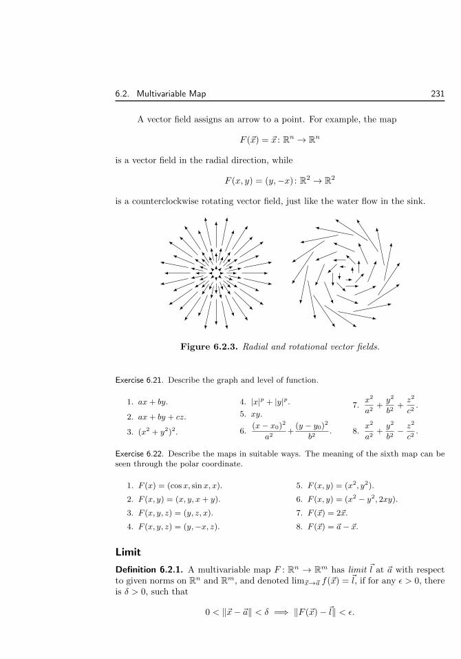
6.2. Multivariable Map 231
A vector field assigns an arrow to a point. For example, the map
F (~x) = ~x : Rn → Rn
is a vector field in the radial direction, while
F (x, y) = (y,−x) : R2 → R2
is a counterclockwise rotating vector field, just like the water flow in the sink.
Figure 6.2.3. Radial and rotational vector fields.
Exercise 6.21. Describe the graph and level of function.
1. ax+ by.
2. ax+ by + cz.
3. (x2 + y2)2.
4. |x|p + |y|p.5. xy.
6.(x− x0)2
a2+
(y − y0)2
b2.
7.x2
a2+y2
b2+z2
c2.
8.x2
a2+y2
b2− z2
c2.
Exercise 6.22. Describe the maps in suitable ways. The meaning of the sixth map can beseen through the polar coordinate.
1. F (x) = (cosx, sinx, x).
2. F (x, y) = (x, y, x+ y).
3. F (x, y, z) = (y, z, x).
4. F (x, y, z) = (y,−x, z).
5. F (x, y) = (x2, y2).
6. F (x, y) = (x2 − y2, 2xy).
7. F (~x) = 2~x.
8. F (~x) = ~a− ~x.
Limit
Definition 6.2.1. A multivariable map F : Rn → Rm has limit ~l at ~a with respectto given norms on Rn and Rm, and denoted lim~x→~a f(~x) = ~l, if for any ε > 0, thereis δ > 0, such that
0 < ‖~x− ~a‖ < δ =⇒ ‖F (~x)−~l‖ < ε.

232 Chapter 6. Multivariable Function
To emphasize that the map is defined on a subset A, we sometimes denote thelimit by lim~x∈A,~x→~a F (~x) = ~l. If B ⊂ A, then by restricting the definition of thelimit from ~x ∈ A to ~x ∈ B, we find
lim~x∈A,~x→~a
F (~x) = ~l =⇒ lim~x∈B,~x→~a
F (~x) = ~l.
In particular, if the restrictions of a map on different subsets give different limits,then the limit diverges. On the other hand, for a finite union, lim~x∈A1∪···∪Ak,~x→~a F (~x)converges if and only if all lim~x∈Ai,~x→~a F (~x) converge and have the same value.
Let fi and li be the coordinates of F and ~l. For the L∞-norm on Rm, it iseasy to see that
lim~x→~a
F (~x) = ~l ⇐⇒ lim~x→~a
fi(~x) = li for all i.
Once we prove all norms are equivalent in Theorem 6.3.8, the property also holdsfor any norm on Rm.
The limit of multivariable maps and functions has most of the usual propertiesenjoyed by single variable functions. The major difference between functions andmaps is that values of functions can be compared, but values of maps cannot becompared. For example, the following extends the similar Propositions 2.1.7 and2.3.3 for single variable functions (k is used because m and n are reserved fordimensions). The same proof applies here.
Proposition 6.2.2. For a map F , lim~x→~a F (~x) = ~l if and only if limn→∞ ~xk = ~a
and ~xk 6= ~a imply limk→∞ F (~xk) = ~l.
We may also define various variations at ∞ by replacing ‖~x − ~a‖ < δ with‖~x‖ > N or replacing |f(~x)− l| < ε by |f(~x)| > b.
Example 6.2.1. Consider f(x, y) =xy(x2 − y2)
x2 + y2defined for (x, y) 6= (0, 0). By |f(x, y)| ≤
|xy|, we have ‖(x, y)‖∞ < δ =√ε implying |f(x, y)| ≤ ε. Therefore limx,y→0 f(x, y) = 0
in the L∞-norm. By the equivalence between the Lp-norms, the limit also holds for otherLp-norms.
Example 6.2.2. Consider f(x, y) =xy
x2 + y2defined for (x, y) 6= (0, 0). We have f(x, cx) =
c
1 + c2, so that limy=cx, (x,y)→(0,0) f(x, y) =
c
1 + c2. Since the restriction of the function
to straight lines of different slopes gives different limits, the function diverges at (0, 0).
Example 6.2.3. For any angle θ ∈ [0, 2π), we choose a number δθ > 0, and define
f(t cos θ, t sin θ) =
0, if |t| < δθ,
1, if |t| ≥ δθ.
We also allow δθ = +∞, for which we have f(t cos θ, t sin θ) = 0 for all t. Then we havea function on R2, such that the limit at (0, 0) along any straight line is 0. On the other
6.2. Multivariable Map 233
hand, by choosing
δθ =
θ, if θ = 1
n,
+∞, otherwise,
the corresponding function diverges at (0, 0).
Example 6.2.4. Let f(x, y) =xpyq
(xm + yn)k, with p, q,m, n, k > 0. We wish to find out
when limx,y→0+ f(x, y) = 0.Let
A = (x, y) : xm ≤ yn, x > 0, y > 0, B = (x, y) : yn ≤ xm, x > 0, y > 0.
Then the limit we want is equivalent to the convergence to 0 when restricted to A and toB. For (x, y) ∈ A, we have yn ≤ xm + yn ≤ 2yn, so that
2−kxpyq−nk =xpyq
(2yn)k≤ xpyq
(xm + yn)k≤ xpyq
(yn)k= xpyq−nk.
Therefore lim(x,y)∈A, x,y→0+ f(x, y) = 0 if and only if lim(x,y)∈A, x,y→0+ xpyq−nk = 0.If we further restrict the limit to A ∩ B = (x, y) : xm = yn, x > 0, y > 0, then
we get the necessary condition limy→0+(ynm )pyq−nk = 0, which means
p
m+q
n> k.
Conversely, we always have 0 ≤ xpyq−nk ≤ (ynm )pyq−nk = yn( pm+ q
n−k) on A. Therefore
lim(x,y)∈A, x,y→0+ xpyq−nk = 0 if and only ifp
m+q
n> k.
By the similar argument, we find lim(x,y)∈B, x,y→0+ f(x, y) = 0 if and only ifp
m+q
n>
k. Thus we conclude that limx,y→0+ f(x, y) = 0 if and only ifp
m+q
n> k.
Exercise 6.23. Find the condition for limx,y→0+ f(x, y) = 0. Assume all the parametersare positive.
1. (xp + yq)r log(xm + yn).
2. xp log
(1
xm+
1
yn
).
3.xpyq
(xm + yn)k(xm′ + yn′)k′.
4.(xp + yq)r
(xm + yn)k.
Exercise 6.24. Compute the convergent limits. All parameters are positive.
1. lim(x,y)→(1,1)1
x− y .
2. limx,y,z→0xyz
x2 + y2 + z2.
3. lim(x,y)→(0,0)(x− y) sin1
x2 + y2.
4. limx,y→∞(x− y) sin1
x2 + y2.
5. limx,y→∞(x2 + y2)p
(x4 + y4)q.
6. lim0<x<y2,x→0,y→0
xpy
x2 + y2.
7. limax≤y≤bx, x,y→∞1
xy.
8. limx,y→0+(x+ y)xy.
9. limx→∞,y→0
(1 +
1
x
) x2
x+y
.
10. limx,y→+∞
(1 +
1
x
) x2
x+y
.
11. limx,y→+∞x2 + y2
ex+y.
234 Chapter 6. Multivariable Function
Exercise 6.25. Show that limx,y→0xy2
x2 + y4diverges, although the limit converges to 0 along
any straight line leading to (0, 0).
Exercise 6.26. Extend Example 6.2.3 to higher dimension. For each vector ~v in the unitsphere S2, choose a number δ~v > 0 and define
f(t~v) =
0, if |t| < δ~v,
1, if |t| ≥ δ~v.
1. Find a sequence of vectors ~vn in S2, such that no three vectors lie in the same2-dimensional plane.
2. Choose δ~vn =1
nand δ~v = +∞ otherwise. Prove that the corresponding f(x, y)
diverges at ~0, yet the restriction of the function to any plane converges to 0.
Exercise 6.27. Suppose f(x) and g(x) are defined on the right side of 0. Find the necessaryand sufficient condition for limx,y→0+ f(x)g(y) to converge.
Exercise 6.28. Suppose f(x) and g(y) are defined near 0. Find the necessary and sufficientcondition for limx,y→0 f(x)g(y) to converge.
Exercise 6.29. Suppose R2 has the L∞-norm. Prove that (f, g) : Rn → R2 is continuous ifand only if both functions f and g are continuous.
Exercise 6.30. Prove Proposition 6.2.2.
Repeated Limit
For multivariable maps, we may first take the limit in some variables and thentake the limit in other variables. In this way, we get repeated limits such aslim~x→~a lim~y→~b F (~x, ~y). The following result tells us the relation between the re-
peated limits and the usual limit lim(~x,~y)→(~a,~b) F (~x, ~y). The proof is given for the
the norm ‖(~x, ~y)‖ = max‖~x‖, ‖~y‖.
Proposition 6.2.3. Suppose F (~x, ~y) is defined near (~a,~b). Suppose
lim(~x,~y)→(~a,~b)
F (~x, ~y) = ~l,
and
lim~y→~b
F (~x, ~y) = G(~x) for each ~x near ~a.
Then
lim~x→~a
lim~y→~b
F (~x, ~y) = lim(~x,~y)→(~a,~b)
F (~x, ~y).

6.2. Multivariable Map 235
Proof. For any ε > 0, there is δ > 0, such that
0 < max‖~x− ~a‖, ‖~y −~b‖ < δ =⇒ ‖F (~x, ~y)−~l‖ < ε.
Then for each fixed ~x near ~a, taking ~y → ~b in the inequality above gives us
0 < ‖~x− ~a‖ < δ =⇒ ‖G(~x)− l‖ = lim~y→~b‖F (~x, ~y)−~l‖ ≤ ε.
This implies that lim~x→~aG(~x) = ~l, and proves the proposition.
Example 6.2.5. For f(x, y) =xy
x2 + y2in Example 6.2.2, we have
limx→0
f(x, y) = 0 for each y, limy→0
f(x, y) = 0 for each x.
Thereforelimy→0
limx→0
f(x, y) = limx→0
limy→0
f(x, y) = 0.
However, the usual limit lim(x,y)→(0,0) f(x, y) diverges.
Exercise 6.31. Study limx→0,y→0, limx→0 limy→0 and limy→0 limx→0. Assume p, q, r > 0.
1.x− y + x2 + y2
x+ y.
2. x sin1
x+ y cos
1
x.
3.|x|p|y|q
(x2 + y2)r.
4.x2y2
|x|3 + |y|3 .
5. (x+ y) sin1
xsin
1
y.
6.ex − ey
sinxy.
Exercise 6.32. Define a concept of the uniform convergence and find the condition forproperties such as lim~x→~a lim~y→~b F (~x, ~y) = lim~y→~b lim~x→~a F (~x, ~y), similar to Theorem5.4.1.
Exercise 6.33. For each of three limits lim(~x,~y)→(~a,~b), lim~x→~a lim~y→~b and lim~y→~b lim~x→~a,construct an example so that the limit converges but the other two limits diverge. More-over, for each limit, construct an example so that the limit diverges but the other twoconverge and are equal.
Continuity
A map F defined on a subset A is continuous at ~a ∈ A if lim~x→~a F (~x) = F (~a). Thismeans that, for any ε > 0, there is δ > 0, such that
‖~x− ~a‖ < δ =⇒ ‖F (~x)− F (~a)‖ < ε.
The map is uniformly continuous on A if for any ε > 0, there is δ > 0, such that
~x, ~y ∈ A, ‖~x− ~y‖ < δ =⇒ ‖F (~x)− F (~y)‖ < ε.
By Proposition 6.2.2, we know that F is continuous at ~a if and only if
limn→∞
~xk = ~a =⇒ limn→∞
F (~xk) = F (~a).

236 Chapter 6. Multivariable Function
The continuity is also equivalent to the continuity of its coordinate functions (ini-tially for L∞-norm, and eventually for all norms after Theorem 6.3.8). Many prop-erties of continuous functions can be extended to maps. For example, the sum andthe composition of continuous maps are still continuous. The scalar product of acontinuous function and a continuous map is a continuous map. The dot productof two continuous maps is a continuous function.
Example 6.2.6. By direct argument, it is easy to see that the product function µ(x, y) =xy : R2 → R is continuous. Suppose f(~x) and g(~x) are continuous. Then F (~x) =(f(~x), g(~x)) : Rn → R2 is also continuous because each coordinate function is continuous.The composition (µ F )(~x) = f(~x)g(~x) of the two continuous maps is also continuous.Therefore we conclude that the product of continuous functions is continuous.
Exercise 6.34. Prove that any norm is a continuous function with respect to itself. Is thenorm a uniformly continuous function?
Exercise 6.35. Prove that F : Rn → Rm is continuous with respect to the L∞-norm on Rmif and only if F · ~a is a continuous function for any ~a ∈ Rm.
Exercise 6.36. Prove that if f(x, y) is monotone and continuous in x and is continuous iny, then f(x, y) is continuous with respect to the L∞-norm.
Exercise 6.37. Find a function f(x, y) that is continuous in x and in y, but is not continuousat a point (x0, y0) as a two variable function. Moreover, show that the two repeated limitslimx→x0 limy→y0 f(x, y) and limy→y0 limx→x0 f(x, y) of such a function exist and are equal,yet the whole limit lim(x,y)→(x0,y0) f(x, y) diverges.
Exercise 6.38. Prove that the addition (~x, ~y) → ~x + ~y : Rn × Rn → Rn and the scalarmultiplication (c, ~x)→ c~x : R× Rn → Rn are continuous.
Exercise 6.39. Prove that if f(~x) and g(~x) are continuous at ~x0, and h(u, v) is continuousat (f(~x0), g(~x0)) with respect to the L∞-norm on R2, then h(f(~x), g(~x)) is continuous at~x0.
Exercise 6.40. Prove that the composition of two continuous maps is continuous. Then useExercise 6.38 to explain that the sum of two continuous maps is continuous. Moreover,please give a theoretical explanation to Exercise 6.39.
Exercise 6.41. Study the continuity.
1.
sinxy
x, if x 6= 0,
0, if x = 0.
2.
y if x is rational,
−y, if x is irrational.
Exercise 6.42. Suppose f(x) and g(y) are functions defined near 0. Find the necessary andsufficient condition for f(x)g(y) to be continuous at (0, 0).
Exercise 6.43. Suppose φ(x) is uniformly continuous. Is f(x, y) = φ(x) uniformly continu-

6.3. Compact Subset 237
ous with respect to the L∞-norm?
Exercise 6.44. A map F (~x) is Lipschitz if ‖F (~x)− F (~y)‖ ≤ L‖~x− ~y‖ for some constant L.Prove that Lipschitz maps are uniformly continuous.
Exercise 6.45. Prove that the sum of uniformly continuous functions is uniformly continu-ous. What about the product?
Exercise 6.46. Prove that a uniformly continuous map on a bounded subset of Rn isbounded.
Exercise 6.47. Prove that lim~x→~a F (~x) converges if and only if it converges along anycontinuous path leading to ~a.
Exercise 6.48. Suppose f(x) has continuous derivative. Prove that
lim(x,y)→(a,a)
f(x)− f(y)
x− y = f ′(a).
What if the continuity condition is dropped? Is there a similar conclusion for the secondorder derivative?
Intermediate Value Theorem
For single variable functions, the Intermediate Value Theorem says that the contin-uous image of any interval is again an interval. So the theorem is critically relatedto the interval. For multivariable functions, the interval may be replaced by pathconnected subset. Recall that a subset A is path connected if for any ~a,~b ∈ A, thereis a continuous map (i.e., a curve) φ : [0, 1]→ A, such that φ(0) = ~a and φ(1) = ~b.
Proposition 6.2.4. Suppose f(~x) is a continuous function on a path connected sub-
set A. Then for any ~a,~b ∈ A and γ between f(~a) and f(~b), there is ~c ∈ A, such thatf(~c) = γ.
Proof. Since A is path connected, there is a continuous curve φ(t) : [0, 1]→ A such
that φ(0) = ~a and φ(1) = ~b. The composition g(t) = f(φ(t)) is then a continuous
function for t ∈ [0, 1]. Since y is between g(0) = f(~a) and g(1) = f(~b), by Theorem2.5.1, there is c ∈ [a, b], such that g(c) = γ. The conclusion is the same as f(~c) = γfor ~c = φ(c).
6.3 Compact SubsetWe wish to extend properties of continuous single variable functions. For example,we will establish the following extension of Theorems 2.4.1 and 2.4.2.
Theorem 6.3.1. A continuous function on a compact subset is bounded, uniformlycontinuous, and reaches its maximum and minimum.

238 Chapter 6. Multivariable Function
Needless to say, the compact subset is the higher dimensional version ofbounded and closed intervals. The concept should be defined by certain proper-ties so that the proofs of Theorems 2.4.1 and 2.4.2 remains valid. The following isthe proof of the boundedness property, paraphrased from the original proof.
Proof. Suppose f is continuous on a compact subset K. If f is not bounded, thenthere is a sequence ~xk ∈ K, such that limk→∞ f(~xk) = ∞. Since K is compact,there is a subsequence ~xkp converging to ~a ∈ K. By the continuity of f(~x) at ~a,this implies that f(~xkp) converges to (~a). Since this contradicts the assumptionlimk→∞ f(~xk) =∞, we conclude that f is actually bounded on K.
Note that the proof is quite formal. It does not refer specifically to the norm,or even vectors in the Euclidean space. The proof actually makes sense in anytopological space. From the analysis viewpoint, topology is the formal theory basedon the formal notion of limits.
Compact Subset
By examining the proof above, we get the following definition of compact subsets.
Definition 6.3.2. A subset of a Euclidean space is compact if any sequence in thesubset has a convergent subsequence, and the limit of the subsequence still lies inthe subset.
As remarked after the proof, a suitable generalization (called net, Moore-Smithsequence, or filter) of the definition is actually the concept of compact subset in anytopological space.
Theorem 6.3.1 can be extended to multivariable maps, with the loss of themaximum and minimum property.
Proposition 6.3.3. A continuous map F on a compact subset K is bounded anduniformly continuous. Moreover, the image subset F (K) = F (~x) : ~x ∈ K is alsocompact.
A subset A ⊂ Rn is bounded (with respect to a norm) if there is a constant B,such that ‖~x‖ < B for any ~x ∈ A.
Proof. The proof of the usual properties of F is the same as before. We only provethe compactness of F (K). A sequence in F (K) is F (~xk), with ~xk ∈ K. Since K iscompact, there is a subsequence ~xkp converging to ~a ∈ K. By the continuity of Fat ~a ∈ K, we have
limk→∞
F (~xkp) = F (~a) ∈ F (K).
Therefore the subsequence F (~xkp) of F (~xk) converges to a limit in F (K).

6.3. Compact Subset 239
Example 6.3.1. Let A = [a, b] ⊂ R be a bounded and closed interval. Then any sequencexk ∈ A is bounded. By Bolzano-Weierstrass Theorem (Theorem 1.5.1), there is a converg-ing subsequence xkp . By a ≤ xkp ≤ b and the order rule, we have a ≤ limxkp ≤ b, whichmeans limxkp ∈ A.
Example 6.3.2. The sequence k−1 ∈ A = k−1 : k ∈ N converges to 0. Therefore anysubsequence k−1
p also converges to 0. This implies that no subsequence converges to alimit in A, and therefore A is not compact.
If we also include the limit 0, then we expect A = A ∪ 0 to be compact. Indeed,any sequence xk ∈ A is one of two kinds. The first is that infinitely many xk are equal.This means that there is a constant subsequence xkp ∈ A, which converges to xk1 ∈ A.The second is that there are infinitely many different xk. For our specific A, this impliesthat there is a subsequence xkp = ξ−1
p ∈ A with ξp → ∞. Then limxkp = 0 ∈ A. Weconclude that A is compact.
Example 6.3.3. Suppose lim ~xk = ~l. Then F (k−1) = ~xk and F (0) = ~l define a mapF : A → Rn from the subset in Example 6.3.2. It is easy to verify that F is continuous.By Theorem 6.3.3, therefore, the image subset F (A) is also compact. Note that F (A) is
the subset of all ~xk together with ~l.
Exercise 6.49. With the help of Exercise 1.44, extend the argument in Example 6.3.1 toprove that any bounded and closed rectangle [a1, b1] × [a2, b2] × · · · × [an, bn] is compactwith respect to the L∞-norm.
Exercise 6.50. Suppose ~xn ∈ A converges to ~l 6∈ A. Prove that A is not compact.
Exercise 6.51. Directly prove that the subset of all ~xn together with ~l in Example 6.3.3 isa compact subset.
Exercise 6.52. Suppose K is a compact subset. Prove that there are ~a,~b ∈ K, such that‖~a−~b‖ = max~x,~y∈K ‖~x− ~y‖.
Exercise 6.53. Prove that the union of two compact subsets is compact.
Exercise 6.54. Using the product norm in Exercise 6.4, prove that if K,L are compact,then K × L is compact. Conversely, if K,L 6= ∅ and K × L is compact, then K,L arecompact.
Exercise 6.55. Prove the uniform continuity of a continuous map on a compact subset.
Exercise 6.56. Prove that a continuous function on a compact subset reaches its maximumand minimum. What is the meaning of the fact for the compact subset A in Example6.3.2?
Inverse Map
We cannot talk about multivariable monotone maps. Thus the only part of Theorem2.5.3 that can be extended is the continuity.
240 Chapter 6. Multivariable Function
Proposition 6.3.4. Suppose F : K ⊂ Rn → Rm is a one-to-one and continuousmap on a compact subset K. Then the inverse map F−1 : F (K) ⊂ Rm → Rn isalso continuous.
Proof. We claim that F−1 is in fact uniformly continuous. Suppose it is not uni-formly continuous. Then there is ε > 0 and ~ξk = F (~xk), ~ηk = F (~yk) ∈ F (K), suchthat
limk→∞
‖~ξk − ~ηk‖ = 0, ‖~xk − ~yk‖ = ‖F−1(~ξk)− F−1(~ηk)‖ ≥ ε.
By the compactness of K, we can find kp, such that both limp→∞ ~xkp = ~a and
limp→∞ ~ykp = ~b converge, and both ~a and ~b lie in K. Then by the continuity of F
at ~a and ~b, we have
limp→∞
~ξkp = limp→∞
F (~xkp) = F (~a), limp→∞
~ηkp = limp→∞
F (~ykp) = F (~b).
We conclude that ‖F (~a) − F (~b)‖ = limp→∞ ‖~ξkp − ~ηkp‖ = 0, so that F (~a) = F (~b).
Since F is one-to-one, we get ~a = ~b. This contradicts with limp→∞ ~xkp = ~a,
limp→∞ ~ykp = ~b, and ‖~xk − ~yk‖ ≥ ε.
Closed Subset
The concept of compact subsets is introduced as a high dimensional substitute ofbounded and closed intervals. So we expect the compactness to be closely relatedto the high dimensional version of bounded and closed subsets.
By applying Bolzano-Weierstrass Theorem to each coordinate (see Exercise1.44), we find that any sequence in a bounded subset K has a convergent subse-quence (with respect to the L∞-norm). For K to be compact, therefore, it remainsto satisfy the following
~xk ∈ K, limk→∞
~xk = ~l =⇒ ~l ∈ K.
Definition 6.3.5. A subset of a Euclidean space is closed if the limit of any conver-gent sequence in the subset still lies in the subset.
Proposition 6.3.6. A subset of the Euclidean space is compact if and only if it isbounded and closed.
Proof. For the special case of the L∞-norm, we have argued that bounded andclosed subsets are compact. The converse will be proved for any norm.
Suppose K is not bounded. Then there is a sequence ~xk ∈ K satisfyinglimk→∞ ‖~xk‖ =∞. This implies that limk→∞ ‖~xkp‖ =∞ for any subsequence ~xkp .By Exercise 6.11, ~xkp must diverge. This shows that K is not compact.
Suppose K is not closed. Then there is a convergent sequence ~xk ∈ K withlimk→∞ ~xk = ~l 6∈ K. Therefore any subsequence ~xkp converges to ~l 6∈ K, so that nosubsequence has limit in K. This shows that K is not compact.

6.3. Compact Subset 241
Proposition 6.3.7. Closed subsets have the following properties.
1. ∅ and Rn are closed.
2. Intersections of closed subsets are closed.
3. Finite unions of closed subsets are closed.
Proof. The first property is trivially true.Suppose Ci are closed and C = ∩Ci. Suppose ~xk ∈ C and limk→∞ ~xk = ~l.
Then the sequence ~xk lies in each Ci. Because Ci is closed, the limit ~l lies in eachCi. Therefore ~l ∈ ∩Ci = C.
Suppose C and D are closed. Suppose ~xk ∈ C ∪D and limk→∞ ~xk = ~l. Thenthere must be infinitely many ~xk in either C or D. In other words, there is asubsequence in either C or D. If C contains a subsequence ~xkp , then because C
is closed, we get ~l = limk→∞ ~xk = limp→∞ ~xkp ∈ C. If D contains a subsequence,
then we similarly get ~l ∈ D. Therefore ~l ∈ C ∪D.
Example 6.3.4. Any closed interval [a, b] is a closed subset of R. The reason is the orderrule. Suppose xk ∈ [a, b] and limxk = l. By a ≤ xk ≤ b and the order rule, we havea ≤ l ≤ b, which means l ∈ [a, b].
Exercise 6.57. Prove that if two norms are equivalent, then a subset is bounded, compact,or closed with respect to one norm if and only if it has the same property with respect tothe other norm.
Exercise 6.58. Prove that any closed rectangle [a1, b1] × [a2, b2] × · · · × [an, bn] is a closedsubset of Rn with respect to the L∞-norm.
Exercise 6.59. Prove that both the closed ball B(~x, r) = ~x : ‖~x‖ ≤ r and the sphereS(~x, r) = ~x : ‖~x‖ = r are bounded and closed. Moreover, for the L∞-norm, prove thatboth B(~x, r) and S(~x, r) are compact.
Exercise 6.60. Using the product norm in Exercise 6.4, prove that if A,B are closed, thenA×B is closed. Conversely, if A,B 6= ∅ and A×B is closed, then A,B are closed.
Exercise 6.61. Suppose K is compact and C is closed. Prove that if C ⊂ K, then C is alsocompact.
Exercise 6.62. Suppose ~xk is a sequence with no converging subsequence. Prove that thesubset of all ~xk is closed.
Exercise 6.63. Theorem 6.3.3 tells us the image of a bounded closed subset under a con-tinuous map is still bounded and closed. Show that the image of a closed subset under acontinuous map is not necessarily closed.
Exercise 6.64. A collection of subsets Ai is locally finite if for any ~x ∈ Rn, there is ε > 0,such that Ai ∩ B(~x, ε) = ∅ for all but finitely many Ai. Prove that the union of a locally
242 Chapter 6. Multivariable Function
finite collection of closed subsets is also closed.
Exercise 6.65. For any subset A of Rn, the closure of A is (compare with the definition ofLIMxk in Section 1.5)
A =
limk→∞
~xk : ~xk ∈ A and limk→∞
~xk converges.
Prove that the closure is closed (compare with Exercise 1.47).
Exercise 6.66. Prove that the closure A is the smallest closed subset containing A, and Ais closed if and only if A = A.
Equivalence of Norms
The following result allows us to freely use any norm in multivariable analysis.
Theorem 6.3.8. All norms on a finite dimensional vector space are equivalent.
Proof. We prove the claim for norms on a Euclidean space. Since linear algebratells us that any finite dimensional vector space is isomorphic to a Euclidean space,the result applies to any finite dimensional vector space.
We compare any norm ‖~x‖ with the L∞-norm ‖~x‖∞. Let ~e1 = (1, 0, . . . , 0),~e2 = (0, 1, . . . , 0), . . . , ~en = (0, 0, . . . , 1) be the standard basis of Rn. By thedefinition of norm, we have
‖~x‖ = ‖x1~e1 + x2~e2 + · · ·+ xn~en‖≤ |x1|‖~e1‖+ |x2|‖~e2‖+ · · ·+ |xn|‖~en‖≤ (‖~e1‖+ ‖~e2‖+ · · ·+ ‖~en‖) max|x1|, |x2|, . . . , |xn|= (‖~e1‖+ ‖~e2‖+ · · ·+ ‖~en‖)‖~x‖∞ = c1‖~x‖∞.
It remains to prove that ‖x‖ ≥ c2‖~x‖∞ for some c2 > 0. A special case is
‖~x‖∞ = 1 =⇒ ‖~x‖ ≥ c2.
Conversely, given the special case, we write any vector ~x as ~x = r~u with r = ‖~x‖∞and ‖~u‖∞ = 1 (see Exercise 6.5). Then we get the general case
‖~x‖ = ‖r~u‖ = r‖~u‖ ≥ rc2 = c2‖~x‖∞.
Therefore it is sufficient to prove the special case.We interpret the special case as the norm function ‖~x‖ having a positive
minimum on the subset K = ~x : ‖~x‖∞ = 1. We know that K is bounded andclosed with respect to the L∞-norm, so by Proposition 6.3.6 (fully proved for theL∞-norm), K is compact with respect to the L∞-norm (see Exercise 6.59). On theother hand, the inequality |‖~x‖ − ‖~y‖| ≤ ‖~x − ~y‖ ≤ c1‖~x − ~y‖∞ implies that thenorm function ‖~x‖ is continuous with respect to the L∞-norm. Then by Theorem6.3.1, the norm ‖~x‖ reaches its minimum on K at some ~a ∈ K. The minimum value‖~a‖ (to be taken as c2) is positive because
~a ∈ K =⇒ ‖~a‖∞ = 1 =⇒ ~a 6= ~0 =⇒ ‖~a‖ > 0.

6.4. Open Subset 243
6.4 Open Subset
Open Subset
In the analysis of single variable functions, such as differentiability, we often requirefunctions to be defined at all the points near a given point. For multivariablefunctions, the requirement becomes the following concept.
Definition 6.4.1. A subset of a Euclidean space is open if for any point in the subset,all the points near the point are also in the subset.
Thus a subset U is open if
~a ∈ U =⇒ B(~a, ε) ⊂ U for some ε > 0.
U
~a
U
~a
Figure 6.4.1. Definition of open subset.
Exercise 6.67. Prove that if two norms are equivalent, then a subset is open with respectto one norm if and only if it is open with respect to the other norm.
Exercise 6.68. Using the product norm in Exercise 6.4, prove that if A,B are open, thenA×B is open. Conversely, if A,B 6= ∅ and A×B is open, then A,B are open.
Exercise 6.69. The characteristic function of a subset A ⊂ Rn is
χA(~x) =
1, if ~x ∈ A,0, if ~x 6∈ A.
Prove that χA is continuous at ~a if and only if some ball around ~a is either contained inA or is disjoint from A.
Exercise 6.70. For a continuous function f on R, prove that the subset (x, y) : y < f(x)is open. What if f is not continuous?
Closed subsets are defined by using sequence limit. The following is the inter-pretation of open subsets by sequence limit.
Proposition 6.4.2. A subset U of Euclidean space is open if and only if for anysequence ~xk converging to a limit in U , we have ~xk ∈ U for sufficiently large k.

244 Chapter 6. Multivariable Function
Proof. Suppose U is open and limk→∞ ~xk = ~a ∈ U . Then by the definition of Uopen, a ball B(~a, ε) is contained in U . Moreover, by the definition of sequence limit,we have ‖~xk − ~a‖ < ε for sufficiently large k. Then we get ~xk ∈ B(~a, ε) ⊂ U forsufficiently large k.
Suppose U is not open. Then there is ~a, such that B(~a, ε) is never contained
in U . By taking ε =1
k, we get a sequence ~xk /∈ U satisfying ‖~xk − ~a‖ <
1
k. The
sequence converges to ~a ∈ U but completely lies outside U . The contradictionproves the converse.
Now we can use the sequence limit to argue the following property.
Proposition 6.4.3. A subset U of Rn is open if and only if the complement Rn−Uis closed.
Proof. Suppose U be open. To prove that the complement C = Rn − U is closed,we assume that a sequence ~xk ∈ C converges to ~a and wish to prove ~a ∈ C. If~a /∈ C, then ~a ∈ U . By ~xk converging to ~a and Proposition 6.4.2, this implies that~xk ∈ U for sufficiently large k. Since this contradicts to the assumption ~xk ∈ C, weconclude that ~a ∈ C.
Suppose C is closed. To prove that the complement C = Rn − U is open,we assume that a sequence ~xk converges to ~a ∈ U and (by Proposition 6.4.2) wishto prove ~xk ∈ U for sufficiently large k. If our wish is wrong, then there is asubsequence ~xkp /∈ U . Since ~xk converges to ~a, the subsequence also converges to~a. Since ~xkp /∈ U means ~xkp ∈ C, by C closed, the limit ~a of the subsequence mustalso lie in C. This contradicts to the assumption ~a ∈ U . Therefore we must have~xk ∈ U for sufficiently large k.
Combining Propositions 6.3.7 and 6.4.3 gives properties of open subsets.
Proposition 6.4.4. Open subsets have the following properties.
1. ∅ and Rn are open.
2. Unions of open subsets are open.
3. Finite intersections of open subsets are open.
The three properties can be used as the axiom of general topology theory.
Exercise 6.71. Prove Proposition 6.4.4 by directly using the definition of open subsets.
Exercise 6.72. Prove Proposition 6.4.4 by using the sequence limit characterisation of opensubsets in Proposition 6.4.2.
The following describes the relation between open subsets and balls.

6.4. Open Subset 245
Proposition 6.4.5. A subset is open if and only if it is a union of balls. In fact, wecan choose the union to be countable.
Proof. First we prove that any ball B(~a, ε) is open. If ~x ∈ B(~a, ε), then ‖~x−~a‖ < ε.For δ = ε− ‖~x− ~a‖ > 0, we have B(~x, δ) ⊂ B(~a, ε) by
~y ∈ B(~x, δ) =⇒ ‖~y − ~a‖ ≤ ‖~y − ~x‖+ ‖~x− ~a‖ < δ + ‖~x− ~a‖ = ε.
This proves that B(~a, ε) is open.Since balls are open, by the second property in Proposition 6.4.4, the unions
of balls are also open. Conversely, suppose U is open, then for any ~a ∈ U , we havea ball B(~a, ε~a) ⊂ U , where the radius ε~a may depend on the point. Then
U ⊂ ∪~a∈U~a ⊂ ∪~a∈UB(~a, ε~a) ⊂ U
shows that U = ∪~a∈UB(~a, ε~a) is a union of balls.To express U as a union of countably many balls, we use the fact that any
vector has arbitrarily close rational vectors nearby. The fact can be directly verifiedfor Lp-norms, and the general case will follow from Theorem 6.3.8. For each ~a ∈ U ,we have B(~a, ε~a) ⊂ U . By choosing smaller ε~a if necessary, we may further assume
that ε~a is rational. Pick a rational vector ~r~a ∈ Qn satisfying d(~r~a,~a) <ε~a2
. Then
we have ~a ∈ B(~r~a,
ε~a2
)⊂ B(~a, ε~a). The same argument as before gives us
U = ∪~a∈UB(~r~a,
ε~a2
).
Since the collection of all balls with rational center and rational radius is countable,the union on the right is actually countable (after deleting the duplicates).
Exercise 6.73. For any subset A ⊂ Rn and ε > 0, prove that the ε-neighborhood
Aε = ~x : ‖~x− ~a‖ < ε for some ~a ∈ A
is open. Moreover, prove that ∩ε>0Aε = A if and only if A is closed.
Exercise 6.74. For any subset A ⊂ Rn, prove that the interior of A
A = ~x : B(~x, ε) ⊂ A for some ε > 0
is open.
Exercise 6.75. Prove that the interior A is the biggest open subset contained in A, andA = Rn − Rn −A.
Open Subsets in RTheorem 6.4.6. Any open subsets of R is a disjoint union of countably many openintervals. Moreover, the decomposition is unique.

246 Chapter 6. Multivariable Function
Proof. Let U ⊂ R be open. If U = t(ai, bi), then it is easy to see that (ai, bi) aremaximal open intervals in the sense that if (ai, bi) ⊂ (a, b) ⊂ U , then (ai, bi) = (a, b).This already explains the uniqueness of the decomposition.
Since the union of two intervals sharing a point is still an interval, it is easy tosee that any two maximal open intervals must be either identical or disjoint. The(disjoint) union of maximal open intervals is contained in U . It remains to showthat any point x ∈ U also lies in a maximal open interval. In fact, this maximalinterval should be
(ax, bx) = ∪(a, b) : x ∈ (a, b) ⊂ U,
where ax = infa : x ∈ (a, b) ⊂ U and b is the similar supremum. First, thecollection on the right is not empty because U is open. Therefore (ax, bx) is defined.Moreover, if (ax, bx) ⊂ (a, b) ⊂ U , then x ∈ (a, b), so that (a, b) belongs to thecollection on the right. Therefore (a, b) ⊂ (ax, bx). This proves that (ax, bx) ismaximal.
So we have proved that U = t(ai, bi), where (ai, bi) are all the maximal openintervals in U . For any m ∈ N and ε > 0, by maximal open intervals being disjoint,the number of maximal open intervals in U that are contained in (−m,m) and have
length bi − ai ≥1
nis ≤ 2mn. Therefore the collection
(ai, bi) : bi − ai ≥1
n, (ai, bi) ⊂ (−m,m)
is finite. Since any bounded (ai, bi) is contained in some (−m,m) and satisfies
bi − ai ≥1
nfor some n ∈ N, we conclude that the countable collection
∪m,n∈N
(ai, bi) : bi − ai ≥1
n, (ai, bi) ⊂ (−m,m)
is all the bounded maximal open intervals in U . The disjoint property implies thatU has at most two unbounded maximal open intervals. Therefore the number ofmaximal open intervals in U is still countable.
Heine-Borel Theorem
Theorem 6.4.7. Suppose K is a compact subset. Suppose Ui is a collection ofopen subsets such that K ⊂ ∪Ui. Then K ⊂ Ui1 ∪ Ui2 ∪ · · · ∪ Uik for finitely manyopen subsets in the collection.
The single variable version of the theorem is given by Theorem 1.5.6. Forthe L∞-norm, the original proof can be easily adopted to the multivariable ver-sion. The compact subset K is contained in a bounded rectangle I = [α1, β1] ×
[α2, β2]× · · ·× [αn, βn]. By replacing each interval [αi, βi] with either
[αi,
αi + βi2
]or
[αi + βi
2, βi
], the rectangle can be divided into 2n rectangles. If K cannot be
6.4. Open Subset 247
covered by finitely many open subsets from Ui, then for one of the 2n rectangles,denoted I1, the intersection K1 = K ∩ I1 cannot be covered by finitely many opensubsets from Ui. The rest of the construction and the argument can proceed asbefore.
The property in Theorem 6.4.7 is actually the official definition of compactnessin general topological spaces. Therefore the property should imply our definition ofcompactness in terms of the sequence limit.
Exercise 6.76. Suppose K satisfies the property in Theorem 6.4.7. Use the open coverUn = B(~0, n) to prove that K is bounded.
Exercise 6.77. Suppose ~xn ∈ K converges to ~l 6∈ K. Use the open cover Un = Rn−B(~l, n−1)
(complements of closed balls around ~l) to prove that K does not have the property inTheorem 6.4.7.
Exercise 6.78. Prove the converse of Theorem 6.4.7.
Set Theoretical Interpretation of Continuity
Let f : X → Y be a map. Then the image of a subset A ⊂ X is
f(A) = f(x) : x ∈ A ⊂ Y,
and the preimage of a subset B ⊂ Y is
f−1(B) = x ∈ X : f(x) ∈ B ⊂ X.
It is easy to verify that the following properties.
• A ⊂ f−1(B) ⇐⇒ f(A) ⊂ B.
• f−1(f(A)) ⊂ A, f(f−1(B)) = B ∩ f(X).
• A ⊂ A′ =⇒ f(A) ⊂ f(A′).
• B ⊂ B′ =⇒ f−1(B) ⊂ f−1(B′) and f−1(B′ −B) = f−1(B′)− f−1(B).
• f−1(Y −B) = X − f−1(B).
• f(∪Ai) = ∪f(Ai), f(∩Ai) ⊂ ∩f(Ai).
• f−1(∪Bi) = ∪f−1(Bi), f−1(∩Bi) = ∩f−1(Bi).
• (g f)(A) = g(f(A)), (g f)−1(B) = f−1(g−1(A)).
Proposition 6.4.8. For a map F : Rn → Rm, the following are equivalent.
1. F is continuous.
2. The preimage F−1(U) of any open U is open.

248 Chapter 6. Multivariable Function
3. The preimage F−1(B(~b, ε)) of any ball is open.
4. The preimage F−1(C) of any closed C is closed.
If F is defined on a subset A ⊂ Rn, then F−1(B) is open (closed) means thatF−1(B) = A ∩D for a open (closed) subset D ⊂ Rn.
Proof. Suppose F is continuous and U is open. Then for any ~a ∈ F−1(U), we haveF (~a) ∈ U . Since U is open, we have B(F (~a), ε) ⊂ U for some ε > 0. The continuityof F at ~a means that, for this ε, there is δ > 0, such that
‖~x− ~a‖ < δ =⇒ ‖F (~x)− F (~a)‖ < ε.
The implication is the same as
~x ∈ B(~a, δ) =⇒ F (~x) ∈ B(F (~a), ε).
Since B(F (~a), ε) ⊂ U , this tells us F (B(~a, δ)) ⊂ U , which is the same as B(~a, δ) ⊂F−1(U). Thus we have shown that
~a ∈ F−1(U) =⇒ B(~a, δ) ⊂ F−1(U) for some δ > 0.
This proves that F−1(U) is open. So the first statement implies the second.By Proposition 6.4.5, any ball is open. Therefore the third statement is a
special case of the second statement.Now we prove the third statement implies the first. For any ~a and ε > 0,
the third statement says that F−1(B(F (~a), ε)) is open. On the other hand, F (~a) ∈B(F (~a), ε) implies ~a ∈ F−1(B(F (~a), ε)). Therefore the openness implies B(~a, δ) ⊂F−1(B(F (~a), ε)) for some δ > 0. The meaning of the inclusion is exactly
‖~x− ~a‖ < δ =⇒ ‖F (~x)− F (~a)‖ < ε.
This is the first statement.It remains to show that the second and the fourth statements are equivalent.
This follows from Proposition 6.4.3 and the property F−1(Rm−B) = Rn−F−1(B).Suppose the second statement is true. Then for any closed B, the complementRm −B is open. The second statement tells us that the preimage F−1(Rm −B) isalso open. Then F−1(Rm−B) = Rn−F−1(B) tells us that F−1(B) is closed. Theprove that the fourth statement implies the second is the same.
Exercise 6.79. Use Proposition 6.2.2 to give a direct proof that a map F defined on thewhole Euclidean space is continuous if and only if the preimage of any closed subset isclosed.
Exercise 6.80. Prove the following are equivalent for a map F defined on the whole Eu-clidean space. For the definition of closure, see Exercise 6.65.
1. The map is continuous.
2. F (A) ⊂ F (A) for any subset A.
3. F−1(B) ⊃ F−1(B) for any subset B.

6.5. Additional Exercise 249
6.5 Additional ExerciseTopology in a Subset of Rn
The discussion about the open and closed subsets of Rn can be extended to open andclosed relative to a subset X of Rn.
Exercise 6.81. We say a subset A ⊂ X is closed in X (or with respect to X) if
~xn ∈ A, limn→∞
~xn = ~l ∈ X =⇒ ~l ∈ A.
Prove that this happens if and only if A = X ∩ C for a closed subset C of Rn.
Exercise 6.82. We say a subset A ⊂ X is open in X (or with respect to X) if
~x ∈ A =⇒ B(~x, ε) ∩X ⊂ A for some ε > 0.
In other words, for any point in A, all the points of X that are sufficiently near the pointare also in A. Prove that this happens if and only if A = X ∩ U for an open subset U ofRn.
Exercise 6.83. For A ⊂ X ⊂ Rn, prove that A is open in X if and only if X − A is closedin X.
Exercise 6.84. Extend Propositions 6.3.7 and 6.4.4 to subsets of X ⊂ Rn.
Repeated Extreme
Exercise 6.85. For a function f(~x, ~y) on A×B. Prove that
inf~y∈B
sup~x∈A
f(~x, ~y) ≥ sup~x∈A
inf~y∈B
f(~x, ~y) ≥ inf~x∈A
inf~y∈B
f(~x, ~y) = inf~x∈A,~y∈B
f(~x, ~y).
Exercise 6.86. For any a ≥ b1 ≥ c1 ≥ d and a ≥ b2 ≥ c2 ≥ d, can you construct a functionf(x, y) on [0, 1]× [0, 1] such that
sup~x∈A,~y∈B
f = a, inf~y∈B
sup~x∈A
f = b1, inf~x∈A
sup~y∈B
f = b2,
inf~x∈A,~y∈B
f = d, sup~x∈A
inf~y∈B
f = c1, sup~y∈B
inf~x∈A
f = c2.
Exercise 6.87. Suppose f(x, y) is a function on [0, 1] × [0, 1]. Prove that if f(x, y) is in-creasing in x, then infy∈[0,1] supx∈[0,1] f(x, y) = supx∈[0,1] infy∈[0,1] f(x, y). Can the interval[0, 1] be changed to (0, 1)?
Exercise 6.88. Extend the discussion to three or more repeated extrema. For example, canyou give a simple criterion for comparing two strings of repeated extrema?
Homogeneous and Weighted Homogeneous Function
A function f(~x) is homogeneous of degree p if f(c~x) = cpf(~x) for any c > 0. More generally,a function is weighted homogeneous if
cf(x1, x2, . . . , xn) = f(cq1x1, cq2x2, . . . , c
qnxn).
250 Chapter 6. Multivariable Function
The later part of the proof of Theorem 6.3.8 makes use of the fact that any norm is ahomogeneous function of degree 1 (also see Exercise 6.91).
Exercise 6.89. Prove that two homogeneous functions of the same degree are equal awayfrom ~0 if and only if their restrictions on the unit sphere Sn−1 are equal.
Exercise 6.90. Prove that a homogeneous function is bigger than another homogeneousfunction of the same degree away from ~0 if and only if the inequality holds on Sn−1.
Exercise 6.91. Suppose f(~x) is a continuous homogeneous function of degree p satisfyingf(~x) > 0 for ~x 6= ~0. Prove that there is c > 0, such that f(~x) ≥ c‖~x‖p for any ~x.
Exercise 6.92. Prove that a homogeneous function is continuous away from ~0 if and only ifits restriction on Sn−1 is continuous. Then find the condition for a homogeneous functionto be continuous at ~0.
Continuous Map and Function on Compact Set
Exercise 6.93. Suppose F (~x, ~y) is a continuous map on A ×K ⊂ Rm × Rn. Prove that ifK is compact, then for any ~a ∈ A and ε > 0, there is δ > 0, such that ~x ∈ A, ~y ∈ K, and‖~x− ~a‖ < δ imply ‖F (~x, ~y)− F (~a, ~y)‖ < ε.
Exercise 6.94. Suppose f(~x, ~y) is a continuous function on A × K. Prove that if K iscompact, then g(~x) = max~y∈K f(~x, ~y) is a continuous function on A.
Exercise 6.95. Suppose f(~x, y) is a continuous function on A × [0, 1]. Prove that g(~x) =∫ 1
0
f(~x, y)dy is a continuous function on A.
Continuity in Coordinates
A function f(~x, ~y) is continuous in ~x if lim~x→~a f(~x, ~y) = f(~a, ~y). It is uniformly continuousin ~x if the limit is uniform in ~y: For any ε > 0, there is δ > 0, such that ‖~x − ~x′‖ < δimplies ‖F (~x, ~y)− F (~x′, ~y)‖ ≤ ε for any ~y.
Exercise 6.96. Prove that if f(~x, ~y) is continuous, then f(~x, ~y) is continuous in ~x. Moreover,show that the function
f(x, y) =
xy
x2 + y2, if (x, y) 6= (0, 0),
0, if (x, y) = (0, 0),
is continuous in both x and y, but is not a continuous function.
Exercise 6.97. Prove that if f(~x, ~y) is continuous in ~x and is uniformly continuous in ~y,then f(~x, ~y) is continuous.
Exercise 6.98. Suppose f(~x, y) is continuous in ~x and in y. Prove that if f(~x, y) is monotonein y, then f(~x, y) is continuous.

Chapter 7
Multivariable Algebra
251

252 Chapter 7. Multivariable Algebra
7.1 Linear TransformA vector space is a set in which addition ~v + ~w and scalar multiplication c~v aredefined and satisfy the usual properties. A map L : V → W between vector spacesis a linear transform if it preserves the two operations
L(~x+ ~y) = L(~x) + L(~y), L(c~x) = cL(~x).
This implies that the linear combinations are also preserved
L(c1~x1 + c2~x2 + · · ·+ ck~xk) = c1L(~x1) + c2L(~x2) + · · ·+ ckL(~xk).
An isomorphism of vector spaces is an invertible linear transform.Vector space is the natural generalization of the Euclidean space Rn. In fact,
a vector space will always be finite dimensional in this book, and any finite dimen-sional vector space is isomorphic to a Euclidean space.
The linear functions used in the differentiation of single variable functionswill become maps of the form ~a + L(∆~x) in the differentiation of multivariablefunctions. We will call such maps linear maps (more properly named affine maps)to distinguish from linear transforms (for which ~a = ~0).
Matrix of Linear Transform
An ordered collection of vectors α = ~v1, ~v2, . . . , ~vn is a basis of V if any vectorhas unique expression
~x = x1~v1 + x2~v2 + · · ·+ xn~vn.
The coefficient xi is the i-th coordinate of ~x with respect to the basis. Suppose αand β = ~w1, ~w2, . . . , ~wm are ordered basis of V and W . Then a linear transformL : V →W is determined by its values on the basis vectors
L(~v1) = a11 ~w1 + a21 ~w2 + · · ·+ am1 ~wm,
L(~v2) = a12 ~w1 + a22 ~w2 + · · ·+ am2 ~wm,
...
L(~vn) = a1n ~w1 + a2n ~w2 + · · ·+ amn ~wm.
The matrix of L with respect to the (ordered) bases α and β is the transpose of thecoefficients (also see Exercise 7.1)
Lβα =
a11 a12 · · · a1n
a21 a22 · · · a2n
......
...am1 am2 · · · amn
.
The relation between a linear transform and its matrix can be expressed as
Lα = L(~v1 ~v2 · · · ~vn) = (~w1 ~w2 · · · ~wm)Lβα = βLβα.

7.1. Linear Transform 253
Here the left means applying L to each vector, and the right means the “matrixproduct” with ~wi viewed as columns.
The standard basis ε = ~e1, ~e2, . . . , ~en for the Euclidean space Rn is given by
~e1 = (1, 0, . . . , 0), ~e2 = (0, 1, . . . , 0), . . . , ~en = (0, 0, . . . , 1).
The standard matrix for a linear transform L : Rn → Rm is (the two ε may bedifferent)
Lεε = (L(~e1) L(~e2) · · · L(~en)).
Here the vectors L(~e1) ∈ Rm are written vertically and become the columns of thematrix. We may define the addition, scalar multiplication, and product of matricesas corresponding to the addition, scalar multiplication, and composition of lineartransforms between Euclidean spaces.
Exercise 7.1. Suppose L : V → W is a linear transform. Suppose α and β are bases of Vand W , and
~x = x1~v1 + x2~v2 + · · ·+ xn~vn, L(~x) = y1 ~w1 + y2 ~w2 + · · ·+ yn ~wn.
Prove that y1
y2
...ym
=
a11 a12 · · · a1n
a21 a22 · · · a2n
......
...am1 am2 · · · amn
x1
x2
...xn
,
where the matrix is the matrix Lβα of the linear transform.
Exercise 7.2. Suppose K,L : V → W are linear transforms and c is a number. Prove thatthe maps
(K + L)(~x) = K(~x) + L(~x), (cL)(~x) = c(L(~x))
are linear transforms, and their matrices are (K + L)βα = Kβα + Lβα, (cK)βα = cKβα.
Exercise 7.3. Suppose L : U → V and K : V → W are linear transforms. Prove that thecomposition K L : U →W is a linear transform, and its matrix is (K L)γα = KγβLβα.
Exercise 7.4. Suppose L : V →W is an invertible linear transform. Prove that L−1 : W →V is also a linear transform, and (L−1)αβ = (Lβα)−1.
Exercise 7.5. Prove that the sum and scalar multiplication of linear transforms from V toW defined in Exercise 7.2 make the collection Hom(V,W ) of all linear transforms from Vto W into a vector space. Then prove the following.
1. Prove that (c1K1 + c2K2) L = c1K1 L+ c2K2 L. Then explain that for a lineartransform L : U → V , the map
L : Hom(V,W )→ Hom(U,W ).
is a linear transform.

254 Chapter 7. Multivariable Algebra
2. For a linear transform K : V →W , prove that the map
K : Hom(U, V )→ Hom(U,W ).
is a linear transform.
Exercise 7.6. Prove that a linear transform L is injective if and only if K L = I for somelinear transform K. Moreover, L is surjective if and only if L K = I for some lineartransform K.
Change of Basis
Let α and β be two bases of V . We can express the first basis in terms of the secondbases
~v1 = p11 ~w1 + p21 ~w2 + · · ·+ pn1 ~wn,
~v2 = p12 ~w1 + p22 ~w2 + · · ·+ pn2 ~wn,
...
~vn = p1n ~w1 + p2n ~w2 + · · ·+ pnn ~wn.
By viewing the left side as the identity linear transform applied to the first basis,the coefficient matrix
Iβα =
p11 p12 · · · p1n
p21 p22 · · · p2n
......
...pn1 pn2 · · · pnn
is the matrix of the identity transform I : V → V with respect to the bases α (offirst V ) and β (of second V ). This is the usual matrix for changing the basis fromα to β. The matrix is also characterized by
α = βIβα.
Suppose L : V → W is a linear transform. Suppose α, α′ are bases of V , andβ, β′ are bases of W . Then we have
Lα′ = LαIαα′ = βLβαIαα′ = β′Iβ′βLβαIαα′ .
This gives the change of basis formula
Lβ′α′ = Iβ′βLβαIαα′ .
Exercise 7.7. A linear transform L : V → V from a vector space to itself is an endomor-phism. We usually take α = β in this case and say that Lαα is the matrix of L with respectto α. Prove that the matrices A and B of an endomorphism L : V → V with respect todifferent bases of V are similar in the sense that B = PAP−1 for an invertible P .

7.1. Linear Transform 255
Dual Space
A linear functional on a vector space V is a numerical valued linear transforml : V → R. Since the addition and scalar multiplication of linear functionals arestill linear (see Exercises 7.2 and 7.5), all the linear functionals on V form a vectorspace V ∗, called the dual space of V . A linear transform L : V → W induces thedual transform in the opposite direction by simply sending l ∈W ∗ to l L ∈ V ∗
L∗ : V ∗ ←W ∗, L∗(l)(~x) = l(L(~x)).
Given a basis α = ~v1, ~v2, . . . , ~vn of V , we may construct a dual basis α∗ =~v ∗1 , ~v ∗2 , . . . , ~v ∗n of V ∗ by taking ~v ∗i to be the i-th coordinate with respect to thebasis α
~x = x1~v1 + x2~v2 + · · ·+ xn~vn 7→ ~v ∗i (~x) = xi.
In other words, the dual basis is characterized by
~x = ~v ∗1 (~x)~v1 + ~v ∗2 (~x)~v2 + · · ·+ ~v ∗n (~x)~vn.
Moreover, α∗ is indeed a basis of V ∗ because any linear functional l has uniquelinear expression
l = a1~v∗1 + a2~v
∗2 + · · ·+ an~v
∗n , ai = l(~vi),
orl = l(~v1)~v ∗1 + l(~v2)~v ∗2 + · · ·+ l(~vn)~v ∗n .
Proposition 7.1.1. Suppose V is a finite dimensional vector space. Then
~x 7→ ~x∗∗, ~x∗∗(l) = l(~x)
is an isomorphism V ∼= (V ∗)∗.
Proof. The following shows that ~x∗∗ is indeed a linear functional on V ∗ and thereforebelongs to the double dual (V ∗)∗
~x∗∗(c1l1 + c2l2) = (c1l1 + c2l2)(~x) = c1l1(~x) + c2l2(~x) = c1~x∗∗(l1) + c2~x
∗∗(l2).
The following shows that ~x∗∗ is linear
(c1~x1 + c2~x2)∗∗(l) = l(c1~x1 + c2~x2) = c1l(~x1) + c2l(~x2)
= c1~x∗∗1 (l) + c2~x
∗∗2 (l) = (c1~x
∗∗1 + c2~x
∗∗2 )(l).
The following shows that ~x 7→ ~x∗∗ is injective
~x∗∗ = 0 =⇒ l(~x) = ~x∗∗(l) = 0 for all l ∈ V ∗ =⇒ ~x = ~0.
In the second implication, if ~x 6= ~0, then we can expand ~x to a basis and thenconstruct a linear functional l such that l(~x) 6= 0.
Finally, the discussion about dual basis tells us that V ∗ and V have the samedimension. Then (V ∗)∗ and V ∗ also have the same dimension. Therefore (V ∗)∗
and V have the same dimension. The injective linear transform ~x 7→ ~x∗∗ betweenvector spaces of the same dimension must be an isomorphism.

256 Chapter 7. Multivariable Algebra
Exercise 7.8. Prove that (V ⊕W )∗ = V ∗ ⊕W ∗.
Exercise 7.9. Prove that the dual transform L∗ is linear. This is a special case of the secondpart of Exercise 7.5.
Exercise 7.10. Prove that (K + L)∗ = K∗ + L∗, (cL)∗ = cL∗, (K L)∗ = L∗ K∗.
Exercise 7.11. Prove that (L∗)∗ corresponds to L under the isomorphism given by Propo-sition 7.1.1.
Exercise 7.12. Prove that L is injective if and only if L∗ is surjective, and L is surjective ifand only if L∗ is injective.
Exercise 7.13. Prove that (L∗)α∗β∗ = (Lβα)T . This means that if A is the matrix of Lwith respect to some bases, then AT is the matrix of L∗ with respect to the dual bases.We also note the special case Iα∗β∗ = (Iβα)T for the base change matrix.
Norm of Linear Transform
Given a linear transform L : Rn → Rm and a norm on Rm, we have
‖L(~x)‖ ≤ |x1|‖~a1‖+ |x2|‖~a2‖+ · · ·+ |xn|‖~an‖≤ (‖~a1‖+ ‖~a2‖+ · · ·+ ‖~an‖)‖~x‖∞.
By isomorphisms between general vector spaces and Euclidean spaces, and by theequivalence of norms (Theorem 6.3.8), for any linear transform L : V → W ofnormed vector spaces, we can find λ, such that ‖L(~x)‖ ≤ λ‖~x‖. Then by
‖L(c~x)‖‖c~x‖
=‖cL(~x)‖‖c~x‖
=|c|‖L(~x)‖|c|‖~x‖
=‖L(~x)‖‖~x‖
,
the smallest such λ is
‖L‖ = inf
λ : λ ≥ ‖L(~x)‖
‖~x‖for all ~x
= sup
‖L(~x)‖‖~x‖
: all ~x ∈ V
= sup‖L(~x)‖ : ‖~x‖ = 1.
The number ‖L‖ is the norm of the linear transform with respect to the givennorms. The inequality
‖L(~x)− L(~y)‖ = ‖L(~x− ~y)‖ ≤ ‖L‖‖~x− ~y‖
also implies that linear transforms from finitely dimensional vector spaces are con-tinuous.
Proposition 7.1.2. The norm of linear transform satisfies the three axioms for thenorm. Moreover, the norm of composition satisfies ‖K L‖ ≤ ‖K‖‖L‖.
7.1. Linear Transform 257
By Exercise 7.5, the collection Hom(V,W ) of all linear transforms from V toW is a vector space. The proposition shows that the norm of linear transforms isindeed a norm of this vector space.
Proof. By the definition, we have ‖L‖ ≥ 0. If ‖L‖ = 0, then ‖L(~x)‖ = 0 for any ~x.By the positivity of norm, we get L(~x) = ~0 for any ~x. In other words, L is the zerotransform. This verifies the positivity of ‖L‖.
By the definition of the norm of linear transform, we have
‖K(~x) + L(~x)‖ ≤ ‖K(~x)‖+ ‖L(~x)‖ ≤ ‖K‖‖~x‖+ ‖L‖‖~x‖ ≤ (‖K‖+ ‖L‖)‖~x‖,‖(cL)(~x)‖ = ‖cL(~x)‖ = |c|‖L(~x)‖ ≤ |c|‖L‖‖~x‖,
‖(K L)(~x)‖ = ‖K(L(~x))‖ ≤ ‖K‖‖L(~x)‖ ≤ ‖K‖‖L‖‖~x‖.
This gives ‖K + L‖ ≤ ‖K‖+ ‖L‖, ‖cL‖ = |c|‖L‖ and ‖K L‖ ≤ ‖K‖‖L‖.
Example 7.1.1. We want to find the norm of a linear functional l(~x) = ~a ·~x : Rn → R withrespect to the Euclidean norm on Rn and the absolute value on R. Schwarz’s inequalitytells us |l(~x)| ≤ ‖~a‖2‖~x‖2. On the other hand, by ~a · ~a = ‖~a‖22, the equality holds if wetake ~x = ~a. Therefore the norm of the linear functional is ‖l‖ = ‖~a‖2.
Example 7.1.2. By using matrices, the collection of all the linear transforms from Rn toRm is identified with the Euclidean space Rmn. On the space Rmn, however, the preferrednorm is the norm of linear transform.
A 2 × 2 matrix with coefficients (a, b, c, d) ∈ R4 gives a linear transform L(x, y) =(ax+ by, cx+ dy) of R2 to itself. With respect to the L∞-norm of R2, we have
‖L(x, y)‖∞ = max|ax+ by|, |cx+ dy|≤ max|a|+ |b|, |c|+ |d|max|x|, |y| = max|a|+ |b|, |c|+ |d|‖(x, y)‖∞.
Moreover, the equality is satisfied for x = ±1 and y = ±1 for suitable choice of the signs.Therefore ‖L‖ = max|a|+ |b|, |c|+ |d|. We have
1
2‖(a, b, c, d)‖1 ≤ ‖L‖ ≤ ‖(a, b, c, d)‖1.
Example 7.1.3. The linear transforms from a vector space V to itself form a vector spaceEnd(V ) = Hom(V, V ). For a norm on V , we have the norm of linear transform on End(V )with respect to the norm on V . The square map F (L) = L2 : End(V ) → End(V ) isbasically taking the square of square matrices. If H ∈ End(V ) satisfies ‖H‖ < ε, then byProposition 7.1.2, we have
‖(L+H)2 − L2‖ = ‖LH +HL+H2‖ ≤ ‖LH‖+ ‖HL‖+ ‖H2‖
≤ ‖L‖‖H‖+ ‖H‖‖L‖+ ‖H‖2 < 2ε‖L‖+ ε2.
It is then easy to deduce the continuity of the square map.
Exercise 7.14. Extend Examples 7.1.1 and 7.1.2 to linear functionals on an inner productspace.

258 Chapter 7. Multivariable Algebra
Exercise 7.15. Find the norm of a linear transform L : Rn → Rm, where Rn has the Eu-clidean norm and Rm has the L∞-norm.
Exercise 7.16. Extend Example 7.1.2 to linear transforms on other Euclidean spaces andother norms.
Exercise 7.17. Suppose U, V,W are normed vector spaces. Prove that the linear transformsL and K in Exercise 7.5 satisfy ‖ L‖ ≤ ‖L‖ and ‖K ‖ ≤ ‖K‖.
Exercise 7.18. Consider the normed vector space End(V ) in Example 7.1.3. Let GL(V ) ⊂End(V ) be the subset of invertible linear transforms.
1. Suppose ‖L‖ < 1. Prove that∑∞n=0 L
n = I+L+L2 + · · · converges in End(V ) andis the inverse of I − L.
2. Suppose L is invertible and ‖K −L‖ < 1
‖L−1‖ . By taking I −KL−1 to be L in the
first part, prove that K is also invertible and ‖K−1‖ ≤ ‖L−1‖1− ‖L−K‖‖L−1‖ .
3. In the second part, further prove that ‖K−1 − L−1‖ ≤ ‖K − L‖‖L−1‖2
1− ‖K − L‖‖L−1‖ .
4. Prove that GL(V ) is an open subset of End(V ), and the inverse L 7→ L−1 is acontinuous map on GL(V ).
Exercise 7.19. Prove that the supremum in the definition of the norm of linear transformis in fact the maximum. In other words, the supremum is reached at some vector of unitlength.
Exercise 7.20. Prove that with respect to the norm of linear transform, the addition, scalarmultiplication and composition of linear transforms are continuous maps.
7.2 Bilinear MapLet U, V,W be vector spaces. A map B : V ×W → U is bilinear if it is linear inboth vector variables
B(~x+ ~x ′, ~y) = B(~x, ~y) +B(~x ′, ~y), B(c~x, ~y) = cB(~x, ~y),
B(~x, ~y + ~y ′) = B(~x, ~y) +B(~x, ~y ′), B(~x, c~y) = cB(~x, ~y).
The scalar product and dot product (and more generally inner product)
c~x : R× V → V, ~x · ~y : Rn × Rn → R
are bilinear maps. The 3-dimensional cross product
(x1, x2, x3)× (y1, y2, y3) = (x2y3 − x3y2, x3y1 − x1y3, x1y2 − x2y1) : R3 × R3 → R3
and the matrix product (or composition of linear transforms)
AB : Rmn × Rnk → Rmk
7.2. Bilinear Map 259
are also bilinear. Therefore bilinear maps can be considered as generalized products.The addition and scalar multiplication of bilinear maps are still bilinear. More-
over, if B is bilinear and K and L are linear, then B(K(~x), L(~y)) and L(B(~x, ~y))are bilinear.
Let α = ~v1, ~v2, . . . , ~vn and β = ~w1, ~w2, . . . , ~wm be bases of V and W . Letxi and yj be the coordinates of ~x ∈ V and ~y ∈W with respect to the bases. Then
B(~x, ~y) = B
∑i
xi~vi,∑j
yj ~wj
=∑i,j
xiyj~bij , ~bij = B(~vi, ~wj).
If U, V,W are Euclidean spaces, and α and β are the standard bases, then
‖B(~x, ~y)‖ ≤∑i,j
|xi||yj |‖~bij‖ ≤
∑i,j
‖~bij‖
‖~x‖∞‖~y‖∞.For finite dimensional normed vector spaces U , V and W , by isomorphisms betweengeneral vector spaces and Euclidean spaces, and by the equivalence of norms, weget ‖B(~x, ~y)‖ ≤ λ‖~x‖‖~y‖ for a constant λ. This implies that the bilinear map iscontinuous, and we may define the smallest such λ as the norm of the bilinear map
‖B‖ = infλ : ‖B(~x, ~y)‖ ≤ λ‖~x‖‖~y‖ for all ~x, ~y= sup‖B(~x, ~y)‖ : ‖~x‖ = ‖~y‖ = 1.
Exercise 7.21. Prove that any bilinear map from finite dimensional vector spaces is contin-uous.
Exercise 7.22. Find the norms of the scalar product and dot product with respect to theEuclidean norm.
Exercise 7.23. Prove that the norm of bilinear map satisfies the three axioms for the norm.
Exercise 7.24. How is the norm of the bilinear map B(K(~x), L(~y)) related to the norms ofthe bilinear map B and linear transforms K and L?
Bilinear Function
A bilinear function is a numerical valued bilinear map b : V ×W → R. Given basesα and β of V and W , the bilinear function is
b(~x, ~y) =∑i,j
bijxiyj , bij = b(~vi, ~wj).
This gives a one-to-one correspondence between bilinear functions and matricesBαβ = (bij).
A bilinear function induces two linear transforms
V →W ∗ : ~x 7→ b(~x, ·), W → V ∗ : ~y 7→ b(·, ~y). (7.2.1)

260 Chapter 7. Multivariable Algebra
Exercise 7.26 shows that the two linear transforms determine each other. Con-versely, a linear transform L : V → W ∗ gives a bilinear form b(~x, ~y) = L(~x)(~y).Here L(~x) is a linear functional on W and is applied to a vector ~y in W . Thereforebilinear functions on V ×W may also be identified with Hom(V,W ∗).
Exercise 7.25. How is the matrix Bαβ of a bilinear function changed if the bases arechanged?
Exercise 7.26. Prove that the two linear transforms (7.2.1) are dual to each other, afterapplying Proposition 7.1.1.
Exercise 7.27. Let α and β be bases of V and W . Let α∗ and β∗ be dual bases of V ∗ andW ∗. Prove that the matrix of the induced linear transform V → W ∗ with respect to thebases α and β∗ is Bαβ . What is the matrix of the induced linear transform W → V ∗ withrespect to the bases β and α∗?
Exercise 7.28. Prove that bilinear functions b on Rm×Rn are in one-to-one correspondencewith linear transforms L : Rm → Rn by
b(~x, ~y) = L(~x) · ~y.
1. What is the relation between the matrix of L and the matrix of b with respect tothe standard bases?
2. Prove that the norms of b and L with respect to the Euclidean norms are equal. Inother words, we have
‖L‖ = sup‖~x‖=‖~y‖=1
L(~x) · ~y.
3. Extend the discussion to bilinear functions on inner product spaces.
Dual Pairing
A bilinear function is a dual pairing if both induced linear transforms (7.2.1) areinjective. The injections imply
dimV ≤ dimW ∗ = dimW, dimW ≤ dimV ∗ = dimV,
so that dimV = dimW , and both linear transforms are isomorphisms. Thereforea dual pairing identifies W with the dual space V ∗ and identifies V with the dualspace W ∗. In particular, for a basis α = ~v1, ~v2, . . . , ~vn of V , we may define thedual basis β = ~w1, ~w2, . . . , ~wn of W with respect to the dual pairing b as the basiscorresponding to the dual basis α∗ of V ∗ under the isomorphism W ∼= V ∗. Thismeans that the dual basis is characterized by
b(~vi, ~wj) = δij .
This implies the expression of any ~v ∈ V in terms of α
~v = b(~v, ~w1)~v1 + b(~v, ~w2)~v2 + · · ·+ b(~v, ~wn)~vn, (7.2.2)
and the similar expression of vectors in W in terms of β.

7.2. Bilinear Map 261
Proposition 7.2.1. Suppose b : V ×W → R is a dual pairing. Then lim~vn = ~v inV if and only if lim b(~vn, ~w) = b(~v, ~w) for all ~w ∈ W , and lim ~wn = ~w in W if andonly if lim b(~v, ~wn) = b(~v, ~w) for all ~v ∈ V .
Proof. Since bilinear forms are continuous, we get lim~vn = ~v implying lim b(~vn, ~w) =b(~v, ~w) for all ~w ∈ W . Conversely, if lim b(~vn, ~w) = b(~v, ~w) for all ~w ∈ W , thenlim b(~vn, ~wi) = b(~v, ~wi) for i = 1, 2, . . . , n, and it further follows from (7.2.2) thatlim~vn = ~v.
Example 7.2.1. The evaluation pairing is
〈~x, l〉 = l(~x) : V × V ∗ → R.
The first isomorphism in (7.2.1) is the isomorphism in Proposition 7.1.1. The secondisomorphism is the identity on V ∗. The dual basis of a basis α of V are the coordinates(as linear functionals) with respect to α.
Example 7.2.2. An inner product 〈·, ·〉 : V × V → R is a dual pairing. The inducedisomorphism
V ∼= V ∗ : ~x 7→ 〈·, ~x〉,
makes V into a self-dual vector space. For the dot product on Rn, the self-dual isomorphismis
Rn ∼= (Rn)∗ : (a1, a2, . . . , an) 7→ l(x1, x2, . . . , xn) = a1x1 + a2x2 + · · ·+ anxn.
More generally, a non-singular bilinear function b : V × V → R induces two isomor-phisms V ∼= V ∗, making V into a self-dual vector space in possibly two ways. The twoways are the same if and only if b(~x, ~y) = b(~y, ~x), or the bilinear function is symmetric. Ifa symmetric bilinear function further has a self-dual basis α = ~v1, ~v2, . . . , ~vn in the sensethat
b(~vi, ~vj) = δij ,
then the isomorphism V ∼= Rn induced by α identifies b with the usual dot product on Rn.Therefore a symmetric bilinear function with a self-dual basis is exactly an inner product.Moreover, self-dual bases with respect to the inner product are exactly orthonormal bases.
Exercise 7.29. Suppose b : V ×W → R is a bilinear function. Let
V0 = ~v : b(~v, ~w) = 0 for all ~w ∈W,W0 = ~w : b(~v, ~w) = 0 for all ~v ∈ V .
Prove that b induces a dual pairing b : V × W → R between the quotient spaces V = V/V0
and W = W/W0.
Exercise 7.30. Suppose L : V →W is a linear transform of inner product spaces. Then wemay combine the dual transform L∗ : W ∗ → V ∗ with the isomorphisms in Example 7.2.2to get the adjoint transform L∗ : W → V with respect to the inner products (we still usethe same notation as the dual transform).
1. Prove that L∗ is the unique linear transform satisfying 〈L(~x), ~y〉 = 〈~x, L∗(~y)〉.
2. Directly verify that the adjoint satisfies the properties in Exercise 7.10.

262 Chapter 7. Multivariable Algebra
3. For orthonormal bases α and β of V and W , prove that (L∗)αβ = (Lβα)T .
4. Prove that ‖L∗‖ = ‖L‖ with respect to the norms induced by the inner products.
Exercise 7.31. Suppose bi is a dual pairing between Vi and Wi, i = 1, 2. Prove thatb(~x1 + ~x2, ~y1 + ~y2) = b1(~x1, ~y1) + b2(~x2, ~y2) is a dual pairing between the direct sumsV1 ⊕ V2 and W1 ⊕W2.
Exercise 7.32. Formulate the version of Proposition 7.2.1 for limt→0 ~vt.
Skew-symmetry and Cross Product
A bilinear form is a bilinear function on V × V , or both variables are in the samevector space V . The bilinear form is symmetric if b(~x, ~y) = b(~y, ~x), and is skew-symmetric if b(~x, ~y) = −b(~y, ~x). Any bilinear form is the unique sum of a symmetricform and a skew-symmetric form
b(~x, ~y) = s(~x, ~y) + a(~x, ~y),
where
s(~x, ~y) =1
2(b(~x, ~y) + b(~y, ~x)), a(~x, ~y) =
1
2(b(~x, ~y)− b(~y, ~x)).
Exercise 7.33. Prove that a bilinear form is skew-symmetric if and only if b(~x, ~x) = 0 forany ~x.
A bilinear form on Rn is
b(~x, ~y) =∑
bijxiyj ,
where Bεε = (bij) is the matrix of the bilinear form with respect to the standardbasis ε. The form is symmetric if and only if bji = bij . The form is skew-symmetricif and only if bji = −bij .
A skew-symmetric bilinear form on R2 is
b(~x, ~y) = b12x1y2 + b21x2y1 = b12x1y2 − b12x2y1 = b12 det
(x1 y1
x2 y2
).
A skew-symmetric bilinear form on R3 is
b(~x, ~y) = b12x1y2 + b21x2y1 + b13x1y3 + b31x3y1 + b23x2y3 + b23x3y2
= b12(x1y2 − x2y1) + b31(x3y1 − x1y3) + b23(x2y3 − x3y2)
= b23 det
(x2 y2
x3 y3
)+ b31 det
(x3 y3
x1 y1
)+ b12 det
(x1 y1
x2 y2
)= ~b · (~x× ~y).
In general, a skew-symmetric bilinear form on Rn is
b(~x, ~y) =∑i6=j
bijxiyj =∑i<j
bij(xiyj − xjyi) =∑i<j
bij det
(xi yixj yj
). (7.2.3)

7.2. Bilinear Map 263
Motivated by the formula on R3, we wish to interpret this as a dot product betweenvectors
~b = (bij)i<j , ~x× ~y =
(det
(xi yixj yj
))i<j
.
However, the two vectors lie in a new Euclidean space Rn(n−1)
2 . Heren(n− 1)
2is
the number of choices of (i, j) satisfying 1 ≤ i < j ≤ n, and is equal to n if andonly if n = 3. Therefore the n-dimensional cross product
~x× ~y : Rn × Rn → Rn(n−1)
2
should be an external operation, in the sense that the result of the operation lies outof the original vector space. Moreover, the cross products ~ei ×~ej , 1 ≤ i < j ≤ n, ofthe standard basis vectors of Rn form a standard (orthonormal) basis of the space
Rn(n−1)
2 , making Rn(n−1)
2 into an inner product space. Then the skew-symmetricbilinear form b(~x, ~y) is the inner product between the vectors
~b =∑i<j
bij~ei × ~ej , ~x× ~y =∑i<j
det
(xi yixj yj
)~ei × ~ej .
The general cross product ~x× ~y is still bilinear and satisfies ~x× ~y = −~y × ~x.This implies ~x× ~x = ~0 and
(x1~b1 + x2
~b2)× (y1~b1 + y2
~b2)
= x1y1~b1 ×~b1 + x1y2
~b1 ×~b2 + x2y1~b2 ×~b1 + x2y2
~b2 ×~b2
= x1y2~b1 ×~b2 − x2y1
~b1 ×~b2 = det
(x1 y1
x2 y2
)~b1 ×~b2. (7.2.4)
In R3, the cross product ~x × ~y is a vector orthogonal to ~x and ~y, with thedirection determined by the right hand rule from ~x to ~y. Moreover, the Euclideannorm of ~x× ~y is given by the area of the parallelogram spanned by the two vectors
‖~x× ~y‖2 = ‖~x‖2‖~y‖2| sin θ|,
where θ is the angle between the two vectors. In Rn, however, we cannot comparethe directions of ~x×~y and ~x, ~y because they lie in different vector spaces. However,the length of the cross product is still the area of the parallelogram spanned by thetwo vectors
Area(~x, ~y) =√
(~x · ~x)(~y · ~y)− (~x · ~y)2 =
√∑i,j
x2i y
2j −
∑i,j
xiyixjyj
=
√∑i<j
(x2i y
2j + x2
jy2i − 2xiyixjyj) =
√∑i<j
(xiyj − xjyi)2
= ‖~x× ~y‖2. (7.2.5)

264 Chapter 7. Multivariable Algebra
In R2, the cross product ~x×~y ∈ R is the determinant of the matrix formed bythe two vectors. The Euclidean norm of the cross product is |det(~x ~y)|, which is thearea of the parallelogram spanned by ~x and ~y . A linear transform L(~x) = x1~a1 +x2~a2 : R2 → Rn takes the parallelogram spanned by ~x, ~y ∈ R2 to the parallelogramspanned by L(~x), L(~y) ∈ Rn. By (7.2.4), we have
Area(L(~x), L(~y)) = |det(~x ~y)|‖~a1 × ~a2‖2 = ‖~a1 × ~a2‖2Area(~x, ~y).
Exercise 7.34 (Archimedes35). Find the area of the region A bounded by x = 0, y = 4, andy = x2 in the following way.
1. Show that the area of the triangle with vertices (a, a2), (a + h, (a + h)2) and (a +2h, (a+ 2h)2) is |h|3.
2. Let Pn be the polygon bounded by the line connecting (0, 0) to (0, 4), the lineconnecting (0, 4) to (2, 4), and the line segments connecting points on the parabola
y = x2 with x = 0,1
2n−1,
2
2n−1, . . . ,
2n
2n−1.
3. Prove that the area of the polygon Pn − Pn−1 is1
4n−1.
4. Prove that the area of the region A is∑∞n=0
1
4n−1=
16
3.
Symmetry and Quadratic Form
A quadratic form on Rn is obtained by taking two vectors in a bilinear form to bethe same
q(~x) = b(~x, ~x) =∑i,j
bijxixj = B~x · ~x.
Since skew-symmetric bilinear forms induce the zero quadratic form (see Exercise7.33), we may assume that B is a symmetric matrix (i.e., b is symmetric). Thenquadratic forms are in one-to-one correspondence with symmetric matrices
q(x1, x2, . . . , xn)
=∑
1≤i≤n
biix2i + 2
∑1≤i<j≤n
bijxixj
= b11x21 + b22x
22 + · · ·+ bnnx
2n + 2b12x1x2 + 2b13x1x3 + · · ·+ 2b(n−1)nxn−1xn.
Exercise 7.35. Prove that a symmetric bilinear form can be recovered from the correspond-ing quadratic form by
b(~x, ~y) =1
4(q(~x+ ~y)− q(~x− ~y)) =
1
2(q(~x+ ~y)− q(~x)− q(~y)).
Exercise 7.36. Prove that a quadratic form is homogeneous of second order
q(c~x) = c2q(~x),
and satisfies the parellelogram law
q(~x+ ~y) + q(~x− ~y) = 2q(~x) + 2q(~y).
35Archimedes of Syracuse, born 287 BC and died 212 BC.
7.2. Bilinear Map 265
Exercise 7.37. Suppose a function q satisfies the parellelogram law in Exercise 7.36. Definea function b(~x, ~y) by the formula in Exercise 7.35.
1. Prove that q(~0) = 0, q(−~x) = q(~x).
2. Prove that b is symmetric.
3. Prove that b satisfies b(~x+ ~y, ~z) + b(~x− ~y, ~z) = 2b(~x, ~z).
4. Suppose f(~x) is a function satisfying f(~0) = 0 and f(~x + ~y) + f(~x − ~y) = 2f(~x).Prove that f is additive: f(~x+ ~y) = f(~x) + f(~y).
5. Prove that if q is continuous, then b is a bilinear form.
A quadratic form is positive definite if q(~x) > 0 for any ~x 6= 0. It is negativedefinite if q(~x) < 0 for any ~x 6= 0. If equalities are allowed, then we get positive semi-definite or negative semi-definite forms. The final possibility is indefinite quadraticforms, for which the value can be positive as well as negative.
A quadratic form consists of the square terms biix2i and the cross terms bijxixj ,
i 6= j. A quadratic form without cross terms is q(~x) = b11x21 + b22x
22 + · · ·+ bnnx
2n,
which is positive definite if and only if all bii > 0, negative definite if and only ifall bii < 0, and indefinite if and only if some bii > 0 and some bjj < 0. For ageneral quadratic form, we can first eliminate the cross terms by the technique ofcompleting the square and then determine the nature of the quadratic form.
Example 7.2.3. For q(x, y, z) = x2 + 13y2 + 14z2 + 6xy + 2xz + 18yz, we gather togetherall the terms involving x and complete the square
q = x2 + 6xy + 2xz + 13y2 + 14z2 + 18yz
= [x2 + 2x(3y + z) + (3y + z)2] + 13y2 + 14z2 + 18yz − (3y + z)2
= (x+ 3y + z)2 + 4y2 + 13z2 + 12yz.
The remaining terms involve only y and z. Gathering all the terms involving y andcompleting the square, we get
4y2 + 13z2 + 12yz = (2y + 3z)2 + 4z2.
Thus q = (x+ 3y + z)2 + (2y + 3z)2 + (2z)2 = u2 + v2 + w2 and is positive definite.
Example 7.2.4. The cross terms in the quadratic form q = 4x21 + 19x2
2 − 4x24 − 4x1x2 +

266 Chapter 7. Multivariable Algebra
4x1x3 − 8x1x4 + 10x2x3 + 16x2x4 + 12x3x4 can be eliminated as follows.
q = 4[x21 − x1x2 + x1x3 − 2x1x4] + 19x2
2 − 4x24 + 10x2x3 + 16x2x4 + 12x3x4
= 4
[x2
1 + 2x1
(−1
2x2 +
1
2x3 − x4
)+
(−1
2x2 +
1
2x3 − x4
)2]
+ 19x22 − 4x2
4 + 10x2x3 + 16x2x4 + 12x3x4 − 4
(−1
2x2 +
1
2x3 − x4
)2
= 4
(x1 −
1
2x2 +
1
2x3 − x4
)2
+ 18
[x2
2 +2
3x2x3 +
2
3x2x4
]− x2
3 − 8x24 + 16x3x4
= (2x1 − x2 + x3 − 2x4)2 + 18
[x2
2 + 2x2
(1
3x3 +
1
3x4
)+
(1
3x3 +
1
3x4
)2]
− x23 − 8x2
4 + 16x3x4 − 18
(1
3x3 +
1
3x4
)2
= (2x1 − x2 + x3 − 2x4)2 + 18
(x2 +
1
3x3 +
1
3x4
)2
− 3(x23 − 4x3x4)− 10x2
4
= (2x1 − x2 + x3 − 2x4)2 + 2(3x2 + x3 + x4)2
− 3[x23 + 2x3(−2x4) + (−2x4)2]− 10x2
4 + 3(−2x4)2
= (2x1 − x2 + x3 − 2x4)2 + 2(3x2 + x3 + x4)2 − 3(x3 − 2x4)2 + 2x24
= y21 + 2y2
2 − 3y33 + 2y2
4 .
The quadratic form is indefinite.
Example 7.2.5. The quadratic form q = 4xy + y2 has no x2 term. We may complete thesquare by using the y2 term and get q = (y + 2x)2 − 4x2 = u2 − 4v2, which is indefinite.
The quadratic form q = xy + yz has no square term. We may eliminate the crossterms by introducing x = x1 + y1, y = x1 − y1, so that q = x2
1 − y21 + x1z − y1z. Then we
complete the square and get q =
(x1 −
1
2z
)2
−(y1 +
1
2z
)2
=1
4(x+y−z)2− 1
4(x−y+z)2.
The quadratic form is also indefinite.
Exercise 7.38. Eliminate the cross terms and determine the nature of quadratic forms.
1. x2 + 4xy − 5y2.
2. 2x2 + 4xy.
3. 4x21 + 4x1x2 + 5x2
2.
4. x2 + 2y2 + z2 + 2xy − 2xz.
5. −2u2 − v2 − 6w2 − 4uw + 2vw.
6. x21 + x2
3 + 2x1x2 + 2x1x3 + 2x1x4 + 2x3x4.
Exercise 7.39. Eliminate the cross terms in the quadratic form x2 + 2y2 + z2 + 2xy − 2xzby first completing a square for terms involving z, then completing for terms involving y.
Exercise 7.40. Prove that if a quadratic form is positive definite, then the coefficients of allthe square terms must be positive.

7.2. Bilinear Map 267
Exercise 7.41. Prove that if a quadratic form q(~x) is positive definite, then there is λ > 0,such that q(~x) ≥ λ‖~x‖2 for any ~x.
Consider a quadratic form q(~x) = B~x ·~x, where B is a symmetric matrix. Theprincipal minors of B are the determinants of the square submatrices formed bythe entries in the first k rows and first k columns of B
d1 = b11, d2 = det
(b11 b12
b21 b22
), d3 = det
b11 b12 b13
b21 b22 b23
b31 b32 b33
, . . . , dn = detB.
If d1 6= 0, then eliminating all the cross terms involving x1 gives
q(~x) = b11
(x2
1 + 2x11
b11(b12x2 + · · ·+ b1nxn) +
1
b211
(b12x2 + · · ·+ b1nxn)2
)+ b22x
22 + · · ·+ bnnx
2n + 2b23x2x3 + 2b24x2x4 + · · ·+ 2b(n−1)nxn−1xn
− 1
b11(b12x2 + · · ·+ b1nxn)2
= d1
(x1 +
b12
d1x2 + · · ·+ b1n
d1xn
)2
+ q2(~x2),
where q2 is a quadratic form of the truncated vector ~x2 = (x2, x3, . . . , xn). Thecoefficient matrix B2 for q2 is obtained as follows. For each 2 ≤ i ≤ n, adding
− b1ib11
multiple of the first column of B to the i-th column makes the i-th term in
the first row to become zero. Then we get a matrix
(d1
~0∗ B2
). Since the column
operation does not change the determinant of the matrix (and all the principal
minors), the principal minors d(2)1 , d
(2)2 , . . . , d
(2)n−1 of B2 are related to the principal
minors d(1)1 = d1, d
(1)2 = d2, . . . , d
(1)n = dn of B1 by d
(1)k+1 = d1d
(2)k .
The discussion sets up an inductive argument. Assume d1, d2, . . . , dk are allnonzero. Then we may complete the squares in k steps and obtain
q(~x) = d(1)1 (x1 + c12x2 + · · ·+ c1nxn)2 + d
(2)1 (x2 + c23x3 + · · ·+ c2nxn)2
+ · · ·+ d(k)1 (xk + ck(k+1)xk+1 + · · ·+ cknxn)2 + qk+1(~xk+1),
with
d(i)1 =
d(i−1)2
d(i−1)1
=d
(i−2)3
d(i−2)2
= · · · = d(1)i
d(1)i−1
=didi−1
,
and the coefficient of x2k+1 in qk+1 is d
(k+1)1 =
dk+1
dk.
Thus we have shown that if d1, d2, . . . , dn are all nonzero, then there is an

268 Chapter 7. Multivariable Algebra
“upper triangular” change of variables
y1 = x1 +c12x2 +c13x3 + · · · +c1nxn,y2 = x2 +c23x3 + · · · +c2nxn,
...yn = xn,
such that q = d1y21+
d2
d1y2
2+· · ·+ dndn−1
y2n. Consequently, we get Sylvester’s criterion.
1. If d1 > 0, d2 > 0, . . . , dn > 0, then q(~x) is positive definite.
2. If −d1 > 0, d2 > 0, . . . , (−1)ndn > 0, then q(~x) is negative definite.
3. If d1 > 0, d2 > 0, . . . , dk > 0, dk+1 < 0, or −d1 > 0, d2 > 0, . . . , (−1)kdk > 0,(−1)k+1dk+1 < 0, then q(~x) is indefinite.
7.3 Multilinear MapA map F (~x1, ~x2, . . . , ~xk) : V1×V2×· · ·×Vk →W is multilinear if it is linear in eachof its k vector variables. For example, if B1(~x, ~y) and B2(~u,~v) are bilinear, thenB1(~x,B2(~u,~v)) is a trilinear map in ~x, ~u, ~v. The addition, scalar multiplication andcomposition of multilinear maps of matching types are still multilinear. If W = R,then we call F a multilinear function. If W = R and all Vi = V , then we call F amultilinear form.
Give bases αi = ~vi1, ~vi2, . . . , ~vini of Vi, a multilinear map is
F =∑
i1,i2,...,ik
x1i1x2i2 · · ·xkik~ai1i2···ik , ~ai1i2···ik = F (~v1i1 , ~v2i2 , . . . , ~vkik).
Conversely, any such expression is a multilinear map. This means that a multilinearmap can be defined by specifying its values at basis vectors. This also means thattwo multilinear maps are equal if and only if they have the same values at basisvectors.
Using the standard bases of Euclidean spaces, a multilinear map on Euclideanspaces satisfies
‖F (~x1, ~x2, . . . , ~xk)‖ ≤
∑i1,i2,...,ik
‖~ai1i2···ik‖
‖~x1‖∞‖~x2‖∞ · · · ‖~xk‖∞.
This implies that, for normed vector spaces Vi and W , we have
‖F (~x1, ~x2, . . . , ~xk)‖ ≤ λ‖~x1‖‖~x2‖ . . . ‖~xk‖
for some constant λ. The smallest such λ as the norm of the multilinear map
‖F‖ = infλ : ‖F (~x1, ~x2, . . . , ~xk)‖ ≤ λ‖~x1‖‖~x2‖ · · · ‖~xk‖ for all ~x1, ~x2, . . . , ~xk= sup‖F (~x1, ~x2, . . . , ~xk)‖ : ‖~x1‖ = ‖~x2‖ = · · · = ‖~xk‖ = 1.
7.3. Multilinear Map 269
Exercise 7.42. Prove that any multilinear map from finite dimensional vector spaces iscontinuous.
Exercise 7.43. Prove that the norm of multilinear map satisfies the three conditions fornorm.
Exercise 7.44. Study the norm of compositions such as the trilinear map B1(~x,B2(~u,~v)).
High Order Form and Polynomial
A k-form is obtained by taking all vectors in a multilinear form f of k vectors tobe the same
φ(~x) = f(~x, ~x, . . . , ~x).
Similar to quadratic forms (which are 2-forms), without loss of generality, we mayassume that f is symmetric
f(~x1, . . . , ~xi, . . . , ~xj , . . . , ~xk) = f(~x1, . . . , ~xj , . . . , ~xi, . . . , ~xk).
Then we have a one-to-one correspondence between k-forms and symmetric multi-linear forms of k vectors.
Given a basis α of V , the k-form is
φ(~x) =∑
i1,i2,...,ik
ai1i2···ikxi1xi2 · · ·xik ,
where we may further assume that the coefficient ai1i2···ik = f(~vi1 , ~vi2 , . . . , ~vik) issymmetric. Then the coefficient depends only on the number ki of indices i∗ = i,and we can write
ai1i2···ikxi1xi2 · · ·xik = ak1k2···knxk11 xk22 · · ·xknn .
For example, in the collection 2, 4, 4, 1, 2, 3, 4 appears respectively k1 = 0, k2 =1, k3 = 0, k4 = 2 times, so that
a244x2x4x4 = a424x4x2x4 = a442x4x4x2 = a0102x01x
12x
03x
24.
For a quadratic form, this rephrasement leads to aiixixi = aiix2i and aijxixj +
ajixjxi = 2aijxixj . For a k-form, we get
φ(~x) =∑
k1+k2+···+kn=kki≥0
k!
k1!k2! · · · kn!ak1k2···knxk11 x
k22 · · ·xknn .
Herek!
k1!k2! · · · kn!is the number of ways that k1 copies of 1, k2 copies of 2, . . . , kn
copies of n, can be arranged into ordered sequences i1, i2, . . . , ik. For the case ofk = 2, k1 = k2 = 1, this number is the scalar 2 for the cross terms in the quadraticform.

270 Chapter 7. Multivariable Algebra
Since k-forms satisfy φ(c~x) = ckφ(~x), they are homogeneous functions of orderk, and are the multivariable analogue of the monomial xk for single variable poly-nomials. Therefore a multivariable polynomial of order k is a linear combination ofj-forms with j ≤ k
p(~x) = φ0(~x) + φ1(~x) + φ2(~x) + · · ·+ φk(~x)
=∑
k1+k2+···+kn≤kki≥0
bk1k2···knxk11 xk22 · · ·xknn .
More generally, a polynomial map P : V →W is
P (~x) = Φ0(~x) + Φ1(~x) + Φ2(~x) + · · ·+ Φk(~x),
where
Φl(~x) = Fl(~x, ~x, . . . , ~x),
and Fl : V × V × · · · × V → W is a multilinear map of l vectors. Without loss ofgenerality, we may always assume that Fl is symmetric
Fl(~x1, . . . , ~xi, . . . , ~xj , . . . , ~xl) = Fl(~x1, . . . , ~xj , . . . , ~xi, . . . , ~xl),
and get a one-to-one correspondence between Φl and symmetric Fl.
Alternating Multilinear Map
A multilinear map F on V ×V ×· · ·×V is alternating if switching any two variableschanges the sign
F (~x1, . . . , ~xi, . . . , ~xj , . . . , ~xk) = −F (~x1, . . . , ~xj , . . . , ~xi, . . . , ~xk).
The property is equivalent to (see Exercise 7.34)
F (~x1, . . . , ~y, . . . , ~y, . . . , ~xk) = 0. (7.3.1)
Given a basis α of V , the alternating multilinear map is
F (~x1, ~x2, . . . , ~xk) =∑
i1,i2,...,ik
x1i1x2i2 · · ·xkik~ai1i2···ik ,
where the coefficient ~ai1i2···ik = F (~vi1 , ~vi2 , . . . , ~vik) changes sign when two indicesare exchanged. In particular, if k > n, then at least two indices in i1, i2, . . . , ik mustbe the same, and the coefficient vector is zero by (7.3.1). Therefore the alternatingmultilinear map vanishes when k > n = dimV .
For k ≤ n = dimV , we have
F (~vi1 , ~vi2 , . . . , ~vik) = ±F (~vj1 , ~vj2 , . . . , ~vjk),

7.3. Multilinear Map 271
where j1 < j2 < · · · < jk is the rearrangement of i1, i2, . . . , ik in increasing order,and the sign ± is the parity of the number of pair exchanges needed to recover(j1, j2, . . . , jn) from (i1, i2, . . . , in). This gives
F (~x1, ~x2, . . . , ~xk) =∑
i1,i2,...,ik
x1i1x2i2 · · ·xkikF (~vi1 , ~vi2 , . . . , ~vik)
=∑
j1<j2<···<jk
∑i∗ rearrange j∗
±x1i1x2i2 · · ·xkik
F (~vj1 , ~vj2 , . . . , ~vjk)
=∑
j1<j2<···<jk
det
x1j1 x2j1 · · · xkj1x1j2 x2j2 · · · xkj2
......
...x1jk x2jk · · · xkjk
F (~vj1 , ~vj2 , . . . , ~vjk).
(7.3.2)
For k = n = dimV , this shows that any multilinear alternating map of n vectors inn-dimensional space is a constant multiple of the determinant
F (~x1, ~x2, . . . , ~xn) = det
x11 x21 · · · xn1
x12 x22 · · · xn2
......
...x1n x2n · · · xnn
~a, ~a = F (~v1, ~v2, . . . , ~vn).
(7.3.3)For k = 2 and V = Rn, the formula (7.3.2) is the same as the cross productcalculation in (7.2.3). Therefore (7.3.2) leads to a generalized cross product ~x1 ×~x2 × · · · × ~xk of k vectors in Rn, with the value lying in a vector space with
~ei1 × ~ei2 × · · · × ~eik , 1 ≤ i1 < i2 < · · · < ik ≤ n
and a standard orthonormal basis. The dimension of the vector space is the numbern!
k!(n− k)!of ways of choosing k unordered distinct numbers between 1 and n.
Exercise 7.45. Prove detAB = detAdetB by showing that both sides are multilinearalternating functions of the column vectors of B.
Exterior Algebra
The standard mathematical language for the generalized cross product of manyvectors is the wedge product, in which × is replaced with ∧. Let α = ~v1, ~v2, . . . , ~vnbe a basis of V . For any subset I ⊂ [n] = 1, 2, . . . , n, we arrange the indices in Iin increasing order
I = i1, i2, . . . , ik, 1 ≤ i1 < i2 < · · · < ik ≤ n,
and introduce the symbol
~v∧I = ~vi1 ∧ ~vi2 ∧ · · · ∧ ~vik .

272 Chapter 7. Multivariable Algebra
Define the k-th exterior power ΛkV = ⊕|I|=kR~v∧I of V to be the vector space withthe collection of symbols ~v∧I : |I| = k as a basis. We have
Λ0V = R, Λ1V = V, ΛnV = R~v∧[n], ΛkV = 0 for k > n.
We also denote the basis of the top exterior power ΛnV by ∧α = ~v∧[n].If the (ordered) indices (i1, i2, . . . , in) are not increasing, then we may change
to the increasing indices (j1, j2, . . . , jn) by a number of pair exchanges. We define
~vi1 ∧ ~vi2 ∧ · · · ∧ ~vik = ±~vj1 ∧ ~vj2 ∧ · · · ∧ ~vjk , (7.3.4)
where the sign is positive if the number of pair exchanges is even and is negative ifthe number of pair exchanges is odd.
The exterior algebra of V is
ΛV = Λ0V ⊕ Λ1V ⊕ Λ2V ⊕ · · · ⊕ ΛnV,
and has basisα∧ = ~v∧I : I ⊂ [n].
It is an algebra because, in addition to the obvious vector space structure, we maydefine the wedge product
∧ : ΛkV × ΛlV → Λk+lV, ΛV × ΛV → ΛV,
to be the bilinear map that extends the obvious product of the basis vectors
~v∧I ∧ ~v∧J = (~vi1 ∧ · · · ∧ ~vik) ∧ (~vj1 ∧ · · · ∧ ~vjl)
=
~vi1 ∧ · · · ∧ ~vik ∧ ~vj1 ∧ · · · ∧ ~vjl , if I ∩ J = ∅,~0, if I ∩ J 6= ∅.
(7.3.5)
Here the definition (7.3.4) may be further used when (i1, . . . , ik, j1, . . . , jl) is not inthe increasing order.
The bilinear property in the definition of the wedge product means that theproduct is distributive
(c1~λ1 + c2~λ2) ∧ ~µ = c1~λ1 ∧ ~µ+ c2~λ2 ∧ ~µ,~λ ∧ (c1~µ1 + c2~µ2) = c1~λ ∧ ~µ1 + c2~λ ∧ ~µ2.
The wedge product is also associative
(~λ ∧ ~µ) ∧ ~ν = ~λ ∧ (~µ ∧ ~ν),
and graded commutative
~λ ∧ ~µ = (−1)kl~µ ∧ ~λ for ~λ ∈ ΛkV, ~µ ∈ ΛlV.
To prove the graded commutative property, we note that both sides are bilinear forvectors in ΛkV and ΛlV . Therefore the equality holds if and only if it holds on the

7.3. Multilinear Map 273
basis vectors. This reduces the proof to the equality ~v∧I ∧ ~v∧J = (−1)kl~v∧J ∧ ~v∧I ,which follows from the definition (7.3.4). Similarly, the associative property can beproved by showing that the values of both rides (which are triple linear maps) areequal on basis vectors. The exterior algebra can be generated from the unit 1 andthe vectors in V by the wedge product.
Exercise 7.46. What are the dimensions of ΛkV and ΛV .
Exercise 7.47. Prove the associativity of the wedge product.
Exercise 7.48. Explain that the multiple wedge product map
~x1 ∧ ~x2 ∧ · · · ∧ ~xk : V × V × · · · × V → ΛkV
is multilinear and alternating. Then deduce the formula of the product map in terms ofthe coordinates with respect to a basis
~x1 ∧ ~x2 ∧ · · · ∧ ~xk =∑
i1<i2<···<ik
det
x1i1 x2i1 · · · xki1x1i2 x2i2 · · · xki2
......
...x1ik x2ik · · · xkik
~vi1 ∧ ~vi2 ∧ · · · ∧ ~vik .
Exercise 7.49. Apply Exercise 7.48 to Rn with the standard basis.
1. Prove that the wedge product of n vectors in Rn is essentially the determinant
~x1 ∧ ~x2 ∧ · · · ∧ ~xn = det(~x1 ~x2 · · · ~xn)~e∧[n].
2. Apply Exercise 7.48 to ~x2 ∧ · · · ∧ ~xn and explain that the equality in the first partis the cofactor expansion of determinant.
3. Apply Exercise 7.48 to ~x1 ∧ · · · ∧ ~xk, ~xk+1 ∧ · · · ∧ ~xn, and get a generalization of thecofactor expansion.
4. By dividing ~x1 ∧ ~x2 ∧ · · · ∧ ~xn into three or more parts, get further generalization ofthe cofactor expansion.
Linear Transform of Exterior Alegbra
Our construction of the exterior algebra uses a choice of basis. We will show thatthe exterior algebra is actually independent of the choice after studying the lineartransforms of exterior algebras.
Given a linear transform L : V →W , we define a linear transform
ΛkL : ΛkV → ΛkW
by linearly extending the values on the basis vectors
ΛkL(~vi1 ∧ ~vi2 ∧ · · · ∧ ~vik) = L(~vi1) ∧ L(~vi2) ∧ · · · ∧ L(~vik), i1 < i2 < · · · < ik.

274 Chapter 7. Multivariable Algebra
Note that a basis α of V is explicitly used here, and another basis β of W is implicitlyused for the wedge product on the right. We may emphasis this point by writing
ΛkβαL : ΛkαV → ΛkβW.
We may combine ΛkL for all 0 ≤ k ≤ n to form a linear transform
ΛL : ΛV → ΛW.
This is in fact an algebra homomorphism because of the following properties
ΛL(1) = 1, ΛL(a~λ+ b~µ) = aΛL(~λ) + bΛL(~µ), ΛL(~λ ∧ ~µ) = ΛL(~λ) ∧ ΛL(~µ).
The first two equalities follow from the definition of ΛL. The third equality canbe proved similar to the proof of graded commutativity. Since both ΛL(~λ ∧ ~µ) and
ΛL(~λ)∧ΛL(~µ) are bilinear in ~λ, ~µ ∈ ΛV , the equality is reduced to the special case
that ~λ and ~µ are standard basis vectors
ΛL(~v∧I ∧ ~v∧J) = ΛL(~v∧I) ∧ ΛL(~v∧J).
This can be easily verified by definition.We also have
Λ(K L) = ΛK ΛL.
Since both sides are homomorphisms of algebras, we only need to verify the equalityon generators of the exterior algebra. Since generators are simply vectors ~v ∈ V ,the only thing we need to verify is Λ(K L)(~v) = (ΛK(ΛL)(~v)). This is simply(K L)(~v) = K(L(~v)), the definition of composition.
Exercise 7.50. Prove that if L is injective, then ΛL is injective. What about subjectivity?
Exercise 7.51. Prove that Λ(cL) = ckΛL on ΛkRn. Can you say anything about Λ(K+L)?
Now we explain that the exterior algebra is independent of the choice of basis.Suppose α and α′ are two bases of V . Then the identity isomorphism I : V → Vinduces an isomorphism of exterior algebras
Λα′αI : ΛαV → Λα′V.
This identifies the two constructions ΛαV and Λα′V of the exterior algebra. To showthat the identification makes the exterior algebra truly independent of the choiceof bases, we need to further explain that identification is “natural” with respectto the exterior algebra homomorphisms induced by linear transforms. Specifically,we consider a linear transform L : V → W , two bases α, α′ of V , and two basesβ, β′ of W . We need to show that the induced algebra homomorphisms ΛβαL andΛβ′α′L correspond under the identifications of the exterior algebras. This meansthe equality Λβ′α′L Λα′αI = Λβ′βI ΛβαL. By Λ(K L) = ΛK ΛL, both sides

7.3. Multilinear Map 275
are equal to Λβ′αL, and the equality is verified.
ΛαV ΛβW
Λα′V Λβ′W
ΛβαL
Λβ′α′L
Λα′αI Λβ′βI
Example 7.3.1. If ~x1, ~x2, . . . , ~xk are linearly independent vectors in V , then we can expendthe vectors into a basis α = ~x1, ~x2, . . . , ~xk, ~xk+1, . . . , ~xn of V . Since ~x1 ∧ ~x2 ∧ · · · ∧ ~xkis a vector in a basis of ΛkV , we get ~x1 ∧ ~x2 ∧ · · · ∧ ~xk 6= ~0. On the other hand, suppose~x1, ~x2, . . . , ~xk are linearly dependent. Then without loss of generality, we may assume
~x1 = c2~x2 + · · ·+ ck~xk.
This implies
~x1 ∧ ~x2 ∧ · · · ∧ ~xk = c2~x2 ∧ ~x2 ∧ · · · ∧ ~xk + · · ·+ ck~xk ∧ ~x2 ∧ · · · ∧ ~xk = ~0.
We conclude that ~x1, ~x2, . . . , ~xk are linearly independent if and only if ~x1∧~x2∧· · ·∧~xk 6= ~0.
Exercise 7.52. Prove that if ~λ ∈ ΛkV is nonzero, then there is ~µ ∈ Λn−kV , n = dimV ,such that ~λ ∧ ~µ 6= ~0.
Since the top exterior power ΛnV is 1-dimensional, the linear transform ΛnLinduced from L : V → V is simply multiplying a number. The number is thedeterminant of the linear transform
ΛnL(~λ) = (detL)~λ, ~λ ∈ ΛnV.
The equality can also be written as
L(~x1) ∧ L(~x2) ∧ · · · ∧ L(~xn) = (detL)~x1 ∧ ~x2 ∧ · · · ∧ ~xn.
Moreover, the equality Λ(K L) = ΛK ΛL implies
det(K L) = detK detL.
Exercise 7.53. Suppose
~y1 = a11~x1 + a12~x2 + · · ·+ a1k~xk,
~y2 = a21~x1 + a22~x2 + · · ·+ a2k~xk,
...
~yk = ak1~x1 + ak2~x2 + · · ·+ akk~xk,
and denote the coefficient matrix A = (aij). Prove that
~y1 ∧ ~y2 ∧ · · · ∧ ~yk = (detA)~x1 ∧ ~x2 ∧ · · · ∧ ~xk.

276 Chapter 7. Multivariable Algebra
Exercise 7.54. Prove that the determinant of a linear transform L : V → V is equal todetLαα of the matrix of the linear transform.
Exercise 7.55. Prove that ∧α = (det Iβα)(∧β) and ∧β∗ = (det Iβα)(∧α∗).
Exercise 7.56. Use the determinant defined by the exterior algebra to explain that
L(x1, . . . , xi, . . . , xj , . . . , xn) = (x1, . . . , xi + cxj , . . . , xj , . . . , xn) : Rn → Rn
has determinant 1. What about the other two elementary operations?
Exercise 7.57. Let K : V →W and L : W → V be linear transforms. Prove that if dimV =dimW , then det(L K) = det(K L). What happens if dimV 6= dimW?
Dual of Exterior Algebra
Let b : V ×W → R be a dual pairing. Let α = ~v1, . . . , ~vn and β = ~w1, . . . , ~wnbe dual bases of V and W with respect to b. Then define a bilinear functionΛb : ΛV × ΛW → R by
Λb(~v∧I , ~w∧J) = δI,J . (7.3.6)
This means that the induced bases α∧ and β∧ form dual bases of ΛV and ΛW withrespect to Λb. In particular, Λb is a dual pairing.
The dual pairing decomposes into dual pairings Λkb : ΛkV × ΛkW → R thatsatisfies
Λkb(~x1 ∧ · · · ∧ ~xk, ~y1 ∧ · · · ∧ ~yk) = det(b(~xi, ~yj))1≤i,j≤k. (7.3.7)
The reason is that both sides are multilinear functions of 2k variables in V and W ,and the equality holds when ~xi and ~yj are basis vectors in α and β. The equality(7.3.7) implies that, if α′ and β′ is another pair of dual bases of V and W withrespect to b, then α′∧ and β′∧ also form dual bases of ΛV and ΛW with respect toΛb. In particular, Λb is actually independent of the choice of dual bases, althoughits construction makes explicit use of α and β.
For the special case that b is the evaluation pairing 〈~x, l〉 = l(~x) : V ×V ∗ → Rin Example 7.2.1, we get a natural dual pairing between the exterior algebras ΛVand ΛV ∗. This gives a natural isomorphism
ΛkV ∗ = (ΛkV )∗,
that sends l1 ∧ · · · ∧ lk ∈ ΛkV ∗ to the following linear functional on ΛkV
(l1 ∧ · · · ∧ lk)(~x1 ∧ · · · ∧ ~xk) = 〈~x1 ∧ · · · ∧ ~xk, l1 ∧ · · · ∧ lk〉= det(〈~xi, lj〉) = det(lj(~xi)).
For any linear functional l ∈ (ΛkV )∗, l(~x1∧· · ·∧~xk) is a multilinear alternatingfunction. Conversely, for any multilinear alternating function f on V , let l be thelinear function on ΛkV uniquely determined by its values on basis vectors
l(~vi1 ∧ · · · ∧ ~vik) = f(~vi1 , . . . , ~vik).

7.3. Multilinear Map 277
Then we havef(~x1, . . . , ~xk) = l(~x1 ∧ · · · ∧ ~xk),
because both sides are multilinear functions with the same value on basis vectors.Therefore the dual space (ΛV )∗ is exactly the vector space of all multilinear alter-nating functions on V .
As an example, the determinant of n vectors in Rn is a multilinear alternatingfunction and can be regarded as the linear functional on the top exterior powerΛnRn satisfying det(~e∧[n]) = 1. This shows that
det = ∧ε∗ = ~e ∗∧[n] = ~e ∗1 ∧ · · · ∧ ~e ∗n ∈ Λn(Rn)∗ (7.3.8)
is the dual basis ∧ε∗ of the standard basis ∧ε = ~e∧[n] of ΛnRn. For a general n-dimensional vector space V , therefore, we may regard any nonzero linear functionalin ΛnV ∗ as a determinant of n vectors in V . In fact, any basis α of V gives adeterminant detα = ∧α∗ ∈ ΛnV ∗.
Exercise 7.58. For a linear transform L : V → W , prove that the dual of the transformΛL : ΛV → ΛW can be identified with ΛL∗ : ΛW ∗ → ΛV ∗.
Exercise 7.59. For two bases α, β of V , what is the relation between detα, detβ ∈ ΛnV ∗?
Exercise 7.60. Suppose φ ∈ ΛkV ∗ and ψ ∈ ΛlV ∗. Prove that
φ ∧ ψ(~x1 ∧ · · · ∧ ~xk+l) =∑±φ(~xi1 ∧ · · · ∧ ~xik ) ψ(~xj1 ∧ · · · ∧ ~xjl),
where the sum runs over all the decompositions
1, . . . , k + l = i1, . . . , ik ∪ j1, . . . , jl, i1 < · · · < ik, j1 < · · · < jl,
and the sign is the parity of the number of pair exchanges needed to rearrange(i1, . . . , ik, j1, . . . , jl) into ascending order.
Exercise 7.61. Let ~y ∈ V . For φ ∈ ΛkV ∗, define i~yφ ∈ Λk−1V ∗ by
i~yφ(~x1 ∧ · · · ∧ ~xk−1) = φ(~y ∧ ~x1 ∧ · · · ∧ ~xk−1).
1. Use the relation between multilinear alternating functions and elements of ΛV ∗ toexplain that the formula indeed defines an element i~yφ ∈ Λk−1V ∗.
2. Show that φ = ψ if and only if i~yφ = i~yψ for all ~y.
3. Use Exercise 7.60 to show that
i~y(φ ∧ ψ) = i~yφ ∧ ψ + (−1)kφ ∧ i~yψ for φ ∈ ΛkV ∗, ψ ∈ ΛlV ∗.
4. Extend the discussion to iη : ΛkV ∗ → Λk−pV ∗ for η ∈ ΛpV .
Exercise 7.62. Prove that a bilinear map (not necessarily a dual pairing) b : V ×W → Rinduces a bilinear map Λkb : ΛkV × ΛkW → R, such that (7.3.7) holds. Moreover, extendExercise 7.60.

278 Chapter 7. Multivariable Algebra
Exercise 7.63. Suppose bi is a dual pairing between Vi and Wi, i = 1, 2. Exercise 7.31 givesa dual pairing between V1 ⊕ V2 and W1 ⊕W2. Prove that for ~λi ∈ ΛkiVi, ~µi ∈ ΛkiWi, wehave Λk1+k2b(~λ1 ∧ ~λ2, ~µ1 ∧ ~µ2) = Λk1b1(~λ1, ~µ1)Λk2b2(~λ2, ~µ2).
Exercise 7.64. Consider multilinear alternating functions f and g on V and W as elementsof ΛkV ∗ ⊂ Λk(V ⊕W )∗ and ΛlW ∗ ⊂ Λl(V ⊕W )∗. Then we have the multilinear alternatingfunction f∧g on V ⊕W . Prove that if each ~xi is in either V or W , then f∧g(~x1, . . . , ~xk+l) =0 unless k of ~xi are in V and l of ~xi are in W . Moreover, prove that if ~xi ∈ V for 1 ≤ i ≤ kand ~xi ∈W for k+1 ≤ i ≤ k+l, then f∧g(~x1, . . . , ~xk+l) = f(~x1, . . . , ~xk)g(~xk+1, . . . , ~xk+l).
Next we apply the dual pairing of exterior algebra to an inner product 〈·, ·〉 : V×V → R in Example 7.2.2. A basis of V is self dual if and only if it is orthonormal.Therefore an orthonormal basis α of V induces a self dual basis α∧ with respect tothe induced dual pairing 〈·, ·〉 : ΛV × ΛV → R. This implies that the induced dualpairing is an inner product on the exterior algebra. The equality (7.3.7) gives anexplicit formula for this inner product
〈~x1 ∧ · · · ∧ ~xk, ~y1 ∧ · · · ∧ ~yk〉 = det(〈~xi, ~yj〉)1≤i,j≤k. (7.3.9)
For a subspace W ⊂ V , an orthonormal basis α = ~v1, . . . , ~vk of W can beextended to an orthonormal basis β = ~v1, . . . , ~vn of V . Since the natural mapΛW → ΛV takes an orthonormal basis α∧ of ΛW injectively into an orthonormalbasis β∧ of ΛV , we find that ΛW is a subspace of ΛV , and the inclusion ΛW ⊂ ΛVpreserves the inner product.
Exercise 7.65. Prove that if U is an orthogonal transform (i.e., preserving inner product)of an inner product space V , then ΛU is an orthogonal transform of ΛV .
Exercise 7.66. Suppose W is a subspace of an inner product space V , and W⊥ is theorthogonal complement of W in V . Prove that ΛW and ΛW⊥ are orthogonal in ΛV .Moreover, for ~λ ∈ ΛW and ~η ∈ ΛW⊥, prove that 〈~λ ∧ ~µ, ~ξ ∧ ~η〉 = 〈~λ, ~ξ〉〈~µ, ~η〉.
7.4 Orientation
Orientation of Vector Space
Two ordered bases α and β of a vector space V are related by a matrix Iβα. Theyare compatibly oriented if det Iβα > 0.
We emphasize that the order of vectors in the basis is critical for the orienta-tion, because if β is obtained from α by switching two vectors, then det Iβα = −1.
Fix one (ordered) basis α. Then
all (ordered) bases = oα t (−oα), (7.4.1)
whereoα = β : det Iβα > 0, −oα = β : det Iβα < 0.
By Iγα = IγβIβα (see Exercise 7.4), we have det Iγα = det Iγβ det Iβα. Then we mayuse the equality to show that any two β, γ ∈ oα are compatibly oriented, any two in

7.4. Orientation 279
−oα are also compatibly oriented. Moreover, the equality implies that any β ∈ oαand γ ∈ −oα are never compatibly oriented. Therefore the decomposition (7.4.1) isthe equivalence classes defined by compatible orientation. This interpretation showsthat the decomposition is independent of the choice of α, except that the labelingof the two subsets by the signs ± depends on α. See Exercises 7.67 and 7.68.
Definition 7.4.1. An orientation o of a vector space V is a choice of one of twocollections of compatibly oriented ordered bases of V . The other collection −o isthen the opposite of the orientation o.
A basis α gives the orientation oα. The standard basis ε = ~e1, ~e2, . . . , ~engives the (standard) positive orientation on Rn. This means the rightward directionof R, the counterclockwise rotation in R2 and the right hand rule on R3. The basis−~e1, ~e2, . . . , ~en gives the (standard) negative orientation of Rn. This means theleftward direction on R, the clockwise rotation in R2 and the left hand rule on R3.
In an oriented vector space, the bases in the orientation collection o are pos-itively oriented, and those in the opposite orientation collection −o are negativelyoriented.
A basis α of an n-dimensional vector space V gives a nonzero element ∧α ∈ΛnV −~0. If β is another basis, then by Exercise 7.54, we have ∧α = (det Iβα)(∧β).Therefore α and β are compatibly oriented if and only if ∧α and ∧β lie in the sameconnected component of ΛnV − ~0 ∼= R − 0. In other words, an orientation of Vis equivalent to a choice of one of two components of ΛnV − ~0. We also use o todenote the chosen component of ΛnV −~0. For example, we have
oα = t(∧α) : t > 0 ⊂ ΛnV −~0.
Exercise 7.67. Prove that det Iβα > 0 implies oα = oβ and −oα = −oβ , and prove thatdet Iβα < 0 implies oα = −oβ and −oα = oβ . This implies that the decomposition (7.4.1)is independent of the choice of α.
Exercise 7.68. Prove that the compatible orientation is an equivalence relation, and (7.4.1)is the corresponding decomposition into equivalence classes.
Exercise 7.69. Determine which operations on bases preserve the orientation, and whichreverse the orientation.
1. Exchange two basis vectors.
2. Multiply a nonzero number to a basis vector.
3. Add a scalar multiple of one basis vector to another basis vector.
Exercise 7.70. Determine which is positively oriented, and which is negatively oriented.
1. ~e2, ~e3, . . . , ~en, ~e1.2. ~en, ~en−1, . . . , ~e1.3. −~e1,−~e2, . . . ,−~en.
4. (1, 2), (3, 4).5. (1, 2, 3), (4, 5, 6), (7, 8, 10).6. (1, 0, 1), (0, 1, 1), (1, 1, 0).
280 Chapter 7. Multivariable Algebra
If a basis gives an orientation o of V , then its dual basis gives the dual orienta-tion o∗ of V ∗. By Exercise 7.13, it is easy to show that the definition is independentof the choice of basis. In fact, if a basis α = ~v1, ~v2, . . . , ~vn of V is positivelyoriented, then a basis β = l1, l2, . . . , ln of V ∗ is positively oriented if and only ifdet(lj(~vi)) > 0 (see Exercise 7.73 and the second part of Exercise 7.75).
Let L : V →W be an isomorphism of vector spaces. If V and W are orientedwith oV and oW , then L preserves the orientation if it maps oV to oW . We also saythat L reverses the orientation if it maps oV to −oW . On the other hand, if oV (oroW ) is given, then L translates the orientation to oW (or oV ) by requiring that Lpreserves the orientation.
If L : V → V is an isomorphism of V to itself, then L preserves the orientationif detL > 0. This means that L maps any orientation o of V to the same orientationo. The concept does not require V to be already oriented.
Exercise 7.71. Prove that an isomorphism L : V →W preserves orientations oV and oW ifand only if ΛnL maps the component oV ⊂ ΛnV −~0 to the component oW ⊂ ΛnW −~0.
Exercise 7.72. Prove that if isomorphisms K and L preserve orientation, then K L andL−1 preserve orientation. What if both reverse orientation? What if one preserves andthe other reverses orientation?
Exercise 7.73. Prove that the dual orientation of an orientation o ⊂ ΛnV −~0 is given by
o∗ = l ∈ ΛnV ∗ : l(ξ) > 0 for any ξ ∈ o = l ∈ ΛnV ∗ : l(ξ0) > 0 for one ξ0 ∈ o.
Exercise 7.74. Suppose an isomorphism L : V → W translates oV to oW . Prove thatL∗ : W ∗ → V ∗ translates o∗W to o∗V .
Exercise 7.75. Suppose b is a dual pairing between V and W . Suppose α = ~v1, ~v2, . . . , ~vnand β = ~w1, ~w2, . . . , ~wn are dual bases of V and W with respect to b. Define orientationsoV and oW of V and W to be dual orientations with respect to b if α ∈ oV is equivalentto β ∈ oW .
1. Prove that the definition of dual orientation with respect to b is independent of thechoice of dual bases.
2. Prove that oα and oβ are dual orientations if and only if det(b(~vi, ~wj)) > 0.
3. Prove that oV and oW are dual orientations with respect to b if and only if theinduced isomorphism V ∼= W ∗ translates oV and o∗W .
Exercise 7.76. Suppose V is an inner product space. By considering the inner product as apairing of V with itself, we may apply Exercise 7.75. Prove that the dual of any orientationo with respect to the inner product is o itself.
Exercise 7.77. Does an orientation of a vector space V naturally induces an orientation ofΛkV ?
Exercise 7.78. Suppose V = V1⊕V2. Suppose o1 and o2 are orientations of V1 and V2. Wemay choose an orientation compatible basis of V1 followed by an orientation compatible

7.4. Orientation 281
basis of V2 to define an orientation o of V . Prove that o is well defined. How is theorientation o changed if we exchange the order of V1 and V2? Can orientations of V1 andV determine an orientation of V2?
Volume
The exterior algebra is closely related to the volume. In fact, the determinant ofa matrix can be interpreted as a combination of the volume of the parallelotopespanned by the volume vectors (the absolute value of the determinant), and theorientation of volume vectors (the sign of the determinant).
A parallelotope36 spanned by vectors α = ~x1, . . . , ~xk is
Pα = c1~x1 + · · ·+ ck~xk : 0 ≤ ci ≤ 1.
By volume, we mean translation invariant measures on vector spaces. By Theorem11.4.4, such measures are unique up to multiplying (positive) constant (the constantis similar to the ratio between litre and gallon). The constant may be determinedby the measure of any one parallelotope spanned by a basis.
Theorem 7.4.2. Suppose µ is a translation invariant measure on an n-dimensionalvector space V . Then there is l ∈ ΛnV ∗, such that for any n vectors α in V , wehave
µ(Pα) = |l(∧α)| = |l(~x1 ∧ · · · ∧ ~xn)|.
The theorem basically says that there is a one-to-one correspondence betweentranslation invariant measures on V and elements of
|ΛnV ∗| − 0 =ΛnV ∗ − 0
l ∼ −l∼= (0,+∞).
Proof. Let β = ~v1, . . . , ~vn be a basis of V , let β∗ = ~v ∗1 , . . . , ~v ∗n be the dual basis,and let
l = µ(Pβ)(∧β∗) = µ(Pβ)~v ∗1 ∧ · · · ∧ ~v ∗n .
We prove that f(α) = µ(Pα) is equal to g(α) = |l(∧α)| by studying the effect ofelementary column operations on f and g.
The first operation is the exchange of two vectors
α = ~v1, . . . , ~vi, . . . , ~vj , . . . , ~vn 7→ α′ = ~v1, . . . , ~vj , . . . , ~vi, . . . , ~vn.
Since Pα′ = Pα, we get f(α′) = f(α). Moreover, by ∧α′ = − ∧ α, we get g(α′) =g(α).
The second is multiplying a number to one vector
α = ~v1, . . . , ~vi, . . . , ~vn 7→ α′ = ~v1, . . . , c~vi, . . . , ~vn.36A parallelogram is a 2-dimensional parallelotope. A parallelepiped is a 3-dimensional paral-
lelotope.

282 Chapter 7. Multivariable Algebra
The parallelotopes Pα′ and Pα have the same base parallelotope spanned by ~v1, . . . ,~vi−1, ~vi+1, . . . , ~vk, but the ~vi direction of Pα′ is c multiple of Pα. Therefore thevolume is multiplied by |c|, and we get f(α′) = |c|f(α). Moreover, by ∧α′ = c(∧α),we get g(α′) = |c|g(α).
The third is adding a multiple of one vector to another
α = ~v1, . . . , ~vi, . . . , ~vj , . . . , ~vn 7→ α′ = ~v1, . . . , ~vi + c~vj , . . . , ~vj , . . . , ~vn.
The parallelotopes Pα′ and Pα have the same base parallelotope spanned by ~v1, . . . ,~vi−1, ~vi+1, . . . , ~vk, and the ~vi direction is shifted to ~vi + c~vj . The shift does notchange the “height” of the parallelotope as measured from the base. Therefore thetwo parallelotopes have the same volume, and we get f(α′) = f(α). Moreover, by∧α′ = ∧α, we get g(α′) = g(α).
We conclude that the effects of the three column operations on f and g arethe same. If α is not a basis, then f(α) = 0 since Pα is collapsed to be of dimension< n, and g(α) = 0 by Example 7.3.1. If α is a basis, then repeatedly applying threeoperations reduces α to the basis β. Therefore the equality f(α) = g(α) is reducedto f(β) = g(β). This is true because
g(β) = |l(∧β)| = µ(Pβ) = f(β).
If V is an inner product space, then the standard Lebesgue measure µL on V isthe translation invariant measure such that the volume of any unit cube is 1. Sincea unit cube is the parallelotope spanned by any orthonormal basis β = ~v1, . . . , ~vn,by the proof above, we may take l = ~v ∗1 ∧ · · · ∧ ~v ∗n , so that
µL(P~x1,...,~xn) = |〈~x1 ∧ · · · ∧ ~xn, ~v ∗1 ∧ · · · ∧ ~v ∗n 〉| = |det(~v ∗i (~xj))|.
If V = Rn and β is the standard basis, then by (7.3.8), this is the absolute value ofthe determinant of the matrix with ~xi as volume vectors.
The inner product on V induces an inner product and the associated norm onΛnV , and l : ΛnV ∼= R is an isomorphism that preserves the norm. Therefore wealso get
µL(P~x1,...,~xn) = |l(~x1 ∧ · · · ∧ ~xn)| = ‖~x1 ∧ · · · ∧ ~xn‖2.
Now consider the special case that V is a subspace of Rm, with the inner productinherited from the standard dot product in Rm. Then the inner product preservingembedding V ⊂ Rm induces an inner product preserving embedding ΛnV ⊂ ΛnRm.This means that the norm ‖~x1∧· · ·∧~xn‖2 in ΛnV is also the norm in ΛnRm. Replac-ing m,n by n, k, we get the following statement about the size of any parallelotopein Euclidean space.
Proposition 7.4.3. The k-dimensional volume of the parallelotope Pα spanned by kvectors α = ~x1, . . . , ~xk in Rn is
‖~x1 ∧ · · · ∧ ~xk‖2 =√
det(〈~xi, ~xj〉)1≤i,j≤k.

7.4. Orientation 283
Now we additionally assume that V is oriented, which means a preferred choiceo∗ of two components of ΛnV ∗ − 0. Then we may choose l ∈ o∗ in Theorem 7.4.2and get
l(∧α) = l(~x1 ∧ · · · ∧ ~xn) =
µ(Pα), if α ∈ o,−µ(Pα), if α /∈ o,0, if α is not a basis.
This shows that l(∧α) is the signed volume of the parallelotope Pα that takes intoaccount of the orientation of α. For the special case that V = Rn with standardorientation and l = ~e ∗1 ∧ · · · ∧ ~e ∗n , the signed volume is exactly the determinant.
Exercise 7.79. Suppose V is an oriented inner product space, and α and β are positivelyoriented orthonormal bases. Prove that ∧α = ∧β. This shows that the signed volumel = ∧α∗ is independent of the choice of α.
Hodge Dual
Let V be an n-dimensional vector space. Let e be a nonzero vector of the 1-dimensional vector space ΛnV , inducing an isomorphism ΛnV ∼=e R. Then for anyk ≤ n, we have a bilinear function
be : ΛkV × Λn−kV∧→ ΛnV ∼=e R, ~λ ∧ ~µ = be(~λ, ~µ)e.
Exercise 7.52 shows that this is a dual pairing.Suppose V is an oriented inner product space and α = ~v1, . . . , ~vn is a posi-
tively oriented orthonormal basis. We take e = ∧α = ~v1∧· · ·∧~vn, which by Exercise7.79 is independent of the choice of α. In fact, e can be characterized as the uniqueunit length vector lying in the orientation component oV ⊂ ΛnV − ~0. Moreover,the inner product on V induces an inner product on ΛV , which further gives anisomorphism (Λn−kV )∗ ∼= Λn−kV . Combined with the dual pairing above, we getthe Hodge dual (note the distinction between ? and ∗)
~λ 7→ ~λ? : ΛkV ∼= (Λn−kV )∗ ∼= Λn−kV.
This means that~λ ∧ ~µ = be(~λ, ~µ)e = 〈~λ?, ~µ〉e.
For the oriented orthonormal basis α, we have
〈~v ?∧I , ~v∧J〉e = ~v∧I ∧ ~v∧J =
~0, if J 6= [n]− I,~v∧I ∧ ~v∧([n]−I), if J = [n]− I.
For fixed I, ~v ?∧I is the unique vector such that the equality above holds for all J .This leads to ~v ?∧I = ±~v∧([n]−I), where the sign ± is determined by
~v∧I ∧ ~v∧([n]−I) = ±e = ±~v1 ∧ · · · ∧ ~vn.

284 Chapter 7. Multivariable Algebra
For example, we have
1 ? = ~v∧[n],
~v ?i = (−1)i−1~v∧([n]−i),
~v ?i∧j = (−1)i+j−1~v∧([n]−i,j) for i < j,
~v ?∧([n]−i) = (−1)n−i~vi,
~v ?∧[n] = 1.
The calculation shows that the Hodge dual operation sends the orthonormal basisα∧ of ΛV to essentially itself (up to exchanging orders and adding signs). Thereforethe Hodge dual preserves the inner product and the associated length
〈~λ, ~µ〉 = 〈~λ?, ~µ ?〉, ‖~λ?‖ = ‖~λ‖.
In R2 (with counterclockwise orientation), the Hodge dual is the counterclock-wise rotation by 90 degrees
(x1, x2)? = x1~e?1 + x2~e
?2 = x1~e2 − x2~e1 = (−x2, x1),
The usual cross product in R3 is the Hodge dual of the wedge product
[(x1, x2, x3) ∧ (y1, y2, y3)]?
= det
(x1 y1
x2 y2
)(~e1 ∧ ~e2)? + det
(x1 y1
x3 y3
)(~e1 ∧ ~e3)? + det
(x2 y2
x3 y3
)(~e2 ∧ ~e3)?
= det
(x1 y1
x2 y2
)~e3 − det
(x1 y1
x3 y3
)~e2 + det
(x2 y2
x3 y3
)~e1
= (x1, x2, x3)× (y1, y2, y3).
Exercise 7.80. For ~λ ∈ ΛkV , prove that
~λ?? = (−1)k(n−k)~λ, ~λ ∧ ~µ ? = 〈~λ, ~µ〉e, ~λ ∧ ~µ = (−1)k(n−k)〈~λ, ~µ?〉e.
Exercise 7.81. Suppose an isomorphism L : V →W preserves the orientation and the innerproduct. Prove that ΛL(~λ)? = ΛL(~λ?). What happens when L reverses the orientation?
Exercise 7.82. Suppose W is a subspace of an inner product space V and W⊥ is theorthogonal complement of W in V . Suppose W and W⊥ are oriented, and V is compatiblyoriented by Exercise 7.78. Prove that e?W = eW⊥ .
Exercise 7.83. Suppose α = ~x1, . . . , ~xn is a positively oriented basis of Rn, such that thefirst k vectors in α and the last n− k vectors are orthogonal. Prove that
(~x1 ∧ · · · ∧ ~xk)? =det(~x1 · · · ~xn)
‖~xk+1 ∧ · · · ∧ ~xn‖22~xk+1 ∧ · · · ∧ ~xn. (7.4.2)
Exercise 7.84. The cross product in Rn is the map
~x1 × · · · × ~xn−1 = (~x1 ∧ · · · ∧ ~xn−1)? : Rn × · · · × Rn → Rn.
Find the explicit formula and show that the cross product is orthogonal to every ~xi.
7.5. Additional Exercises 285
Exercise 7.85. Prove that (~x1 × · · · × ~xn−1) · ~xn = det(~x1 · · · ~xn) in Rn, and explain thatthis is the cofactor expansion of determinant.
7.5 Additional ExercisesIsometry between Normed Spaces
Let ‖~x‖ and 9~x9 be norms on Rn and Rm. A map F : Rn → Rm is an isometry ifit satisfies 9F (~x) − F (~y)9 = ‖~x − ~y‖. A map F : Rn → Rm is affine if the followingequivalent conditions are satisfied.
1. F ((1− t)~x+ t~y) = (1− t)F (~x) + tF (~y) for any ~x, ~y ∈ Rn and any 0 ≤ t ≤ 1.
2. F ((1− t)~x+ t~y) = (1− t)F (~x) + tF (~y) for any ~x, ~y ∈ Rn and any t ∈ R.
3. F (~x) = ~a+L(~x) for a fixed vector ~a (necessarily equal to F (~0)) and a linear transformL.
Exercise 7.86. Suppose the norm 9~x9 on Rm is strictly convex, in the sense 9~x + ~y9 =9~x 9 + 9 ~y9 implies ~x and ~y are parallel. Prove that for any isometry F and ~x, ~y, ~z =(1− t)~x+ t~y ∈ Rn, 0 ≤ t ≤ 1, the vectors F (~z)− F (~x) and F (~y)− F (~z) must be parallel.Then prove that the isometry F is affine.
Exercise 7.87. Show that the Lp-norm is strictly convex for 1 < p <∞. Then show that anisometry between Euclidean spaces with the Euclidean norms must be of the form ~a+L(~x),where L is a linear transform with its matrix A satisfying ATA = I.
Exercise 7.88. For any ~u ∈ Rn, the map φ(~x) = 2~u− ~x is the reflection with respect to ~u.A subset K ⊂ Rn is symmetric with respect to ~u if ~x ∈ K implies φ(~x) ∈ K. The subsethas radius r(K) = sup~x∈K ‖~x− ~u‖.
1. Prove that φ is an isometry from (Rn, ‖~x‖) to itself, ‖φ(~x)− ~x‖ = 2‖~x− ~u‖, and ~uis the only point fixed by φ (i.e., satisfying φ(~x) = ~x).
2. For a subset K symmetric with respect to ~u, prove that the subset has diametersup~x,~y∈K ‖~x− ~y‖ = 2r(K). Then prove that the subset K′ = ~x : K ⊂ B(~x, r(K))
has radius r(K′) ≤ 1
2r(K).
3. For any ~a,~b ∈ Rn, denote ~u =~a+~b
2. Prove that
K0 = ~x : ‖~x− ~a‖ = ‖~x−~b‖ =1
2‖~a−~b‖
is symmetric with respect to ~u. Then prove that the sequence Kn defined by Kn+1 =K′n satisfies ∩Kn = ~u.
The last part gives a characterization of the middle point ~u of two points ~a and ~b purelyin terms of the norm.
Exercise 7.89 (Mazur-Ulam Theorem). Prove that an invertible isometry is necessarily affine.Specifically, suppose F : (Rn, ‖~x‖) → (Rn,9~x9) is an invertible isometry. By using the

286 Chapter 7. Multivariable Algebra
characterization of the middle point in Exercise 7.87, prove that the map preserves themiddle point
F
(~a+~b
2
)=F (~a) + F (~b)
2.
Then further prove that the property implies F is affine.
Exercise 7.90. Let φ(t) be a real function and consider F (t) = (t, φ(t)) : R → R2. For theabsolute value on R and the L∞-norm on R2, find suitable condition on φ to make sure Fis an isometry. The exercise shows that an isometry is not necessarily affine in general.

Chapter 8
MultivariableDifferentiation
287

288 Chapter 8. Multivariable Differentiation
8.1 Linear ApproximationThe differentiation of maps between Euclidean spaces (or more generally, finitedimensional vector spaces) can be defined by directly generalizing the definition forsingle variable functions. Denote ∆~x = ~x − ~x0. Any linear map can be expressedas ~a+ L(∆~x) for a constant vector ~a and a linear transform L.
Definition 8.1.1. A map F (~x) defined on a ball around ~x0 is differentiable at ~x0 ifthere is a linear map ~a+ L(∆~x), such that for any ε > 0, there is δ > 0, such that
‖∆~x‖ < δ =⇒ ‖F (~x)− ~a− L(∆~x)‖ ≤ ε‖∆~x‖.
The linear transform L is the derivative of F at ~x0 and is denoted F ′(~x0).
Like the single variable case, the definition can be rephrased as
~a = F (~x0), lim∆~x→~0
‖F (~x0 + ∆~x)− F (~x0)− L(∆~x)‖‖∆~x‖
= 0.
Equivalently, we may write
F (~x) = ~a+ L(∆~x) + o(‖∆~x‖) = F (~x0) + F ′(~x0)(∆~x) + o(‖∆~x‖),
or∆F = F (~x)− F (~x0) = F ′(~x0)(∆~x) + o(‖∆~x‖).
The differentiability at a point requires the map to be defined everywhere nearthe point. Therefore the differentiability is defined for maps on open subsets. In thefuture, the definition may be extended to maps on “differentiable subsets” (calledsubmanifolds).
Similar to the single variable case, we denote the differential dF = L(d~x) of amap F . Again at the moment it is only a symbolic notation.
A single variable function is a map f : R → R. Its derivative is a lineartransform f ′(x0) : R → R. However, a linear transform from R to itself is alwaysa multiplication by a number. The number corresponding to the linear transformf ′(x0) is the derivative, also denoted f ′(x0).
Example 8.1.1. For the multiplication map µ(x, y) = xy : R2 → R, we have
µ(x, y) = (x0 + ∆x)(y0 + ∆y) = x0y0 + y0∆x+ x0∆y + ∆x∆y.
Since y0∆x + x0∆y is linear in (∆x,∆y), and |∆x∆y| ≤ ‖(∆x,∆y)‖2∞, we see that themultiplication map is differentiable, the derivative linear transform is (u, v) 7→ y0u+ x0v,and the differential is d(x0,y0)(xy) = y0dx+ x0dy.
Example 8.1.2. For the map F (x, y) = (x2 + y2, xy) : R2 → R2, we have
F (x, y)− F (x0, y0) = (2x0∆x+ ∆x2 + 2y0∆y + ∆y2, y0∆x+ x0∆y + ∆x∆y)
= (2x0∆x+ 2y0∆y, y0∆x+ x0∆y) + (∆x2 + ∆y2,∆x∆y).

8.1. Linear Approximation 289
Since (2x0∆x + 2y0∆y, y0∆x + x0∆y) is a linear transform of (∆x,∆y), and ‖(∆x2 +∆y2,∆x∆y)‖∞ ≤ 2‖(∆x,∆y)‖2∞, the map F is differentiable at (x0, y0), and the derivativeF ′(x0, y0) is the linear transform (u, v) 7→ (2x0u + 2y0v, y0u + x0v). The differential isd(x0,y0)F = (2x0dx+ 2y0dy, y0dx+ x0dy).
Example 8.1.3. For the function f(~x) = ~x · ~x = ‖~x‖22, we have
‖~x0 + ∆~x‖22 = ‖~x0‖22 + 2~x0 ·∆~x+ ‖∆~x‖22.
Since 2~x0 · ∆~x is a linear functional of ∆~x, and ‖∆~x‖22 = o(‖∆~x‖2), the function f isdifferentiable, with the derivative f ′(~x0)(~v) = 2~x0 · ~v and the differential d~x0f = 2~x0 · d~x.
Example 8.1.4. A curve in a vector space V is a map φ : (a, b)→ V . The differentiabilityat t0 means that for any ε > 0, there is δ > 0, such that
|∆t| < δ =⇒ ‖φ(t)− ~a− t~b‖ ≤ ε|∆t|.
By the same proof as Proposition 3.1.5, this is equivalent to that φ is continuous at t0,~a = φ(t0), and the limit
φ′(t0) = ~b = limt→t0
φ(t)− φ(t0)
t− t0converges. Note that in Definition 8.1.1, the notation φ′(t0) is used for the derivative as alinear transform from R→ V . In the limit above, the same notation is used as the tangentvector of the curve. They are related by
[tangent vector φ′(t0)] = [linear trasnform φ′(t0)](1),
[linear trasnform φ′(t0)](t) = t[tangent vector φ′(t0)].
The relation takes advantage of the fact that a linear transform L : R→ V is determinedby the vector L(1) ∈ V .
Example 8.1.5. The space of n × n matrices form a vector space M(n) ∼= Rn2
. For the
map F (X) = X2 : Rn2
→ Rn2
of the square of matrices, we have
∆F = F (A+H)− F (A) = (A2 +AH +HA+H2)−A2 = AH +HA+H2.
The map H 7→ AH+HA is a linear transform, and by Proposition 7.1.2, ‖H2‖ ≤ ‖H‖2 =o(‖H‖). Therefore the map is differentiable, with the derivative F ′(A)(H) = AH + HAand the differential dAF = A(dX) + (dX)A.
Example 8.1.6. To find the derivative of the determinant det : M(n) → R at the identitymatrix I, we need to find the linear approximation of det(I + H). The i-th column of I
is the standard basis vector ~ei. Let the i-th column of H be ~hi. Since the determinant islinear in each of its column vectors, we have
det(~e1 + ~h1 ~e2 + ~h2 · · · ~en + ~hn) = det(~e1 ~e2 · · · ~en)
+∑
1≤i≤n
det(~e1 · · · ~hi · · · ~en)
+∑
1≤i<j≤n
det(~e1 · · · ~hi · · · ~hj · · · ~en)
+ · · · .

290 Chapter 8. Multivariable Differentiation
The sum starts at det(~e1 ~e2 · · · ~en) = det I = 1 and gradually replaces ~ei with ~hi. The
linear terms consist of det(~e1 · · · ~hi · · · ~en) = hii, in which only one ~ei is replaced by~hi. Therefore the derivative is the sum of diagonal entries
det′(I)(H) = trH =∑
1≤i≤n
hii,
called the trace of H.
Exercise 8.1. Use the definition to show the differentiability of ax2 + 2bxy + cy2 and findthe derivative.
Exercise 8.2. Prove that if a map is differentiable at ~x0, then the map is continuous at ~x0.Then show that the Euclidean norm ‖~x‖2 is continuous but not differentiable at ~0.
Exercise 8.3. Suppose a map F is differentiable at ~x0, with F (~x0) = ~0. Suppose a functionλ(~x) is continuous at ~x0. Prove that λ(~x)F (~x) is differentiable at ~x0.
Exercise 8.4. Prove that a function f(~x) is differentiable at ~x0 if and only if f(~x) = f(~x0)+J(~x) ·∆~x, where J : Rn → Rn is continuous at ~x0. Extend the fact to differentiable maps.
Exercise 8.5. A function f(~x) is homogeneous of degree p if f(c~x) = cpf(~x) for any c > 0.Find the condition for the function to be differentiable at ~0.
Exercise 8.6. Suppose A is an n× n matrix. Find the derivative of the function A~x · ~x.
Exercise 8.7. Suppose B : U×V →W is a bilinear map. Prove that the B is differentiable,with the derivative
B′(~x0, ~y0)(~u,~v) = B(~u, ~y0) +B(~x0, ~v) : U × V →W.
Extend the result to multilinear maps. This extends Example 8.1.1 and will be furtherextended in Exercise 8.34.
Exercise 8.8. Suppose B : U×V →W is a bilinear map, and φ(t) and ψ(t) are differentiablecurves in U and V . Then B(φ(t), ψ(t)) is a curve in W . Prove the Leibniz rule (see moregeneral version in Exercise 8.34)
(B(φ(t), ψ(t)))′ = B(φ′(t), ψ(t)) +B(φ(t), ψ′(t)).
Here the derivatives are the tangent vectors in Example 8.1.4. Moreover, extend theLeibniz rule to multilinear maps.
Exercise 8.9. Use Proposition 7.2.1 and Exercise 7.32 to prove that, if b is a dual pairingbetween V and W , and φ(t) is a differentiable curve in V , then φ′(t0) = ~v (using tangentvector in Example 8.1.4) if and only if
d
dt
∣∣∣∣t=t0
b(φ(t), ~w) = b(~v, ~w) for all ~w ∈W.

8.1. Linear Approximation 291
Exercise 8.10. [to be put in the right place]Use Proposition 7.2.1 to prove that, if b is a dual pairing between V and W , and
φ(t) is a curve in V that is Riemann integrable on [t0, t1], then
∫ t1
t0
φ(t)dt = ~v if and only
if ∫ t1
t0
b(φ(t), ~w)dt = b(~v, ~w) for all ~w ∈W.
Exercise 8.11. Let XT be the transpose of a matrix X. Prove that the derivative of themap F (X) = XTX : M(n)→M(n) is the linear transform
F ′(A)(H) = ATH +HTA.
Exercise 8.12. For an n×n invertible matrix A, show that det′(A)(H) = (detA)tr(A−1H).Moreover, if A is an n× n matrix of rank ≤ n− 2, show that det′(A)(H) = 0.
Exercise 8.13. For any natural number k, find the derivative of the map of taking the k-thpower of matrices.
Exercise 8.14. Use the equality (I + H)−1 = I −H + H2(I + H)−1 and Exercise 7.18 tofind the derivative of the inverse matrix map at the identity matrix I.
Partial Derivative
Let F (~x) = (f1(~x), f2(~x), . . . , fm(~x)). By taking the L∞-norm, the definition forthe differentiability of F means that for each i, we have
‖∆~x‖ < δ =⇒ |fi(~x)− ~a− li(∆~x)| ≤ ε‖∆~x‖,
where li is the i-th coordinate of the linear transform L. Therefore the map isdifferentiable if and only if each coordinate function is differentiable. Moreover,the linear approximation L of the map is obtained by putting together the linearapproximations li of the coordinate functions.
A function f(~x) = f(x1, x2, . . . , xn) is approximated by a linear function
a+ l(∆~x) = a+ b1∆x1 + b2∆x2 + · · ·+ bn∆xn
at ~x0 = (x10, x20, . . . , xn0) if for any ε > 0, there is δ > 0, such that
|∆xi| = |xi − xi0| < δ for all i
=⇒ |f(x1, x2, . . . , xn)− a− b1∆x1 − b2∆x2 − · · · − bn∆xn|≤ εmax|∆x1|, |∆x2|, . . . , |∆xn|.
If we fix x2 = x20, . . . , xn = xn0, and let only x1 change, then the above says thatf(x1, x20, . . . , xn0) is approximated by the linear function a + b1∆x1 at x1 = x10.The coefficients are a = f(~x0) and the partial derivative of f(~x) in x1
b1 = lim∆x1→0
f(x10 + ∆x1, x20, . . . , xn0)− f(x10, x20, . . . , xn0)
∆x1.

292 Chapter 8. Multivariable Differentiation
The other coefficients are the similar partial derivatives and denoted
bi =∂f
∂xi= Dxif = fxi .
Using the notation, the derivative f ′(~x) is the linear functional
f ′(~x)(~v) =∂f
∂x1v1 +
∂f
∂x2v2 + · · ·+ ∂f
∂xnvn = ∇f(~x) · ~v : Rn → R,
where
∇f =
(∂f
∂x1,∂f
∂x2, . . . ,
∂f
∂xn
)is the gradient of the function. Moreover, the differential of the function is
df =∂f
∂x1dx1 +
∂f
∂x2dx2 + · · ·+ ∂f
∂xndxn = ∇f · d~x.
Any linear functional on a finite dimensional inner product space is of theform l(~x) = ~a · ~x for a unique vector ~a. The gradient ∇f(~x) is the unique vectorassociated to the derivative linear functional f ′(~x).
Putting the linear approximations of fi together, we get the linear approxi-mation of F . This means that the derivative linear transform F ′(~x0) is given bythe Jacobian matrix
∂F
∂~x=∂(f1, f2, . . . , fm)
∂(x1, x2, . . . , xn)=
∂f1
∂x1
∂f1
∂x2· · · ∂f1
∂xn∂f2
∂x1
∂f2
∂x2· · · ∂f2
∂xn...
......
∂fm∂x1
∂fm∂x2
· · · ∂fm∂xn
.
A single variable function is a map f(x) : R → R. Its Jacobian matrix is a1× 1 matrix, which is the same as a number. This number is simply the derivativef ′(x0).
Example 8.1.7. The function f(x, y) = 1 + 2x + xy2 has the following partial derivativesat (0, 0)
f(0, 0) = 1, fx(0, 0) = (2 + y2)|x=0,y=0 = 2, fy(0, 0) = 2xy|x=0,y=0 = 0.
So the candidate for the linear approximation is 1 + 2(x− 0) + 0(y− 0) = 1 + 2x. Then by∆x = x, ∆y = y, and |f(x, y)− 1− 2x| = |xy2| ≤ ‖(x, y)‖3∞, we see that the candidate isindeed a linear approximation. Therefore f is differentiable at (0, 0), with d(0,0)f = 2dx.
Example 8.1.8. The function f(x, y) =√|xy| satisfies f(0, 0) = 0, fx(0, 0) = 0, fy(0, 0) =
0. So the candidate for the linear approximation at (0, 0) is the zero function. However,by Example 6.2.2, the limit
lim(x,y)→(0,0)
|f(x, y)|‖(x, y)‖2
= limx→0,y→0
√|xy|
x2 + y2
8.1. Linear Approximation 293
diverges. Therefore f is not differentiable at (0, 0), despite the existence of the partialderivatives.
Example 8.1.9. For the map F in Example 8.1.2, we have F = (f, g), where f(x, y) =x2 + y2 and g = xy. By fx = 2x, fy = 2y, gx = y, gy = x, we find that, if F is
differentiable, then the matrix for the derivative linear transform F ′(x, y) is
(2x 2yy x
).
Indeed, this is exactly the matrix for the linear transform in Example 8.1.2. However, aswe saw in Example 8.1.8, the computation of the partial derivatives does not yet imply thedifferentiability and is therefore not a substitute for the argument in the earlier example.
Exercise 8.15. Discuss the existence of partial derivatives and the differentiability at (0, 0).Assume all the parameters are positive.
1. f(x, y) =
(x2 + y2)p sin1
x2 + y2, if (x, y) 6= (0, 0),
0, if (x, y) = (0, 0).
2. f(x, y) =
|x|p|y|q sin1
x2 + y2, if (x, y) 6= (0, 0),
0, if (x, y) = (0, 0).
3. f(x, y) =
|x|p|y|q
(|x|m + |y|n)k, if (x, y) 6= (0, 0),
0, if (x, y) = (0, 0).
4. f(x, y) =
(|x|p + |y|q)r
(|x|m + |y|n)k, if (x, y) 6= (0, 0),
0, if (x, y) = (0, 0).
Exercise 8.16. Use the equality f ′(~x)(~v) = ∇f · ~v and Example 8.1.3 to compute thegradient of the function ~x · ~x. The key point here is that you are not supposed to use thecoordinates or partial derivatives.
Exercise 8.17. What is the gradient of the determinant of 2× 2 matrix?
Exercise 8.18. Express the square of 2× 2 matrix explicitly as a map from R4 to itself andcompute its Jacobian matrix. Then compare your computation with Example 8.1.5.
Exercise 8.19. Express the inverse of 2× 2 matrix explicitly as a map from an open subsetof R4 to itself and compute its Jacobian matrix at the identity matrix. Then compareyour computation with Exercise 8.14.
Directional Derivative
Suppose a linear function a + l(∆~x) approximates f(~x) near ~x0. Then for anystraight line ~x0 + t~v passing through ~x0, the restriction a + l(t~v) = a + l(~v)t is alinear function of t that approximates the restriction f(~x0 + t~v). This is equivalentto the existence of the derivative of the single variable function f(~x0 + t~v) at t = 0.
Definition 8.1.2. Suppose f is defined near ~x0 and ~v is a vector of unit Euclidean

294 Chapter 8. Multivariable Differentiation
length. The directional derivative of f at ~x0 along ~v is
D~vf(~x0) =d
dt
∣∣∣∣t=0
f(~x0 + t~v) = limt→0
f(~x0 + t~v)− f(~x0)
t.
The partial derivatives are the derivatives in the directions of the standardbasis vectors ~ei.
The unit length assumption ‖~v‖2 = 1 is made because in considering thedirection, we wish to forget about the length. If we drop the unit length assumption,then we need to modify the vector to have unit length. Thus the derivative of f inthe direction of ~v is D ~v
‖~v‖2f .
If f is differentiable at ~x0, then by the remark before the definition, f hasderivative in any direction ~v, with
D~vf(~x0) = l(~v) = f ′(~x0)(~v) = ∇f(~x0) · ~v.
Example 8.1.10. The function f = x2 + y2 + z2 is differentiable with gradient ∇f =(2x, 2y, 2z). The derivative at (1, 1, 1) in the direction (2, 1, 2) is
D 13
(2,1,2)f(1, 1, 1) = ∇f(1, 1, 1) · 1
3(2, 1, 2) =
1
3(2, 2, 2) · (2, 1, 2) =
10
3.
Example 8.1.11. Suppose f is differentiable, and the derivative of f in the directions (1, 1)and (1,−1) are respectively 2 and −3. Then
D 1√2
(1,1)f = (fx, fy) · 1√2
(1, 1) =fx + fy√
2= 2,
D 1√2
(1,−1)f = (fx, fy) · 1√2
(1,−1) =fx − fy√
2= −3.
This gives the partial derivatives fx = − 1√2
and fy =5√2
.
Note that if f is not assumed differentiable, then the existence of the derivatives inthe directions (1, 1) and (1,−1) does not necessarily imply the partial derivatives.
Example 8.1.12. Consider the function f(x, y) =x2y
x2 + y2for (x, y) 6= (0, 0) and f(0, 0) =
0. It has partial derivatives fx(0, 0) = fy(0, 0) = 0. Therefore if the function is differen-tiable at (0, 0), then the directional derivative will be D~vf(0, 0) = (0, 0) · ~v = 0. On theother hand, for ~v = (a, b), by the definition of directional derivative, we have
D~vf = limt→0
1
t
t3a2b
t2(a2 + b2)= a2b.
Since this is not always zero, we conclude that the function is not differentiable at (0, 0).
Example 8.1.13. The function in Example 6.2.3 has zero directional derivative at (0, 0) inevery direction. So the equality D~vf(~x0) = ∇f(~x0) · ~v is satisfied. However, the functionmay not even be continuous, let alone differentiable.

8.1. Linear Approximation 295
Exercise 8.20. Suppose Df = 1 in direction (1, 2, 2), Df =√
2 in direction (0, 1,−1),Df = 3 in direction (0, 0, 1). Find the gradient of f .
Exercise 8.21. Suppose f is differentiable and ~u1, ~u2, . . . , ~un form an orthonormal basis.Prove that
∇f = (D~u1f)~u1 + (D~u2f)~u2 + · · ·+ (D~unf)~un.
Condition for Differentiability
A differentiable map must have all the partial derivatives. Conversely, Example8.1.8 shows that the partial derivatives only give the candidate linear approximation.In order to confirm the differentiability, we generally need to further verify that thecandidate indeed approximates. The following result shows that, under slightlystronger condition, the verification is automatic.
Proposition 8.1.3. Suppose a map has all the partial derivatives near ~x0, and thepartial derivatives are continuous at ~x0. Then the map is differentiable at ~x0.
A differentiable map F : Rn → Rm is continuously differentiable if the map~x 7→ F ′(~x) : Rn → Rmn is continuous. This is equivalent to the continuity of all thepartial derivatives.
Proof. We only prove for a two variable function f(x, y). The general case is similar.Suppose the partial derivatives fx(x, y) and fy(x, y) exist near (x0, y0). Ap-
plying the mean value theorem to f(t, y) for t ∈ [x0, x] and to f(x0, s) for s ∈ [y0, y],we get
f(x, y)− f(x0, y0) = (f(x, y)− f(x0, y)) + (f(x0, y)− f(x0, y0))
= fx(c, y)∆x+ fy(x0, d)∆y,
for some c ∈ [x0, x] and d ∈ [y0, y]. If fx and fy are continuous at (x0, y0), then forany ε > 0, there is δ > 0, such that (the L1-norm is used for ∆~x = (∆x,∆y))
|∆x|+ |∆y| < δ =⇒ |fx(x, y)− fx(x0, y0)| < ε, |fy(x, y)− fy(x0, y0)| < ε.
By |c− x0| ≤ |∆x| and |d− y0| ≤ |∆y|, we get
|∆x|+ |∆y| < δ =⇒ |c− x0|+ |y − y0| ≤ δ, |x0 − x0|+ |d− y0| ≤ δ=⇒ |fx(c, y)− fx(x0, y0)| < ε, |fy(x0, d)− fy(x0, y0)| < ε
=⇒ |f(x, y)− f(x0, y0)− fx(x0, y0)∆x− fy(x0, y0)∆y|= |(fx(c, y)− fx(x0, y0))∆x+ (fy(x0, d)− fy(x0, y0))∆y|≤ ε|∆x|+ ε|∆y|.
This proves that f(x, y) is differentiable at (x0, y0).
Example 8.1.14. The function f(x, y) = 1 + 2x + xy2 in Example 8.1.7 has continuouspartial derivatives fx = 2 + y2, fy = 2xy. Therefore the function is differentiable.

296 Chapter 8. Multivariable Differentiation
The partial derivatives in Example 8.1.9 are continuous. Therefore the map inExample 8.1.2 is differentiable.
Example 8.1.15. On the plane, the polar coordinate (r, θ) and the cartesian coordinate(x, y) are related by x = r cos θ, y = r sin θ. The relation is differentiable because the
partial derivatives are continuous. The Jacobian matrix∂(x, y)
∂(r, θ)=
(cos θ −r sin θsin θ r cos θ
)and
the differential
(dxdy
)=∂(x, y)
∂(r, θ)
(drdθ
)=
(cos θdr − r sin θdθsin θdr + r cos θdθ
).
Example 8.1.16. By Proposition 3.1.5, the differentiability of a parameterized curve
φ(t) = (x1(t), x2(t), . . . , xn(t)) : (a, b)→ Rn
is equivalent to the existence of the derivatives x′i. Here the derivatives are not requiredto be continuous. The Jacobian matrix is the vertical version of the tangent vector
φ′ = (x′1, x′2, . . . , x
′n).
The derivative linear transform is φ′ : u ∈ R 7→ uφ′ ∈ Rn, the multiplication by the tangentvector. Note that φ′ is used to denote the linear transform as well as the tangent vector.The vector is the value of the linear transform at u = 1.
The definition of parameterized curve allows the constant curve and allows the tan-gent vector to become zero. It also allows continuously differentiable curves to appear tohave sharp corners, such as this example
φ(t) =
(t2, 0), if t ≤ 0,
(0, t2), if t > 0.
To avoid such odd situations, we say that a differentiable parameterized curve is regular ifthe tangent vector φ′ is never zero. In Example 8.4.5, we will explain that a continuouslydifferentiable regular curve can be locally expressed as all coordinates being differentiablefunctions of some coordinate.
Example 8.1.17. The parameterized sphere (6.2.1) and the parameterized torus (6.2.2) aredifferentiable surfaces in R3. In general, if a parameterized surface σ(u, v) : R2 → Rn isdifferentiable, then the tangent vectors σu and σv span the tangent plane T(u0,v0)S. As alinear map, the derivative σ′ is (s, t) 7→ sσu + tσv.
Similar to parameterized curves, we say that σ is regular if the tangent vectors σuand σv are always linearly independent (so that the tangent plane T(u0,v0)S is indeed twodimensional). In Example 8.4.6, we will explain that, in case σu and σv are continuous, thisis equivalent to the possibility of expressing all coordinates as continuously differentiablefunctions of two coordinates.
Exercise 8.22. Compute the Jacobian matrix and the differential. Explain why the mapsare differentiable.
1. r =√x2 + y2, θ = arctan
y
x.
2. u1 = x1 + x2 + x3, u2 = x1x2 + x2x3 + x3x1, u3 = x1x2x3.
3. x = r sinφ cos θ, y = r sinφ sin θ, z = r cosφ.

8.2. Property of Linear Approximation 297
Exercise 8.23. Suppose a map F (~x) defined for ~x near ~0 satisfies ‖F (~x)‖ ≤ ‖~x‖p for somep > 1. Show that F (~x) is differentiable at ~0. Therefore the sufficient condition in Propo-sition 8.1.3 is not a necessary condition for the differentiability.
Exercise 8.24. Construct a function that is differentiable everywhere but the partial deriva-tives are not continuous at some point. What does the example tell you about Proposition8.1.3?
Exercise 8.25. Suppose fx(x0, y0) exists. Suppose fy(x, y) exists for (x, y) near (x0, y0),and is continuous at (x0, y0). Prove that f(x, y) is differentiable at (x0, y0). Extend thefact to three or more variables.
Exercise 8.26. Suppose f(x) is a differentiable single variable function. Then by Exercise6.48, the following function is continuous
F (x, y) =
f(x)− f(y)
x− y , x 6= y,
f ′(x), x = y,
Prove that F is differentiable if and only if f has second order derivative.
8.2 Property of Linear ApproximationProposition ?? says that the addition, scalar multiplication and composition ofsingle variable functions are linearly approximated by the similar combinations ofthe linear approximations. The proof of the proposition can be adopted to the mapsof multivariables without any change.
Suppose F,G : Rn → Rm are differentiable at ~x0. Then the sum F +G : Rn →Rm is also differentiable at ~x0, with the derivative linear transform given by
(F +G)′ = F ′ +G′.
Therefore the Jacobian matrix of F + G is the sum of the Jacobian matrices ofF and G. In terms of the individual entries of the Jacobian matrix, the equality
means∂(f + g)
∂xi=
∂f
∂xi+
∂g
∂xi.
Suppose a function λ : Rn → R and a map F : Rn → Rm are differentiable at~x0. Then the scalar multiplication λF : Rn → Rm is also differentiable at ~x0, withthe derivative given by the Leibniz rule
(λF )′ = λ′F + λF ′.
Note that both sides are supposed to be linear transforms from Rn to Rm. At ~x0,we have λ′(~x0) : Rn → R, F (~x0) ∈ Rm, λ(~x0) ∈ R and F ′(~x0) : Rn → Rm. Then wesee that the right side takes a vector in Rn to a vector in Rm, and the process islinear. In terms of the individual entries of the Jacobian matrix, the Leibniz rule
means∂(λf)
∂xi=
∂λ
∂xif +λ
∂f
∂xi. Exercise 8.34 gives a much more general form of the
Leibniz rule.

298 Chapter 8. Multivariable Differentiation
Suppose F : Rn → Rm is differentiable at ~x0 and G : Rm → Rk is differentiableat ~y0 = F (~x0). Then the composition G F : Rn → Rk is also differentiable at ~x0,with the derivative given by the chain rule
(G F )′ = G′ F ′.
The right side is the composition of the linear transforms F ′(~x0) : Rn → Rm andG′(~y0) = G′(F (~x0)) : Rm → Rk. Therefore the Jacobian matrix of the compositionis the product of the Jacobian matrices of the maps. In terms of the individualentries of the Jacobian matrix, the chain rule means
∂(g F )
∂xi=
∂g
∂f1
∂f1
∂xi+
∂g
∂f2
∂f2
∂xi+ · · ·+ ∂g
∂fm
∂fm∂xi
.
Example 8.2.1. Suppose u = x2 + y2, v = xy, x = r cos θ, y = r sin θ. The relations canbe considered as a composition (r, θ) 7→ (x, y) 7→ (u, v). The Jacobian matrix of the map(r, θ) 7→ (x, y) can be presented as a linear transform (dr, dθ) 7→ (dx, dy) of the differentials(
dxdy
)=∂(x, y)
∂(r, θ)
(drdθ
)=
(cos θ −r sin θsin θ r cos θ
)(drdθ
).
The Jacobian matrix of the map (x, y) 7→ (u, v) can be presented as a linear transform(dx, dy) 7→ (du, dv) of the differentials(
dudv
)=∂(u, v)
∂(x, y)
(dxdy
)=
(2x 2yy x
)(dxdy
).
The composition of the linear transforms is given by the product of the Jacobian matrices(dudv
)=
(2x 2yy x
)(cos θ −r sin θsin θ r cos θ
)(drdθ
)=
(2x cos θ + 2y sin θ −2xr sin θ + 2yr cos θy cos θ + x sin θ −yr sin θ + xr cos θ
)(drdθ
)=
(2r 0
2r sin θ cos θ r2(cos2 θ − sin2 θ)
)(drdθ
)Therefore
∂u
∂r= 2r,
∂u
∂θ= 0,
∂v
∂r= 2r sin θ cos θ,
∂v
∂θ= r2(cos2 θ − sin2 θ).
Example 8.2.2. Suppose f(x) and g(x) are differentiable and f(x) > 0. To compute thederivative of f(x)g(x), we consider the composition x 7→ (u, v) = (f(x), g(x)) 7→ y = uv.Then
dy =∂uv
∂udu+
∂uv
∂vdv = vuv−1du+ uv log udv, du = f ′(x)dx, dv = g′(x)dx.
Substituting du and dv into dy, we get
dy = vuv−1f ′dx+ uv log u g′dx =(vuv−1f ′ + uv log u g′
)dx.

8.2. Property of Linear Approximation 299
Therefore(f(x)g(x)
)′=dy
dx= vuv−1f ′ + uv log u g′ = f(x)g(x)−1g(x)f ′(x) + f(x)g(x)g′(x) log f(x).
The substitution of the differentials is the same as the product of the Jacobianmatrices
dy =(vuv−1 uv log u
)(dudv
)=(vuv−1 uv log u
)(f ′g′
)dx =
(vuv−1f ′ + uv log u g′
)dx.
Example 8.2.3. Let f(t) and g(t) be two differentiable functions. Then the product f(t)g(t)is the composition
t ∈ R 7→ (x, y) = (f(t), g(t)) ∈ R2 7→ z = µ(x, y) = f(t)g(t),
where µ is the multiplication map in Example 8.1.1. The chain rule says that the derivativeof f(t)g(t) is the composition
u ∈ R 7→ (uf ′(t), ug′(t)) ∈ R2 7→ yuf ′(t) + xug′(t) = u(g(t)f ′(t) + f(t)g′(t)).
Taking the value at u = 1, we get the usual Leibniz rule (f(t)g(t))′ = f ′(t)g(t) + f(t)g′(t).
Example 8.2.4. The restriction of a function f on a parameterized curve φ(t) : (a, b)→ Rnis the composition f(φ(t)). If both f and φ are differentiable, then the change of thefunction f along the curve φ is
f(φ(t))′ = f ′(φ(t))(φ′(t)) = ∇f(φ(t)) · φ′(t) = ‖φ′‖2D φ′‖φ′‖2
f.
In detail, the chain rule formula is
d
dtf(x1(t), . . . , xn(t)) =
∂f
∂x1x′1(t) + · · ·+ ∂f
∂xnx′n(t)
For the special case φ(t) = ~x0+t~v is a straight line, where ~v has unit length, the chainrule formula becomes D~vf = ∇f · ~v. However, Example 8.1.12 shows that the equalityD~vf = ∇f · ~v may not hold if f only has partial derivatives but is not differentiable.Therefore the chain rule formula may not hold if the maps are not differentiable.
Example 8.2.5. Exercise 8.12 gives the derivative det′(I)(H) = trH of the determinantfunction at the identity matrix I. Now for any invertible matrix A, the determinant is thecomposition
X ∈ Rn2
7→ Y = A−1X ∈ Rn2
7→ y = detY ∈ R 7→ x = (detA)y ∈ R.
Starting from X0 = A on the left, we get corresponding Y0 = I, y0 = 1, x0 = detA. Thecorresponding composition of linear approximations at these locations is
dX 7→ dY = A−1dX 7→ dy = trdY 7→ dx = (detA)dy.
Thus we get dx = (detA)tr(A−1dX). In other words, the derivative of the determinantfunction at A is det′(A)(H) = (detA)tr(A−1H).
Exercise 8.27. Suppose f(x, y) is a differentiable function. If f(t, t2) = 1, fx(t, t2) = t, findfy(t, t2).
300 Chapter 8. Multivariable Differentiation
Exercise 8.28. The curves φ(t) = (t, t2) and ψ(t) = (t2, t) intersect at (1, 1). Suppose thederivatives of a differentiable function f(x, y) along the two curves are respectively 2 and3 at (1, 1), what is the gradient of f at (1, 1)?
Exercise 8.29. For differentiable f , express the gradient of f(x, y) in terms of the par-
tial derivatives fr, fθ and the directions ~er =~xr‖~xr‖2
= (cos θ, sin θ), ~eθ =~xθ‖~xθ‖2
=
(− sin θ, cos θ) in the polar coordinates. Exercise 8.102 is a vast generalization.
Exercise 8.30. Prove that a differentiable function f(x, y) depends only on the angle inthe polar coordinate if and only if xfx + yfy = 0. Can you make a similar claim for adifferentiable function that depends only on the length.
Exercise 8.31. Suppose differentiable functions f and g satisfy f(u, v, w) = g(x, y, z) foru =√yz, v =
√zx, w =
√xy. Prove that ufu + vfv + wfw = xgx + ygy + zgz. Exercise
?? is a vast generalization.
Exercise 8.32. Find the partial differential equation characterizing differentiable functions
f(x, y) of the form f(x, y) = h(xy). What about functions of the form f(x, y) = h( yx
)?
Exercise 8.33. Prove the chain rule for multivariable maps.
Exercise 8.34. Suppose F1 : U → V1 and F2 : U → V2 are differentiable at ~x0 ∈ U , andB : V1×V2 →W is a bilinear map. Use the result of Exercise 8.7 and the idea of Example8.2.3 to prove that B(F1, F2) : U →W is also differentiable at ~x0, with the derivative givenby the Leibniz rule
B(F1, F2)′ = B(F ′1, F2) +B(F1, F′2).
This extends the Leibniz rules in Exercises 8.7 and 8.8. Moreover, extend the Leibniz ruleto multilinear maps.
Exercise 8.35. Let f, g be differentiable functions on Rn and let φ be a differentiable singlevariable function. Prove properties of the gradient.
1. ∇c = ~0.
2. ∇(f + g) = ∇f +∇g.
3. ∇(fg) = f∇g + g∇f .
4. ∇φ(f) = φ′(f)∇f .
Moreover, if G is a differentiable map of Rn to itself, what is ∇(f G)?
Exercise 8.36. Let F,G : Rn → Rm be differentiable at ~x0. Prove that
D~v(F ·G)(~x0) = F ′(~x0)(~v) ·G(~x0) + F (~x0) ·G′(~x0)(~v).
What does this tell you about the gradient of F ·G? Moreover, extend this to b(F,G) fora bilinear form b on Rm.
Exercise 8.37. Discuss the differentiability of a function f(‖~x‖2) of the Euclidean norm.Then find its gradient.

8.2. Property of Linear Approximation 301
Exercise 8.38. Suppose F,G : Rn → Rn are maps that are inverse to each other. SupposeF is differentiable at ~x0 and G is differentiable at ~y0 = F (~x0). Prove that the lineartransforms F ′(~x0) and G′(~y0) are inverse to each other.
Exercise 8.39. For any invertible matrix A, the inverse map is the composition of thefollowing three maps
X 7→ A−1X, X 7→ X−1, X 7→ XA−1.
Use this and Exercise 8.14 to find the derivative of the inverse matrix map at A.
Exercise 8.40. In Example 8.2.4, we saw that the chain rule may not hold for F G if Fonly has partial derivatives but is not differentiable. Can you find a counterexample whereG only has partial derivatives but is not differentiable?
Mean Value Theorem
If a function f(~x) is differentiable along the straight line connecting ~a to ~b
φ(t) = (1− t)~a+ t~b, t ∈ [0, 1],
then the restriction of the function on the straight line is a single variable differ-entiable function g(t) = f((1 − t)~a + t~b) on [0, 1]. Then we have the Mean ValueTheorem for multivariable functions
f(~b)− f(~a) = g(1)− g(0) = g′(c)(1−0) = f ′(~c)(~b−~a) = ∇f(~c) · (~b−~a), c ∈ (0, 1),
where the second equality is the Mean Value Theorem of single variable functionand the last two equalities follow from Example 8.2.4.
For a multivariable map, the Mean Value Theorem may be applied to each co-ordinate function. However, the choice of ~c may be different for different coordinate.The following is a more unified extension.
Proposition 8.2.1. Suppose a map F is differentiable along the straight line con-necting ~a and ~b. Then there is ~c on the straight line, such that
‖F (~b)− F (~a)‖2 ≤ ‖F ′(~c)‖‖~b− ~a‖2.
where the norm ‖F ′(~c)‖ is induced from the Euclidean norms.
Proof. For any fixed vector ~u, the function f(~x) = F (~x) · ~u is the composition~x 7→ ~y = F (~x) 7→ z = ~y · ~u. Since the second map is linear, the derivative f ′(~c) isthe composition
d~x 7→ d~y = F ′(~c)(d~x) 7→ dz = d~y · ~u = F ′(~c)(d~x) · ~u.
By the discussion before the proposition, we have
(F (~b)− F (~a)) · ~u = f(~b)− f(~a) = f ′(~c)(~b− ~a) = F ′(~c)(~b− ~a) · ~u.

302 Chapter 8. Multivariable Differentiation
By Schwarz’s inequality, we have
|(F (~b)− F (~a)) · ~u| ≤ ‖F ′(~c)(~b− ~a)‖2‖~u‖2 ≤ ‖F ′(~c)‖‖~b− ~a‖2‖~u‖2.
If we take ~u = F (~b) − F (~a) at the beginning, then we get ‖F (~b) − F (~a)‖2 ≤‖F ′(~c)‖‖~b− ~a‖2.
Exercise 8.41. What can you say about Proposition 8.2.1 if the norms are different fromthe Euclidean norm?
Exercise 8.42. Suppose a differentiable map on a path connected open subset has zeroderivative everywhere. Prove that the map is a constant map. This extends Proposition3.3.3. What if only some partial derivatives are constantly zero?
8.3 Inverse and Implicit DifferentiationsTwo primary problems about multivariable maps are the invertibility of maps (suchas the change of variables between the cartesian and the polar coordinates), andsolving systems of equations. The problems can be solved if the corresponding linearapproximation problems can be solved.
Inverse Differentiation
Suppose a single variable function f(x) has continuous derivative near x0. Iff ′(x0) 6= 0, then f ′(x) is either positive for all x near x0 or negative for all xnear x0. Thus f(x) is strictly monotone and is therefore invertible near x0. More-over, Theorem 3.2.6 says that the inverse function is also differentiable at x0, withthe expected linear approximation.
The multivariable extension is the following.
Theorem 8.3.1 (Inverse Function Theorem). Suppose F : Rn → Rn is continuouslydifferentiable near ~x0. Suppose the derivative F ′(~x0) is an invertible linear map.Then there is an open subset U around ~x0, such that F (U) is also open, F : U →F (U) is invertible, F−1 : F (U) → U is differentiable, and (F−1)′(~y) = (F ′(~x))−1
when ~y = F (~x).
The theorem basically says that if the linear approximation of a map is in-vertible, then the map is also invertible, at least locally. Exercise 3.27 shows thatthe continuity assumption cannot be dropped from the theorem.
The inverse function F−1 is also differentiable, and should be approximatedby the inverse linear transform (F ′)−1. This is the last conclusion of the theoremand can be compared with Theorem 3.2.6.
Proof. For any ~y near ~y0 = F (~x0), we wish to find ~x near ~x0 satisfying F (~x) = ~y.To solve the problem, we approximate the map F (~x) by the linear map L0(~x) =F (~x0) + F ′(~x0)(~x− ~x0) and solve the similar equation L0(~x) = ~y. The solution ~x1

8.3. Inverse and Implicit Differentiations 303
of the approximate linear equation satisfies
~y = F (~x0) + F ′(~x0)(~x1 − ~x0) = ~y0 + F ′(~x0)(~x1 − ~x0). (8.3.1)
Although not exactly equal to the solution ~x that we are looking for, ~x1 is oftencloser to ~x than ~x0. See Figure 8.3.1. So we repeat the process by using L1(~x) =F (~x1)+F ′(~x0)(~x−~x1) to approximate F near ~x1 and solve the similar approximatelinear equation L1(~x) = ~y to get solution ~x2. Continuing the process with the linearapproximation L2(~x) = F (~x2) + F ′(~x0)(~x − ~x2) of F near ~x2 and so on, we get asequence ~xk inductively defined by
~y = Lk(~xk+1) = F (~xk) + F ′(~x0)(~xk+1 − ~xk). (8.3.2)
~x1 ~x2
~x3
~y
~x
L0 L1 L2
F
(~x0, ~y0)
Figure 8.3.1. Find ~x satisfying F (~x) = ~y.
To prove the expectation that the sequence ~xk converges to a solution ~x of theequation F (~x) = ~y, we substitute F (~xk) in (8.3.2) by using the approximation
F (~x) = F (~x0) + F ′(~x0)(~x− ~x0) +R(~x) (8.3.3)
of F near ~x0. We get
~y = F (~x0) + F ′(~x0)(~xk − ~x0) +R(~xk) + F ′(~x0)(~xk+1 − ~xk)
= F (~x0) + F ′(~x0)(~xk+1 − ~x0) +R(~xk). (8.3.4)
With k − 1 in place of k, the relation becomes
~y = F (~x0) + F ′(~x0)(~xk − ~x0) +R(~xk−1).
Taking the difference between this and (8.3.4), we get
F ′(~x0)(~xk+1 − ~xk) +R(~xk)−R(~xk−1) = ~0. (8.3.5)
This will give us a relation between ~xk+1 − ~xk and ~xk − ~xk−1.

304 Chapter 8. Multivariable Differentiation
By the continuity of F ′ at ~x0, for any ε > 0, there is δ > 0, such that F isdefined on the ball B(~x0, δ) and
‖~x− ~x0‖ < δ =⇒ ‖R′(~x)‖ = ‖F ′(~x)− F ′(~x0)‖ < ε. (8.3.6)
If we know ~xk, ~xk−1 ∈ B(~x0, δ), then the straight line connecting ~xk and ~xk−1 stilllies in B(~x0, δ). By (8.3.5), (8.3.6) and Proposition 8.2.1 (from now on, the normsin the proof are the Euclidean norms),
‖~xk+1 − ~xk‖ = ‖F ′(~x0)−1(R(~xk)−R(~xk−1))‖≤ ‖F ′(~x0)−1‖‖R(~xk)−R(~xk−1)‖≤ ε‖F ′(~x0)−1‖‖~xk − ~xk−1‖. (8.3.7)
If we fix some 0 < α < 1 and assume ε <α
‖F ′(~x0)−1‖at the beginning, then
we get ‖~xk+1−~xk‖ ≤ α‖~xk−~xk−1‖. Therefore, if we know ~x1, ~x2, . . . , ~xk ∈ B(~x0, δ),then
‖~xi+1 − ~xi‖ ≤ αi‖~x1 − ~x0‖, 0 ≤ i ≤ k,
so that for any 0 ≤ j < i ≤ k + 1, we have
‖~xi − ~xj‖ ≤ (αj + αj+1 + · · ·+ αi−1)‖~x1 − ~x0‖ <αj
1− α‖~x1 − ~x0‖. (8.3.8)
How do we know ~x1, ~x2, . . . , ~xk ∈ B(~x0, δ), so that the estimations (8.3.7) and(8.3.8) hold? The estimation (8.3.8) tells us that if ~x1, ~x2, . . . , ~xk ∈ B(~x0, δ), then
‖~xk+1 − ~x0‖ <1
1− α‖~x1 − ~x0‖ ≤
1
1− α‖F ′(~x0)−1‖‖~y − ~y0‖,
where (8.3.1) is used in the second inequality. The right side will be < δ if weassume ~y satisfies
‖~y − ~y0‖ <(1− α)δ
‖F ′(~x0)−1‖. (8.3.9)
Under the assumption, we still have ~xk+1 ∈ B(~x0, δ) and the inductive estimationcan continue.
In summary, we should make the following rigorous setup at the very beginning
of the proof: Assume 0 < α < 1 is fixed, 0 < ε <α
‖F ′(~x0)−1‖is given, and δ > 0 is
found so that (8.3.6) holds. Then for any ~y satisfying (8.3.9), we may inductivelyconstruct a sequence ~xk by the formula (8.3.2). The sequence satisfies (8.3.8).Therefore it is a Cauchy sequence and converges to some ~x. Taking the limit of(8.3.2), we get ~y = F (~x), which means that ~x is a solution we are looking for.Moreover, the solution ~x satisfies
‖~x− ~x0‖ = lim ‖~xk+1 − ~x0‖ ≤1
1− α‖F ′(~x0)−1‖‖~y − ~y0‖ < δ.

8.3. Inverse and Implicit Differentiations 305
Geometrically, this means
F (B(~x0, δ)) ⊃ B(~y0,
(1− α)δ
‖F ′(~x0)−1‖
). (8.3.10)
Note that so far we have only used the fact that F ′ is continuous at ~x0 and F ′(~x0)is invertible.
Since F ′ is continuous and F ′(~x0) is invertible, by choosing δ even smaller,we may further assume that F ′(~x) is actually invertible for any ~x ∈ U = B(~x0, δ).We claim that the image F (U) is open. A point in F (U) is of the form F (~x) forsome ~x ∈ U . With ~x playing the role of ~x0 in the earlier argument, we may find
αx, εx and sufficiently small δx, with B(~x, δx) ⊂ U . Then for δ′x =(1− αx)δx‖F ′(~x)−1‖
, the
inclusion (8.3.10) becomes
B(F (~x), δ′x) ⊂ F (B(~x, δx)) ⊂ F (U).
Therefore F (U) contains a ball around F (~x). This proves that F (U) is open.Next we prove that F is one-to-one on the ball U , so that U can be used as
the open subset in the statement of the theorem. By the approximation (8.3.3) andthe estimation (8.3.6), for any ~x, ~x ′ ∈ U = B(~x0, δ),
‖F (~x)− F (~x ′)‖ = ‖F ′(~x0)(~x− ~x ′) +R(~x)−R(~x ′)‖≥ ‖F ′(~x0)(~x− ~x ′)‖ − ε‖~x− ~x ′‖
≥(
1
‖F ′(~x0)−1‖− ε)‖~x− ~x ′‖
≥ 1− α‖F ′(~x0)−1‖
‖~x− ~x ′‖. (8.3.11)
Since α < 1, ~x 6= ~x ′ implies F (~x) 6= F (~x ′).It remains to prove the differentiability of the inverse map. By (8.3.3), for
~y ∈ F (U) and ~x = F−1(~y), we have
~x = ~x0 + F ′(~x0)−1(~y − ~y0)− F ′(~x0)−1R(~x).
Then by R(~x0) = ~0, ‖R′(~x)‖ < ε along the line connecting ~x0 and ~x, and Proposition8.2.1, we get
‖F ′(~x0)−1R(~x)‖ ≤ ‖F ′(~x0)−1‖‖R(~x)−R(~x0)‖≤ ε‖F ′(~x0)−1‖‖~x− ~x0‖
≤ ε‖F ′(~x0)−1‖2
1− α‖~y − ~y0‖,
where the last inequality makes use of (8.3.11). The estimation shows that ~x0 +F ′(~x0)−1(~y− ~y0) is a linear approximation of F−1(~y). Therefore the inverse map isdifferentiable at ~x0, with (F−1)′(~y0) = F ′(~x0)−1.

306 Chapter 8. Multivariable Differentiation
Note that most of the proof only makes use of the assumption that the deriva-tive F ′ is continuous at ~x0. The assumption implies that the image of a ball around~x0 contains a ball around F (~x0). Based on this fact, the continuity of the derivativeeverywhere is (only) further used to conclude that the image of open subsets mustbe open.
The proof includes a method for computing the inverse function. In fact, itappears to be more efficient to use
Ln(~x) = F (~xk) + F ′(~xk)(~x− ~xk)
to approximate F at ~xk (with F ′ at ~xk instead of at ~x0). The method is quiteeffective in case the dimension is small (so that F ′(~xk)−1 is easier to compute). Inparticular, for a single variable function f(x), the solution to f(x) = 0 can be foundby starting from x0 and successively constructing
xn+1 = xn −f(xn)
f ′(xn).
This is Newton’s method.
~y
~x
L0 L1 L2
F
(~x0, ~y0)
Figure 8.3.2. Newton’s method.
Example 8.3.1. In Example 8.1.15, we computed the differential of the cartesian coordinatein terms of the polar coordinate. The Jacobian matrix is invertible away from the origin, sothat the polar coordinate can also be expressed locally in terms of the cartesian coordinate.In fact, the map (r, θ) → (x, y) is invertible for (r, θ) ∈ (0,+∞)× (a, a+ 2π). By solvingthe system dx = cos θdr − r sin θdθ, dy = sin θdr + r cos θdθ, we get
dr = cos θdx+ sin θdy, dθ = −r−1 sin θdx+ r−1 cos θdy.
By the Inverse Function Theorem, the coefficients form the Jacobian matrix
∂(r, θ)
∂(x, y)=
(cos θ sin θ
−r−1 sin θ r−1 cos θ
).

8.3. Inverse and Implicit Differentiations 307
Exercise 8.43. Use the differential in the third part of Exercise 8.22 to find the differentialof the change from the cartesian coordinate (x, y, z) to the spherical coordinate (r, φ, θ).
Exercise 8.44. Suppose x = eu + u cos v, y = eu + u sin v. Find the places where u and v
can be locally expressed as differentiable functions of x and y and then compute∂(u, v)
∂(x, y).
Exercise 8.45. Find the places where z can be locally expressed as a function of x and yand then compute zx and zy.
1. x = s+ t, y = s2 + t2, z = s3 + t3.
2. x = es+t, y = es−t, z = st.
Exercise 8.46. Change the partial differential equation (x + y)ux − (x − y)uy = 0 to anequation with respect to the polar coordinate (r, θ).
Exercise 8.47. Consider the square map X 7→ X2 of n×n matrices. Find the condition forthe square map to have continuously differentiable inverse near a diagonalizable matrix.Moreover, find the derivative of the inverse map (the “square root” of a matrix).
Implicit Differentiation
Suppose a continuous function f(x, y) has continuous partial derivative fy near(x0, y0) and satisfies f(x0, y0) = 0, fy(x0, y0) 6= 0. If fy(x0, y0) > 0, then fy(x, y) >0 for (x, y) near (x0, y0). Therefore for any fixed x, f(x, y) is strictly increasing iny. In particular, for some small ε > 0, we have f(x0, y0 + ε) > f(x0, y0) = 0 andf(x0, y0 − ε) < f(x0, y0) = 0. By the continuity in x, there is δ > 0, such thatf(x, y0 + ε) > 0 and f(x, y0 − ε) < 0 for any x ∈ (x0 − δ, x0 + δ). Now for anyfixed x ∈ (x0− δ, x0 + δ), f(x, y) is strictly increasing in y and has different signs aty0 + ε and y0 − ε. Therefore there is a unique y = y(x) ∈ (y0 − ε, y0 + ε) satisfyingf(x, y) = 0. If fy(x, y) < 0, the same argument also gives the unique existence of“solution” y(x).
We say y(x) is an implicit function of x because the function is only implicitlygiven by the equation f(x, y) = 0.
−
+
y = y(x)
y0 + ε
y0 − ε
x0 + δx0 − δ(x0, y0)
Figure 8.3.3. Implicitly defined function.
308 Chapter 8. Multivariable Differentiation
The argument shows that if f(x0, y0) = 0 and fy(x0, y0) 6= 0, plus somecontinuity condition, then the equation f(x, y) = 0 can be solved to define a functiony = y(x) near (x0, y0). If f is differentiable at (x0, y0), then the equation f(x, y) = 0is approximated by the linear equation
fx(x0, y0)(x− x0) + fy(x0, y0)(y − y0) = 0.
The assumption fy(x0, y0) 6= 0 makes it possible to solve the linear equation and get
y = y0 −fx(x0, y0)
fy(x0, y0)(x − x0). So the conclusion is that if the linear approximation
implicitly defines a function, then the original equation also implicitly defines afunction.
In general, consider a differentiable map F : Rn × Rm = Rm+n → Rm. Wehave
F ′(~x0, ~y0)(~u,~v) = F ′(~x0, ~y0)(~u,~0) + F ′(~x0, ~y0)(~0, ~v)
= F~x(~x0, ~y0)(~u) + F~y(~x0, ~y0)(~v),
where F~x(~x0, ~y0) : Rn → Rm and F~y(~x0, ~y0) : Rm → Rm are linear transforms andgeneralize the partial derivatives. In terms of the Jacobian matrix, F ′ can be writtenas the block matrix (F~x F~y).
The equation F (~x, ~y) = ~0 is approximated by the linear equation
F~x(~x0, ~y0)(~x− ~x0) + F~y(~x0, ~y0)(~y − ~y0) = ~0. (8.3.12)
The linear equation defines ~y as a linear map of ~x (in other words, the linear equationhas a unique solution ~x for each ~y) if and only if the linear transform F~y(~x0, ~y0) isinvertible. We expect the condition to be also the condition for the original equationF (~x, ~y) = ~0 to locally define ~y as a map of ~x. Moreover, this map should be linearlyapproximated by the solution
∆~y = −F−1~y F~x∆~x
to the linear approximation equation (8.3.12), so that −F−1~y F~x should be the deriva-
tive of the map.
Theorem 8.3.2 (Implicit Function Theorem). Suppose F : Rn×Rm → Rm is continu-ously differentiable near (~x0, ~y0) and satisfies F (~x0, ~y0) = ~0. Suppose the derivativeF~y(~x0, ~y0) : Rm → Rm in ~y is an invertible linear map. Then there is an opensubset U around ~x0 and a unique map G : U ⊂ Rn → Rm, such that G(~x0) = ~y0
and F (~x,G(~x)) = ~0. Moreover, G is continuously differentiable near ~x0 and G′ =−F−1
~y F~x.
Proof. The map H(~x, ~y) = (~x, F (~x, ~y)) : Rm+n → Rm+n has continuous derivative
H ′(~u,~v) = (~u, F~x(~u) + F~y(~v))

8.3. Inverse and Implicit Differentiations 309
near ~x0. The invertibility of F~y(~x0, ~y0) implies the invertibility of H ′(~x0, ~y0). Thenby the Inverse Function Theorem, H has inverse H−1 = (S, T ) that is continuouslydifferentiable near H(~x0, ~y0) = (~x0,~0), where S : Rm+n → Rn and T : Rm+n → Rm.Since HH−1 = (S, F (S, T )) is the identity, we have S(~x, ~z) = ~x and F (~x, T (~x, ~z)) =~z. Then
F (~x, ~y) = ~0 ⇐⇒ H(~x, ~y) = (~x,~0)
⇐⇒ (~x, ~y) = H−1(~x,~0) = (S(~x,~0), T (~x,~0)) = (~x, T (~x,~0)).
Therefore ~y = G(~x) = T (~x,~0) is exactly the solution of F (~x, ~y) = ~0.Finally, we may differentiate the equality F (~x,G(~x)) = ~0 to get
F~x + F~yG′ = 0.
Since F~y is invertible, this implies G′ = −F−1~y F~x.
Example 8.3.2. The unit sphere S2 ⊂ R3 is given by the equation f(x, y, z) = x2+y2+z2 =1. By fz = 2z and the Implicit Function Theorem, z can be expressed as a function of(x, y) near any place where z 6= 0. In fact, the expression is z = ±
√1− x2 − y2, where
the sign is the same as the sign of z. By solving the equation
df = 2xdx+ 2ydy + 2zdz = 0,
we get dz = −xzdx− y
zdy. Therefore zx = −x
zand zy = −y
z.
Exercise 8.48. Find the places where the map is implicitly defined and compute the deriva-tives of the map.
1. x3 + y3 − 3axy = 0, finddy
dx.
2. x2 + y2 + z2 − 4x+ 6y − 2z = 0, find∂z
∂(x, y)and
∂x
∂(y, z).
3. x2 + y2 = z2 + w2, x+ y + z + w = 1, find∂(z, w)
∂(x, y)and
∂(x,w)
∂(y, z).
4. z = f(x+ y + z, xyz), find∂z
∂(x, y)and
∂x
∂(y, z).
Exercise 8.49. Verify that the implicitly defined function satisfies the partial differentialequation.
1. f(x− az, y − bz) = 0, z = z(x, y) satisfies azx + bzy = 1.
2. x2 + y2 + z2 = yf
(z
y
), z = z(x, y) satisfies (x2 − y2 − z2)zx + 2xyzy = 4xz.
Exercise 8.50. In solving the equation f(x, y) = 0 for two variable functions, we did notassume anything about the partial derivative in x. Extend the discussion to the generalmultivariable case and point out what conclusion in the Implicit Function Theorem maynot hold.

310 Chapter 8. Multivariable Differentiation
8.4 Submanifold
Hypersurface
A surface usually means a nice 2-dimensional subset of R3, and is often given as alevel f(x, y, z) = c of a function. For example, if f = x2 + y2 + z2 is the square ofthe distance to the origin, then the levels of f (for c > 0) are the spheres. If f isthe distance to a circle in R3, then the levels are the tori. In general, if f is thedistance to a curve, then the surface we get is the tube around the curve.
A hypersurface is a nice (n − 1)-dimensional subset of Rn, and is often givenas a level
Sc = ~x : f(~x) = c
of a function f(~x) on Rn. The unit sphere Sn−1 is the level f(x) = 1 of f(x) =~x · ~x = ‖~x‖22. The (n− 1)-dimensional hyperplanes orthogonal to ~a are the levels ofa linear functional f(~x) = ~a · ~x. On the other hand, a hypersurface in R2 is simplya curve.
A function f does not change along a parameterized curve φ if and only if thecurve lies in a level hypersurface Sc. The tangent space of Sc then consists of thetangent vectors of all the curves inside the level
TSc = φ′(t) : φ(t) ∈ Sc= φ′(t) : f(φ(t)) = c= φ′(t) : f(φ(t))′ = ∇f · φ′(t) = 0= ~v : ∇f · ~v = 0.
This is the vector subspace orthogonal to the gradient. Therefore the unit lengthvector
~n =∇f‖∇f‖2
in the direction of the gradient is the normal vector of the hypersurface.
φ′
∇f
φ
Sc
TSc
Figure 8.4.1. Tangent space of level hypersurface.

8.4. Submanifold 311
On the other hand, the function changes only if one jumps from one levelSc to a different level Sc′ . The jump is measured by the directional derivativeD~vf = ∇f ·~v, which is biggest when ~v is the normal vector ~n. This means that thechange is fastest when one moves orthogonal to the levels. Moreover, the magnitude‖∇f‖2 = D~nf of the gradient measures how fast this fastest jump is. Therefore‖∇f‖2 measures how much the levels are “squeezed” together.
∇f∇f
∇f ∇f
∇f
Figure 8.4.2. Longer ∇f means the levels are closer to each other.
Example 8.4.1. The graph of a differentiable function f(x, y) defined on an open subsetU ⊂ R2 is a surface
S = (x, y, f(x, y)) : (x, y) ∈ U.
The surface can be considered as a level g(x, y, z) = z − f(x, y) = 0. The tangent spaceof S is orthogonal to ∇g = (−fx,−fy, 1). The normal vector of the graph surface is
~n =(−fx,−fy, 1)√f2x + f2
y + 1.
Example 8.4.2. The gradient of the function ~x · ~x = ‖~x‖22 is 2~x. Therefore the tangent
space of the sphere Sn−1 is orthogonal to ~x, and the normal vector is ~n =~x
‖~x‖2.
Example 8.4.3. We try to characterize continuously differentiable functions f(x, y) satis-fying xfx = yfy. Note that the condition is the same as ∇f ⊥ (x,−y), which is equivalentto ∇f being parallel to (y, x) = ∇(xy). This means that the levels of f and the levels ofxy are tangential everywhere. Therefore we expect the levels of f(x, y) and xy to be thesame, and we should have f(x, y) = h(xy) for some continuously differentiable h(t).
For the rigorous argument, let f(x, y) = g(x, xy), or g(x, z) = f(x,z
x
), for the case
x 6= 0. Then
gx = fx −z
x2fy =
1
x
(xfx −
z
xfy)
= 0.
This shows that g is independent of the first variable, and we have f(x, y) = h(xy). Forthe case y 6= 0, we may get the same conclusion by defining f(x, y) = g(xy, y).
312 Chapter 8. Multivariable Differentiation
A vast extension of the discussion is the theory of functional dependence. See Exer-cises 8.107 through 8.112.
Exercise 8.51. Extend Example 8.4.1 to hypersurface in Rn given by the graph of a functionon an open subset of Rn−1.
Exercise 8.52. Find continuously differentiable functions satisfying the equations.
1. afx = bfy.
2. xfx + yfy = 0.
3. fx = fy = fz.
4. xfx = yfy = zfz.
Exercise 8.53. Suppose ~a is a nonzero vector in Rn. Suppose ~b1, ~b2, . . . , ~bn−1 are linearlyindependent vectors orthogonal to ~a. Prove that a function f on whole Rn (or on any
open convex subset) satisfies D~af = 0 if and only if f(~x) = g(~b1 · ~x,~b2 · ~x, . . . ,~bn−1 · ~x) forsome function g on Rn−1.
Submanifold of Euclidean Space
We have been vague about how “nice” a subset needs to be in order to become ahypersurface. At least we know that the graph of a differentiable function shouldbe considered as a hypersurface. In fact, we wish to describe nice k-dimensionalsubsets in Rn, where k is not necessarily n−1. The graph of a map F : Rk → Rn−k
(~x, F (~x)) : ~x ∈ Rk ⊂ Rn
should be considered as a nice k-dimensional subset in Rn. In general, however, weshould not insist that it is always the last n− k coordinates that can be expressedas a map of the first k coordinates.
Definition 8.4.1. A k-dimensional (differentiable) submanifold of Rn is a subsetM , such that near any point on M , the subset M is the graph of a continuouslydifferentiable map of some choice of n − k coordinates in terms of the other kcoordinates.
Example 8.4.4. The unit circle S1 = (x, y) : x2 + y2 = 1 ⊂ R2 is the graph of a functionof y in x near (x0, y0) ∈ S1 if y0 6= 0. In fact, the function is given by y = ±
√1− x2,
where the sign is the same as the sign of y0. The unit circle is also the graph of a functionof x in y near (x0, y0) if x0 6= 0. Therefore the unit circle is a 1-dimensional submanifoldof R2.
Example 8.4.5. Suppose a parameterized curve φ(t) = (x(t), y(t), z(t)) is continuouslydifferentiable, and the tangent vector φ′(t) is never zero. At a point φ(t0) on the curve,at least one coordinate of φ′(t0) must be nonzero, say x′(t0) 6= 0. Then by the continuityof x′, we have x′ > 0 near t0 or x′ < 0 near t0. Therefore x(t) is strictly monotoneand must be invertible near t0. By Proposition 3.2.6, x = x(t) has differentiable inverse
t = t(x) near x0 = x(t0), and t′(x) =1
x′(t(x))is continuous. Therefore the curve may be
8.4. Submanifold 313
reparameterized by x near φ(t0)
ψ(x) = φ(t(x)) = (x, y(t(x)), z(t(x))).
In other words, the coordinates y and z are continuously differentiable functions of thecoordinate x. Similarly if y′(t0) 6= 0 or z′(t0) 6= 0, then near φ(t0), x, z are continuousfunctions of y, or (x, y) are continuous functions of z. We conclude that the parameterizedcurve is a 1-dimensional submanifold.
Of course the argument is not restricted to curves in R3. If a continuously differen-tiable parameterized curve φ(t) in Rn is regular, in the sense that φ′(t) 6= ~0 for any t, thenthe curve is a 1-dimensional submanifold of Rn.
For a specific example, the parameterized unit circle φ(t) = (cos t, sin t) has thetangent φ′(t) = (− sin t, cos t). If x′ = − sin t 6= 0 (i.e., away from (1, 0) and (−1, 0)), thenx(t) = cos t has local inverse t = arccosx, so that y = sin t = sin(arccosx) = ±
√1− x2
is a continuously differentiable function of x. Similarly, away from (0, 1) and (0,−1),x = cos(arcsin y) = ±
√1− y2 is a continuously differentiable function of y. Therefore the
parameterized unit circle is a submanifold.
Example 8.4.6. A parameterized surface σ(u, v) is regular if the tangent vectors σu andσv are not parallel. In other words, they are linearly independent.
For the parameterized sphere (6.2.1), we have
∂(x, y, z)
∂(φ, θ)=(σφ σθ
)=
cosφ cos θ − sinφ sin θcosφ sin θ sinφ cos θ− sinφ 0
.
The parameterized sphere is regular if and only if the matrix has rank 2. This happensexactly when sinφ 6= 0, i.e., away from the north pole (0, 0, 1) and the south pole (0, 0,−1).
If sinφ 6= 0 and cosφ 6= 0 (i.e., away from the two poles and the equator), then
the first two rows∂(x, y)
∂(φ, θ)of
∂(x, y, z)
∂(φ, θ)is invertible. By the Inverse Function Theorem
(Theorem 8.3.1), the map (φ, θ) 7→ (x, y) is locally invertible. In fact, the inverse in given by
φ = arcsin√x2 + y2, θ = arctan
y
x. Substituting into z = cosφ, we get z =
√1− x2 − y2
on the northern hemisphere and z = −√
1− x2 − y2 on the southern hemisphere.
If sinφ 6= 0 and sin θ 6= 0, then∂(x, z)
∂(φ, θ)is invertible, and the Inverse Function
Theorem tells us that the map (φ, θ) 7→ (x, z) is locally invertible. Substituting the localinverse φ = φ(x, z), θ = θ(x, z) into y = sinφ sin θ, we see that y can be locally written asa continuously differentiable function of x and z. Similarly, if sinφ 6= 0 and cos θ 6= 0, then∂(y, z)
∂(φ, θ)is invertible, and x can be locally written as a continuously differentiable function
of y and z.The discussion covers all the points on the sphere except the two poles, and shows
that the sphere is a submanifold except at the two poles. Moreover, near the two poles,the sphere is the graph of continuously differentiable functions ±
√1− x2 − y2. Therefore
the whole sphere is a submanifold.
Exercise 8.54. Find the places where the cycloid φ(t) = (t− sin t, 1− cos t) is regular andthen compute the partial derivative of one coordinate with respect to the other coordinate.

314 Chapter 8. Multivariable Differentiation
Exercise 8.55. Find the places where the parameterized torus (6.2.2) is regular and thencompute the partial derivatives of one coordinate with respect to the other two coordinatesat regular points.
Exercise 8.56. Suppose φ(t) = (x(t), y(t)) is a regular parameterized curve in R2. Byrevolving the curve with respect to the x-axis, we get a surface of revolution
σ(t, θ) = (x(t), y(t) cos θ, y(t) sin θ).
Is σ a regular parameterized surface?
The argument in Examples 8.4.5 and 8.4.6 is quite general, and can be sum-marized as follows.
Proposition 8.4.2. Suppose F : Rk → Rn is a continuously differentiable map on anopen subset U of Rk. If the derivative F ′(~u) : Rk → Rn is injective for any ~u ∈ U ,then the image
M = F (U) = F (~u) : ~u ∈ U
is a k-dimensional submanifold of Rn.
The map in the proposition is called a regular parameterzation of the subman-ifold M . In general, to show that a subset M ⊂ Rn is a submanifold, we may needto use several regular parameterizations, each covering a piece of M , and all thepieces together covering the whole M .
Let F = (f1, f2, . . . , fn). Then F (U) is given by
xi = fi(u1, u2, . . . , uk), (u1, u2, . . . , uk) ∈ U.
The injectivity condition means that the n× k Jacobian matrix
∂(x1, x2, . . . , xn)
∂(u1, u2, . . . , uk)=
∂x1
∂u1
∂x1
∂u2· · · ∂x1
∂uk∂x2
∂u1
∂x2
∂u2· · · ∂x2
∂uk...
......
∂xn∂u1
∂xn∂u2
· · · ∂xn∂uk
has full rank k. Linear algebra tells us that some choice of k rows from the matrixform an invertible matrix. Then the Inverse Function Theorem implies that the kcoordinates corresponding to these k rows can be considered as an invertible map of(u1, u2, . . . , uk). In other words, ui can be locally expressed as continuously differ-entiable functions of these k coordinates. Then after substituting these expressions,the other n − k coordinates can be locally expressed as continuously differentiablefunctions of these k coordinates.

8.4. Submanifold 315
Level Submanifold
The discussion of hypersurface suggests that a level of a function f(~x) will be an (n−1)-dimensional submanifold of Rn as long as∇f is never zero. For example, considerthe level S = (x, y, z) : f(x, y, z) = 0 of a continuously differentiable function.Suppose we have ∇f(~x0) 6= ~0 for some ~x0 = (x0, y0, z0) in S. Then some coordinateof ∇f(~x0) is nonzero, say fx(x0, y0, z0) 6= 0. and the Implicit Function Theorem(Theorem 8.3.2) says that f(x, y, z) = 0 defines x as a continuously differentiablefunction of (y, z) near ~x0. Therefore S is a manifold near ~x0. If ∇f 6= ~0 on thewhole S, then the argument shows that S is a 2-dimensional submanifold of R3.
In general, we consider several equalities
fi(x1, x2, . . . , xn) = ci, i = 1, 2, . . . , k,
which is the intersection of k levels of k functions. We expect that each equationcuts down the freedom by 1, and we should get an (n−k)-dimensional submanifold.
Denote F = (f1, f2, . . . , fk) : Rn → Rk and ~c = (c1, c2, . . . , ck). The argumentfor the level surface in R3 can be extended.
Proposition 8.4.3. Suppose F : Rn → Rk is a continuously differentiable map onan open subset U of Rn. If the derivative F ′(~x) : Rn → Rk is surjective for any~x ∈ U satisfying F (~x) = ~c, then the preimage
M = F−1(~c) = ~x ∈ U : F (~x) = ~c
is an (n− k)-dimensional submanifold in Rn.
When the subjectivity condition is satisfied, we say ~c is a regular value of themap F . The condition means that the gradients ∇f1,∇f2, . . . ,∇fk are linearlyindependent at every point of M .
For a regular value ~c, the n× k Jacobian matrix
∂(f1, f2, . . . , fk)
∂(x1, x2, . . . , xn)=
∇f1
∇f2
...∇fk
=
∂f1
∂x1
∂f1
∂x2· · · ∂f1
∂xn∂f2
∂x1
∂f2
∂x2· · · ∂f2
∂xn...
......
∂fk∂x1
∂fk∂x2
· · · ∂fk∂xn
has full rank k. Linear algebra tells us that some choice of k columns from thematrix form an invertible matrix. By the Implicit Function Theorem (Theorem8.3.2, applied to F (~x) − ~c = ~0), the k variables corresponding to these columnscan be locally expressed as continually differentiable functions of the other n − kvariables.
Example 8.4.7. The unit sphere Sn−1 = f−1(1), where f(~x) = ~x · ~x = x21 + x2
2 + · · ·+ x2n.
The number 1 is a regular value because
f(~x) = 1 =⇒ ‖~x‖2 6= 0 =⇒ ~x 6= ~0 =⇒ ∇f = 2~x 6= ~0.

316 Chapter 8. Multivariable Differentiation
Therefore at any point of the sphere, we have some xi 6= 0. If xi > 0, then f(~x) = 1 hascontinuously differentiable solution
xi =√
1− x21 − · · · − x2
i−1 − x2i+1 − · · · − x2
n.
If xi < 0, then f(~x) = 1 has continuously differentiable solution
xi = −√
1− x21 − · · · − x2
i−1 − x2i+1 − · · · − x2
n.
This shows that the sphere is a submanifold.
Example 8.4.8. The intersection of the unit sphere f(x, y, z) = x2 + y2 + z2 = 1 and theplane g(x, y, z) = x + y + z = a is supposed to be a circle and therefore should be asubmanifold. The intersection can be described as F−1(1, a), where
F (x, y, z) = (f(x, y, z), g(x, y, z)) = (x2 + y2 + z2, x+ y + z) : R3 → R2.
We need to find out when (1, a) is a regular value of F . The irregularity happens when∇f = 2(x, y, z) and ∇g = (1, 1, 1) are parallel, which means x = y = z. Combined withx2 + y2 + z2 = 1 and x+ y+ z = a (because the regularity is only verified for those pointsin F−1(1, a)), the irregularity means either
x = y = z =1√3, a =
√3,
or
x = y = z = − 1√3, a = −
√3.
Then we conclude that the intersection is a submanifold when a 6= ±√
3. In fact, theintersection is indeed a circle when |a| <
√3, and the intersection is empty when |a| >
√3.
Example 8.4.9. Consider the collection 2× 2 matrices of determinant 1
M =
X =
(x yz w
): detX = 1
.
This can be considered as a subset of R4
M = (x, y, z, w) : xw − yz = 1 = f−1(1), f(x, y, z, w) = xw − yz.
The number 1 is a regular value because
f(x, y, z, w) = 1 =⇒ (x, y, z, w) 6= ~0 =⇒ ∇f = (w,−z,−y, x) 6= ~0.
Therefore M is a 3-dimensional submanifold of R4.
Exercise 8.57. Let S(~a, r) be the sphere of Rn centered at ~a and has radius r. Find when
the intersection of S(~a, r) and S(~b, s) is an (n − 2)-dimensional submanifold. Moreover,when is the intersection of three spheres an (n− 3)-dimensional submanifold?
Exercise 8.58. The special linear group is the collection of square matrices of determinant1
SL(n) = n× n matrix X : detX = 1.Example 8.4.9 shows that SL(2) is a submanifold of R4. Prove that SL(n) is an (n2 − 1)-
dimensional submanifold of Rn2
. What if 1 is changed to another number?

8.4. Submanifold 317
Exercise 8.59. The orthogonal group is the collection of orthogonal matrices
O(n) = n× n matrix X : XTX = I.
By considering the map F (X) = XTX : Rn2
→ Rn(n+1)
2 in Exercise 8.11, where Rn(n+1)
2
is the space of n × n symmetric matrices, prove that O(n) is ann(n− 1)
2-dimensional
submanifold of Rn2
.
Tangent Space
The tangent space of a submanifold M ⊂ Rn is the collection of the tangent vectorsof all curves in M
T~x0M = φ′(0) : φ(t) ∈M for all t, φ(0) = ~x0.
If M = F (U) is given by a regular parameterization in Proposition 8.4.2, then
TF (~u0)F (U) = (F φ)′(0) : φ(t) is a curve in U, φ(0) = ~u0= F ′(~u0)(φ′(0)) : φ(t) is a curve in U, φ(0) = ~u0= F ′(~u0)(~v) : ~v ∈ Rk (8.4.1)
is the image of the derivative F ′(~u0) : Rk → Rn. If M = F−1(~c) is the preimage ofa regular value in Proposition 8.4.3, then
T~x0F−1(~c) = φ′(0) : F (φ(t)) = ~c, φ(0) = ~x0
= φ′(0) : F (φ(t))′ = F ′(φ(t))(φ′(t)) = ~0, φ(0) = ~x0= φ′(0) : F ′(~x0)(φ′(0)) = ~0= ~v : F ′(~x0)(~v) = ~0
is the kernel of the derivative F ′(~x0) : Rn → Rk. If F = (f1, f2, . . . , fk), then thismeans
T~x0F−1(~c) = ~v : ∇f1 · ~v = ∇f2 · ~v = · · · = ∇fk · ~v = 0.
Therefore the gradients span the normal space of the submanifold.
Example 8.4.10. From Example 8.4.7, the tangent space of the unit sphere is the vectorsorthogonal to the gradient 2~x
T~xSn−1 = ~v : ~v · ~x = 0.
The tangent space of the circle in Example 8.4.8 consists of vectors ~v = (u, v, w) satisfying
∇f · ~v = 2(xu+ yv + zw) = 0, ∇g · ~v = u+ v + w = 0.
This means that ~v is parallel to (y − z, z − x, x− y). So the tangent space is the straightline spanned by (y − z, z − x, x− y).
Exercise 8.60. Find the the tangent space of the torus (6.2.2).

318 Chapter 8. Multivariable Differentiation
Exercise 8.61. Find the regular values of the map and determine the tangent space of thepreimage of regular value.
1. f(x, y) = x2 + y2 + z2 + xy + yz + zx+ x+ y + z.
2. F (x, y, z) = (x+ y + z, xy + yz + zx).
Exercise 8.62. Find a regular value λ for xyz, so that the surface xyz = λ is tangential to
the ellipsex2
a2+y2
b2+z2
c2= 1 at some point.
Exercise 8.63. Prove that any sphere x2 + y2 + z2 = a2 and any cone x2 + y2 = b2z2 areorthogonal at their intersections. Can you extend this to higher dimension?
8.5 High Order ApproximationA map P : Rn → Rm is a polynomial map of degree k if all its coordinate functionsare polynomials of degree k. A map F (~x) defined near ~x0 is k-th order differentiableat ~x0 if it is approximated by a polynomial map P of degree k. In other words, forany ε > 0, there is δ > 0, such that
‖∆~x‖ < δ =⇒ ‖F (~x)− P (~x)‖ ≤ ε‖∆~x‖k.
The approximate polynomial can be written as
P (~x) = F (~x0) + F ′(~x0)(∆~x) +1
2F ′′(~x0)(∆~x) + · · ·+ 1
k!F (k)(~x0)(∆~x),
where the coordinates of F (i)(~x0) are i-th order forms. Then F (i)(~x0) is the i-thorder derivative of F at ~x0, and diF = F (i)(~x0)(d~x) is the i-th order differential.
A map is k-th order differentiable if and only if each coordinate is k-th orderdifferentiable. A function f(~x) is k-th order differentiable at ~x0 if there is
p(~x) =∑
k1+···+kn≤k, ki≥0
bk1···kn∆xk11 · · ·∆xknn ,
such that for any ε > 0, there is δ > 0, such that
‖∆~x‖ < δ =⇒ |f(~x)− p(~x)| ≤ ε‖∆~x‖k.
The k-th order derivative
f (k)(~x0)(~v) = k!∑
k1+···+kn=k, ki≥0
bk1···knvk11 · · · vknn
is a k-th order form, and the k-th order differential is
dkf = k!∑
k1+···+kn=k, ki≥0
bk1···kndxk11 · · · dxknn .

8.5. High Order Approximation 319
Second Order Differentiation
A function f(~x) defined near ~x0 ∈ Rn is second order differentiable at ~x0 if it isapproximated by a quadratic function
p(~x) = a+∑
1≤i≤n
bi(xi − xi0) +∑
1≤i,j≤n
cij(xi − xi0)(xj − xj0)
= a+~b ·∆~x+ C∆~x ·∆~x.
This means that, for any ε > 0, there is δ > 0, such that
‖∆~x‖ < δ =⇒ |f(~x)− p(~x)| ≤ ε‖∆~x‖2.
The second order derivative is the quadratic form
f ′′(~x0)(~v) = 2∑
1≤i,j≤n
cijvivj = 2C~v · ~v,
and second order differential is
d2f = 2∑
1≤i,j≤n
cijdxidxj = 2Cd~x · d~x.
Example 8.5.1. By ‖~x‖2 = ‖~x0‖2 + 2~x0 ·∆~x + ‖∆~x‖22, we have the first order derivative(‖~x‖2)′(~x0)(~v) = 2~x0 ·∆~x and the second order derivative (‖~x‖2)′′(~x0)(~v) = 2‖~v‖22.
In general, the second order derivative of a quadratic form q(~x) is q′′(~x0)(~v) = 2q(~v).
Example 8.5.2. The computation in Example 8.1.5 tells us that the second order derivative
of the matrix square map F (X) = X2 : Rn2
→ Rn2
is F ′′(A)(H) = 2H2.
Example 8.5.3. The computation in Example 8.1.6 also gives the quadratic approximationof det near I. The second order terms in the quadratic approximations are
det(~e1 · · · ~hi · · · ~hj · · · ~en) = det
(hii hijhji hjj
)= hiihjj − hijhji.
Therefore the second order derivative
det′′(I)(H) = 2∑
1≤i<j≤n
det
(hii hijhji hjj
).
Exercise 8.64. Find the second order derivative of a bilinear map B : Rm×Rn → Rk. Whatabout multilinear maps?
Exercise 8.65. Find the second order derivative of the k-th power map of matrices.
Exercise 8.66. Find the second order derivative of the inverse matrix map at I.

320 Chapter 8. Multivariable Differentiation
Second Order Partial Derivative
Similar to the single variable case, the second order differentiability implies the
first order differentiability, so that a = f(~x0) and bi =∂f(~x0)
∂xi. We expect the
coefficients cij to be the second order partial derivatives
cij =1
2fxjxi(~x0) =
1
2
∂2f(~x0)
∂xi∂xj=
1
2
∂
∂xi
(∂f
∂xj
)~x=~x0
.
Example 3.4.4 suggests that the second order differentiability alone should notimply the existence of the second order partial derivatives. For example, for p > 2,the function ‖~x‖p2D(‖~x‖2) is second order differentiable at ~0, with the zero functionas the quadratic approximation. However, the function has no first order partialderivatives away from the origin, so that the second order partial derivatives arenot defined at the origin.
Conversely, Example 8.1.8 shows that the existence of first order partial deriva-tives does not imply the differentiability. So we do not expect the existence of secondorder partial derivatives alone to imply the second order differentiability. See Ex-ample 8.5.4. On the other hand, the multivariable version of Theorem ?? is trueunder slightly stronger condition.
Theorem 8.5.1. Suppose a function f is differentiable near ~x0 and the partial
derivatives∂f
∂xiare differentiable at ~x0. Then f is second order differentiable at
~x0, with the quadratic approximation
T2(~x) = f(~x0) +∑
1≤i≤n
∂f(~x0)
∂xi∆xi +
1
2
∑1≤i,j≤n
∂2f(~x0)
∂xi∂xj∆xi∆xj .
Proof. We only prove the case n = 2 and ~x0 = (0, 0). The general case is similar.To show that
p(x, y) = f(0, 0) + fx(0, 0)x+ fy(0, 0)y
+1
2(fxx(0, 0)x2 + fxy(0, 0)xy + fyx(0, 0)yx+ fyy(0, 0)y2)
approximates f near (0, 0), we restrict the remainder R2(x, y) = f(x, y) − p(x, y)to the straight lines passing through (0, 0). Therefore for fixed (x, y) close to (0, 0),we introduce
r2(t) = R2(tx, ty) = f(tx, ty)− p(tx, ty).
Inspired by the proof of Theorem ??, we apply Cauchy’s Mean Value Theoremto get
R2(x, y) = r2(1) =r2(1)− r2(0)
12 − 02=r′2(c)
2c, 0 < c < 1.

8.5. High Order Approximation 321
To compute r′2(c), we note that the differentiability of f near (0, 0) allows us to usethe chain rule to get
r′2(t) = fx(tx, ty)x+ fy(tx, ty)y − fx(0, 0)x− fy(0, 0)y
− (fxx(0, 0)x2 + fxy(0, 0)xy + fyx(0, 0)yx+ fyy(0, 0)y2)t
= x[fx(tx, ty)− fx(0, 0)− fxx(0, 0)tx− fxy(0, 0)ty]
+ y[fy(tx, ty)− fy(0, 0)− fyx(0, 0)tx− fyy(0, 0)ty].
Further by the differentiability of fx and fy, for any ε > 0, there is δ > 0, such that‖(ξ, η)‖ < δ implies
|fx(ξ, η)− fx(0, 0)− fxx(0, 0)ξ − fxy(0, 0)η| < ε‖(ξ, η)‖,|fy(ξ, η)− fy(0, 0)− fyx(0, 0)ξ − fyy(0, 0)η| < ε‖(ξ, η)‖.
Taking (ξ, η) = (cx, cy), by the formula above for r′2(t), we find ‖(x, y)‖ < δ implies
|R2(x, y)| ≤ |x|ε‖(cx, cy)‖+ |y|ε‖(cx, cy)‖2c
≤ 1
2ε(|x|+ |y|)‖(x, y)‖.
By the equivalence of norms, the right side is comparable to ε‖(x, y)‖2. Thereforewe conclude that p(x, y) is a quadratic approximation of f(x, y) near (0, 0).
Example 8.5.4. Consider
f(x, y) =
x2y2
(x2 + y2)2, if (x, y) 6= (0, 0),
0, if (x, y) = (0, 0).
We have
fx =
2xy2(x2 − y2)
(x2 + y2)3, if (x, y) 6= (0, 0),
0, if (x, y) = (0, 0),
fy =
2x2y(y2 − x2)
(x2 + y2)3, if (x, y) 6= (0, 0),
0, if (x, y) = (0, 0).
Then we further have fxx(0, 0) = fyy(0, 0) = fxy(0, 0) = fyx(0, 0) = 0. However, byExample 6.2.2, the function is not continuous at (0, 0), let alone second order differentiable.
Exercise 8.67. Derive the chain rule for the second order derivative by composing thequadratic approximations.
Exercise 8.68. Prove that if fxy = 0 on a convex open subset, then f(x, y) = g(x) + h(y).Can you extend this to more variables?
Exercise 8.69. Prove that if ffxy = fxfy on a convex open subset, then f(x, y) = g(x)h(y).
Exercise 8.70. Discuss the second order differentiability of a function f(‖~x‖2) of the Eu-clidean norm.
Exercise 8.71. Discuss the existence of second order derivative and the second order differ-entiability of functions in Exercise 8.15.

322 Chapter 8. Multivariable Differentiation
Order of Taking Partial Derivatives
The notation fxy means first taking the partial derivative in x and then taking thepartial derivative in y. If we reverse the order, we get fyx. It turns out that, underthe assumption of Theorem 7.1.2, the partial derivatives are independent of theorder of the variables.
Theorem 8.5.2. Suppose f(x, y) has partial derivatives fx and fy near (x0, y0). Iffx and fy are differentiable at (x0, y0), then fxy(x0, y0) = fyx(x0, y0).
Proof. For fixed y0 and y, we apply the mean value theorem to g(t) = f(t, y) −f(t, y0) for t between x0 and x. By the existence of fx near (x0, y0), we get
f(x, y)− f(x, y0)− f(x0, y) + f(x0, y0) = g(x)− g(x0) = g′(c)∆x
= (fx(c, y)− fx(c, y0))∆x,
for some c between x0 and x.Now we use the differentiability of fx at (x0, y0) to estimate fx(c, y) and
fx(c, y0). For any ε > 0, there is δ > 0, such that ‖(∆x,∆y)‖∞ < δ implies
|fx(x, y)− fx(x0, y0)− fxx(x0, y0)∆x− fxy(x0, y0)∆y| ≤ ε‖(∆x,∆y)‖∞.
Since ‖(c, y)−(x0, y0)‖∞ ≤ ‖(∆x,∆y)‖∞ and ‖(c, y0)−(x0, y0)‖∞ ≤ ‖(∆x,∆y)‖∞,we may take (x, y) to be (c, y) or (c, y0) in the inequality above. So ‖(∆x,∆y)‖∞ < δimplies
|fx(c, y)− fx(x0, y0)− fxx(x0, y0)(c− x0)− fxy(x0, y0)∆y| ≤ ε‖(∆x,∆y)‖∞,|fx(c, y0)− fx(x0, y0)− fxx(x0, y0)(c− x0)| ≤ ε‖(∆x,∆y)‖∞.
Combining the two, we get
|(fx(c, y)− fx(c, y0))− fxy(x0, y0)∆y| ≤ 2ε‖(∆x,∆y)‖∞,
so that
|f(x, y)− f(x, y0)− f(x0, y) + f(x0, y0)− fxy(x0, y0)∆x∆y|= |(fx(c, y)− fx(c, y0))∆x− fxy(x0, y0)∆x∆y|≤ 2ε‖(∆x,∆y)‖∞|∆x| ≤ 2ε‖(∆x,∆y)‖2∞.
Exchanging x and y, we may use the existence of fy near (x0, y0) and thedifferentiability of fy at (x0, y0) to conclude that, for any ε > 0, there is δ′ > 0,such that ‖(∆x,∆y)‖∞ < δ′ implies
|f(x, y)− f(x0, y)− f(x, y0) + f(x0, y0)− fyx(x0, y0)∆x∆y| ≤ 4ε‖(∆x,∆y)‖2∞.
Combining the two estimations, we find that ‖(∆x,∆y)‖∞ < minδ, δ′ implies
|fxy(x0, y0)∆x∆y − fyx(x0, y0)∆x∆y| ≤ 2ε‖(∆x,∆y)‖2∞.

8.5. High Order Approximation 323
By taking ∆x = ∆y, we find that |∆x| < minδ, δ′ implies
|fxy(x0, y0)− fyx(x0, y0)| ≤ 4ε.
Since ε is arbitrary, we conclude that fxy(x0, y0) = fyx(x0, y0).
Example 8.5.5. We construct an example with fxy 6= fyx. Define (see Figure 8.5.1)
f(x, y) =
xy, if |y| ≤ x2,
−xy, if |x| ≤ y2,
0, otherwise.
It is easy to see that fxy(0, 0) depends only on the value of f on the region |x| ≤ y2.
Therefore fxy(0, 0) =∂2(−xy)
∂y∂x= −1. Similarly, we have fyx(0, 0) =
∂2(xy)
∂x∂y= 1.
On the other hand, the function is second order differentiable, with 0 as the quadraticapproximation. The reason is that for |y| ≤ x2 < 1, we have ‖(x, y)‖∞ = |x|, so that|f(x, y)| = |xy| ≤ |x|3 = ‖(x, y)‖3∞, and we also have |f(x, y)| ≤ ‖(x, y)‖3∞ on |x| ≤ y2 forthe similar reason. In fact, the formula in Theorem 7.1.2 for the quadratic approximationremains true.
Exercise 8.73 gives a function satisfying fxy(0, 0) 6= fyx(0, 0), and is not second orderdifferentiable.
y = x2
x = y2
xy
−xy
0
Figure 8.5.1. an example with fxy 6= fyx
Exercise 8.72 (Clairaut). Suppose f(x, y) has partial derivatives fx, fy, fxy near (x0, y0)and fxy is continuous at (x0, y0).
1. Prove that the whole limit lim(x,y)→(x0,y0)f(x, y)− f(x, y0)− f(x0, y) + f(x0, y0)
(x− x0)(y − y0)converges.
2. Use Proposition 6.2.3 to prove that fyx(x0, y0) exists and fxy(x0, y0) = fyx(x0, y0).
The assumption here is slightly different from Theorem 8.5.2, and is what you usually seein calculus textbooks. The proof here motivates the proof of Theorem 8.5.2.

324 Chapter 8. Multivariable Differentiation
Exercise 8.73. Consider the function
f(x, y) =
xy(x2 − y2)
x2 + y2, if (x, y) 6= (0, 0),
0, if (x, y) = (0, 0).
1. Show that f has all the second order partial derivatives near (0, 0) but fxy(0, 0) 6=fyx(0, 0).
2. By restricting respectively to x = 0, y = 0 and x = y, show that if f(x, y) is secondorder differentiable, then the quadratic approximation must be 0.
3. Show that f is not second order differentiable at (0, 0).
Exercise 8.74. By slightly modifying Example 8.5.5, construct a function that is second or-der differentiable at (0, 0), has all second order partial derivatives, yet the Taylor expansion(the formula in Theorem 7.1.2) is not the quadratic approximation.
Exercise 8.75. Consider a second order polynomial
p(x1, x2) = a+ b1x1 + b2x2 + c11x21 + c22x
21 + 2c12x1x2,
and numbers D1, D2, D11, D22, D12, D21. Prove the following are equivalent.
1. There is a function f(x1, x2) that is second order differentiable at (0, 0), such thatp(x, y) is the quadratic approximation of f(x, y) and fxi(0, 0) = Di, fxixj (0, 0) =Dji.
2. D1 = b1, D2 = b2, D11 = 2c11, D22 = 2c22.
Moreover, extend the result to more than two variables.
Taylor Expansion
The discussion about quadratic approximations of multivariable functions easilyextends to high order approximations. The k-th order partial derivative
∂kf
∂xi1∂xi2 · · · ∂xik= Dxi1xi2 ···xik f = fxik ···xi2xi1
is obtained by successfully taking partial derivatives in xik , . . . , xi2 , xi1 . Givenall the partial derivatives up to order k, we may construct the k-th order Taylorexpansion
Tk(~x) =
k∑j=0
1
j!
∑1≤i1,...,ij≤n
∂jf(~x0)
∂xi1 · · · ∂xij∆xi1 · · ·∆xij .
The following is the high order version of Theorem 8.5.1.
Theorem 8.5.3. Suppose f(~x) has continuous partial derivatives up to (k − 1)-storder near ~x0 and the (k − 1)-st order partial derivatives are differentiable at ~x0.Then the k-th order Taylor expansion is the k-th order polynomial approximationat ~x0. In particular, the function is k-th order differentiable.

8.5. High Order Approximation 325
By Theorem 8.5.2, the assumption already implies that the partial derivativesup to the k-th order are independent of the order of the variables. Therefore wecan write
∂kf
∂xi1∂xi2 · · · ∂xik=
∂kf
∂xk11 ∂xk22 · · · ∂x
knn
,
where kj is the number of xj in the collection xi1 , xi2 , . . . , xik, and the Taylorexpansion becomes
Tk(~x) =∑
k1+···+kn≤k, ki≥0
1
k1! · · · kn!
∂k1+···+knf(~x0)
∂xk11 · · · ∂xknn
∆xk11 · · ·∆xknn .
A multivariable map is continuously k-th order differentiable if all the partialderivatives up to k-th order exist and are continuous. By Theorem 8.1.3, the con-ditions of Theorem 8.5.3 are satisfied, and the map ~x 7→ F (i)(~x) is continuous forall 1 ≤ i ≤ k.
Proof. Restricting the remainder
Rk(~x) = f(~x)− Tk(~x)
to the straight line connecting ~x0 to ~x, we get
rk(t) = Rk((1− t)~x0 + t~x) = Rk(~x0 + t∆~x).
Since f(~x) has continuous partial derivatives up to (k − 1)-st order near ~x0, thepartial derivatives of f(~x) up to (k−2)-nd order are differentiable near ~x0. Then bythe chain rule, rk has derivatives up to (k − 1)-st order for t ∈ (−1, 1). Moreover,we have
rk(0) = r′k(0) = r′′k(0) = · · · = r(k−1)k (0) = 0.
Then by Cauchy’s mean value theorem, we have
Rk(~x) = rk(1) =rk(1)− rk(0)
1k − 0k=r′k(c1)
kck−11
=r′k(c1)− r′k(0)
k(ck−11 − 0k−1)
=r′′k(c2)
k(k − 1)ck−22
= · · · =r
(k−1)k (ck−1)
k(k − 1) · · · 2ck−1=r
(k−1)k (ck−1)
k!ck−1
for some 1 > c1 > c2 > · · · > ck−1 > 0.The high order differentiability assumption allows us to use the chain rule to
get
r(k−1)k (t) =
∑1≤i1,...,ik−1≤n
[δi1,...,ik−1(t∆~x)− λi1,...,ik−1
(t∆~x)]∆xi1 · · ·∆xik−1,
where
δi1,...,ik−1(∆~x) =
∂k−1f(~x0 + ∆~x)
∂xi1 · · · ∂xik−1
326 Chapter 8. Multivariable Differentiation
is the (k − 1)-st order partial derivative, and
λi1,...,ik−1(∆~x) =
∂k−1f(~x0)
∂xi1 · · · ∂xik−1
+∑
1≤i≤n
∂kf(~x0)
∂xi∂xi1 · · · ∂xik−1
∆xi
is the linear approximation of δi1,...,ik−1(∆~x). Since the (k − 1)-st order partial
derivatives δi1,...,im of f are differentiable, for any ε > 0, there is δ > 0, such that‖∆~x‖ < δ implies
|δi1,...,ik−1(∆~x)− λi1,...,ik−1
(∆~x)| ≤ ε‖∆~x‖.
Then for ‖∆~x‖ < δ and |t| < 1, we have
|r(k−1)k (t)| ≤
∑1≤i1,...,ik−1≤n
ε‖t∆~x‖|∆xi1 · · ·∆xik−1| ≤ εnk−1|t|‖∆~x‖‖∆~x‖k−1
∞ ,
and
|Rk(~x)| =|r(k−1)k (ck−1)|k!|ck−1|
≤ εnk−1
k!‖∆~x‖‖∆~x‖k−1
∞ .
By the equivalence of norms, this implies that lim∆~x→~0Rk(~x)
‖∆~x‖k= 0.
Exercise 8.76. Find high order differentiation.
1. xy at (1, 4), to third order.
2. sin(x2 + y2) at (0, 0), to fourth order.
3. xyyz at (1, 1, 1), to third order.
4.
∫ 1
0
(1 + x)t2ydt at (0, 0), to third order.
Exercise 8.77. For a function f on Rn and a linear transform L : Rm → Rn. How are thehigh order derivatives of f and f L related?
Exercise 8.78. Suppose y = y(~x) is given implicitly by f(~x, y) = 0. Compute the thirdorder derivatives of y.
Exercise 8.79. Find the high order derivatives of the determinant map at I.
Exercise 8.80. Find the third order derivative of the k-th power map of matrices.
Exercise 8.81. Find the high order derivatives of the inverse matrix map at I.
Exercise 8.82. Consider
f(x, y) =
xkyk
(x2 + y2)k, if (x, y) 6= (0, 0),
0, if (x, y) = (0, 0).
Show that f has all the partial derivatives up to k-th order. But f is not k-th orderdifferentiable.

8.6. Maximum and Minimum 327
Exercise 8.83. Suppose f(~x) has continuous partial derivatives up to (k + 1)-st order near~x0. Prove that for any ~x near ~x0, there is ~c on the straight line connecting ~x0 to ~x, suchthat
|f(~x)− Tk(~x)| ≤∑
k1+···+kn=k+1
1
k1! · · · kn!
∣∣∣∣∣ ∂k+1f(~c)
∂xk11 · · · ∂xknn
∣∣∣∣∣ |∆x1|k1 · · · |∆xn|kn .
This is the multivariable version of Proposition 3.4.3.
8.6 Maximum and MinimumA function f(~x) has a local maximum at ~x0 if there is δ > 0, such that
‖~x− ~x0‖ < δ =⇒ f(~x) ≤ f(~x0).
In other words, the value of f at ~x0 is biggest among the values of f at points near~x0. Similarly, f has a local minimum at ~x0 if there is δ > 0, such that
‖~x− ~x0‖ < δ =⇒ f(~x) ≥ f(~x0).
Linear Approximation Condition
If ~x0 is a local extreme, then it is a local extreme in all directions. So a necessarycondition is that, if the directional derivative D~vf(~x0) exists, then D~vf(~x0) = 0.By taking ~v to be the coordinate directions, we get the following.
Proposition 8.6.1. Suppose f(~x) is defined near ~x0 and has a local extreme at ~x0.
If a partial derivative∂f
∂xi(~x0) exists, then the partial derivative must be zero.
Therefore if f(~x) is differentiable at a local extreme ~x0, then ∇f(~x0) = ~0. Thecondition can also be expressed as df = 0.
Example 8.6.1. The function f(x, y) = |x|+ y satisfies fy = 1 6= 0. Therefore there is nolocal extreme, despite the fact that fx may not exist.
Example 8.6.2. The function f(x, y) =√|xy| has the partial derivatives
fx =
1
2
√∣∣∣ yx
∣∣∣, if x > 0,
−1
2
√∣∣∣ yx
∣∣∣, if x < 0,
0, if y = 0,
does not exist, if x = 0, y 6= 0,
fy =
1
2
√∣∣∣∣xy∣∣∣∣, if y > 0,
−1
2
√∣∣∣∣xy∣∣∣∣, if y < 0,
0, if x = 0,
does not exist, if x 6= 0, y = 0.
Therefore the possible local extrema are (0, y0) for any y0 and (x0, 0) for any x0. Since
f(x, y) =√|xy| ≥ 0 = f(0, y0) = f(x0, 0),
the points on the two axes are indeed local minima.

328 Chapter 8. Multivariable Differentiation
Example 8.6.3. Consider the differentiable function z = z(x, y) given implicitly by x2 −2xy + 4yz + z3 + 2y − z = 1. To find the possible local extrema of z(x, y), we take thedifferential and get
(2x− 2y)dx+ (−2x+ 4z + 2)dy + (4y + 3z2 − 1)dz = 0.
The possible local extrema are obtained by the condition dz = zxdx + zydy = 0 and theimplicit equation. By solving
2x− 2y = 0, −2x+ 4z + 2 = 0, x2 − 2xy + 4yz + z3 + 2y − z = 1,
we get the three possible local extrema (1, 1, 0), (−1,−1,−1), (−5,−5,−3) for z(x, y).
Example 8.6.4. The continuous function f = x2−2xy reaches its maximum and minimumon the compact subset |x| + |y| ≤ 1. From fx = 2x − 2y = 0 and fy = −2x = 0, we findthe point (0, 0) to be the only possible local extreme in the interior |x| + |y| < 1. Thenwe look for the local extrema of f restricted to the boundary |x|+ |y| = 1, which may bedevided into four (open) line segments and four points.
On the segment x + y = 1, 0 < x < 1, we have f = x2 − 2x(1 − x) = 3x2 − 2x.
From fx = 6x − 2 = 0 and x + y = 1, we find the possible local extreme
(1
3,
2
3
)for f
on the segment. Similarly, we find a possible local extreme
(−1
3,−2
3
)on the segment
x + y = −1, −1 < x < 0, and no possible local extrema on the segments x − y = 1,0 < x < 1 and −x+ y = 1, −1 < x < 0.
We also need to consider four points at the ends of the four segments, which are(1, 0), (−1, 0), (0, 1), (0,−1). Comparing the values of f at all the possible local extrema
f(0, 0) = 0, f(1/3, 2/3) = f(−1/3,−1/3) = −1/3,
f(1, 0) = f(−1, 0) = 1, f(0, 1) = f(0,−1) = 0,
we find ±(
1
3,
2
3
)are the absolute minima and (±1, 0) are the absolute maxima.
Exercise 8.84. Find possible local extrema.
1. x2y3(a− x− y).
2. x+ y + 4 sinx sin y.
3. xyz log(x2 + y2 + z2).
4. x1x2 · · ·xn +a1
x1+a2
x2+ · · ·+ an
xn.
5.x1x2 · · ·xn
(a+ x1)(x1 + x2) · · · (xn + b).
Exercise 8.85. Find possible local extrema of implicitly defined function z.
1. x2 + y2 + z2 − 2x+ 6z = 6.
2. (x2 + y2 + z2)2 = a2(x2 + y2 − z2).
3. x3 + y3 + z3 − axyz = 1.
Exercise 8.86. Find the absolute extrema for the functions on the given domain.

8.6. Maximum and Minimum 329
1. x+ y + z on (x, y, z) : x2 + y2 ≤ z ≤ 1.
2. sinx+ sin y − sin(x+ y) on (x, y) : x ≥ 0, y ≥ 0, x+ y ≤ 2π.
Exercise 8.87. What is the shortest distance between two straight lines?
Quadratic Approximation Condition
The linear approximation may be used to find the potential local extrema. Thequadratic approximation may be further used to determine whether the candidatesare indeed local extrema.
If a function is second order differentiable, then the second order derivative isthe Hessian of the function. Under the assumption of Theorem 8.5.1, the Hessianmay be computed by the second order partial derivatives
hf (~v) =∑
1≤i≤n
∂2f
∂x2i
v2i + 2
∑1≤i<j≤n
∂2f
∂xixjvivj
=∂2f
∂x21
v21 +
∂2f
∂x22
v22 + · · ·+ ∂2f
∂x2n
v2n
+ 2∂2f
∂x1∂x2v1v2 + 2
∂2f
∂x1∂x3v1v3 + · · ·+ 2
∂2f
∂xn−1∂xnvn−1vn.
Proposition 8.6.2. Suppose f(~x) is second order differentiable at ~x0, and the firstorder derivative vanishes at ~x0.
1. If the Hessian is positive definite, then ~x0 is a local minimum.
2. If the Hessian is negative definite, then ~x0 is a local maximum.
3. If the Hessian is indefinite, then ~x0 is not a local extreme.
Proof. The assumption says that f is approximated by f(~x0) +1
2hf (∆~x) near ~x0.
This means that for any ε > 0, there is δ > 0, such that
‖∆~x‖ < δ =⇒∣∣∣∣f(~x)− f(~x0)− 1
2hf (∆~x)
∣∣∣∣ ≤ ε‖∆~x‖2.The Hessian hf (~v) is a continuous function and reaches its maximum and
minimum on the unit sphere ~v : ‖~v‖ = 1, which is a compact subset. Suppose theHessian is positive definite. Then the minimum on the subset is reached at somepoint ~v0, with value m = hf (~v0) > 0. This means that hf (~v) ≥ m > 0 for any ~v ofunit length. By hf (c~v) = c2hf (~v), we conclude that hf (~v) ≥ m‖~v‖2 for any ~v. SeeExercise 6.91.

330 Chapter 8. Multivariable Differentiation
Fix ε > 0 satisfying ε <m
2. Then there is δ > 0, such that
‖∆~x‖ < δ =⇒∣∣∣∣f(~x)− f(~x0)− 1
2hf (∆~x)
∣∣∣∣ ≤ ε‖∆~x‖2=⇒ f(~x)− f(~x0) ≥ 1
2hf (∆~x)− ε‖∆~x‖2 ≥
(m2− ε)‖∆~x‖2
=⇒ f(~x)− f(~x0) > 0 for ∆~x 6= ~0.
This proves that ~x0 is a strict local minimum.By similar reason, if the Hessian is negative definite, then ~x0 is a strict local
maximum.Finally, suppose the Hessian is indefinite. Then we have hf (~v) > 0 and
hf (~w) < 0 for some vectors ~v and ~w. The restriction of f on the straight line~x = ~x0 + t~v has Hessian hf (t~v) = t2hf (~v), which is positive definite. Therefore ~x0
is a strict minimum of the restriction. Similarly, by hf (~w) < 0, the restriction of fon the straight line ~x = ~x0 + t~w has ~x0 as a strict local maximum. Combining thetwo facts, ~x0 is not a local extreme of f .
Example 8.6.5. We try to find the local extrema of f = x3 + y2 + z2 + 12xy + 2z. Bysolving
fx = 3x2 + 12y = 0, fy = 2y + 12x = 0, fz = 2z + 2 = 0,
we find two possible local extrema ~a = (0, 0,−1) and ~b = (24,−144,−1). The Hessian off at the two points are
hf,~a(u, v, w) = 2v2 + 2w2 + 24uv, hf,~b(u, v, w) = 144u2 + 2v2 + 2w2 + 24uv.
Since hf,~a(1, 1, 0) = 26 > 0, hf,~a(−1, 1, 0) = −22 < 0, ~a is not a local extreme. Since
hf,~b = (12u+ v)2 + v2 + 2w2 > 0 for (u, v, w) 6= ~0, ~b is a local minimum.
Example 8.6.6. We study whether the three possibilities in Example 8.6.3 are indeed local
extrema. By zx =−2x+ 2y
4y + 3z2 − 1, zy =
2x− 4z − 2
4y + 3z2 − 1and the fact that zx = zy = 0 at the
three points, we have
zxx =−2
4y + 3z2 − 1, zxy =
2
4y + 3z2 − 1, zyy =
−8(x− 2z − 1)
(4y + 3z2 − 1)2,
at the three points. Then we get the Hessians at the three points
hz,(1,1,0)(u, v) = −2
3u2 +
4
3uv,
hz,(−1,−1,−1)(u, v) = u2 − 2uv,
hz,(−5,−5,−3)(u, v) = −1
3u2 +
2
3uv.
By taking (u, v) = (1, 1) and (1,−1), we see the Hessians are indefinite. Thus none of thethree points are local extrema.

8.6. Maximum and Minimum 331
Example 8.6.7. The only possible local extreme for the function f(x, y) = x3 +y2 is (0, 0),where the Hessian hf (u, v) = 2v2. Although the Hessian is non-negative, it is not positivedefinite. In fact, the Hessian is positive semi-definite, and (0, 0) is not a local extreme.
The problem is that the restriction to the x-axis is f(x, 0) = x3, and the localextreme problem cannot be solved by the quadratic approximation. To study the localextreme of f(x, y) = x3 + y2 at (0, 0), we must consider the quadratic approximation iny-direction and the cubic approximation in x-direction.
Exercise 8.88. Try your best to determine whether the possible local extrema in Exercises8.84 and 8.85 are indeed local maxima or local minima.
Exercise 8.89. Suppose a two variable function f(x, y) has continuous second order partialderivatives at (x0, y0). Suppose fx = fy = 0 at (x0, y0).
1. Prove that if fxx > 0 and fxxfyy − f2xy > 0, then (x0, y0) is a local minimum.
2. Prove that if fxx < 0 and fxxfyy − f2xy > 0, then (x0, y0) is a local maximum.
3. Prove that if fxx 6= 0 and fxxfyy − f2xy < 0, then (x0, y0) is not a local extreme.
Exercise 8.90. Show that the function
f(x, y) =
x2 + y2 +x3y3
(x2 + y2)3, if (x, y) 6= (0, 0),
0, if (x, y) = (0, 0),
has first and second order partial derivatives and satisfy ∇f(0, 0) = 0 and hf (u, v) > 0 for(u, v) 6= (0, 0). However, the function does not have a local extreme at (0, 0).
The counterexample is not continuous at (0, 0). Can you find a counterexample thatis differentiable at (0, 0)?
Exercise 8.91. Suppose a function f(~x) has continuous third order partial derivatives at~x0, such that all the first and second order partial derivatives vanish at ~x0. Prove that ifsome third order partial derivative is nonzero, then ~x0 is not a local extreme.
Exercise 8.92. Let k be a natural number. Show that the equations
xk − z + sin(yk + w) = 0, exk−w + yk − z = 1
implicitly define z and w as differentiable functions of x and y near (x, y, z, w) = (0, 0, 0, 0).Moreover, determine whether (0, 0) is a local extreme of z = z(x, y).
Example 8.6.7 shows that it is possible in case the Hessian is in none of thethree cases in Proposition 8.6.2, the quadratic approximation is not enough forconcluding the local extreme. In the single variable case, this problem also arises andcan be solved by considering cubic or even higher order approximation. However,the multivariable case does not have similar solution due to two problems. The firstis that we may need approximations of different orders in different directions, sothat a neat criterion like Proposition 3.5.2 is impossible. The second is that even ifwe can use approximations of the same order in all directions, there is no generaltechnique such as completing the squares, from which we can determine the positiveor negative definiteness.

332 Chapter 8. Multivariable Differentiation
Constrained Extreme: Linear Approximation Condition
Suppose G : Rn → Rk is a map and G(~x0) = ~c. A function f(~x) has a local maximumat ~x0 under the constraint G(~x) = ~c if there is δ > 0, such that
G(~x) = ~c, ‖~x− ~x0‖ < δ =⇒ f(~x) ≤ f(~x0).
In other words, the value of f at ~x0 is biggest among the values of f at pointsnear ~x0 and satisfying G(~x) = ~c. Similarly, f has a local minimum at ~x0 under theconstraint G(~x) = ~c if there is δ > 0, such that
G(~x) = ~c, ‖~x− ~x0‖ < δ =⇒ f(~x) ≥ f(~x0).
For example, the hottest and the coldest places in the world are the extrema ofthe temperature function T (x, y, z) under the constraint g(x, y, z) = x2 + y2 + z2 =R2, where R is the radius of the earth.
Suppose G is continuously differentiable and ~c is a regular value. Then byProposition 8.4.3, G(~x) = ~c defines an (n−k)-dimensional “constraint submanifold”M ⊂ Rn. If ~x0 ∈ M is a local extreme under constraint, then it is a local extremefor the restriction of f on any curve in M passing through ~x0. So a necessarycondition is that, if f is differentiable at ~x0, then the restriction of the derivativef ′(~x0) : Rn → R to the tangent space T~x0
M ⊂ Rn vanishes. The tangent vectors~v ∈ T~x0
M are characterized by the linear equation G′(~x0)(~v) = ~0. Therefore thenecessary condition is
G′(~x0)(~v) = ~0 =⇒ f ′(~x0)(~v) = 0.
Suppose G = (g1, g2, . . . , gk). Then
G′(~x0)(~v) = (∇g1(~x0) · ~v, ∇g2(~x0) · ~v, . . . , ∇gk(~x0) · ~v).
Moreover, f ′(~x0)(~v) = ∇f(~x0) · ~v. Thus the necessary condition becomes
∇g1(~x0) · ~v = ∇g2(~x0) · ~v = · · · = ∇gk(~x0) · ~v = 0 =⇒ ∇f(~x0) · ~v = 0.
Linear algebra tells us that this is equivalent to ∇f(~x0) being a linear combinationof ∇g1(~x0), ∇g2(~x0), . . . , ∇gk(~x0).
Proposition 8.6.3. Suppose G = (g1, g2, . . . , gk) : Rn → Rk is a continuously differ-entiable map near ~x0, and G(~x0) = ~c is a regular value of G. Suppose a functionf defined near ~x0 is differentiable at ~x0. If f has a local extreme at ~x0 under theconstraint G(~x) = ~c, then ∇f(~x0) is a linear combination of ∇g1(~x0), ∇g2(~x0), . . . ,∇gk(~x0):
∇f(~x0) = λ1∇g1(~x0) + λ2∇g2(~x0) + · · ·+ λk∇gk(~x0).
The numbers λ1, λ2, . . . , λk are called the Lagrange multipliers. The conditioncan also be written as an equality of linear functionals
f ′(~x0) = ~λ ·G′(~x0).

8.6. Maximum and Minimum 333
Example 8.6.8. The local extrema problem in Example 8.6.3 can also be considered as thelocal extrema of the function f(x, y, z) = z under the constraint g(x, y, z) = x2 − 2xy +4yz + z3 + 2y − z = 1. At local extrema, we have
∇f = (0, 0, 1) = λ∇g = λ(2x− 2y,−2x+ 4z + 2, 4y + 2z2 − 1).
This is the same as
0 = λ(2x− 2y), 0 = λ(−2x+ 4z + 2), 1 = λ(4y + 2z2 − 1).
The third equality tells us λ 6= 0. Thus the first two equalities become 2x − 2y = 0 and−2x+ 4z + 2 = 0. These are the conditions we found in Example 8.6.3.
Example 8.6.9. We try to find the possible local extrema of f = xy+yz+zx on the spherex2 + y2 + z2 = 1. By ∇f = (y+ z, z+x, x+ y) and ∇(x2 + y2 + z2) = (2x, 2y, 2z), we have
y + z = 2λx, z + x = 2λy, x+ y = 2λz, x2 + y2 + z2 = 1
at local extrema. Adding the first three equalities together, we get (λ− 1)(x+ y+ z) = 0.If λ = 1, then x = y = z from the first three equations. Substituting into the fourth
equation, we get 3x2 = 1 and two possible extrema ±(
1√3,
1√3,
1√3
).
If λ 6= 1, then x + y + z = 0 and the first three equations become (2λ + 1)x =(2λ+ 1)y = (2λ+ 1)z = 0. Since (0, 0, 0) does not satisfy x2 + y2 + z2 = 1, we must have2λ + 1 = 0, and the four equations is equivalent to x + y + z = 0 and x2 + y2 + z2 = 1,which is a circle in R3.
Thus the possible local extrema are ±(
1√3,
1√3,
1√3
)and the points on the circle
x+ y + z = 0, x2 + y2 + z2 = 1.Note that the sphere is compact and the continuous function f reaches its maximum
and minimum on the sphere. Since f = 1 at ±(
1√3,
1√3,
1√3
)and f =
1
2[(x+ y + z)2 −
(x2 +y2 +z2)] = −1
2along the circle x+y+z = 0, x2 +y2 +z2 = 1, we find the maximum
is 1 and the minimum is −1
2.
We can also use fx = y + z = 0, fy = z + x = 0, fz = x+ y = 0 to find the possiblelocal extreme (0, 0, 0) of f in the interior x2 + y2 + z2 < 1 of the ball x2 + y2 + z2 ≤ 1. Bycomparing f(0, 0, 0) = 0 with the maximum and minimum of f on the sphere, we find freaches its extrema on the ball at boundary points.
Example 8.6.10. We try to find the possible local extrema of f = xyz on the circle givenby g1 = x+ y + z = 0 and g2 = x2 + y2 + z2 = 6. The necessary condition is
∇f = (yz, zx, xy) = λ1∇g1 + λ2∇g2 = (λ1 + 2λ2x, λ1 + 2λ2y, λ1 + 2λ2z).
Canceling λ1 from the three equations, we get
(x− y)(z + 2λ2) = 0, (x− z)(y + 2λ2) = 0.
If x 6= y and x 6= z, then y = z = −2λ2. Therefore at least two of x, y, z are equal.If x = y, then the two constraints g1 = 0 and g2 = 6 tell us 2x + z = 0 and
2x2 + z2 = 6. Canceling z, we get 6x2 = 6 and two possible local extrema (1, 1,−2)

334 Chapter 8. Multivariable Differentiation
and (−1,−1, 2). By assuming x = z or y = z, we get four more possible local extrema(1,−2, 1), (−1, 2,−1), (−2, 1, 1), (2,−1,−1).
By evaluating the function at the six possible local extrema, we find the absolutemaximum 2 is reached at three points and the absolute minimum −2 is reached at theother three points.
Exercise 8.93. Find possible local extrema under the constraint.
1. xpyqzr under the constraint x+ y + z = a, x, y, z > 0, where p, q, r > 0.
2. sinx sin y sin z under the constraint x+ y + z =π
2.
3. x1 + x2 + · · ·+ xn under the constraint x1x2 · · ·xn = a.
4. x1x2 · · ·xn under the constraint x1 + x2 + · · ·+ xn = a.
5. x1x2 · · ·xn under the constraint x1 + x2 + · · ·+ xn = a, x21 + x2
2 + · · ·+ x2n = b.
6. xp1 + xp2 + · · ·+ xpn under the constraint a1x1 + a2x2 + · · ·+ anxn = b, where p > 0.
Exercise 8.94. Prove inequalities.
1. n√x1x2 · · ·xn ≤
x1 + x2 + · · ·+ xnn
for xi ≥ 0.
2.xp1 + xp2 + · · ·+ xpn
n≥(x1 + x2 + · · ·+ xn
n
)pfor p ≥ 1, xi ≥ 0. What if 0 < p < 1?
Exercise 8.95. Derive Holder inequality in Exercise 3.73 by considering the function∑bqi
of (b1, b2, . . . , bn) under the constraint∑aibi = 1.
Exercise 8.96. Suppose A is a symmetric matrix. Prove that if the quadratic form q(~x) =A~x · ~x reaches maximum or minimum at ~v on the unit sphere ~x : ‖~x‖2 = 1, then ~v is aneigenvector of A.
Exercise 8.97. Fix the base triangle and the height of a pyramid. When is the total areaof the side faces smallest?
Exercise 8.98. The intersection of the plane x+ y − z = 0 and the ellipsoid x2 + y2 + z2 −xy − yz − zx = 1 is an ellipse centered at the origin. Find the lengths of the two axes ofthe ellipse.
Constrained Extreme: Quadratic Approximation Condition
After finding the possible local extrema by using the linear approximation, we mayfurther use the quadratic approximation to determine whether the candidates areindeed local extrema.
Assume we are in the situation described in Proposition 8.6.3. Further assumethat f and G have continuous second order partial derivatives. Then f and gi havequadratic approximations near the possible local extreme ~x0
pf (~x) = f(~x0) +∇f(~x0) ·∆~x+1
2hf (∆~x),
pgi(~x) = gi(~x0) +∇gi(~x0) ·∆~x+1
2hgi(∆~x).

8.6. Maximum and Minimum 335
The original constrained local maximum problem
f(~x) < f(~x0) for ~x near ~x0, ~x 6= ~x0, and gi(~x) = ci, 1 ≤ i ≤ k
is approximated by the similar constrained problem
pf (~x) < pf (~x0) = f(~x0) for ~x near ~x0, ~x 6= ~x0, and pgi(~x) = ci, 1 ≤ i ≤ k.
Note that the constraint is also quadratically approximated.The quadratic approximation problem is not easy to solve because both pf
and pgi are mixes of linear and quadratic terms. We will modify the problem sothat pf has no linear terms and pgi have no quadratic terms. The key idea is tointroduce the function
f(~x) = f(~x)− ~λ ·G(~x) = f(~x)− λ1g1(~x)− λ2g2(~x)− · · · − λkgk(~x),
where λi are the Lagrange multipliers appearing in Proposition 8.6.3. Since G(~x) =
~c implies f(~x) = f(~x)−~λ·~c, the restrictions of f and f on the constraint submanifoldM differ by a constant. Therefore ~x0 is a constrained local maximum for f if andonly if it is a constrained local maximum for f . And the problem is reduced to
pf (~x) < pf (~x0) = f(~x0) for ~x near ~x0, ~x 6= ~x0, and pgi(~x) = ci, 1 ≤ i ≤ k.
This problem is simpler because the quadratic approximation
pf (~x) = pf (~x)− λ1pg1(~x)− λ2pg2(~x)− · · · − λkpgk(~x)
= f(~x0) + (∇f(~x0)− λ1∇g1(~x0)− λ2∇g2(~x0)− · · · − λk∇gk(~x0)) ·∆~x
+1
2(hf (∆~x)− λ1hg1(∆~x)− λ2hg2(∆~x)− · · · − λkhgk(∆~x))
= f(~x0) +1
2(hf (∆~x)− λ1hg1(∆~x)− λ2hg2(∆~x)− · · · − λkhgk(∆~x))
has no linear terms.Since pf contains no linear terms, a modification of the quadratic terms in the
constraint pgi(~x) = ci will not change the constrained local maximum problem for f(this remains to be rigorously proved). In particular, we can remove the quadraticterms in the constraint pgi(~x) = ci and reduce the problem to
pf (~x) < pf (~x0) = f(~x0) for ~x near ~x0, ∆~x 6= ~0, and ∇gi(~x0) ·∆~x = 0, 1 ≤ i ≤ k.
The inequality pf (~x) < pf (~x0) is the same as
hf (∆~x)− λ1hg1(∆~x)− λ2hg2(∆~x)− · · · − λkhgk(∆~x) < 0.
The constraint ∇gi(~x0) ·∆~x = 0 means that ∆~x is a tangent vector of the constraintsubmanifold M .

336 Chapter 8. Multivariable Differentiation
Proposition 8.6.4. Suppose G = (g1, g2, . . . , gk) : Rn → Rk has continuous firstorder partial derivatives near ~x0, and G(~x0) = ~c is a regular value of G. Suppose a
function f is second order differentiable at ~x0, and f ′(~x0) = ~λ ·G′(~x0) for a vector~λ ∈ Rk. Denote the quadratic form
q = hf − ~λ · hG = hf − λ1hg1 − λ2hg2 − · · · − λkhgk .
1. If q(~v) is positive definite for vectors ~v satisfying G′(~x0)(~v) = ~0, then ~x0 is alocal minimum of f under the constraint G(~x) = ~c.
2. If q(~v) is negative definite for vectors ~v satisfying G′(~x0)(~v) = ~0, then ~x0 is alocal maximum of f under the constraint G(~x) = ~c.
3. If q(~v) is indefinite for vectors ~v satisfying G′(~x0)(~v) = ~0, then ~x0 is not alocal extreme of f under the constraint G(~x) = ~c.
Proof. Since G(~x) = ~c implies f(~x) = f(~x)−~λ·G(~x) = f(~x)−~λ·~c, the local extremeproblem for f(~x) under the constraint G(~x) = ~c is the same as the local extremeproblem for f(~x) under the constraint G(~x) = ~c.
Since ~c is a regular value, by Proposition 8.4.3, the constraint G(~x) = ~c meansthat, near ~x0, some choice of k coordinates of ~x can be written as a continuouslydifferentiable map of the other n − k coordinates ~y. Thus the solution of the con-straint is a map ~x = H(~y) of some coordinates ~y of ~x. In fact, ~x = H(~y) is a regularparameterization of the constraint submanifold. See Proposition 8.4.2. Then theproblem is to determine whether ~y0 is an unconstrained local extreme of f(H(~y)).The problem can be solved by applying Proposition 8.6.2 to f(H(~y)).
Since ~x = H(~y) is the solution of the constraint G(~x) = ~c, the linear approx-imation ~x = ~x0 + H ′(~y0)(∆y) is the solution to the linear approximation of theconstraint G′(~x0)(∆x) = ~0. In other words, vectors of the form ~v = H ′(~y0)(~u)(i.e., the image of the linear transform H ′(~y0)) are exactly the vectors satisfyingG′(~x0)(~v) = ~0. See the discussion before the Implicit Function Theorem (Theorem8.3.2) for a more explicit explanation of the fact.
By the computation before the proposition, the quadratic approximation off(~x) near ~x0 is
f(~x) = pf (~x) +R2(∆~x) = f(~x0) +1
2q(∆~x) +R2(∆~x), R2(∆~x) = o(‖∆~x‖2).
The linear approximation of ~x = H(~y) near ~y0 is
~x = H(~y) = ~x0 +H ′(~y0)(∆~y) +R1(∆~y), R1(∆~y) = o(‖∆~y‖).
Substituting this into the quadratic approximation of f , we get
f(H(~y)) = f(~x0) +1
2q (H ′(~y0)(∆~y) +R1(∆~y)) +R2 (H ′(~y0)(∆~y) +R1(∆~y))
= f(~x0) +1
2q (H ′(~y0)(∆~y)) +
1
2q (R1(∆~y))
+ b (H ′(~y0)(∆~y), R1(∆~y)) +R2 (H ′(~y0)(∆~y) +R1(∆~y)) ,

8.6. Maximum and Minimum 337
where b is the symmetric bilinear form that induces q. Since q is quadratic and b isbilinear, we have the following estimations of the remainder terms
q (R1(∆~y)) = O(‖R1(∆~y)‖2) = o(‖∆~y‖2),
b (H ′(~y0)(∆~y), R1(∆~y)) = O(‖H ′(~y0)(∆~y)‖)O(‖R1(∆~y)‖)= O(‖∆~y‖)o(‖∆~y‖) = o(‖∆~y‖2),
R2 (H ′(~y0)(∆~y) +R1(∆~y)) = o(‖H ′(~y0)(∆~y) +R1(∆~y)‖2)
= o(‖O(∆~y)‖2) = o(‖∆~y‖2).
Therefore we get
f(H(~y)) = f(~x0) +1
2q(H ′(~y0)(∆~y)) +R(∆~y), R(∆~y) = o(‖∆~y‖2).
By Proposition 8.6.2, the nature of the quadratic form q(H ′(~y0)(~u)) determinesthe nature of local extreme at ~y0. By the earlier discussion, the quadratic formq(H ′(~y0)(~u)) is exactly the restriction of the quadratic form q(~v) to vectors ~v =H ′(~y0)(~u) satisfying G′(~x0)(~v) = ~0.
We note that the proposition does not require G to be second order differen-tiable. Moreover, f is only required to be second order differentiable, and is notrequired to have partial derivatives.
We also note that the proof only makes use of some regular parameterizationH(~y) of the constraint submanifold, and does not make use of the specific knowledgethat ~y is some choice of coordinates.
Example 8.6.11. We try to find the possible local extrema of f = xy2 on the circle g =x2 + y2 = 3. The linear condition ∇f = (y2, 2xy) = λ∇g = λ(2x, 2y) gives
y2 = 2λx, 2xy = 2λy, x2 + y2 = 3.
The solutions are λ = 0 and (x, y) = (±√
3, 0), or λ 6= 0 and (x, y) = (±1,±√
2) (the two± are independent, so that there are four choices).
To determine whether they are indeed local extrema, we compute the Hessianshf (u, v) = 4yuv + 2xv2 and hg(u, v) = 2u2 + 2v2. Together with ∇g = (2x, 2y), wehave the following table showing what happens at the six points.
(x0, y0) λ hf − λhg ∇g · (u, v) = 0 restricted hf − λhg(√
3, 0) 0 2√
3v2 2√
3u = 0 2√
3v2
(−√
3, 0) 0 −2√
3v2 −2√
3u = 0 −2√
3v2
(1,√
2) 1 −2u2 + 4√
2uv 2u+ 2√
2v = 0 −6u2
(1,−√
2) 1 −2u2 − 4√
2uv 2u− 2√
2v = 0 −6u2
(−1,√
2) −1 2u2 + 4√
2uv −2u+ 2√
2v = 0 6u2
(−1,−√
2) −1 2u2 − 4√
2uv −2u− 2√
2v = 0 6u2
We note that the unrestricted hf − λhg is a two variable quadratic form, and therestricted hf − λhg is a single variable quadratic form. So the form 2
√3v2 in the third
column is, as a two variable form, not positive definite (only positive semi-definite). On

338 Chapter 8. Multivariable Differentiation
the other hand, the same form 2√
3v2 in the fifth column is, as a single variable form,positive definite.
We conclude that (1,±√
2) and (−√
3, 0) are local maxima, and (−1,±√
2) and(√
3, 0) are local minima.
Example 8.6.12. In Example 8.6.9, we found that ±(
1√3,
1√3,
1√3
)are the possible
extrema of f = xy + yz + zx on the sphere x2 + y2 + z2 = 1. To determine whether theyare indeed local extrema, we compute the Hessians hf (u, v, w) = 2uv + 2vw + 2wu andhx2+y2+z2(u, v, w) = 2u2 + 2v2 + 2w2. At the two points, we have λ = 1 and
hf − λhx2+y2+z2 = −2u2 − 2v2 − 2w2 + 2uv + 2vw + 2wu.
By ∇(x2 + y2 + z2) = (2x, 2y, 2z), we need to consider the sign of hf − λhx2+y2+z2 forthose (u, v, w) satisfying
±(
1√3u+
1√3v +
1√3w
)= 0.
Substituting the solution w = −u− v, we get
hf − λhx2+y2+z2 = −6u2 − 6v2 − 6uv = −6
(u+
1
2v
)2
− 9
2v2,
which is negative definite. Thus ±(
1√3,
1√3,
1√3
)are local maxima.
Exercise 8.99. Determine whether the possible local extrema in Exercise 8.93 are indeedlocal maxima or local minima.
8.7 Additional ExerciseOrthogonal Change of Variable
A change of variable ~x = F (~y) : Rn → Rn is orthogonal if the vectors
~xy1 =∂~x
∂y1, ~xy2 =
∂~x
∂y2, . . . , ~xyn =
∂~x
∂yn
are orthogonal.
Exercise 8.100. Prove that an orthogonal change of variable satisfies∂yi∂xj
=1
‖~xyi‖22∂xj∂yi
.
Exercise 8.101. Is the inverse ~y = F−1(~x) of an orthogonal change of variable also anorthogonal change of variable?
Exercise 8.102. Prove that under an orthogonal change of variable, the gradient in ~x canbe written in terms of the new variable by
∇f =∂f
∂y1
~xy1‖~xy1‖22
+∂f
∂y2
~xy2‖~xy2‖22
+ · · ·+ ∂f
∂yn
~xyn‖~xyn‖22
.

8.7. Additional Exercise 339
Elementary Symmetric Polynomial
The elementary symmetric polynomials for n variables x1, x2, . . . , xn are
σk =∑
1≤i1<i2<···<ik≤n
xi1xi2 · · ·xik , k = 1, 2, . . . , n.
Vieta’s formulae says that they appear as the coefficients of the polynomial
p(x) = (x− x1)(x− x2) · · · (x− xn)
= xn − σ1xn−1 + σ2x
n−2 − · · ·+ (−1)n−1σn−1x+ (−1)nσn. (8.7.1)
Therefore ~x 7→ ~σ : Rn → Rn is the map that takes the roots of polynomials to polynomials.
Exercise 8.103. Prove that the derivative∂~σ
∂~xof the polynomial with respect to the roots
satisfy
xn−1
1 xn−21 · · · 1
xn−12 xn−2
2 · · · 1...
......
xn−1n xn−2
n · · · 1
∂~σ
∂~x+
p′(x1) 0 · · · 0
0 p′(x2) · · · 0...
......
0 0 · · · p′(xn)
= O.
Then prove that when the roots ~x0 of a polynomial p0(x) are distinct, the roots ~x ofpolynomials p(x) near p0(x) is as a continuously differentiable functions of the polynomialp(x).
Exercise 8.104. Suppose x0 is a root of a polynomial p0(x). Prove that if x0 is not amultiple root (which is equivalent to p′0(x0) 6= 0), then polynomials p(x) near p0(x) haveunique roots x(p) close to x0. Moreover, the map p 7→ x(p) is continuously differentiable.
Power Sum and Newton’s Identity
The power sums for n variables x1, x2, . . . , xn are
sk =∑
1≤i≤n
xki = xk1 + xk2 + · · ·+ xkn, k = 1, 2, . . . , n.
For the polynomial p(x) in (8.7.1), by adding p(xi) = 0 together for i = 1, 2, . . . , n, we get
sn − σ1sn−1 + σ2sn−2 − · · ·+ (−1)n−1σn−1s1 + (−1)nnσn = 0. (8.7.2)
Exercise 8.105. For
ul,k =∑
i1<i2<···<ilj 6=ip
xi1xi2 · · ·xilxkj , l ≥ 0, k ≥ 1, l + k ≤ n,

340 Chapter 8. Multivariable Differentiation
prove that
sk = u0,k,
σ1sk−1 = u0,k + u1,k−1,
σ2sk−2 = u1,k−1 + u2,k−2,
...
σk−2s2 = uk−3,3 + uk−2,2,
σk−1s1 = uk−2,2 + kσk.
and derive Newton’s identities
sk − σ1sk−1 + σ2sk−2 − · · ·+ (−1)k−1σk−1s1 + (−1)kkσk = 0, k = 1, 2, . . . , n. (8.7.3)
Exercise 8.106. Prove that there is a polynomial invertible map that relates ~s = (s1, s2, . . . , sn)and ~σ = (σ1, σ2, . . . , σn). Then discuss the local invertibility of the map ~x 7→ ~σ : Rn → Rnwhen there are multiple roots (see Exercise 8.103).
Functional Dependence
A collection of functions are functionally dependent if some can be written as functionsof the others. For example, the functions f = x + y, g = x2 + y2, h = x3 + y3 are
functionally dependent because h =1
2f3 − 1
2fg. In the following exercises, all functions
are continuously differentiable.
Exercise 8.107. Prove that if f1(~x), f2(~x), . . . , fn(~x) are functionally dependent, then thegradients ∇f1, ∇f2, . . . , ∇fn are linearly dependent.
Exercise 8.108. Prove that f1(~x), f2(~x), . . . , fn(~x) are functionally dependent near ~x0 ifand only if there is a function h(~y) defined near ~y0 = (f1(~x0), f2(~x0), . . . , fn(~x0)), suchthat ∇h(~y0) 6= ~0 and h(f1(~x), f2(~x), . . . , fn(~x)) = 0.
Exercise 8.109. Suppose the gradients ∇f , ∇g are linearly dependent everywhere, and∇g(~x0) 6= ~0. Prove that there is a function h(y) defined for y near g(~x0), such thatf(~x) = h(g(~x)) for ~x near ~x0.
Hint: If∂g
∂x16= 0, then (x1, x2, . . . , xn) 7→ (g, x2, . . . , xn) is invertible near ~x0. After
changing the variables from (x1, x2, . . . , xn) to (g, x2, . . . , xn), verify that∂f
∂x2= · · · =
∂f
∂xn= 0.
Exercise 8.110. Suppose the gradient vectors ∇f , ∇g1, . . . , ∇gk are linearly dependentnear ~x0. Suppose ∇g1, . . . , ∇gk are linearly independent at ~x0. Prove that there is afunction h(~y) defined for ~y near (f1(~x0), . . . , fk(~x0)), such that f(~x) = h(g(~x)) for ~x near~x0.
Exercise 8.111. Suppose the rank of the gradient vectors ∇f1, ∇f2, . . . , ∇fm is always knear ~x0. Prove that there are k functions from f1, f2, . . . , fm, such that the other m− kfunctions are functionally dependent on these k functions.

8.7. Additional Exercise 341
Exercise 8.112. Determine functional dependence.
1. x+ y + z, x2 + y2 + z2, x3 + y3 + z3.
2. x+ y − z, x− y + z, x2 + y2 + z2 − 2yz.
3.x
x2 + y2 + z2,
y
x2 + y2 + z2,
z
x2 + y2 + z2.
4.x√
x2 + y2 + z2,
y√x2 + y2 + z2
,z√
x2 + y2 + z2.
Convex Subset and Convex Function
A subset A ⊂ Rn is convex if ~x, ~y ∈ A implies the straight line connecting ~x and ~y still liesin A. In other words, (1− λ)~x+ λ~y ∈ A for any 0 < λ < 1.
A function f(~x) defined on a convex subset A is convex if
0 < λ < 1 =⇒ (1− λ)f(~x) + λf(~y) ≥ f((1− λ)~x+ λ~y).
Exercise 8.113. For any λ1, λ2, . . . , λk satisfying λ1 + λ2 + · · · + λk = 1 and 0 ≤ λi ≤ 1,extend Jensen’s inequality in Exercise 3.86 to multivariable convex functions
f(λ1~x1 + λ2~x2 + · · ·+ λk~xk) ≤ λ1f(~x1) + λ2f(~x2) + · · ·+ λkf(~xk).
Exercise 8.114. Prove that a function f(~x) is convex if and only if its restriction on anystraight line is convex.
Exercise 8.115. Prove that a function f(~x) is convex if and only if for any linear functionL(~x) = a+ b1x1 + b2x2 + · · ·+ bnxn, the subset ~x : f(~x) ≤ L(~x) is convex.
Exercise 8.116. Extend Proposition 3.5.3 to multivariable: A function f(~x) defined on anopen convex subset is convex if and only if for any ~z in the subset, there is a linear functionK(~x), such that K(~z) = f(~z) and K(~x) ≤ f(~x).
Exercise 8.117. Prove that any convex function on an open convex subset is continuous.
Exercise 8.118. Prove that a second order continuously differentiable function f(~x) on anopen convex subset is convex if and only if the Hessian is positive semi-definite: hf (~v) ≥ 0for any ~v.
Remark on Alexandrov theorem ?????????
Laplacian
The Laplacian of a function f(~x) is
∆f =∂2f
∂x21
+∂2f
∂x22
+ · · ·+ ∂2f
∂x2n
.
Functions satisfying the Laplace equation ∆f = 0 are called harmonic.
Exercise 8.119. Prove that ∆(f + g) = ∆f + ∆g and ∆(fg) = g∆f + f∆g + 2∇f · ∇g.

342 Chapter 8. Multivariable Differentiation
Exercise 8.120. Suppose a function f(~x) = u(r) depends only on the Euclidean normr = ‖~x‖2 of the vector. Prove that ∆f = u′′(r) + (n − 1)r−1u′(r) and find the conditionfor the function to be harmonic.
Exercise 8.121. Derive the Laplacian in R2
∆f =∂2f
∂r2+
1
r
∂f
∂r+
1
r2
∂2f
∂θ2.
in the polar coordinates. Also derive the Laplacian in R3
∆f =∂2f
∂r2+
2
r
∂f
∂r+
1
r2
∂2f
∂θ2+
cosφ
r2 sinφ
∂f
∂θ+
1
r2 sin2 φ
∂2f
∂θ2.
in the spherical coordinates.
Exercise 8.122. Let ~x = F (~y) : Rn → Rn be an orthogonal change of variable (see Exercise(8.101)). Let |J | = ‖~xy1‖2‖~xy2‖2 · · · ‖~xyn‖2 be the absolute value of the determinant ofthe Jacobian matrix. Prove the Laplacian is
∆f =1
|J |
(∂
∂y1
(|J |‖~xy1‖22
∂f
∂y1
)+
∂
∂y2
(|J |‖~xy2‖22
∂f
∂y2
)+ · · ·+ ∂
∂yn
(|J |‖~xyn‖22
∂f
∂yn
)).
In particular, if the change of variable is orthonormal (i.e., ‖~xyi‖2 = 1), then the Laplacianis not changed.
Euler Equation
Exercise 8.123. Suppose a function f is differentiable away from ~0. Prove that f is homo-geneous of degree p if and only if it satisfies the Euler equation
x1fx1 + x2fx2 + · · ·+ xnfxn = pf.
What about a weighted homogeneous function?
Exercise 8.124. Extend the Euler equation to high order derivatives∑i1,i2,...,ik≥1
xi1xi2 · · ·xik∂kf
∂xi1∂xi2 · · · ∂xik= p(p− 1) · · · (p− k + 1)f.
Exercise 8.125. Prove that a change of variable ~x = H(~z) : Rn → Rn preserves∑xifxi
z1(f H)z1 + z2(f H)z2 + · · ·+ zn(f H)zn = x1fx1 + x2fx2 + · · ·+ xnfxn .
for any differentiable function f(~x) if and only if it preserves the scaling
H(c~z) = cH(~z) for any c > 0.
Size of Polynomial vs. Size of Root
In Exercises 8.103 and 8.104, polynomials are identified with the coefficient vector ~σ. Theroots can often be locally considered as functions of the polynomial. The following exercisesexplore the relation between the size of ~σ (which is the size of the polynomial) and thesize of the root x.

8.7. Additional Exercise 343
Exercise 8.126. Prove that x(~σ) is weighted homogeneous
tx(σ1, σ2, . . . , σn) = x(tσ1, t2σ2, . . . , t
nσn).
Then use this to show that the root function has no local extreme for ~σ ∈ Rn.
Exercise 8.127. Among all the polynomials with coefficients satisfying ‖~σ‖2 ≤ 1, what isthe largest root? Moreover, does the root have any local maximum?

344 Chapter 8. Multivariable Differentiation

Chapter 9
Measure
345

346 Chapter 9. Measure
9.1 Length in RStarting from the length of an intervals, we try to extend the length to more goodsubsets of R.
Length of Finite Union of Intervals
Denote by 〈a, b〉 an interval of left end a and right end b. The notation can meanany one of (a, b), [a, b], (a, b] or [a, b). The length of the interval is
λ〈a, b〉 = b− a.
More generally, for a (pairwise) disjoint union
tni=1〈ai, bi〉 = 〈a1, b1〉 t 〈a2, b2〉 · · · t 〈an, bn〉
of finitely many intervals, the length is the sum of the lengths of the intervals
λ(tni=1〈ai, bi〉) =
n∑i=1
(bi − ai).
In the future, “disjoint” will always mean “pairwise disjoint”. A union denotedby t will always mean (pairwise) disjoint union.
Proposition 9.1.1. If 〈a1, b1〉 t 〈a2, b2〉 t · · · t 〈am, bm〉 ⊂ 〈c1, d1〉 ∪ 〈c2, d2〉 ∪ · · · ∪〈cn, dn〉, then
λ(tmi=1〈ai, bi〉) =
m∑i=1
λ〈ai, bi〉 ≤n∑j=1
λ〈cj , dj〉.
Since there might be some overlapping between different intervals 〈cj , dj〉,the sum
∑nj=1 λ〈cj , dj〉 on the right side is not necessarily the length of the union
〈c1, d1〉 ∪ 〈c2, d2〉 ∪ · · · ∪ 〈cn, dn〉.As an immediate consequence of the proposition, if tmi=1〈ai, bi〉 = tnj=1〈cj , dj〉,
then we have∑mi=1(bi − ai) =
∑nj=1(dj − cj). This shows that the definition of
λ(tmi=1〈ai, bi〉) is not ambiguous.
Proof. If k = 1, then
〈a1, b1〉 t 〈a2, b2〉 t · · · t 〈am, bm〉 ⊂ 〈c1, d1〉.
The disjoint property implies that, after rearranging the intervals, we may assume
c1 ≤ a1 ≤ b1 ≤ a2 ≤ b2 ≤ · · · ≤ am ≤ bm ≤ d1.
Then
λ(tmi=1〈ai, bi〉) =
m∑i=1
(bi − ai)
= bm − (am − bm−1)− · · · − (a3 − b2)− (a2 − b1)− a1
≤ bm − a1 ≤ d1 − c1 = λ〈c1, d1〉.

9.1. Length in R 347
Next assume the proposition holds for n− 1. We try to prove the propositionfor n. Note that cn, dn divide the whole real line into three disjoint parts,
R = (−∞, cn〉 t 〈cn, dn〉 t 〈dn,+∞),
and any interval is divided accordingly into three disjoint intervals,
〈a, b〉 = 〈a−, b−〉 t 〈a′, b′〉 t 〈a+, b+〉.
It is easy to verify that
λ〈a, b〉 = λ〈a−, b−〉+ λ〈a′, b′〉+ λ〈a+, b+〉.
The inclusion 〈a1, b1〉t〈a2, b2〉 · · ·t〈am, bm〉 ⊂ 〈c1, d1〉∪〈c2, d2〉∪· · ·∪〈cn, dn〉implies that
〈a′1, b′1〉 t 〈a′2, b′2〉 · · · t 〈a′m, b′m〉 ⊂ 〈cn, dn〉,
and
〈a−1 , b−1 〉 t 〈a
−2 , b−2 〉 · · · t 〈a−m, b−m〉 t 〈a
+1 , b
+1 〉 t 〈a
+2 , b
+2 〉 · · · t 〈a+
m, b+m〉
⊂ 〈c1, d1〉 ∪ 〈c2, d2〉 ∪ · · · ∪ 〈cn−1, dn−1〉.
By the inductive assumption, we have
m∑i=1
[λ〈a−i , b−i 〉+ λ〈a+
i , b+i 〉] ≤
n−1∑j=1
λ〈cj , dj〉,
andm∑i=1
λ〈a′i, b′i〉 ≤ λ〈cn, dn〉.
Adding the inequalities together, we get
λ(tmi=1〈ai, bi〉) =
m∑i=1
λ〈ai, bi〉
=
m∑i=1
[λ〈a−i , b−i 〉+ λ〈a′i, b′i〉+ λ〈a+
i , b+i 〉]
≤n−1∑j=1
λ〈cj , dj〉+ λ〈cn, dn〉 =
n∑j=1
λ〈cj , dj〉.
This completes the proof by induction.
It is easy to see that any union of finitely many intervals can be expressedas a (pairwise) disjoint union of finitely many intervals. Moreover, if A and B aredisjoint unions of finitely many intervals, then A ∪ B, A ∩ B and A − B are alsodisjoint unions of finitely many intervals. See Exercise 9.2 for details.

348 Chapter 9. Measure
Proposition 9.1.2. The length of disjoint unions of finitely many intervals satisfy
λ(A ∪B) = λ(A) + λ(B)− λ(A ∩B).
Proof. The end points of intervals in A and B divide the real line into finitelymany disjoint intervals. Then A, B, A ∪ B, A ∩ B are unions of some of thesedisjoint intervals. More specifically, let IA and IB be the collections of such intervalsincluded in A and B. Then
A = tI∈IAI, B = tI∈IBI, A ∪B = tI∈IA∪IBI, A ∩B = tI∈IA∩IBI.
By the definition of the length of union of disjoint intervals,
λ(A ∪B) =∑
I∈IA∪IB
λ(I) =∑I∈IA
λ(I) +∑I∈IB
λ(I)−∑
I∈IA∩IB
λ(I)
= λ(A) + λ(B)− λ(A ∩B).
Strictly speaking, the first and the third equalities use the fact that the conceptof length is well defined. The reason for the second equality is that the sum∑I∈IA λ(I) +
∑I∈IB λ(I) double counts the lengths in the sum
∑I∈IA∪IB λ(I)
of those intervals in IA ∩ IB . Therefore subtracting the sum∑I∈IA∩IB λ(I) of
double counted intervals restores the equality.
Exercise 9.1. Let Σ be the collection of disjoint unions of finitely many intervals. Thefollowing steps establish the property that A,B ∈ Σ implies A ∪B,A ∩B,A−B ∈ Σ.
1. Prove that if A,B ∈ Σ, then the intersection A ∩B ∈ Σ.
2. Prove that if A ∈ Σ, then the complement R−A ∈ Σ.
3. Use the first two steps to prove that if A,B ∈ Σ, then the union A∪B ∈ Σ and thesubtraction A−B ∈ Σ.
Exercise 9.2. Let C be a collection of subsets of X. Let Σ be the collection of disjointunions of finitely many subsets from C. Prove that if A,B ∈ C implies A ∩B,X −A ∈ Σ,then A,B ∈ Σ implies A ∪B,A ∩B,A−B ∈ Σ.
Exercise 9.3. Prove that if A,B,C are disjoint unions of finitely many intervals, then
λ(A ∪B ∪ C) = λ(A) + λ(B) + λ(C)
− λ(A ∩B)− λ(B ∩ C)− λ(C ∩A) + λ(A ∩B ∩ C).
Exercise 9.4. Prove λ(∪ni=1Ai) ≤∑ni=1 λ(Ai) for disjoint unions Ai of finitely many inter-
vals. Moreover, prove that the inequality becomes equality if Ai are disjoint.
Length of Open Subsets
A subset U ⊂ R is open if x ∈ U implies (x − ε, x + ε) ⊂ U for some ε > 0. SeeDefinition 6.4.1. By Theorem 6.4.6, U is a disjoint union of countably many openintervals, and the decomposition is unique.

9.1. Length in R 349
Definition 9.1.3. The length of a bounded open subset U = t(ai, bi) ⊂ R is
λ(U) =∑
(bi − ai).
The bounded open subset U is contained in a bounded interval [c, d]. Then wehave tni=1(ai, bi) ⊂ [c, d] for any n, and Proposition 9.1.1 implies that the partialsums of the series
∑(bi − ai) are bounded. Therefore the series in the definition
converges. Moreover, the definition clearly extends the length of unions of finitelymany open intervals.
By Proposition 6.4.4, unions of open subsets are open, and finite intersectionsof open subsets are also open. The following extends Propositions 9.1.1 and 9.1.2.
Proposition 9.1.4. The length of open subsets has the following properties.
1. If U ⊂ ∪Vi, then λ(U) ≤∑λ(Vi).
2. λ(U ∪ V ) = λ(U) + λ(V )− λ(U ∩ V ).
The first property implies that λ is monotone
U ⊂ V =⇒ λ(U) ≤ λ(V ),
and countably subadditive
λ(∪Ui) ≤∑
λ(Ui).
Proof. By expressing each Vi as a disjoint union of open intervals, the first propertymeans that U ⊂ ∪(cj , dj) implies λ(U) ≤
∑(dj − cj). Let U = t(ai, bi). Then for
any ε > 0 and n, the compact subset
K = [a1 + ε, b1 − ε] t · · · t [an + ε, bn − ε]
is covered by the open intervals (cj , dj). By Theorem 1.5.6, we have
K ⊂ (c1, d1) ∪ · · · ∪ (ck, dk)
for finitely many intervals among (cj , dj). Applying Proposition 9.1.1, we get
n∑i=1
(bi − ai)− 2nε =
n∑i=1
[(bi − ε)− (ai + ε)] ≤k∑j=1
(dj − cj) ≤∑
(dj − cj).
For fixed n, since ε is arbitrary and independent of n, we get
n∑i=1
(bi − ai) ≤∑
(dj − cj).
Then since the right side is independent of n, we conclude that
λ(U) =∑
(bi − ai) = limn→∞
n∑i=1
(bi − ai) ≤∑
(dj − cj).

350 Chapter 9. Measure
For the second property, let U = t(ai, bi), V = t(cj , dj), and
Un = (a1, b1) t · · · t (an, bn),
Vn = (c1, d1) t · · · t (cn, dn).
By Proposition 9.1.2, we have (recall that λ extends l)
λ(Un ∪ Vn) = λ(Un) + λ(Vn)− λ(Un ∩ Vn).
We will argue about the limits of the four terms in the equality. Then taking thelimit as n→∞ gives us
λ(U ∪ V ) = λ(U) + λ(V )− λ(U ∩ V ).
By the convergence of∑
(bi − ai) and∑
(di − ci), for any ε > 0, there is N ,such that n > N implies
0 ≤ λ(U)− λ(Un) = λ(U − Un) =∑i>n
(bi − ai) ≤ ε,
0 ≤ λ(V )− λ(Vn) = λ(V − Vn) =∑i>n
(di − ci) ≤ ε.
Moreover, by
Un ∪ Vn ⊂ U ∪ V = (Un ∪ Vn) ∪ (U − Un) ∪ (V − Vn),
Un ∩ Vn ⊂ U ∩ V ⊂ (Un ∩ Vn) ∪ (U − Un) ∪ (V − Vn),
and the first part, n > N also implies
λ(Un ∪ Vn) ≤ λ(U ∪ V )
≤ λ(Un ∪ Vn) + λ(U − Un) + λ(V − Vn)
≤ λ(Un ∪ Vn) + 2ε,
λ(Un ∩ Vn) ≤ λ(U ∩ V )
≤ λ(Un ∩ Vn) + λ(U − Un) + λ(V − Vn)
≤ λ(Un ∩ Vn) + 2ε.
Therefore we conclude that
limn→∞
λ(Un) = λ(U), limn→∞
λ(Vn) = λ(V ),
limn→∞
λ(Un ∪ Vn) = λ(U ∪ V ), limn→∞
λ(Un ∩ Vn) = λ(U ∩ V ).
Length of Compact Subsets
We will use the length of bounded open subsets to approximate any bounded subsetsof R. Specifically, we consider all open subsets U containing a bounded subset A.

9.1. Length in R 351
The “length” of A, whatever our future definition is, should be no more than λ(U).Therefore, we get the upper bound
µ∗(A) = infλ(U) : A ⊂ U, U open
for the length of A.However, in such consideration, we also note that A ⊂ U ⊂ [−r, r] is the
same as K = [−r, r] − U ⊂ [−r, r] − A = B, where B can also be any boundedsubset, and K is closed. This means that, as a consequence of using open subsets toapproximate subsets from outside, we should also use closed subsets to approximatesubsets from inside. Such consideration makes it necessary to define the length ofclosed subsets.
Definition 9.1.5. The length of a bounded and closed (same as compact) subsetK ⊂ R is
λ(K) = λ(U)− λ(U −K),
where U is a bounded open subset containing K.
We need to verify that the definition is independent of the choice of U . Let Uand V be open subsets containing K, then W = U ∩ V is an open subset satisfyingK ⊂W ⊂ U . Applying the second property in Proposition 9.1.4 to
U = (U −K) ∪W, W −K = (U −K) ∩W,
we get
λ(U) = λ(U −K) + λ(W )− λ(W −K).
This is the same as
λ(U)− λ(U −K) = λ(W )− λ(W −K).
By the same reason, we also have
λ(V )− λ(V −K) = λ(W )− λ(W −K).
This proves that the definition of λ(K) is independent of U .
Exercise 9.5. Prove that Definition 9.1.5 extends the length of unions of finitely manyclosed intervals.
Exercise 9.6. Prove properties of the length of bounded and closed subsets.
1. K ⊂ L implies λ(K) ≤ λ(L).
2. λ(K ∪ L) = λ(K) + λ(L)− λ(K ∩ L).
Exercise 9.7. Prove that if U ⊂ K ⊂ V , K compact, U and V open, then λ(U) ≤ λ(K) ≤λ(V ).

352 Chapter 9. Measure
9.2 Lebesgue Measure in RThe approximation of any bounded subset from outside by open subsets and frominside by closed subsets leads to the upper and lower bounds of the length of thesubset. When the two bounds coincide, there is no ambiguity about the length ofthe subset.
Definition 9.2.1. The Lebesgue outer measure of a bounded subset A ⊂ R is
µ∗(A) = infλ(U) : A ⊂ U, U open.
The Lebesgue inner measure is
µ∗(A) = supλ(K) : K ⊂ A, K closed.
The subset is Lebesgue measurable if µ∗(A) = µ∗(A) and the number is the Lebesguemeasure µ(A) of A.
It follows immediately that A is Lebesgue measurable if and only if for anyε > 0, there are open U and closed K, such that
K ⊂ A ⊂ U and λ(U −K) = λ(U)− λ(K) < ε.
Moreover, the measure µ(A) is the only number satisfying λ(K) ≤ µ(A) ≤ λ(U) forany K ⊂ A ⊂ U .
Proposition 9.2.2. The outer and inner measures have the following properties.
1. 0 ≤ µ∗(A) ≤ µ∗(A).
2. A ⊂ B implies µ∗(A) ≤ µ∗(B), µ∗(A) ≤ µ∗(B).
3. µ∗(∪Ai) ≤∑µ∗(Ai) for any countable union ∪Ai.
Proof. The inequality µ∗(A) ≤ µ∗(A) follows from λ(K) = λ(U)−λ(U−K) ≤ λ(U)for K ⊂ A ⊂ U . The second property is obvious from the definition.
Now we prove the third property. For any ε > 0 and i, by Proposition 9.1.4,there is open Ui, such that
Ai ⊂ Ui, λ(Ui) < µ∗(Ai) +ε
2i.
Then ∪Ai is contained in the open subset ∪Ui, so that
µ∗(∪Ai) ≤ λ(∪Ui) ≤∑
λ(Ui) <∑(
µ∗(Ai) +ε
2i
)≤∑
µ∗(Ai) + ε.
Here the second inequality is the countable subadditivity of λ. Since ε is arbitrary,we get µ∗(∪Ai) ≤
∑µ∗(Ai).
An immediate consequence of the proposition is the following result on subsetsof measure 0.

9.2. Lebesgue Measure in R 353
Proposition 9.2.3. If µ∗(A) = 0, then A is measurable with µ(A) = 0. Moreover,any subset of a set of measure zero is also a set of measure zero.
Exercises 9.9 through 9.15 establish basic properties of the Lebesgue measurein R. These properties will be established again in more general context in thesubsequence sections.
Example 9.2.1. For any internal A = 〈a, b〉, the inclusions
K = [a+ ε, b− ε] ⊂ A ⊂ U = (a− ε, b+ ε)
tell us(b− a)− 2ε ≤ µ∗(A) ≤ µ∗(A) ≤ (b− a) + 2ε.
Since ε is arbitrary, we get µ∗(A) = µ∗(A) = b − a. Therefore the interval is Lebesguemeasurable, with the usual length as the measure.
Example 9.2.2. Let A = an : n ∈ N be a countable subset. Then
µ∗(A) = µ∗(∪an) ≤∑
µ∗(an) =∑
0 = 0.
Therefore any countable subset has measure 0. In particular, this implies that the interval[0, 1] is not countable.
Example 9.2.3. We should verify that the general definition of Lebesgue measure extendsthe length of open subsets defined earlier. For any open subset A = t(ai, bi), the inclusions
K = [a1 + ε, b1 − ε] ∪ · · · ∪ [an + ε, bn − ε] ⊂ A ⊂ U = A
tell usn∑i=1
(bi − ai)− 2nε ≤ µ∗(A) ≤ µ∗(A) ≤∞∑i=1
(bi − ai).
Since this is true for any ε and n, we get
µ∗(A) = µ∗(A) =∑
(bi − ai) = λ(A).
The Lebesgue measure also extends the length of closed subsets. See Exercise 9.10.
Example 9.2.4 (Cantor Set). Example 9.2.2 tells us that countable subsets have measurezero. Here we construct an uncountable subset with measure zero.
For a closed interval [a, b], let
[a, b]∗ =
[a,a+ 2b
3
]∪[
2a+ b
3, b
]= [a, b]−
(a+ 2b
3,
2a+ b
3
)be the subset obtained by deleting the middle third segment. For a finite unionA = t[ai, bi]of closed intervals, denote A∗ = t[ai, bi]
∗. Define K0 = [0, 1], Kn+1 = K∗n. Then theCantor set is
K = ∩Kn = [0, 1]−(
1
3,
2
3
)−(
1
9,
2
9
)−(
7
9,
8
9
)−(
1
27,
2
27
)− · · · .

354 Chapter 9. Measure
0 0.1[3] 0.2[3] 1
0 0.11[3] 0.12[3] 0.1[3] 0.2[3] 0.21[3] 0.22[3] 1
K1
K2
K3
K4
Figure 9.2.1. construction of Cantor set
The Cantor set is closed because it is the complement of an open subset. K is
obtained by deleting 1 interval of length1
3, 2 interval of length
1
32, 22 = 4 interval of
length1
33, . . . , and 2n−1 interval of length
1
3n. Therefore
λ(K) = λ[0, 1]−(
1
3+ 2
1
32+ 22 1
33+ · · ·
)= 1− 1
3
1
1− 2
3
= 0.
The middle third of the interval [0, 1] consists of numbers of the form 0.1 · · · in base3. Therefore deleting the intervals means numbers of the form 0.0 · · ·[3] or 0.2 · · ·[3]. (Note
that1
3= 0.02[3] and 1 = 0.2[3], where 2 means 2 repeated for ever.) The same pattern
repeats for
[0,
1
3
], which consists of numbers 0.0 · · ·[3]. Deleting the middle third from[
0,1
3
]gives us the numbers of the form 0.00 · · ·[3] or 0.02 · · ·[3]. Similarly, deleting the
middle third from
[2
3, 1
]gives us 0.20 · · ·[3] or 0.22 · · ·[3]. The pattern repeats, and we end
up with
K = 0.a1a2a3 · · ·[3] : ai = 0 or 2, 0.a1a2a3 · · ·[3] =
∞∑i=1
ai3i.
By expressing numbers in [0, 1] in binary form (i.e., in base 2), we get a map
κ : K → [0, 1], κ(0.a1a2a3 · · ·[3]) = 0.b1b2b3 · · ·[2] , ai = 0 or 2, bi =ai2
= 0 or 1.
The map is generally one-to-one, with the only exception that the two ends of any intervalin [0, 1]−K should give the same value (and thus all exceptions are two-to-one)
κ(0.a1 · · · an02[3]) = κ(0.a1 · · · an2[3]) = 0.b1 · · · bn1[2].
In particular, the number of elements in K is the same as the real numbers in [0, 1]. Thisnumber is not countable.
Exercise 9.8. Directly prove that any countable subset has measure 0. In other words, forany countable subset A and ε > 0, find an open subset U , such that A ⊂ U and λ(U) ≤ ε.
Exercise 9.9. Prove that if A and B are Lebesgue measurable, then A∪B, A∩B and A−Bare Lebesgue measurable, and µ(A ∪B) = µ(A) + µ(B)− µ(A ∩B).

9.3. Outer Measure 355
Exercise 9.10. Prove that any closed subset K is Lebesgue measurable and satisfies µ(K) =λ(K).
Exercise 9.11. Prove that µ∗(tAi) ≥∑µ∗(Ai) for a countable disjoint union. In case Ai
are measurable, further prove that tAi is measurable and µ(tAi) =∑µ(Ai).
Exercise 9.12. Prove that the union and the intersection of countably many uniformlybounded Lebesgue measurable subsets are Lebesgue measurable.
Exercise 9.13. Prove that if µ∗(A) = 0, then µ∗(A ∪B) = µ∗(B) and µ∗(A ∪B) = µ∗(B).
Exercise 9.14. Suppose A and B differ by a subset of measure zero. In other words, we haveµ∗(A− B) = µ∗(B − A) = 0. Prove that A is measurable if and only if B is measurable.Moreover, we have µ(A) = µ(B) in case both are measurable.
Exercise 9.15. Prove that the following are equivalent to the Lebesgue measurability of asubset A ⊂ R.
1. For any ε > 0, there is open U ⊃ A, such that µ∗(U −A) < ε.
2. For any ε > 0, there is closed K ⊂ A, such that µ∗(A−K) < ε.
3. For any ε > 0, there is a finite union U of open intervals, such that µ∗((U − A) ∪(A− U)) < ε.
4. For any ε > 0, there is a finite union U of open intervals, such that µ∗(U − A) < εand µ∗(A− U) < ε.
Exercise 9.16. For the sequence Kn used in the construction of the Cantor set K, showthat λ(Kn+1) = 2
3λ(Kn). Then use this to show that µ(K) = 0.
Exercise 9.17. Recall from Exercise 2.41 that a real function f is Lipschitz if there is aconstant L, such that |f(x)− f(y)| ≤ L|x− y| for any x and y.
1. Prove that the Lipschitz function satisfies µ∗(f(A)) ≤ Lµ∗(A).
2. Prove that if A is Lebesgue measurable, then f(A) is also Lebesgue measurable.
Example 11.4.5 shows that a continuous function may not take Lebesgue measurable sub-sets to Lebesgue measurable subsets.
9.3 Outer MeasureThe inner measure in R is introduced by considering the outer measure of thecomplement. This suggests that we should be able to characterize Lebesgue mea-surability by using the outer measure only. Once this is achieved, the outer measureand measurability can be extended to general abstract setting.
Caratheodory Theorem
The following says that a subset is Lebesgue measurable if and only if it and itscomplement can be used to “cut” the outer measure of any subset.

356 Chapter 9. Measure
Theorem 9.3.1 (Caratheodory). A bounded subset A ⊂ R is Lebesgue measurable ifand only if
µ∗(X) = µ∗(X ∩A) + µ∗(X −A)
for any bounded subset X.
The proof makes use of the following technical result.
Lemma 9.3.2. If A and B are disjoint, then
µ∗(A tB) ≤ µ∗(A) + µ∗(B) ≤ µ∗(A tB).
Proof. For any ε > 0, there are open U ⊃ A ∪B and closed K ⊂ A, such that
λ(U) < µ∗(A tB) + ε, λ(K) > µ∗(A)− ε.
Since U −K is open and contains B, we also have λ(U −K) ≥ µ∗(B). Then
µ∗(A tB) + ε > λ(U) = λ(K) + λ(U −K) > µ∗(A)− ε+ µ∗(B).
Because ε is arbitrary, this implies the second inequality of the lemma.Now we turn to the first inequality. For any ε > 0, there are closed K ⊂ A∪B
and open U ⊃ B, such that
λ(K) > µ∗(A ∪B)− ε, λ(U) < µ∗(B) + ε.
Since K − U is closed and contained in A, we also have µ∗(A) ≥ λ(K − U). Weclaim that
λ(K) ≤ λ(K − U) + λ(U). (9.3.1)
This will imply
µ∗(A ∪B)− ε < λ(K) ≤ λ(K − U) + λ(U) < µ∗(A) + µ∗(B) + ε.
Because ε is arbitrary, this further implies the first inequality of the lemma.To prove (9.3.1), we take any open V ⊃ K. Then the inequality becomes
λ(V )− λ(V −K) ≤ λ(V )− λ(V − (K − U)) + λ(U),
which is the same as
λ(V − (K − U)) ≤ λ(V −K) + λ(U).
This is a consequence of V − (K − U) ⊂ (V −K) ∪ U and Proposition 9.1.4.
Proof of Theorem 9.3.1. For the sufficiency, take X to be any bounded intervalcontaining A. Then X is measurable, X ∩A = A, and by Lemma 9.3.2,
µ∗(A) + µ∗(X −A) = µ∗(X) = µ∗(X) ≤ µ∗(A) + µ∗(X −A).

9.3. Outer Measure 357
Therefore µ∗(A) ≤ µ∗(A), which means that A is measurable.For the necessity, by the third property in Proposition 9.2.2, we only need to
proveµ∗(X) ≥ µ∗(X ∩A) + µ∗(X −A). (9.3.2)
We first prove the inequality under the stronger assumption that A∩U is measurablefor any open U . For any X and any ε > 0, there is open U ⊃ X, such thatλ(U) < µ∗(X) + ε. Then
µ∗(X) + ε > µ∗(U) ≥ µ∗(U ∩A) + µ∗(U −A) (Lemma 9.3.2)
= µ∗(U ∩A) + µ∗(U −A) (stronger assumption)
≥ µ∗(X ∩A) + µ∗(X −A). (Proposition 9.3.1)
Since ε is arbitrary, we get (9.3.2).Since the intersection of any two open subsets is open, by Example 9.2.3, open
subsets satisfy the stronger assumption. Therefore (9.3.2) holds for any X and anyopen A. Now for measurable A and open U , we have
µ∗(A ∩ U) + µ∗(A− U) = µ∗(A) ((9.3.2) for open A)
= µ∗(A) (A is measurable)
≤ µ∗(A ∩ U) + µ∗(A− U). (Lemma 9.3.2)
Therefore µ∗(A∩U) ≤ µ∗(A∩U), so that A∩U is measurable. This shows that anymeasurable subset satisfies the stronger assumption. As a result, any measurablesubset satisfies the inequality (9.3.2).
Abstract Outer Measure
Theorem 9.3.1 suggests how to establish a general measure theory by using outermeasure only. First, Proposition 9.2.2 suggests the definition of general outer mea-sure.
Definition 9.3.3. An outer measure on a set X is an extended number µ∗(A) as-signed to each subset A ⊂ X, such that the following are satisfied.
1. Empty Set: µ∗(∅) = 0.
2. Monotone: A ⊂ B implies µ∗(A) ≤ µ∗(B).
3. Countable Subadditivity: µ∗(∪Ai) ≤∑µ∗(Ai) for countable union ∪Ai.
By extended number, we mean that the value can be +∞. The first twoproperties imply that µ∗(A) ≥ 0 for any A.
Example 9.3.1. A trivial example of the outer measure is µ∗(A) = 1 for any nonemptysubset A, and µ∗(∅) = 0. More generally, we may fix Y ⊂ X and define
µ∗(A) =
1, if A 6⊂ Y,0, if A ⊂ Y.

358 Chapter 9. Measure
Example 9.3.2. Let X be any set. For any A ⊂ X, let µ∗(A) be the number of elementsin A. In case A is infinite, let µ∗(A) = +∞. Then µ∗ is an outer measure.
Example 9.3.3. The Lebesgue outer measure on R has been defined for bounded subsets.The definition can be extended to any subset of R by taking the limit of the bounded case
µ∗(A) = limr→+∞
µ∗(A ∩ [−r, r]) = supr>0
µ∗(A ∩ [−r, r]).
Alternatively, we can keep using the old definition
µ∗(A) = infλ(U) : A ⊂ U, U open.
Here we still express (not necessarily bounded) U as a disjoint union of open intervals anddefine λ(U) as the sum of the lengths of these open intervals.
Exercise 9.18. Prove that the definition of the outer measure is not changed if we addition-ally require that union in the third condition to be disjoint.
Exercise 9.19. Prove that the sum of countably many outer measures is an outer measure.Prove that the positive scalar multiple of an outer measure is an outer measure.
Exercise 9.20. Suppose µ∗ is an outer measure on X and Y ⊂ X. Prove that the restrictionof µ∗ to subsets of Y is an outer measure on Y .
Exercise 9.21. Suppose µ∗1 and µ∗2 are outer measures on X1 and X2. Prove that µ∗(A) =µ∗1(A∩X1)+µ∗2(A∩X2) is an outer measure on X1tX2. Extend the result to any disjointunion.
Exercise 9.22. Prove that the first definition in Example 9.3.3 indeed gives an outer mea-sure.
Exercise 9.23. Prove that the extended definition of λ(U) in Example 9.3.3 satisfies λ(∪Ui) ≤∑λ(Ui) for countable unions ∪Ui of open subsets. Then use this to show that the second
definition in Example 9.3.3 gives an outer measure.In general, suppose C is a collection of subsets in X and λ is a non-negative valued
function on C. What is the condition on λ so that µ∗(A) = infλ(C) : A ⊂ C, C ∈ Cdefines an outer measure?
Exercise 9.24. Prove that the two definitions in Example 9.3.3 give equal outer measures.
Measurability with Respect to Outer Measure
Theorem 9.3.1 suggests the concept of measurability in general setting.
Definition 9.3.4. Given an outer measure µ∗ on a set X, a subset A is measurable(with respect to µ∗) if
µ∗(Y ) = µ∗(Y ∩A) + µ∗(Y −A), for any Y ⊂ X. (9.3.3)
The measure of the measurable subset is µ(A) = µ∗(A).

9.3. Outer Measure 359
By the subadditivity, we always have
µ∗(Y ) ≤ µ∗(Y ∩A) + µ∗(Y −A).
Therefore the equality (9.3.3) always holds when µ∗(Y ) = +∞, and the equality(9.3.3) is really equivalent to
µ∗(Y ) ≥ µ∗(Y ∩A) + µ∗(Y −A), for any Y ⊂ X, µ∗(Y ) < +∞. (9.3.4)
Denote B = X−A. Then X = AtB is a partition of X into disjoint subsets,and the condition (9.3.3) becomes
µ∗(Y ) = µ∗(Y ∩A) + µ∗(Y ∩B), for any Y ⊂ X.
This shows that the condition is symmetric with respect to A and B. In particular,this shows that A is measurable if and only if X −A is measurable. Moreover, it iseasy to show by induction that if X = A1 t · · · tAn for disjoint measurable subsetsA1, . . . , An, then for any subset Y , we have
µ∗(Y ) = µ∗(Y ∩A1) + · · ·+ µ∗(Y ∩An). (9.3.5)
Proposition 9.3.5. The countable unions and intersections of measurable subsetsare measurable. The subtraction of two measurable subsets is measurable. Moreover,the measure has the following properties.
1. If µ∗(A) = 0, then any subset B ⊂ A is measurable and µ(B) = 0.
2. µ(A) ≥ 0.
3. If countably many Ai are measurable and disjoint, then µ(tAi) =∑µ(Ai).
Proof. Suppose µ∗(A) = 0 and B ⊂ A. Then for any Y , we have
0 ≤ µ∗(Y ∩B) ≤ µ∗(B) ≤ µ∗(A) = 0.
Therefore µ∗(Y ∩B) = 0 and
µ∗(Y ) ≤ µ∗(Y ∩B) + µ∗(Y −B) = µ∗(Y −B) ≤ µ∗(Y ).
This verifies the condition (9.3.3) for B.The positivity µ(A) ≥ 0 follows from µ∗(A) ≥ 0 for any A.For measurable A, B and any Y , we have
µ∗(Y ) = µ∗(Y ∩A) + µ∗(Y −A)
= µ∗(Y ∩A) + µ∗((Y −A) ∩B) + µ∗(Y −A−B)
= µ∗(Y ∩ (A ∪B)) + µ∗(Y −A ∪B).
In the first equality, we use A to cut Y . In the second equality, we use B to cutY − A. In the third equality, we use A to cut Y ∩ (A ∪ B). This proves that

360 Chapter 9. Measure
A ∪ B is measurable. Similar reason shows that A ∩ B is measurable. Moreover,the measurability of B implies the measurability of X −B, so that the subtractionA−B = A ∩ (X −B) is measurable.
When A and B are disjoint and measurable, we use A to cut A tB and get
µ(A tB) = µ∗((A tB) ∩A) + µ∗(A tB −A) = µ(A) + µ(B).
This finishes the proof for the finite cases of the proposition.The countable cases will be proved as the limit of finite cases. First con-
sider measurable and disjoint Ai, i ∈ N. The finite unions Bn = tni=1Ai are alsomeasurable, and we have
µ∗(Y ) = µ∗(Y ∩Bn) + µ∗(Y −Bn)
for any subset Y . The union A = tAi = ∪Bn is the “limit” of “increasing sequence”Bn. We wish to prove that A is measurable, which means the inequality (9.3.4).We expect to prove the inequality as the limit of the equality for Bn.
By Bn ⊂ A, we have µ∗(Y − Bn) ≥ µ∗(Y − A). So it remains to show thatµ∗(Y ∩ A) is not much bigger than µ∗(Y ∩ Bn). The difference can be computedby using the measurable Bn to cut Y ∩A
µ∗(Y ∩A) = µ∗(Y ∩A ∩Bn) + µ∗(Y ∩A−Bn)
= µ∗(Y ∩Bn) + µ∗(Y ∩ (A−Bn))
≤ µ∗(Y ∩Bn) +∑i>n
µ∗(Y ∩Ai),
where the inequality is due to A−Bn = ti>nAi and the countable subadditivity ofµ∗. Then we get
µ∗(Y ) = µ∗(Y ∩Bn) + µ∗(Y −Bn)
≥ µ∗(Y ∩A)−∑i>n
µ∗(Y ∩Ai) + µ∗(Y −A).
To get the inequality (9.3.4), it remains to prove limn→∞∑i>n µ
∗(Y ∩Ai) = 0.In case µ∗(Y ) < +∞, we may use X = A1 t · · · tAn t (X −Bn) in (9.3.5) to
get
µ∗(Y ∩A1) + · · ·+ µ∗(Y ∩An) = µ∗(Y ∩Bn) ≤ µ∗(Y ) < +∞. (9.3.6)
So for fixed Y , the partial sums∑i>n µ
∗(Y ∩ Ai) are bounded. This implies theconvergence of the series
∑µ∗(Y ∩Ai), so that limn→∞
∑i>n µ
∗(Y ∩Ai) = 0. Thisproves that A is measurable.
Taking Y = A in (9.3.6), we get∑µ(Ai) ≤ µ(A). On the other hand, we also
have∑µ(Ai) ≥ µ(A) by the countable subadditivity. Therefore the equality in the
third property is proved for the case µ(A) is finite. The case of infinite µ(A) followsdirectly from the countable subadditivity.
Finally, suppose Ai are measurable (but not necessarily disjoint). Then Ci =Ai − A1 ∪ · · · ∪ Ai−1 are measurable and disjoint, so that the union ∪Ai = tCi ismeasurable. The measurability of the intersection ∩Ai follows from ∩Ai = X −∪(X −Ai).

9.4. Measure Space 361
Example 9.3.4. Consider the outer measure in Example 9.3.1. The only measurable sub-sets are ∅ and X. In the more general case, the measurable subsets are X and thosecontained in Y .
Example 9.3.5. With respect to the outer measure in Example 9.3.2. Any subset is mea-surable. The measure is again the number of elements.
Example 9.3.6. Consider the Lebesgue outer measure in Example 9.3.3. If a boundedsubset A is measurable according to Definition 9.3.4, then by restricting 9.3.3 to boundedsubsets and using Theorem 9.3.1, we see that A is measurable according to Definition9.2.1.
Conversely, if A is measurable in the sense of Definition 9.2.1, then (9.3.3) is satisfiedfor bounded Y . Therefore for any Y , (9.3.3) is satisfied for Y ∩ [−r, r]. Taking the limitof (9.3.3) as r → +∞, we see that (9.3.3) is satisfied for Y .
Thus for a bounded subset of R, Definitions 9.2.1 and 9.3.4 are equivalent. For anunbounded subset A, we may use A = ∪+∞
n=1(A∩ [−n, n]) and Proposition 9.3.5 to concludethat A is Lebesgue measurable if and only if for any r > 0, A ∩ [−r, r] is measurable inthe sense of Definition 9.2.1.
Exercise 9.25. For a disjoint union X = A1 t · · · tAn of measurable subsets, prove (9.3.5).
Exercise 9.26. Suppose µ∗1 and µ∗2 are outer measures.
1. Prove that µ∗1 + µ∗2 is an outer measure.
2. Prove that if a subset is µ∗1-measurable and µ∗2-measurable, then the subset is (µ∗1 +µ∗2)-measurable.
3. Suppose µ∗1(X), µ∗2(X) < +∞. Prove that if a subset is (µ∗1 + µ∗2)-measurable, thenthe subset is µ∗1-measurable and µ∗2-measurable.
4. Show that the finite assumption in the third part is necessary.
Exercise 9.27. Suppose µ∗ is an outer measure on X invariant under an invertible mapφ : X → X,
µ∗(φ(A)) = µ∗(A).
Prove that A is measurable with respect to µ∗ if and only if φ(A) is measurable, andµ(φ(A)) = µ(A). Then prove that the Lebesgue measure satisfies
µ(aA+ b) = |a|µ(A), aA+ b = ax+ b : x ∈ A.
9.4 Measure SpaceProposition 9.3.5 summarizes the measure theory induced from an outer measure.We may take the second and third properties in the proposition as the generaldefinition of measure theory. However, the properties only apply to measurablesubsets. Therefore before talking about the properties, we need to describe thecollection of all measurable subsets. This is the concept of σ-algebra.

362 Chapter 9. Measure
σ-Algebra
Inspired by the set theoretical part of Proposition 9.3.5, we introduce the followingconcept.
Definition 9.4.1. A collection Σ of subsets of X is a σ-algebra if the following aresatisfied.
1. X ∈ Σ.
2. A,B ∈ Σ =⇒ A−B ∈ Σ.
3. Countably many Ai ∈ Σ =⇒ ∪Ai ∈ Σ.
The subsets in Σ are called measurable.
Thus the subtraction and countable union of measurable subsets are measur-able. By ∩Ai = A1 −∪(A1 −Ai), the countable intersection of measurable subsetsis also measurable.
Example 9.4.1. On any set X, the smallest σ-algebra is ∅, X, and the biggest σ-algebrais the collection P(X) of all subsets in X.
Example 9.4.2. It is easy to see that the intersection of σ-algebras is still a σ-algebra.Therefore we may start with any collection C of subsets of X and take the intersectionof all σ-algebras on X that contain C. The result is the smallest σ-algebra such that anysubset in C is measurable.
The smallest σ-algebra on X such that every single point is measurable consists ofthose A ⊂ X such that either A or X −A is countable.
Example 9.4.3 (Borel Set). The Borel σ-algebra is the smallest σ-algebra on R such thatevery open interval is measurable. The subsets in the Borel σ-algebra are Borel sets.
Let εn > 0 converge to 0. Then we have
[a, b] = ∪(a− εn, b+ εn), (a, b] = ∩(a, b+ εn), [a, b) = ∩(a− εn, b).
Therefore all intervals are Borel sets. By Theorem 6.4.6, all open subsets are Borel sets.Taking the complement, all closed subsets are also Borel sets.
Since open intervals are Lebesgue measurable, the Lebesgue σ-algebra contains allopen intervals. Therefore the Lebesgue σ-algebra contains the Borel σ-algebra. In otherwords, all Borel sets are Lebesgue measurable.
Exercise 9.28. Suppose there are countably many measurable subsets Xi ⊂ X, such thatX = ∪Xi. Prove that A ⊂ X is measurable if and only if each A ∩Xi is measurable.
Exercise 9.29. Prove that the third condition in the definition of σ-algebra can be replacedby the following: If countably many Ai ∈ Σ are disjoint, then tAi ∈ Σ.
Exercise 9.30. Prove that a collection Σ of subsets of X is a σ-algebra if and only if thefollowing are satisfied.

9.4. Measure Space 363
1. X ∈ Σ.
2. A,B ∈ Σ =⇒ A ∪B, A−B ∈ Σ.
3. Ai ∈ Σ, Ai ⊂ Ai+1 =⇒ ∪Ai ∈ Σ.
Exercise 9.31. Prove that the Borel σ-algebra is the smallest σ-algebra such that the fol-lowing subsets are measurable.
1. All closed intervals.
2. All left open and right closed intervals.
3. All intervals.
4. All intervals of the form (a,+∞).
5. All intervals of length < 1.
6. All open subsets.
7. All closed subsets.
8. All compact subsets.
Exercise 9.32. Suppose Σ is a σ-algebra on X and f : X → Y is a map. Prove that thepush forward
f∗(Σ) = B ∈ Y : f−1(B) ∈ Σis a σ-algebra on Y . However, the image
f(Σ) = f(A) : A ∈ Σ
may not be a σ-algebra, even when f is onto.
Exercise 9.33. Suppose Σ is a σ-algebra on Y and f : X → Y is a map. Prove that thepreimage
f−1(Σ) = f−1(B) : B ∈ Σis a σ-algebra on X. However, the pull back
f∗(Σ) = A ⊂ X : f(A) ∈ Σ
may not be a σ-algebra.
Abstract Measure
The numerical aspect of Proposition 9.3.5 leads to the following concept.
Definition 9.4.2. A measure on a σ-algebra Σ assigns an extended number µ(A) toeach A ∈ Σ, such that the following are satisfied.
1. Empty: µ(∅) = 0.
2. Positivity: µ(A) ≥ 0.
3. Countable Additivity: If countably many Ai ∈ Σ are disjoint, then µ(tAi) =∑µ(Ai).

364 Chapter 9. Measure
A measure space (X,Σ, µ) consists of a set X, a σ-algebra Σ on X and a measureµ on Σ.
The following is a useful condition because many results that hold under thecondition µ(X) < +∞ can be extended under the following condition.
Definition 9.4.3. A subset is σ-finite if it is contained in a union of countably manysubsets of finite measure. A measure is σ-finite if the whole space is σ-finite.
A measure space can be induced by an outer measure. Of course a measurespace can also be constructed by any other method, as long as the properties aresatisfied.
Example 9.4.4. For any set X, let Σ be the power set P(X) of all subsets in X. Forfinite A ⊂ X, define µ(A) to be the number of elements in A. For infinite A ⊂ X, defineµ(A) = +∞. Then we get the counting measure. This is the measure in Example 9.3.5and is induced by the outer measure in Example 9.3.2.
The counting measure is σ-finite if and only if X is countable.
Example 9.4.5. For any set X, we still take Σ to be the power set P(X). We fix an elementa ∈ X and define µ(A) = 1 when a ∈ A and µ(A) = 0 when a /∈ A. Then we get the Diracmeasure concentrated at a.
Example 9.4.6. The Lebesgue measure space on R is the one in Example 9.3.6. Specifically,a bounded subset A is measurable if and only if the inner and outer measures are equal(Definition 9.2.1). An unbounded subset A is measurable if and only if the bounded subsetA∩[−r, r] is measurable for any r > 0. This is also the same as A∩[−n, n] being measurablefor any n ∈ N. The Lebesgue measure of any measurable subset may be computed fromthe bounded ones by
µ(A) = limr→+∞
µ(A ∩ [−r, r]) = supr>0
µ(A ∩ [−r, r]).
The Lebesgue measure is σ-finite.
Exercise 9.34. Suppose X is any set, and a non-negative number µx is assigned to anyx ∈ X. For any A ⊂ X, define
µ(A) =
∑x∈A µx, if µx 6= 0 for only countably many x ∈ A,
+∞, if µx 6= 0 for uncountably many x ∈ A.
Verify that µ is a measure on the collection of all subsets in X. When is the measureσ-finite?
Exercise 9.35. Prove that the sum of countably many measures on the same σ-algebra is ameasure. If each measure is σ-finite, is the sum σ-finite?
Exercise 9.36. Suppose (X,Σ, µ) is a measure space and Y ∈ Σ. Prove that ΣY = A ⊂Y : A ∈ Σ is a σ-algebra on Y , and the restriction µY of µ to ΣY is a measure. Whatmay happen if Y 6∈ Σ?

9.4. Measure Space 365
Exercise 9.37. Suppose (X1,Σ1, µ1) and (X2,Σ2, µ2) are measure spaces.
1. Prove that Σ1 t Σ2 = A1 tA2 : A1 ∈ Σ1, A2 ∈ Σ2 is a Σ-algebra on X1 tX2.
2. Prove that µ(A1 tA2) = µ1(A1) + µ2(A2) is a measure on X1 tX2.
3. Suppose (X,Σ, µ) is a measure space, and Y ∈ Σ. Prove that (X,Σ, µ) is the disjointunion of the restricted measure spaces on Y and X−Y constructed in Exercise 9.36.
Extend the result to any disjoint union.
Proposition 9.4.4. A measure has the following properties.
1. Monotone: A ⊂ B implies µ(A) ≤ µ(B).
2. Countable Subadditivity: µ(∪Ai) ≤∑µ(Ai) for a countable union ∪Ai.
3. Monotone Limit: If Ai ⊂ Ai+1 for all i, then µ(∪Ai) = limµ(Ai). If Ai ⊃Ai+1 for all i and µ(A1) is finite, then µ(∩Ai) = limµ(Ai).
Proof. For measurable A ⊂ B, we have
µ(B) = µ(A) + µ(B −A) ≥ µ(A),
where the equality is by the additivity and the inequality is by the positivity.For measurable Ai, the subsets Ci = Ai−A1 ∪ · · · ∪Ai−1 are measurable and
disjoint. Then ∪Ai = tCi and
µ(∪Ai) =∑
µ(Ci) ≤∑
µ(Ai),
where the equality is by the countable additivity and the inequality is by the mono-tone property that was just proved.
If Ai ⊂ Ai+1, then denote A0 = ∅ and by the countable additivity,
µ(∪Ai) = µ(t∞i=1(Ai −Ai−1)) =
∞∑i=1
µ(Ai −Ai−1)
= limn→∞
n∑i=1
µ(Ai −Ai−1) = limn→∞
µ(tni=1(Ai −Ai−1)) = limn→∞
µ(An).
If Ai ⊃ Ai+1, then Bi = A1 − Ai ⊂ Bi+1 = A1 − Ai+1. Since µ(A1) is finite,we have
µ(∪Bi) = µ(A1 − ∩Ai) = µ(A1)− µ(∩Ai), µ(Bi) = µ(A1)− µ(Ai).
By µ(∪Bi) = limn→∞ µ(Bi) for the increasing sequence Bi, we get µ(∩Ai) =limn→∞ µ(Ai) for the decreasing sequence Ai.

366 Chapter 9. Measure
Subset of Measure Zero
Subsets of measure zero can be considered as negligible for many purposes. Thismeans that the differences within a subset of measure zero does not affect theoutcome.
Definition 9.4.5. Let (X,Σ, µ) be a measure space. If there is a subset A ∈ Σ ofmeasure zero, such that a property related to points x ∈ X holds for any x 6∈ A,then we say the property holds almost everywhere.
For example, if f(x) = g(x) for all x out of a subset of measure zero, thenf(x) = g(x) almost everywhere. Specifically, the Dirichlet function is zero almosteverywhere. For another example, two subsets A and B are almost the same if thedifference
A∆B = (A−B) ∪ (B −A)
is contained in a subset in Σ of measure zero.
Proposition 9.4.6. The subsets of measure zero have the following properties.
1. If A,B ∈ Σ, B ⊂ A, and µ(A) = 0, then µ(B) = 0.
2. If A,B ∈ Σ and the difference (A − B) ∪ (B − A) has measure zero, thenµ(A) = µ(B).
3. A countable union of subsets of measure zero has measure zero.
4. If countably many Ai ∈ Σ satisfy µ(Ai∩Aj) = 0 for any i 6= j, then µ(∪Ai) =∑µ(Ai).
Proof. For the first statement, we have
0 ≤ µ(A) ≤ µ(B) = 0,
where the first inequality is by the positivity and the second by the monotoneproperty.
For the second statement, by µ((A−B)∪(B−A)) = 0, A−B ⊂ (A−B)∪(B−A), and the first statement, we have µ(A−B) = 0. Therefore by A ⊂ (A−B)∪B,we have
µ(A) ≤ µ(A−B) + µ(B) = µ(B).
By the same reason, we get µ(B) ≤ µ(A).In the third statement, for countably many subsets Ai of measure zero, by the
positivity and the countable subadditivity, we have
0 ≤ µ(∪Ai) ≤∑
µ(Ai) =∑
0 = 0.
In the fourth statement, let
Bi = Ai −A1 −A2 − · · · −Ai−1
= Ai − (A1 ∩Ai) ∪ (A2 ∩Ai) ∪ · · · ∪ (Ai−1 ∩Ai).

9.4. Measure Space 367
Then ∪Ai = tBi, and by the second part, µ(Ai) = µ(Bi). Therefore
µ(∪Ai) = µ(tBi) =∑
µ(Bi) =∑
µ(Ai).
Exercise 9.38. Prove properties of functions that are equal almost everywhere.
1. If f = g almost everywhere, and g = h almost everywhere, then f = h almosteverywhere.
2. If f = g almost everywhere, then h f = h g almost everywhere. What about f hand g h?
3. If f1 = g1 and f2 = g2 almost everywhere, then f1 + f2 = g1 + g2 and f1f2 = g1g2
almost everywhere.
4. If fi = gi almost everywhere for each i ∈ N, then sup fi = sup gi, inf fi = inf gi,limi→∞ fi = limi→∞ gi, and limi→∞ fi = limi→∞ gi almost everywhere.
Exercise 9.39. Prove properties of almost the same subsets.
1. If A and B are almost the same, and B and C are almost the same, then A and Care almost the same.
2. If A and B are almost the same, and C and D are almost the same, then A−C andB −D are almost the same.
3. If Ai and Bi are almost the same for each i ∈ N, then ∪iAi and ∪iBi are almost thesame, and ∩iAi and ∩iBi are almost the same.
Exercise 9.40. A sequence Ai is almost increasing if for each i, Ai −Ai+1 is contained in ameasurable subset of measure zero. Prove that if Ai are measurable and almost increasing,then limµ(Ai) = µ(∪Ai). What about almost decreasing sequence of measurable subsets?
Complete Measure
The definition of measure takes only the second and third properties from Proposi-tion 9.3.5. If we also include the first property, then we get the following.
Definition 9.4.7. A measure space (X,Σ, µ) is complete if
µ(A) = 0, B ⊂ A =⇒ B ∈ Σ.
By Proposition 9.4.6, the subset B must also have measure 0. If a measurespace is complete, then we only need to talk about subset of measure zero, insteadof subset of a (measurable) subset of measure zero.
Example 9.4.7. The Lebesgue measure on R is complete, because it is induced from theouter measure. Moreover, the counting measure in Example 9.4.4 and the Dirac measurein Example 9.4.5 are also complete.

368 Chapter 9. Measure
Example 9.4.8. A simple non-complete measure theory is given by X = 1, 2, 3, Σ =∅, 1, 2, 3, 1, 2, 3
, and
µ(A) =
1, if 1 ∈ A,0, if 1 /∈ A.
We have µ2, 3 = 0, but the subsets 2 and 3 are not in Σ.
Exercise 9.41. Suppose two subsets A and B in a complete metric space are almost thesame. Prove that A is measurable if and only if B is measurable. Another interpreta-tion of the result is that, in a complete measure space, any almost measurable subset ismeasurable.
Exercise 9.42. Prove that in a complete measure space, a subset A is measurable if andonly if for any ε > 0, there are measurable subsets B and C, such that B ⊂ A ⊂ C andµ(C −B) < ε.
Exercise 9.43. Prove that in a complete measure space, a subset A is measurable if andonly if for any ε > 0, there is a measurable subset B, such that (A − B) ∪ (B − A) iscontained in a measurable subset of measure ε.
To make a measure space (X,Σ, µ) complete, we must enlarge the σ-algebrato include any subset that is almost the same as a measurable subset. Therefore weintroduce
Σ = A : A∆B ⊂ C ∈ Σ for some B,C ∈ Σ satisfying µ(C) = 0,
and µ(A) = µ(B).
Proposition 9.4.8. Suppose (X,Σ, µ) is a measure space. Then Σ is a σ-algebra, µis a well defined measure on Σ, and (X, Σ, µ) is a complete measure space.
The measure space (X, Σ, µ) is called the completion of (X,Σ, µ). It is thesmallest complete measure space containing (X,Σ, µ).
Proof. We could imagine the difference A∆B as the distance d(A,B) between sub-sets A and B. We expect d(A1−A2, B1−B2) ≤ d(A1, B1) + d(A2, B2). Translatedinto set theory, this is (A1 − A2)∆(B1 − B2) ⊂ (A1∆B1) ∪ (A2∆B2), which canbe verified directly. The set theoretical inclusion implies that if A1, A2 ∈ Σ, thenA1 −A2 ∈ Σ.
We also expect d(∑Ai,∑Bi) ≤
∑d(Ai, Bi). The corresponding set theory
is (∪Ai)∆(∪Bi) ⊂ ∪(Ai∆Bi) and (∩Ai)∆(∩Bi) ⊂ ∪(Ai∆Bi). This implies that ifAi ∈ Σ, then ∪Ai,∩Ai ∈ Σ.
Next we show that µ is well defined. Suppose we have
A∆B1 ⊂ C1, A∆B2 ⊂ C2, B1, B2, C1, C2 ∈ Σ, µ(C1) = µ(C2) = 0.
By (analogue of triangle inequality d(B1, B2) ≤ d(A,B1) + d(A,B2))
B1∆B2 ⊂ (A∆B1) ∪ (A∆B2) ⊂ C1 ∪ C2,

9.5. Additional Exercise 369
the assumptions imply µ(B1) = µ(B2).Now we show that µ is countably additive. Suppose Ai ∈ Σ are disjoint, and
Ai is almost the same as Bi ∈ Σ. Then Bi ∩ Bj is almost the same as Ai ∩ Aj , sothat µ(Bi ∩Bj) = µ(Ai ∩Aj) = 0. The countable additivity of µ then follows fromthe fourth property in Proposition 9.4.6
Finally, we show that (X, Σ, µ) is complete. Suppose A′ ⊂ A ∈ Σ and µ(A) =0. Then we have A∆B ⊂ C with B,C ∈ Σ satisfying µ(B) = µ(A) = 0 andµ(C) = 0. This implies that B′∆∅ = B′ ⊂ B ⊂ A ∪ C. Since A ∪ C ∈ Σ hasmeasure zero, we conclude that B′ ∈ Σ.
Exercise 9.44. Prove that the completion σ-algebra Σ consists of subsets of the form A∪B,with A ∈ Σ and B contained in a measurable subset of measure zero.
Exercise 9.45. Suppose (X,Σ, µ) is a measure space. For any subset A ⊂ X, let
µ∗(A) = infµ(C) : A ⊂ C, C ∈ Σ.
1. Prove that µ∗ is an outer measure, and µ∗(A) = µ(A) for A ∈ Σ.
2. Prove that for any subset A, there is B ∈ Σ containing A, such that µ(B) = µ∗(A).
3. Prove that any subset in Σ is µ∗-measurable.
4. Prove that if µ∗(A) <∞, then for the subset B in the second part, B−A is containedin a subset in Σ of measure 0.
5. Prove that if (X,Σ, µ) is σ-finite, then µ∗ induces the completion of the measurespace (X,Σ, µ).
6. Show that σ-finiteness is necessary for the fourth part, by considering Σ = ∅, Xand µ(X) =∞.
9.5 Additional ExerciseHow Many Subsets are Contained in a σ-Algebra
Exercise 9.46. Suppose Σ is a σ-algebra on X that contains infinitely many subsets.
1. Suppose A ∈ Σ and A contains infinitely many subsets in Σ. Prove that there is asubset B ⊂ A, such that B ∈ Σ, B 6= A and B contains infinitely many subsets inΣ.
2. Prove that there is a strictly decreasing sequence of subsets in Σ. This implies thatX = t∞i=1Ai for some nonempty and disjoint Ai ∈ Σ.
3. Prove that there are uncountably infinitely many subsets in Σ.
Semifinite Measure
A measure is semifinite if for any measurable A with µ(A) = +∞, there is measurableB ⊂ A, such that 0 < µ(B) < +∞.
Exercise 9.47. For a semi-finite measure, prove that for any measurable A with µ(A) = +∞and any b, there is measurable B ⊂ A, such that b < µ(B) < +∞.

370 Chapter 9. Measure
Exercise 9.48. Prove that any σ-finite measure is semifinite.
Exercise 9.49. Construct a semifinite measure that is not σ-finite. Construct a measurethat is not semifinite.
Exercise 9.50. For any measure µ, prove that µ1(A) = supµ(B) : B ⊂ A, µ(B) < +∞ isa semifinite measure. Moreover, prove that µ(A) < +∞ if and only if µ1(A) < +∞, andµ(A) = µ1(A) in case this happens.
Exercise 9.51. Prove that any measure is a sum µ1 + µ2, with µ1 semifinite and µ2 onlytaking values 0 and +∞. Moreover, prove that the semifinite measure µ1 in Exercise 9.50is the smallest in such decompositions.
Saturated Measure
A subset A is locally measurable if A ∩ B is measurable for any measurable B with finitemeasure. A measure space is saturated if any locally measurable subset is measurable. LetΣ′ be the collection of locally measurable subsets in a measure space (X,Σ, µ).
Exercise 9.52. Prove that σ-finite measure spaces are saturated.
Exercise 9.53. Suppose an outer measure has the property that if µ∗(A) < +∞, then thereis a µ∗-measurable B containing A, such that µ∗(B) < +∞. Prove that µ∗ induces asaturated measure.
Exercise 9.54. Prove that Σ′ is a σ-algebra.
Exercise 9.55. Let µ′ be the extension of µ to Σ′ by taking µ′ = +∞ on Σ′ − Σ. Provethat µ′ is a saturated measure.
Exercise 9.56. Prove that µ′′(A) = supµ(B) : A ⊃ B ∈ Σ, µ(B) < +∞ is the smallestextension of µ to a saturated measure on Σ′. Moreover, construct an example for whichµ′′ is different from µ′ in Exercise 9.55.

Chapter 10
Lebesgue Integration
371

372 Chapter 10. Lebesgue Integration
10.1 Integration in Bounded Case
Riemann Sum for Lebesgue Integration
Let f be a bounded function on X. A measurable partition of X is a finite disjointunion X = tXi of measurable subsets Xi. For a choice of sample points x∗i ∈ Xi,we may define the “Riemann sum”
S(tXi, f) =∑
f(x∗i )µ(Xi).
Like the Riemann integral, the Lebesgue integrability of f should be the convergenceof the sum as the partition gets finer, and the Lebesgue integral should be the limitvalue.
What do we mean by the partitions becoming finer? Recall that the size ofpartitions in the definition of Riemann integral is measured by the “diameter” ofthe pieces. In a general measure space, however, there is no diameter.
How about using maxµ(Xi) as the size of a measurable partition tXi? Thefirst problem is that some measure spaces may not have subsets of small measure(the counting measure in Example 9.4.4, for example). A more serious problem isthat the pieces Xi are allowed to “scatter” all over X while their measures can stillbe kept small. For example, consider the presumably integrable function
f(x) =
0, if x ∈ (−1, 0],
1, if x ∈ (0, 1].
The partition
(−1, 1] = ∪−n≤i≤n−1Xi, Xi =
(i
n,i+ 1
n
)∪− in
has the property that any Xi contains points in (−1, 0] as well as points in (0, 1].Therefore we may choose all x∗i ∈ (−1, 0] to get S(tXi, f) = 0, or all x∗i ∈ (0, 1]to get S(tXi, f) = 1. So the Riemann sum diverges, while the proposed size
maxµ(Xi) =1
nconverges to 0.
So we must take the broader view that a limit does not always have to be takenwhen n→∞ or δ → 0. Define a partition tYj to be a refinement of tXi if any Yjis contained in some Xi, and denote the refinement by tYj ≥ tXi. The refinementis a partial order among all partitions of X because of the following properties.
• tYj ≥ tXi and tXi ≥ tYj =⇒ tYj = tXi.
• tZk ≥ tYj and tYj ≥ tXi =⇒ tZk ≥ tXi.
For a fixed f , we may consider S to be a function of partitions. For a generaldiscussion on the limit of a function on a directed set. See ?????.
Definition 10.1.1. A bounded function f on a measure space (X,Σ, µ) with µ(X) <
+∞ is Lebesgue integrable, with I =
∫X
fdµ as the Lebesgue integral, if for any ε > 0,

10.1. Integration in Bounded Case 373
there is a measurable partition tXi, such that
tYj is a refinement of tXi =⇒ |S(tYj , f)− I| < ε.
The integral of a function f(x) on an interval 〈a, b〉 with respect to the usual
Lebesgue measure on R is also denoted by
∫ b
a
f(x)dx. The notation is the same
as the Riemann integral because the values of the Lebesgue and Riemann integralsare expected to be the same.
Example 10.1.1. Back to the example above, we take tXi = (−1, 0] ∪ (0, 1]. If tYj is arefinement of tXi, then each Yi is contained completely in either (−1, 0] or (0, 1]. Therefore
S(tYj , f) =∑
Yj⊂(−1,0]
f(y∗j )µ(Yj) +∑
Yj⊂(0,1]
f(y∗j )µ(Yj)
=∑
Yj⊂(−1,0]
0 · µ(Yj) +∑
Yj⊂(0,1]
1 · µ(Yj)
=∑
Yj⊂(0,1]
µ(Yj) = µ(tYj⊂(0,1]Yj) = µ(0, 1] = 1.
We conclude that the Lebesgue integral
∫ 1
−1
f(x)dx = 1.
The example can be extended to the characteristic function
χA(x) =
1, if x ∈ A,0, if x 6∈ A,
of a measurable subset A. If tYj is a refinement of At (X −A), then S(tYj , χA) = µ(A),
and we conclude that
∫X
χAdµ = µ(A). A special case is that the Dirichlet function,
as the characteristic function of the set of rational numbers, is Lebesgue integrable with∫RD(x)dx = 0. In contrast, we have shown in Example 4.1.4 that the Dirichlet function
is not Riemann integrable.
Exercise 10.1. Consider the measure µ in Exercise 9.34. Prove that if X is countable and∑µx converges, then any bounded function f is Lebesgue integrable with respect to µ,
and
∫X
fdµ =∑
µxf(x).
Criterion for Lebesgue Integrability
The Cauchy criterion for the Lebesgue integrability should be the following (seeExercises ?? through ?? for a rigorous discussion): For any ε > 0, there is apartition tXi, such that
tYj ,tZk refine tXi =⇒ |S(tYj , f)− S(tZk, f)| < ε.

374 Chapter 10. Lebesgue Integration
Take both tYj and tZk to be tXi, with perhaps different choices of x∗i ∈ Xi fortYj and x∗∗i ∈ Xi for tZk, we get
S(tYj , f)− S(tZk, f) =∑
(f(x∗i )− f(x∗∗i ))µ(Xi).
By choosing x∗i and x∗∗i so that f(x∗i ) is as close to supXi f as possible and f(x∗∗i ) isas close to infXi f as possible, the Cauchy criterion implies that the Riemann sumof the oscillations
∑ωXi(f)µ(Xi) ≤ ε. Like the Riemann integral, this property is
also sufficient for the Lebesgue integrability.
Proposition 10.1.2. Suppose f is a bounded function on a measure space (X,Σ, µ)with µ(X) < +∞. Then f is integrable if and only if for any ε > 0, there is ameasurable partition tXi, such that
∑ωXi(f)µ(Xi) < ε.
Since the integrability criterion in Propositions 4.1.3 is stronger than the oneabove, we have the following consequence.
Corollary 10.1.3. Riemann integrable functions on an interval are Lebesgue inte-grable, and the two integrals have the same value.
On the other hand, Example 10.1.1 shows that the converse is not true. The-orem 10.3.5 gives a necessary and sufficient condition for the Riemann integrabilityin terms of the Lesbegue measure.
Proof. Note that it is easy to show that the integrability implies the Cauchy cri-terion. The discussion before the proposition then shows that the necessity is aspecial case of the Cauchy criterion.
Conversely, suppose∑i ωXi(f)µ(Xi) < ε for some measurable partition tXi.
If tYj refines tXi, then µ(Xi) =∑Yj⊂Xi µ(Yj), and
|S(tYj , f)− S(tXi, f)| =
∣∣∣∣∣∣∑j
f(y∗j )µ(Yj)−∑i
f(x∗i )µ(Xi)
∣∣∣∣∣∣=
∣∣∣∣∣∣∑i
∑Yj⊂Xi
f(y∗j )µ(Yj)− f(x∗i )∑Yj⊂Xi
µ(Yj)
∣∣∣∣∣∣≤∑i
∑Yj⊂Xi
|f(y∗j )− f(x∗i )|µ(Yj)
≤∑i
∑Yj⊂Xi
ωXi(f)µ(Yj) =∑i
ωXi(f)µ(Xi) < ε.
Now let εn > 0 converge to 0 and let Pn = tX(n)i be a sequence of partitions,
such that the corresponding∑ωX
(n)i
(f)µ(Xi) < εn. By what we just proved, if P
refines Pn, then |S(P, f) − S(Pn, f)| < εn. For any m,n, by taking intersections,

10.1. Integration in Bounded Case 375
we can find a partition P that refine both Pm and Pn. Then
|S(Pm, f)− S(Pn, f)| ≤ |S(P, f)− S(Pm, f)|+ |S(P, f)− S(Pn, f)| < εm + εn.
This implies that S(Pn, f) is a Cauchy sequence of numbers and must converge toa limit I. Then for any partition P refining Pn, we have
|S(P, f)− I| ≤ |S(P, f)− S(Pn, f)|+ |S(Pn, f)− I| < εn + |S(Pn, f)− I|.
This implies that f is integrable, with I as the Lebesgue integral.
Exercise 10.2. Prove that if tYj refines tXi, then∑ωYj (f)µ(Yj) ≤
∑ωXi(f)µ(Xi).
Property of Lebesgue Integral
Proposition 10.1.4. The bounded Lebesgue integrable functions on a measure space(X,Σ, µ) with µ(X) < +∞ have the following properties.
1. If A ∈ Σ, then the characteristic function χA is Lebesgue integrable, and∫X
χAdµ = µ(A).
2. If f and g are Lebesgue integrable, then f + g and cf are Lebesgue integrable,
and
∫X
(f + g)dµ =
∫X
fdµ+
∫X
gdµ,
∫X
cfdµ = c
∫X
fdµ.
3. If f = g almost everywhere, then f is Lebesgue integrable if and only if g isLebesgue integrable, and their Lebesgue integrals are the same.
4. If f is Lebesgue integrable and f ≥ 0 almost everywhere, then
∫X
fdµ ≥ 0,
and the equality holds if and only if f = 0 almost everywhere.
5. If A and B are measurable subsets, then f is Lebesgue integrable on A ∪ Bif and only if it is Lebesgue integrable on A and on B. Moreover, we have∫A∪B
fdµ =
∫A
fdµ+
∫B
fdµ−∫A∩B
fdµ.
The properties imply that, if f and g are Lebesgue integrable, and f ≥ g
almost everywhere, then
∫X
fdµ ≥∫X
gdµ. Moreover, the equality holds if and
only if f = g almost everywhere.The fifth property makes use of the integrability of a function f on a measur-
able subset A ⊂ X. We may define the concept by asking the extension
f(x) =
f(x), if x ∈ A,0, if x ∈ X −A,
to be integrable on the measure space (X,Σ, µ). Alternatively, we may ask thefunction to be integrable with respect to the measure space (A,ΣA, µA) obtained

376 Chapter 10. Lebesgue Integration
by restricting the measure space (X,Σ, µ) to A (see Exercise 9.36). It is easy to seethat the two viewpoints are equivalent, and∫
A
fdµA =
∫X
fdµ.
For a function f on X, this means that we may either asking the restriction f |Ato be integrable on A, or the function fχA to be integrable on X. Since fχA = f |A,
the two viewpoints are the same, and the integral will be simply denoted as
∫A
fdµ.
Proof. The first property is Example 10.1.1.The second property follows from (with the same choices of x∗i )
S(tXi, f + g) = S(tXi, f) + S(tXi, g), S(tXi, cf) = cS(tXi, f),
and the fact that any two partitions have a common refinement.By using the second property, the third property may be reduced to the fol-
lowing: If f = 0 almost everywhere, then f is Lebesgue integrable and
∫X
fdµ = 0.
So assume f(x) = 0 for x 6∈ A, µ(A) = 0. If tXi refines At(X−A), then µ(Xi) = 0for those Xi ⊂ A and f(x∗i ) = 0 for those Xi ⊂ X −A. Therefore
S(tXi, f) =∑Xi⊂A
f(x∗i )µ(Xi) +∑
Xi⊂X−Af(x∗i )µ(Xi)
=∑Xi⊂A
f(x∗i ) · 0 +∑
Xi⊂X−A0 · µ(Xi) = 0.
This implies
∫X
fdµ = 0.
For the fourth property, we first modify the negative values of f(x) to become0. By the third property, this does not affect the discussion about the fourthproperty. Then we have f(x) ≥ 0 on the whole X, so that S(tXi, f) ≥ 0, which
further implies
∫X
fdµ ≥ 0. It remains to show that f ≥ 0 and
∫X
fdµ = 0 imply
f = 0 almost everywhere.By the definition of the Lebesgue integral, for any ε > 0, there is a partition
tXi, such that
S(tXi, f) =∑
f(x∗i )µ(Xi) < ε2.
By choosing x∗i ∈ Xi so that f(x∗i ) is as large as possible, we get
∑(supXi
f(x)
)µ(Xi) ≤ ε2.
LetYε = tXi : f(x) > ε for some x ∈ Xi = tXi : sup
Xi
f > ε.

10.2. Measurable Function 377
Then f ≤ ε on X − Yε, and by f ≥ 0,
ε2 ≥∑(
supXi
f(x)
)µ(Xi) ≥
∑supXi f>ε
εµ(Xi) = εµ(Yε).
We proved that, for any ε > 0, there is Yε, such that µ(Yε) < ε and 0 ≤ f ≤ εon X − Yε. Choose a decreasing sequence εn → 0. Then we get a correspondingsequence Yεn . Since εn is decreasing, we actually have
0 ≤ f ≤ εn on ∪k≥n (X − Yεk) = X − Zn, Zn = ∩k≥nYεk .
For any k ≥ n, we have Zn ⊂ Yεk , so that µ(Zn) ≤ µ(Yεk) ≤ εk. Taking k →∞, weget µ(Zn) = 0. Thus we get
f = 0 on ∩n (X − Zn) = X − ∪nZn, µ(∪nZn) = 0.
For the fifth property, we may consider only the partitions tXi of A∪B thatrefine (A−B)t (B −A)t (A∩B). The integrability can make use of the criterionin Proposition 10.1.2 and∑
Xi⊂AωXi(f)µ(Xi) ≤
∑Xi⊂A∪B
ωXi(f)µ(Xi)
in one direction, and∑Xi⊂A∪B
ωXi(f)µ(Xi) ≤∑Xi⊂A
ωXi(f)µ(Xi) +∑Xi⊂B
ωXi(f)µ(Xi)
in the other direction. Moreover, by taking x∗i to be the same, we have
S(tXi, f) = S(tXi⊂A−BXi, f) + S(tXi⊂B−AXi, f)− S(tXi⊂A∩BXi, f).
This leads to the equality.
10.2 Measurable FunctionThe integrability criterion in Proposition 10.1.2 says that for a function to be in-tegrable, we need to find partitions so that the oscillations of the function on thepieces in the partitions are mostly small. In fact, it is always possible to constructpartitions such that the the oscillations are uniformly small.
For any subset A ⊂ X, we have
ωA(f) ≤ ε ⇐⇒ f(A) ⊂ [c, c+ ε] for some c
⇐⇒ A ⊂ f−1[c, d] for some c < d satisfying d− c ≤ ε.
The observation motivates the following construction. For the bounded function f ,we have a < f(x) < b for some constants a and b. Take a partition
Π: a = c0 < c1 < · · · < ck = b

378 Chapter 10. Lebesgue Integration
of [a, b] satisfying‖Π‖ = max
1≤i≤k(ci − ci−1) < ε.
Then the subsets
Xi = f−1(ci−1, ci] = x : ci−1 < f(x) ≤ ci
satisfyX = tXi, ωXi(f) ≤ ci − ci−1 < ε.
Note that all the oscillations are uniformly less than ε.
Xi Xi
a
ci−1
ci
b
Figure 10.2.1. The partition satisfies ωXi(f) ≤ ci − ci−1.
Measurability of Function
For the construction that produces uniformly small oscillations to work, we needto assume that the pieces Xi are measurable. In other words, f should satisfy thefollowing condition.
Definition 10.2.1. Let Σ be a σ-algebra on a set X. A function f on X is measurablewith respect to Σ if for any a < b, the subset
f−1(a, b] = x ∈ X : a < f(x) ≤ b ∈ Σ
is measurable.
Example 10.2.1. The characteristic function χA of a subset A has the preimages
χ−1A (a, b] =
X, if a < 0 < 1 ≤ b,A, if 0 ≤ a < 1 ≤ b,X −A, if a < 0 ≤ b < 1,
∅, other.
Therefore the function is measurable if and only if A ∈ Σ.

10.2. Measurable Function 379
Example 10.2.2. If f(x) is a monotone function on R, then f−1(a, b] is always an interval.Therefore monotone functions are Borel measurable as well as Lebesgue measurable.
Exercise 10.3. Suppose g : X → Y is a map and Σ is a σ-algebra on Y . Prove that if fis a measurable function on (Y,Σ), then f g is a measurable function on the preimageσ-algebra (X, g−1(Σ)) (see Exercise 9.33).
Exercise 10.4. Suppose g : X → Y is a map and Σ is a σ-algebra on X. Prove that if f gis a measurable function on (X,Σ), then f is a measurable function on the push forwardσ-algebra (Y, g∗(Σ)) (see Exercise 9.32).
The definition of measurability makes use of the concept of preimage. Asshown by the discussion before Proposition 6.4.8, preimage has very nice properties.This leads to many equivalent formulations of the measurability.
Let εn > 0 converge to 0. Then we have
(a, b) = ∪(a, b− εn], (a, b] = ∩(a, b+ εn).
This implies
f−1(a, b) = ∪f−1(a, b− εn], f−1(a, b] = ∩f−1(a, b+ εn).
Therefore f is measurable if and only if
f−1(a, b) = x : a < f(x) < b ∈ Σ
for any open interval (a, b). For example, if f is a continuous function on R, thenf−1(a, b) is an open subset. Therefore continuous functions on R are Borel measur-able as well as Lebesgue measurable.
By
f−1(a, b] = x : a < f(x) ≤ b= x : f(x) > a − x : f(x) > b= f−1(a,+∞)− f−1(b,+∞),
we also see that f is measurable if and only if
f−1(a,+∞) = x : f(x) > a
is measurable for any a. Exercise 10.7 contains more equivalent conditions for afunction to be measurable.
Proposition 10.2.2. The measurable functions have the following properties.
1. If f is measurable and g is continuous, then g f is measurable.
2. The arithmetic combinations of measurable functions are measurable.
3. If fn is a sequence of measurable functions, then sup fn, inf fn, lim fn, lim fnare measurable.

380 Chapter 10. Lebesgue Integration
4. If X = ∪Xi is a countable union and Xi ∈ Σ, then f is measurable if andonly if the restrictions f |Xi are measurable.
Proof. We have (gf)−1(a, b) = f−1(g−1(a, b)). By Proposition 6.4.8, the continuityof g implies that g−1(a, b) is open. By Theorem 6.4.6, we have g−1(a, b) = t(ci, di)and then
(g f)−1(a, b) = f−1(t(ci, di)) = tf−1(ci, di).
Since f is measurable, we have f−1(ci, di) ∈ Σ, and the countable union is also inΣ.
The measurability of the addition follows from
(f + g)−1(a,+∞) = x : f(x) + g(x) > a= x : f(x) > r, g(x) > a− r for some r ∈ Q= ∪r∈Q(f−1(r,+∞) ∩ g−1(a− r,+∞)).
Similar argument can be applied to other arithmetic combinations.The measurability of the supremum follows from
(sup fn(x))−1(a,+∞) = x : sup fn(x) > a= x : fn(x) > a for some n= ∪x : fn(x) > a= ∪f−1
n (a,+∞).
The measurability of the infimum follows from the arithmetic property, the mea-surability of the supremum, and
inf fn = − sup(−fn).
The measurability of the upper limit then follows from
lim fn = infn
(supfn, fn+1, fn+2, . . . ).
The last property follows from
f−1(U) = ∪(f |Xi)−1(U), (f |Xi)−1(U) = Xi ∩ f−1(U).
Example 10.2.3 (Semicontinuous Function). We know continuous functions are Borel mea-surable. More generally, a real function f(x) is lower (upper) semicontinuous if for any x0
and ε > 0, there is δ > 0, such that |x−x0| < δ implies f(x) > f(x0)−ε (f(x) < f(x0)+ε).Clearly, a function is continuous if and only if it is upper and lower semicontinuous.
In terms of the preimage, the lower semicontinuity of f means that, for any x0 ∈f−1(a,+∞) (where a = f(x0)− ε), a neighborhood (x0 − δ, x0 + δ) of x0 is also containedin f−1(a,+∞). Therefore the lower semicontinuity is equivalent to f−1(a,+∞) open forany a. In particular, lower (and upper) semicontinuous functions are Borel measurable.
If fi are lower semicontinuous, then (sup fi(x))−1(a,+∞) = ∪f−1i (a,+∞) is still
open, so that sup fi(x) is still lower semicontinuous. Note that the number of functions

10.2. Measurable Function 381
fi here does not have to be countable. In particular, the supremum of a (not necessarilycountable) family of continuous functions is lower semicontinuous and Borel measurable.In contrast, we only know that, in general, the supremum of countably many measurablefunctions is measurable.
Now consider a family ft(x) of lower semicontinuous functions, with t ∈ (0, ε). Wehave
limt→0+
ft = infδ∈(0,ε)
(supt∈(0,δ)
ft
).
Since supt∈(0,δ) ft is increasing in δ, for a sequence δn > 0 converging to 0, we have
limt→0+
ft = infn
(sup
t∈(0,δn)
ft
).
Now supt∈(0,δn) ft is lower semicontinuous and Borel measurable. Then the infimum
limt→0+ ft of countably many Borel measurable functions is still Borel measurable. Inparticular, if ft(x) is continuous for each t ∈ (0, ε), then limt→0+ ft is Borel measurable.
Exercise 10.5. Let Σ be a σ-algebra on X. Let f be a function on X. Prove that thefollowing are equivalent.
1. f−1(a, b) = x : a < f(x) < b ∈ Σ for any a < b.
2. f−1[a, b] = x : a ≤ f(x) ≤ b ∈ Σ for any a < b.
3. f−1(a, b] = x : a < f(x) ≤ b ∈ Σ for any a < b.
4. f−1(a, b) = x : a < f(x) < b ∈ Σ for any a < b, a, b ∈ Q.
5. f−1(a, b) = x : a < f(x) < b ∈ Σ for any a, b satisfying 0 < b− a < 1.
6. f−1(a, a+ 1) = x : a < f(x) < a+ 1 ∈ Σ for any a.
7. f−1[a,+∞) = x : f(x) ≥ a ∈ Σ for any a.
8. f−1(−∞, a) = x : f(x) < a ∈ Σ for any a.
9. f−1(−∞, a] = x : f(x) ≤ a ∈ Σ for any a.
10. f−1(U) ∈ Σ for any open U .
11. f−1(C) ∈ Σ for any closed C.
12. f−1(K) ∈ Σ for any compact K.
Exercise 10.6. By taking Y = R in Exercise 9.34, prove that a function f is measurable ifand only if f−1(B) is measurable for any Borel set B.
Exercise 10.7. Prove that if f is measurable and µ(X) < +∞, then limn→∞ µ(f−1[n,+∞)) =limn→∞ µ(f−1(−∞,−n]) = 0. This means that for any ε > 0, there is a measurable subsetA, such that f is bounded on A, and µ(X −A) < ε.
Exercise 10.8. Suppose f and g are functions on a complete measure space, such that f = galmost everywhere. Prove that f is measurable if and only if g is.
Exercise 10.9. Theorem 11.4.6 will give us subsets that are not Lebesgue measurable. Usethis to construct a family of lower semicontinuous functions, such that the supremum andinfimum are not Lebesgue measurable.

382 Chapter 10. Lebesgue Integration
Exercise 10.10. Prove properties of semicontinuous functions.
1. If f and g are lower semicontinuous and c > 0, then f + g and cf are lower semi-continuous.
2. f is upper semicontinuous if and only if −f is lower semicontinuous.
3. If f is lower semicontinuous and g is continuous, then the composition f g is lowersemicontinuous.
4. If f is lower semicontinuous and g is increasing and left continuous, then the com-position g f is lower semicontinuous.
Exercise 10.11. Prove that the lower envelope limδ→0+ inf(x−δ,x+δ) f is the biggest lowersemicontinuous function no bigger than f .
Integrability v.s. Measurability
Now we come back to the Lebesgue integrability in terms of the measurability.
Theorem 10.2.3. Suppose f is a bounded function on a measure space (X,Σ, µ)with µ(X) < +∞. Then f is integrable if and only if it is equal to a measurablefunction almost everywhere.
Proof. For the sufficiency, by the third property of Proposition 10.1.4, we only needto show that the measurability implies the integrability. Suppose a < f < b. Wetake a partition Π of [a, b] and construct
Xi = f−1(ci−1, ci] = x : ci−1 < f(x) ≤ ci,
Then X = tXi is a measurable partition, ωXi(f) ≤ ci − ci−1 ≤ ‖Π‖, and we have∑ωXi(f)µ(Xi) ≤ ‖Π‖
∑µ(Xi) ≤ ‖Π‖µ(X).
Since µ(X) is finite, by taking ‖Π‖ to be as small as we want, the integrabilitycriterion in Proposition 10.1.2 is satisfied, and f is integrable.
For the necessity, we use the integrability criterion in Proposition 10.1.2. Iff is integrable, then for any ε > 0, there is a measurable partition tXi, such that∑ωXi(f)µ(Xi) < ε. Then the functions (upper and lower approximations of f with
respect to the partition tXi)
φε =∑(
infXif
)χXi , ψε =
∑(supXi
f
)χXi ,
are measurable. We also have φε ≤ f ≤ ψε, and∫X
(ψε − φε)dµ =∑(
supXi
f − infXif
)µ(Xi) =
∑ωXi(f)µ(Xi) < ε.
Let εn > 0 converge to 0. For each εn, we find the measurable partition andthe corresponding upper and lower approximations φεn and ψεn . By Proposition10.2.2, the functions
g = supφεn , h = inf ψεn ,

10.2. Measurable Function 383
are measurable. By φεn ≤ f ≤ ψεn , we also have φεn ≤ g ≤ f ≤ h ≤ ψεn , so that
0 ≤∫X
(h− g)dµ ≤∫X
(ψεn − φεn) dµ ≤ εn.
Since this holds for any n, we have
∫X
(h − g)dµ = 0. By the fourth property in
Proposition 10.1.4, we have g = h almost everywhere. This implies that f = galmost everywhere.
Exercise 10.12. A random variable on a measure space (actually on a probability space,meaning that the measure of the whole space is 1) is simply a measurable function f . Thedistribution function of the random variable is
α(x) = µ(f−1(−∞, x]).
Assume a < f < b and α does not take +∞ value.
1. For any partition a = c0 < c1 < · · · < cn = b, prove that∑ci−1∆αi ≤
∫X
fdµ ≤∑ci∆αi.
2. Prove that
∫X
fdµ =
∫ b
a
xdα, where the right side is the Riemann-Stieltjes integral.
Exercise 10.13. Suppose f is bounded and Lebesgue measurable, such that
∫ b
a
fdx = 0 on
any bounded interval (a, b). Prove that
∫A
fdx = 0 for any Lebesgue measurable subset
A with µ(A) < +∞. Then prove that f = 0 almost everywhere.
Integral in Unbounded Case
Now we consider the Lebesgue integral of a possibly unbounded function f on ameasure space with the possibility of µ(X) = +∞. We reduce to the case of boundedfunction and finite µ by considering the integration of the truncated function
f[a,b] =
f(x), if a ≤ f(x) ≤ b,b, if f(x) > b,
a, if f(x) < a,
on measurable subsets A with µ(A) < +∞. Then we suppose to have the limit∫X
fdµ = limµ(A)<+∞, A→Xa→−∞, b→+∞
∫A
f[a,b]dµ.
The precise meaning of the limit is the following.

384 Chapter 10. Lebesgue Integration
Definition 10.2.4. Suppose f is equal to a measurable function almost everywhere.If there is I, such that for any ε > 0, there is N > 0 and Y ∈ Σ with µ(Y ) < +∞,such that
Y ⊂ A ∈ Σ, µ(A) < +∞, a < −N, b > N =⇒∣∣∣∣∫A
f[a,b]dµ− I∣∣∣∣ < ε,
then f is Lebesgue integrable with
∫X
fdµ = I.
The assumption about equal to a measurable function almost everywhere is
to make sure that the integral
∫A
f[a,b]dµ makes sense. Therefore the integrability
here only means the convergence of the limit of “partial integrals”, similar to theconvergence of improper Riemann integral.
We may split the function into positive and negative parts
f = f+ − f−, f+ = maxf, 0, f− = −minf, 0.
Then f[a,b] = f[0,b] + f[a,0] = f+[0,b] − f
−[0,−a] for a < 0 < b, and∫
A
f[a,b]dµ =
∫A
f+[0,b]dµ−
∫A
f−[0,−a]dµ. (10.2.1)
Since a and b are independent, we expect that f is integrable (meaning convergence)if and only if f+ and f− are integrable (see Proposition 10.2.6 below), and we have∫
X
fdµ =
∫X
f+dµ−∫X
f−dµ.
This reduces the convergence problem to the case of non-negative functions.For f ≥ 0, we are concerned with the convergence of∫
X
fdµ = limµ(A)<∞, A→X
b→+∞
∫A
f[0,b]dµ.
Note that when A or b becomes bigger, the integral
∫A
f[0,b]dµ becomes bigger. This
monotone property implies∫X
fdµ = supµ(A)<+∞, b>0
∫A
f[0,b]dµ, (10.2.2)
and the convergence is equivalent to the boundedness.
Definition 10.2.5. The integral
∫X
fdµ is bounded if there is a number M , such
that ∣∣∣∣∫A
f[a,b]dµ
∣∣∣∣ < M, for any A ∈ Σ with µ(A) < +∞ and any a < b.

10.2. Measurable Function 385
Proposition 10.2.6. A measurable function is integrable if and only if the integralis bounded. Moreover, the following are equivalent.
1. f is integrable.
2. f+ and f− are integrable.
3. |f | is integrable.
The proposition says that the convergence of the Lebesgue integral is alwaysabsolute. So there is no conditional convergence for the Lebesgue integral. Thisalso holds in the case f is equal to a measurable function almost everywhere.
For simplicity, we will state most of subsequent theorems and exercises formeasurable functions. In fact, these results, as long as they are about Lebesgueintegrals, are often applicable to functions that are equal to measurable functionsalmost everywhere.
Proof. Denote by I(f) the integrability of f and by B(f) the boundedness of∫X
fdµ. As explained above, we have
I(f+) ⇐⇒ B(f+), I(f−) ⇐⇒ B(f−), I(|f |) ⇐⇒ B(|f |).
By f = f+ − f−, it is easy to see that
I(f+) and I(f−) =⇒ I(f), B(f+) and B(f−) =⇒ B(f).
By |f | = f+ + f−, |f+| ≤ |f |, |f−| ≤ |f |, it is also easy to see that
B(f+) and B(f−) ⇐⇒ B(|f |).
It remains to show that
B(f) =⇒ B(f+) and B(f−), I(f) =⇒ B(f+) and B(f−).
Given B(f), we have
∣∣∣∣∫A
f[a,b]dµ
∣∣∣∣ < M . Applying the inequality to A+ =
A ∩ f−1[0,+∞) and [0, b], we get∣∣∣∣∫A
f+[0,b]dµ
∣∣∣∣ =
∣∣∣∣∫A
f[0,b]dµ
∣∣∣∣ =
∣∣∣∣∫A+
f[0,b]dµ
∣∣∣∣ < M.
This proves that B(f) =⇒ B(f+). The same proof shows that B(f) =⇒ B(f−).Given I(f), there is N > 0 and Y ∈ Σ with µ(Y ) < +∞, such that
Y ⊂ A ∈ Σ, µ(A) < +∞, a ≤ −N, b ≥ N =⇒∣∣∣∣∫A
f[a,b]dµ− I∣∣∣∣ < 1. (10.2.3)

386 Chapter 10. Lebesgue Integration
For any A ∈ Σ satisfying A∩Y = ∅, µ(A) < +∞, and a ≤ −N , b ≥ N , by applying(10.2.3) to A ∪ Y and Y , we get∣∣∣∣∫
A
f[a,b]dµ
∣∣∣∣ =
∣∣∣∣∫A∪Y
f[a,b]dµ−∫Y
f[a,b]dµ
∣∣∣∣≤∣∣∣∣∫A∪Y
f[a,b]dµ− I∣∣∣∣+
∣∣∣∣∫Y
f[a,b]dµ− I∣∣∣∣ < 2.
Then for A ∈ Σ satisfying A∩Y = ∅, µ(A) < +∞, the subset A+ = A∩f−1[0,+∞)also satisfies the assumption, and for b ≥ N , we have∣∣∣∣∫
A
f[0,b]dµ
∣∣∣∣ =
∣∣∣∣∫A+
f[0,b]dµ
∣∣∣∣ =
∣∣∣∣∫A+
f[−N,b]dµ
∣∣∣∣ < 2.
Since f[0,b] is a bigger non-negative function for bigger b, we conclude that
A ∩ Y = ∅, µ(A) < +∞, b ≥ 0 =⇒∣∣∣∣∫A
f[0,b]dµ
∣∣∣∣ < 2.
On the other hand, applying (10.2.3) to Y , we get
a ≤ −N, b ≥ N =⇒∣∣∣∣∫Y
f[a,b]dµ− I∣∣∣∣ < 1.
Then
b ≥ N =⇒∣∣∣∣∫Y
f[0,b]dµ
∣∣∣∣ ≤ ∣∣∣∣∫Y
f[−N,b]dµ
∣∣∣∣+
∣∣∣∣∫Y
f[−N,0]dµ
∣∣∣∣ < |I|+ 1 +Nµ(Y ).
Since f[0,b] is a bigger non-negative function for bigger b, we conclude that
A ⊂ Y, b ≥ 0 =⇒∣∣∣∣∫A
f[0,b]dµ
∣∣∣∣ ≤ ∣∣∣∣∫Y
f[0,b]dµ
∣∣∣∣ < |I|+ 1 +Nµ(Y ).
Combining the estimations for the case A ∩ Y = ∅ and the case A ⊂ Y , forA ∈ Σ, µ(A) < +∞ and b ≥ 0, we get∣∣∣∣∫
A
f[0,b]dµ
∣∣∣∣ ≤ ∣∣∣∣∫A−Y
f[0,b]dµ
∣∣∣∣+
∣∣∣∣∫A∩Y
f[0,b]dµ
∣∣∣∣ < 2 + |I|+ 1 +Nµ(Y ).
This completes the proof of I(f) =⇒ B(f+). The same proof shows that I(f) =⇒B(f−).
The boundedness concept allows us to introduce the infinity value for the
Lesbegue integral. We write
∫X
fdµ = +∞ when
∫A
f+dµ is unbounded and∫X
f−dµ is bounded. We also write
∫X
fdµ = −∞ when
∫X
f+dµ is bounded and

10.2. Measurable Function 387∫A
f−dµ is unbounded. The definition also extends to the case f may take infinity
values. See Exercises 10.14 and 10.15.Proposition 10.1.4 can be extended to unbounded case, including the possi-
bility of infinity value as long as the relevant conclusions make sense. See Exercise10.16.
Exercise 10.14. Suppose f is an extended valued function that is equal to a measurablefunction almost everywhere. Suppose f−1(±∞) = x : f(x) = +∞ or f(x) = −∞ iscontained in a measurable subset A of measure 0, prove that f is integrable according to
Definition 10.2.4 if and only if fχX−A is integrable, and
∫X
fdµ =
∫X−A
fdµ.
Exercise 10.15. Suppose f ≥ 0 is an extended valued function that is equal to a measurablefunction almost everywhere. Suppose f = +∞ on a measurable subset A with 0 < µ(A) <
+∞. Prove that
∫X
fdµ = +∞ according to Definition 10.2.4.
Exercise 10.16. Extend the properties of the Lebesgue integral in Proposition 10.1.4 to theunbounded case.
Exercise 10.17. Extend Exercise 10.1 to general case. For the measure µ in Exercise 9.34
and any function f , we have
∫fdµ =
∑µxf(x). The function is integrable if and only if∑
µxf(x) contains only countably many nonzero terms and the sum absolutely converges.
Exercise 10.18 (Comparison Test). Suppose f and g are measurable. Prove that if |f | ≤ gfor an integrable g, then f is integrable.
Indefinite Integral
Suppose f is a non-negative integrable function. Then we may consider the inte-gration on all measurable subsets
ν(A) =
∫A
fdµ =
∫X
fχAdµ, A ∈ Σ.
By the extension of Proposition 10.1.4 to unbounded case, we have ν(A) ≥ 0 andν(A tB) = ν(A) + ν(B). In fact, ν is countably additive and becomes a measure.
Proposition 10.2.7. Suppose f is a non-negative integrable function. Then ν(A) =∫A
fdµ is a measure.
Proof. We need to show that ν is countably additive: ν(t∞i=1Ai) =∑∞i=1 ν(Ai).
By the definition of integrability of f , for any ε > 0, there is N and a measur-able subset A with µ(A) < +∞, such that
0 ≤∫X
fdµ−∫A
f[0,N ]dµ < ε.

388 Chapter 10. Lebesgue Integration
For any measurable B, we have(∫X
fdµ−∫A
f[0,N ]dµ
)−(∫
B
fdµ−∫A∩B
f[0,N ]dµ
)=
∫X−B
fdµ−∫A−B
f[0,N ]dµ ≥∫A−B
(f − f[0,N ])dµ ≥ 0.
Therefore
0 ≤∫B
fdµ−∫A∩B
f[0,N ]dµ ≤∫X
fdµ−∫A
f[0,N ]dµ < ε.
For B = t∞i=1Ai, we have
ν(t∞i=1Ai) =
∫t∞i=1Ai
fdµ ≤∫A∩(t∞i=1Ai)
f[0,N ]dµ+ ε
=
n∑i=1
∫Ai
f[0,N ]dµ+∑i>n
∫A∩Ai
f[0,N ]dµ+ ε
≤n∑i=1
ν(Ai) +N∑i>n
µ(A ∩Ai) + ε
≤∞∑i=1
ν(Ai) +N∑i>n
µ(A ∩Ai) + ε.
Since∑ni=1 µ(A∩Ai) = µ(A∩ (tAi)) ≤ µ(A) < +∞, we have limn→∞
∑i>n µ(A∩
Ai) = 0. Moreover, ε is arbitrary. Therefore we conclude that
ν(t∞i=1Ai) ≤∞∑i=1
ν(Ai).
For the inequality in the other direction, we note that the partial sum of theright side is
n∑i=1
ν(Ai) =
n∑i=1
∫Ai
fdµ =
∫tni=1Ai
fdµ ≤∫t∞i=1Ai
fdµ = ν(t∞i=1Ai).
This completes the proof of countable additivity.
Exercise 10.19. Does Proposition 10.2.7 hold if f is no longer assumed to be integrable?In other words, is ν(A) an extended valued measure?
Exercise 10.20. Suppose f is integrable. Prove that for any ε > 0, there is δ > 0, such that
µ(A) < δ implies
∣∣∣∣∫A
fdµ
∣∣∣∣ < ε. Proposition 12.1.5 generalizes the exercise.
Exercise 10.21. Extend Exercise 10.13 to unbounded Lebesgue measurable function. Sup-
pose f is integrable on R, such that
∫ b
a
fdx = 0 on any bounded interval (a, b). Prove
that f = 0 almost everywhere.

10.3. Convergence Theorem 389
Exercise 10.22. Suppose f is Lebesgue integrable on any bounded interval. Prove that
F (x) =
∫ x
a
fdx is continuous.
10.3 Convergence TheoremA key reason for introducing the Lebesgue integral is the much simpler convergencetheorems. This makes the Lebesgue integral superior to the Riemann integral.The convergence theorems may be proved by using the approximation by simplefunctions. The idea has been used before, in the proof of Theorem 10.2.3.
Simple Function
A function φ is simple if it takes only finitely many values. Let c1, . . . , cn be all thedistinct values of φ, then the subsets
Xi = x : φ(x) = ci = φ−1(ci)
form a partition X = tXi, and φ is a linear combination of characteristic functions
φ =
n∑i=1
ciχXi .
It is easy to see that φ is measurable if and only if Xi are measurable subsets.Moreover, we have ∫
X
φdµ =∑
ciµ(Xi).
It is also easy to see that any combination F (φ1, . . . , φk) of finitely manysimple functions is simple. Moreover, if all φi are measurable, then the combinationis measurable.
Lemma 10.3.1. A non-negative function f is measurable if and only if it is thelimit of an increasing sequence of non-negative measurable simple functions φn.
1. If f is bounded, then we can further have φn uniformly converging to f .
2. If f is integrable, then simple functions satisfying 0 ≤ φ ≤ f must be of theform
φ =
n∑i=1
ciχXi , Xi ∈ Σ, µ(Xi) < +∞, ci 6= 0, (10.3.1)
and we can further have
∫X
fdµ = lim
∫X
φndµ.
A consequence of the lemma is that, for a non-negative integrable function f ,we have ∫
X
fdµ = supφ≤f, φ simple
∫X
φdµ.

390 Chapter 10. Lebesgue Integration
According to the Monotone Convergence Theorem (Theorem 10.3.2), the limit inthe second part actually always holds as long as φn is an increasing sequence ofnon-negative measurable simple functions converging to f .
For general f , we may apply the lemma to f+ and f− to get similar approxi-mations by simple functions. See Exercises 10.23 through 10.24.
If f is only equal to a measurable function almost everywhere, then we canonly have φn converging to f almost everywhere, and the uniform convergence onlyhappens outside a subset of measure 0. However, this does not affect the conclusionabout the Lebesgue integral.
Proof. If f is the limit of a sequence of measurable simple functions, then f ismeasurable by Proposition 10.2.2.
Assume f is measurable and non-negative. For any partition Πn : 0 = c0 <c1 < · · · < ck = n of [0, n], construct
φn =∑
ci−1χf−1(ci−1,ci].
Then
0 ≤ f(x) ≤ n =⇒ ci−1 < f(x) ≤ ci for some i
=⇒ 0 < f(x)− φn(x) ≤ ci − ci−1 ≤ ‖Πn‖.
Now take a sequence of partitions Πn, such that ‖Πn‖ → 0. For any x ∈ X, wehave 0 ≤ f(x) ≤ N for some natural number N . Then
n > N =⇒ 0 ≤ f(x) ≤ n =⇒ 0 < f(x)− φn(x) ≤ ‖Πn‖.
By ‖Πn‖ → 0, we conclude that limφn(x) = f(x). If f is bounded, then we canfind the same N applicable to all x, and we get the uniform convergence. To getφn to be increasing, we can either take Πn+1 to be a refinement of Πn, or take thesequence maxφ1, . . . , φn instead.
Next assume f is integrable. If f ≥ φ =∑ni=1 ciχXi ≥ 0, with disjoint Xi.
Since Xi are disjoint, we have ci ≥ 0. By deleting those ci = 0, we may assumethat all ci > 0. Then∫
X
fdµ ≥∫X
φdµ ≥∫X
ciχXidµ = ciµ(Xi).
Since the left side is bounded and ci > 0, we see that µ(Xi) < +∞. Therefore φ isof the form (10.3.1).
By the definition of
∫X
fdµ, for any n, there is a measurable A with µ(A) <
+∞ and a number b > 0, such that
0 ≤∫X
fdµ−∫A
f[0,b]dµ <1
n.
By applying the first part to f[0,b] on A, we get a simple function ψn satisfying
0 ≤ f[0,b] − ψn ≤1
nµ(A)on A. We extend ψn to a simple function on X by letting

10.3. Convergence Theorem 391
ψn = 0 on X −A. Then
0 ≤∫X
fdµ−∫X
ψndµ ≤(∫
X
fdµ−∫A
f[0,b]dµ
)+
∫A
(f[0,b] − ψn)dµ ≤ 2
n.
For the sequence φn constructed before, therefore, θn = maxφn, ψ1, . . . , ψn isan increasing sequence of non-negative simple functions, such that lim θn = f and
lim
∫X
θndµ =
∫X
fdµ.
Exercise 10.23. Prove that a function is measurable if and only if it is the limit of a sequenceof measurable simple functions. Moreover, if the function is bounded, then the convergencecan be uniform. Can the sequence be increasing?
Exercise 10.24. Suppose f is an integrable function. Prove that there is a sequence of simple
functions φn of the form (10.3.1), such that φn converges to f , and lim
∫X
|f −φn|dµ = 0.
Can φn be increasing?
Exercise 10.25. Suppose µ(X) < +∞ and f ≥ 0 is measurable. Prove that there is anincreasing sequence of measurable simple functions φn, such that for any ε > 0, there is ameasurable subset A, such that µ(X −A) < ε and φn uniformly converges to f on A.
Exercise 10.26. In Lemma 10.3.1, prove that
∫X
fdµ = +∞ implies lim
∫X
φndµ = +∞.
Convergence Theorem
The convergence theorems for the Lebesgue integral also hold for functions that areequal to measurable functions almost everywhere.
The monotone limit property in Proposition 9.4.4 has the following extension.
Theorem 10.3.2 (Monotone Convergence Theorem). Suppose fn is an increasingsequence of measurable functions, such that f1 is integrable. Then∫
X
lim fndµ = lim
∫X
fndµ.
Proof. By changing fn to fn − f1, we may assume fn ≥ 0. Let f = lim fn. Then f
is measurable and f ≥ fn. Therefore
∫X
fdµ ≥ lim
∫X
fndµ. For the converse, by
Lemma 10.3.1 (and the subsequent remark), it is sufficient to prove the following:
If φ is a simple function of the form (10.3.1) satisfying φ ≤ f , then
∫X
φdµ ≤
lim
∫X
fndµ.
Fix any 0 < α < 1. The subset
Xn = x : fn(x) ≥ αφ(x)

392 Chapter 10. Lebesgue Integration
is measurable and satisfies Xn ⊂ Xn+1. If φ(x) = 0, then we always have fn(x) ≥αφ(x). If φ(x) > 0, then lim fn(x) ≥ φ(x) > αφ(x) implies that x ∈ Xn for some n.Therefore X = ∪Xn. On the other hand, by applying the monotone limit propertyin Proposition 9.4.4 to any measurable subset A with µ(A) <∞, we get∫
X
χAdµ = µ(A) = limµ(A ∩Xn) = lim
∫Xn
χAdµ.
By taking finite linear combinations of χA for such A, we get∫X
αφdµ = lim
∫Xn
αφdµ ≤ lim
∫Xn
fndµ.
Since α is arbitrary, we get
∫X
φdµ ≤ lim
∫Xn
fndµ.
The proof also applies when
∫X
lim fndµ = +∞ or lim
∫X
fndµ = +∞. More-
over, the proof shows that if lim
∫X
fndµ is bounded, then lim fn converges almost
everywhere to an integrable function.
Theorem 10.3.3 (Fatou Lemma). Suppose fn is a sequence of measurable functions,such that inf fn is integrable. Then∫
X
lim fndµ ≤ lim
∫X
fndµ.
If
∫X
lim fndµ = +∞ (this happens when
∫X
inf fndµ = +∞), then Fatou
lemma says lim
∫X
fndµ = +∞.
Proof. Let gn = inffn, fn+1, fn+2, . . . . Then gn is an increasing sequence of mea-surable functions, such that g1 is integrable and lim gn = lim fn. By the MonotoneConvergence Theorem, we get∫
X
lim fndµ =
∫X
lim gndµ = lim
∫X
gndµ.
Moreover, by gn ≤ fn, we get
lim
∫X
gndµ = lim
∫X
gndµ ≤ lim
∫X
fndµ.
Theorem 10.3.4 (Dominated Convergence Theorem). Suppose fn is a sequence ofmeasurable functions and lim fn = f almost everywhere. Suppose |fn| ≤ g almosteverywhere and g is integrable. Then∫
X
fdµ = lim
∫X
fndµ.

10.3. Convergence Theorem 393
Proof. The inequality |fn| ≤ g implies | inf fn| ≤ g and | sup fn| ≤ g. By theboundedness criterion in Proposition 10.2.6 (see Exercise 10.18), the integrabilityof g implies the integrability of inf fn and sup fn. Then by Fatou lemma,∫
X
lim fndµ ≤ lim
∫X
fndµ ≤ lim
∫X
fndµ ≤∫X
lim fndµ.
Because lim fn = lim fn = lim fn, the theorem is proved.
Example 10.3.1. Consider fn = −χ[n,+∞). We have fn increasing and lim fn = 0. How-
ever, we also have
∫Rfndx = −∞ and
∫R
lim fndx = 0. This shows that in the Monotone
Convergence Theorem, we must have some fn to be integrable.
Example 10.3.2. Example 10.3.1 also shows that Fatou lemma may not hold if inf fn isnot assumed integrable. We may also consider fn = −χ(n,n+1), for which we have∫
Rlim fndx =
∫R
0dx = 0 6≤ lim
∫Rfndx = lim−1 = −1.
In this counterexample, both sides are finite.
Example 10.3.3. Example 5.4.10 is a classical example that lim
∫fndx =
∫lim fndx may
not hold for the Riemann integral in case fn converges to f but not uniformly. However,the reason for the failure of the equality is only due to the non-Riemann integrability oflim fn = D, the Dirichlet function. In other words, the uniform convergence condition isused only for deriving the Riemann integrability of the limit.
Now the Dirichlet function is Lebesgue integrable, and
∫Ddx = 0 because D = 0
almost everywhere. Once
∫lim fndx makes sense, the equality is restored, by either the
Monotone Convergence Theorem or the dominated convergence theorem.
Exercise 10.27. Suppose fn ≥ 0 are measurable. Prove that
∫X
(∑fn) dµ =
∑∫X
fndµ.
Exercise 10.28. Show that it is possible to have strict inequality in Fatou lemma.
Exercise 10.29. Suppose fn are measurable, f1 + · · · + fn ≥ 0,∑fn converges, and∑∫
X
fndµ converges. Prove that
∫X
(∑fn) dµ ≤
∑∫X
fndµ. Moreover, show that
the strict inequality may happen.
Exercise 10.30. Prove Proposition 10.2.7 by using Monotone Convergence Theorem.
Exercise 10.31. Redo Exercise 10.22 by using dominated convergence theorem.
Exercise 10.32. Find a counterexample for the dominated convergence theorem.

394 Chapter 10. Lebesgue Integration
Exercise 10.33 (Dominated Convergence Theorem, extended). Suppose fn and f are mea-surable. Suppose gn and g are integrable. If lim fn = f , lim gn = g, |fn| ≤ gn and
lim
∫X
gndµ =
∫X
gdµ, then
lim
∫X
fndµ =
∫X
fdµ.
Exercise 10.34. Suppose fn and f are integrable and lim fn = f . Prove that lim
∫X
|fn −
f |dµ = 0 if and only if lim
∫X
|fn|dµ =
∫X
|f |dµ.
Exercise 10.35. Suppose f(x, t) is measurable for each fixed t. Suppose limt→0 f(x, t) =f(x) and |f(x, t)| ≤ g(x) for some integrable g. Prove that
limt→0
∫f(x, t)dx =
∫f(x)dx.
Moreover, prove that if f is continuous in t, then
∫f(x, t)dx is continuous in t.
Exercise 10.36. Suppose f(x, t) is measurable for each fixed t. Suppose the partial deriva-
tive∂f
∂texists and is bounded. Prove that for any bounded [a, b],
d
dt
∫ b
a
f(x, t)dx =
∫ b
a
∂f
∂t(x, t)dx.
Criterion for Riemann Integrability
A consequence of the Monotone Convergence Theorem is the following criterion forRiemann integrability.
Theorem 10.3.5 (Lebesgue Theorem). A bounded function on [a, b] is Riemann in-tegrable if and only if it is continuous almost everywhere.
Proof. Suppose f is Riemann integrable. In Exercise 4.84, we introduced the oscil-lation of f at x ∈ [a, b]
ωx(f) = limε→0+
ω(x−ε,x+ε)f,
and showed that f is continuous at x if and only if ωx(f) = 0. So A = x : ωx(f) >0 is exactly the collection of places where f is not continuous. We have
A = ∪A 1n, Aδ = x : ωx(f) > δ.
Thus it is sufficient to prove that Aδ is a subset of measure 0 for any δ > 0.For any ε > 0, there is a partition P of [a, b] by intervals, such that∑
ω[xi−1,xi](f)∆xi < εδ.

10.4. Convergence and Approximation 395
If x ∈ (xi−1, xi) and ωx(f) > δ, then ω[xi−1,xi](f) ≥ ωx(f) > δ. Therefore
Aδ ⊂ tω[xi−1,xi](f)>δ(xi−1, xi) t x0, x1, . . . , xn.
On the other hand,
εδ >∑
ω[xi−1,xi](f)∆xi ≥∑
ω[xi−1,xi](f)>δ
ω[xi−1,xi](f)∆xi
≥ δµ(tω[xi−1,xi](f)>δ(xi−1, xi)).
Therefore
µ(tω[xi−1,xi](f)>δ(xi−1, xi) t x0, x1, . . . , xn) = µ(tω[xi−1,xi]
(f)>δ(xi−1, xi)) < ε.
Since ε is arbitrary, Aδ is a subset of measure zero.Conversely, suppose f is continuous almost everywhere. Let Pn be a sequence
of partitions of [a, b] by intervals, such that Pn+1 refines Pn and ‖Pn‖ → 0. Foreach Pn, let
φn =∑(
inf[xi−1,xi]
f
)χ(xi−1,xi], ψn =
∑(sup
[xi−1,xi]
f
)χ(xi−1,xi].
Since Pn+1 refines Pn, φn is decreasing and ψn is increasing. Since ‖Pn‖ → 0,we have limφn(x) = limψn(x) whenever f is continuous at x. Therefore we getlimφn = limψn almost everywhere. By the Monotone Convergence Theorem, wehave
lim
∫ b
a
φndµ =
∫ b
a
limφndµ =
∫ b
a
limψndµ = lim
∫ b
a
ψndµ.
On the other hand, we know∫ b
a
ψndµ−∫ b
a
φndµ =∑(
sup[xi−1,xi]
f − inf[xi−1,xi]
f
)∆xi =
∑ω[xi−1,xi](f)∆xi.
Thus the criterion for the Riemann integrability is verified.
Exercise 10.37. Suppose f is a bounded function on [a, b]. Prove that the upper Darboux-Riemann integral of f is the integral of the upper envelope of f . Then use this to proveLebesgue theorem.
10.4 Convergence and ApproximationWe have used the approximation by simple functions. The approximation by othergood functions can also be useful. On the other hand, we saw two meanings of theapproximation in Lemma 10.3.1. A sequence fn uniformly converges to f if
lim ‖fn − f‖∞ = 0,

396 Chapter 10. Lebesgue Integration
where ‖f‖∞ = supx∈X |f(x)| is the L∞-norm. We also have the convergence
lim ‖fn − f‖1 = 0,
with respect to the L1-norm ‖f‖1 =
∫X
|f |dµ. This implies the convergence
lim
∫X
fndµ =
∫X
fdµ of the Lebesgue integral. Another useful notion is con-
vergence in measure, which means that for any ε > 0, we have
limn→∞
µ(x : |fn(x)− f(x)| ≥ ε) = 0.
Almost Uniform Convergence
Proposition 10.4.1 (Egorov’s Theorem). Suppose fn is a sequence of measurablefunction converging to f almost everywhere. If µ(X) < +∞, then for any ε > 0,fn converges uniformly to f outside a subset of measure < ε.
Proof. Let gn = fn−f and let εn > 0 converge to 0. Then gn converges to 0 almosteverywhere. This means that for almost all x ∈ X and any εm, there is N , suchthat n > N implies |gn(x)| < εm. In other words, almost all x belongs to the subsetY = ∩∞m=1 ∪∞N=1 ∩n>N x : |gn(x)| < εm. Let
Em,N = ∪n>Nx : |gn(x)| ≥ εm = x : |gn(x)| ≥ εm for some n > N.
Then ∪∞m=1 ∩∞N=1 Em,N is the complement of Y , so that µ(∪∞m=1 ∩∞N=1 Em,N ) = 0.This is the same as µ(∩∞N=1Em,N ) = 0 for any m. Since µ(X) < +∞ and Em,N isdecreasing in N , by the monotone limit property in Proposition 9.4.4, for fixed m,we have limN→∞ µ(Em,N ) = 0.
On the other hand, the uniform convergence of fn on a subset A means that forany x ∈ A and any εm, there is N , such that n > N implies |gn(x)| < εm. In otherwords, for each εm, there is N , such that A ⊂ ∩n>N x : |gn(x)| < εm = X−Em,N .By this interpretation, for any sequence Nm, the sequence fn uniformly convergeson ∩∞m=1(X − Em,Nm) = X − ∪∞m=1Em,Nm .
It remains to find a sequence Nm, such that µ(∪∞m=1Em,Nm) is as small as wewish. For any given ε > 0 and m, by limN→∞ µ(Em,N ) = 0, we can find Nm, such
that µ(Em,Nm) <ε
2m. Then µ(∪∞m=1Em,Nm) ≤
∑∞m=1 µ(Em,Nm) <
∑ ε
2m= ε.
Exercise 10.38. Show that Egorov’s Theorem fails on the whole R with the usual Lebesguemeasure. Therefore the condition µ(X) < +∞ is necessary.
Exercise 10.39. Use Lemma 10.3.1 and Egorov’s Theorem to give another proof of Exercise10.25.
Exercise 10.40. Prove the converse of Egorov’s Theorem: Suppose for any ε > 0, there is asubset A, such that µ(X−A) < ε and fn converges uniformly to f on A, then fn convergesto f almost everywhere.

10.4. Convergence and Approximation 397
Convergence in Measure
Proposition 10.4.2. Suppose fn is a sequence of measurable functions. If fn con-verges almost everywhere and µ(X) < +∞, then fn converges in measure. Con-versely, if fn converges in measure, then a subsequence converges almost everywhere.
Proof. Let fn converge to f almost everywhere and let ε > 0 be given. By µ(X) <+∞, we may apply Egorov’s Theorem. For any δ > 0, there is a measurable subsetA, such that µ(A) < δ and fn uniformly converges to f on X − A. The uniformconvergence means that, for the given ε > 0, there is N , such that
x ∈ X −A, n > N =⇒ |fn(x)− f(x)| < ε.
This means that
n > N =⇒ x : |fn(x)− f(x)| ≥ ε ⊂ A=⇒ µ(x : |fn(x)− f(x)| ≥ ε) ≤ µ(A) < δ.
This proves limn→∞ µ(x : |fn(x)− f(x)| ≥ ε) = 0.Conversely, let fn converge to f in measure and let εk > 0 be a sequence, such
that∑εk converges. By limµ(x : |fn(x) − f(x)| ≥ εk) = 0, for any εk, there is
nk, such that µ(x : |fnk(x)− f(x)| ≥ εk) ≤ εk.Suppose x 6∈ AK = ∪k>Kx : |fnk(x) − f(x)| ≥ εk for some K, then k > K
implies |fnk(x) − f(x)| < εk. By εk → 0, this further implies lim fnk(x) = f(x).Therefore we have lim fnk(x) = f(x) for x 6∈ ∩∞K=1AK . It remains to show thatµ(∩∞K=1AK) = 0.
The sequence AK is decreasing and satisfies
µ(AK) ≤∑k>K
µ(x : |fnk(x)− f(x)| ≥ εk) ≤∑k>K
εk.
Since the right side converges to 0 as K → ∞, by the monotone limit property inProposition 9.4.4, we have µ(∩∞K=1AK) = limK→∞ µ(K) = 0.
Example 10.4.1. Convergence in measure does not necessarily imply convergence almosteverywhere.
Consider the sequence of subsets In ⊂ [0, 1] given by
[0, 1],
[0,
1
2
],
[1
2, 1
],
[0,
1
3
],
[1
3,
2
3
],
[2
3, 1
],
[0,
1
4
],
[1
4,
2
4
],
[2
4,
3
4
],
[3
4, 1
], . . .
Let fn = χIn . For any 0 < ε < 1, we have x : |fn(x)| ≥ ε ⊂ In. Therefore fn convergesto 0 in measure. On the other hand, for any x ∈ [0, 1], there are subsequences fmk andfnk , such that fmk (x) = 0 and fnk (x) = 1. Therefore the sequence diverges everywhere.
Exercise 10.41. Prove that if limn→∞
∫X
|fn−f |dµ = 0, then fn converges to f in measure.
Is the converse true?

398 Chapter 10. Lebesgue Integration
Approximation by Smooth Function
A function on R is smooth if it has derivatives of any order. It is compactly supportedif it is zero outside a big interval. The notions can be extended to multivariablefunctions.
Proposition 10.4.3. Suppose f is Lebesgue integrable on R. Then for any ε > 0,
there is a compactly supported smooth function g, such that
∫|f − g|dx < ε.
Proof. For the special case f = χ〈a,b〉 is the characteristic function of a boundedinterval, Figure 10.4.1 shows that, for any ε > 0, it is not difficult to construct a
compactly supported smooth function g, such that
∫|χ〈a,b〉 − g|dx < ε.
a b
Figure 10.4.1. compactly supported smooth function that approximates χ〈a,b〉
Now consider the case f = χA is the characteristic function of a Lebesguemeasurable subset A of finite measure. For any ε > 0, we have µ(U − A) < ε forsome open U ⊃ A. Let U = t∞i=1(ai, bi). Then
∑(bi − ai) converges, so that there
is n, such that V = tni=1(ai, bi) satisfies µ(U − V ) < ε. Moreover,
µ((V −A) ∪ (A− V )) ≤ µ(U −A) + µ(U − V ) < 2ε.
We have χV =∑χ(ai,bi). There are compactly supported smooth function
gi, such that
∫|χ(ai,bi) − gi|dx <
ε
n. Then g =
∑ni=1 gi is a compactly supported
smooth function satisfying∫|χA − g|dx ≤
∫|χA − χV |dx+
∫|χV − g|dx
≤ µ((V −A) ∪ (A− V )) +
n∑i=1
∫|χ(ai,bi) − gi|dx
< 2ε+
n∑i=1
ε
n= 3ε.
Now consider integrable f . By Exercise 10.24, for any ε > 0, there is a simple
function φ =∑ni=1 ciχAi , such that and
∫|f−φ|dx < ε. We have shown that there
are compactly supported smooth functions gi, such that
∫|χAi − gi|dx <
ε
n|ci|.

10.4. Convergence and Approximation 399
Then g =∑cigi is a compactly supported smooth function satisfying∫|f − g|dx ≤
∫|f − φ|dx+
∑|ci|∫|χAi − gi|dx < 2ε.
The proof above is quite typical, in that the proof is carried out first forthe characteristic function of an interval, then for the characteristic function ofa measurable subset. By taking linear combinations, we get the proof for simplefunctions. By approximation by simple functions, the proof is further extended toLebesgue integrable functions.
Exercise 10.42 (Riemann-Lebesgue). Suppose f(x) is a bounded Lebesgue measurable peri-odic function with period T . Suppose g(x) is Lebesgue integrable on R. Prove that
limt→∞
∫ b
a
f(tx)g(x)dx =1
T
∫ T
0
f(x)dx
∫ b
a
g(x)dx.
The proof may start for the case g is the characteristic function of an interval.
Exercise 10.43. Suppose f(x) is a bounded Lebesgue measurable function and g(x) is
Lebesgue integrable on R. Prove that limt→0
∫f(x)|g(x)− g(x+ t)|dx = 0.
Testing Function
Two integrable functions f1 and f2 are equal almost everywhere if and only if∫A
f1dµ =
∫A
f2dµ for any measurable A. This is the same as
∫X
(f1 − f2)χAdµ =
0. By approximating χA with nice classes of functions g, the criterion becomes∫X
f1gdµ =
∫X
f2gdµ for all nice g.
Proposition 10.4.4. Suppose f is Lebesgue integrable on R. If
∫fgdµ = 0 for any
compactly supported smooth function g, then f = 0 almost every where.
Proof. For any ε > 0, there is b, such that
∫|f − f[−b,b]|dµ < ε. By Proposition
10.4.3, for any bounded Lebesgue measurable subset A and ε > 0, there is a com-
pactly supported smooth function g, such that
∫|χA−g|dµ <
ε
b. In fact, by tracing
the construction of g, we may further assume |g| ≤ 1. Then∣∣∣∣∫A
fdµ
∣∣∣∣ ≤ ∣∣∣∣∫ f[−b,b](χA − g)dµ
∣∣∣∣+
∫A
|f − f[−b,b]|dµ
< b
∫|χA − g|dµ+
∫|f − f[−b,b]|dµ < 2ε.
Since ε can be arbitrarily small, we get
∫A
fdµ = 0 for any bounded Lebesgue
measurable A. This implies f = 0 almost everywhere.

400 Chapter 10. Lebesgue Integration
Approximation by Continuous Function
Proposition 10.4.5 (Lusin’s Theorem). Suppose f is a Lebesgue measurable functionon R. Then for any ε > 0, there is a continuous function g on R, such thatf(x) = g(x) for x outside a subset of measure < ε.
Proof. For the case f = χA is the characteristic function of a Lebesgue measurablesubset A, we have closed K and open U , such that K ⊂ A ⊂ U , and µ(U −K) < ε.For the closed subset K, the distance function
d(x,K) = inf|x− c| : c ∈ K
is continuous and satisfies d(x,K) = 0 if and only if x ∈ K. Since K and R−U aredisjoint closed subsets, the function
g(x) =d(x,R− U)
d(x,K) + d(x,R− U)
is defined and continuous on the whole R. Moreover, we have χA(x) = g(x) forx ∈ K ∪ (R− U), and µ(R−K ∪ (R− U)) = µ(U −K) < ε.
For a measurable simple function φ =∑ni=1 ciχAi , we can find continuous
gi, such that χAi = gi outside a subset of measure <ε
n. Then g =
∑cigi is a
continuous function, such that φ = g outside a subset of measure < ε. We also notethat, if a ≤ φ ≤ b, then the truncation g[a,b] is also a continuous function satisfyingφ = g[a,b] whenever φ = g. Therefore we may also assume a ≤ g ≤ b.
Now suppose f is a bounded Lebesgue measurable function. By Lemma 10.3.1,there is an increasing sequence of simple functions φn uniformly converging to f .In fact, the proof of the lemma shows that, if δn > 0 are fixed, such that
∑δn
converges, then it is possible to arrange to have 0 ≤ φn−φn−1 ≤ δn. We have shownthat each simple function φn − φn−1 is equal to a continuous function gn outside a
subset Ai of measure <ε
2n. Moreover, we may arrange to have 0 ≤ gn ≤ δn. The
convergence of∑δn implies the uniform convergence of
∑gn, so that g =
∑gn is
continuous. Moreover, we have f =∑
(φn − φn−1) =∑gn = g outside the subset
∪Ai, which has measure µ(∪Ai) ≤∑µ(Ai) <
∑ ε
2n= ε.
Next, we restrict any Lebesgue measurable function f on a bounded interval(a, b). By Exercise 10.7, for any ε > 0, there is A ⊂ (a, b) with µ(A) < ε, such thatf is bounded on (a, b)−A. Then fχA is a bounded Lebesgue measurable function.We have shown that fχ(a,b)−A is equal to a continuous function g outside a subsetB of measure < ε. Then f = fχ(a,b)−A = g on (a, b)−A ∪B, with µ(A ∪B) < 2ε.
So for any Lebesgue measurable function, we have proved the theorem forthe restriction of the function on bounded intervals. It remains to combine therestrictions to bounded intervals together. We cover R by countably many boundedintervals: R = ∪∞i=1(ai, bi), such that any x ∈ R has a neighborhood (x − δ, x + δ)intersecting only finitely many (ai, bi) (this is called locally finite property). We alsofind continuous functions αi satisfying
αi ≥ 0,∑
αi = 1, αi = 0 on R− (ai, bi).

10.5. Additional Exercise 401
The functions may be constructed by taking βi as in Figure 10.4.1, which satisfies
βi > 0 on (ai, bi), βi = 0 on R− (ai, bi),
and then taking
αi =βi∑βi.
We note that by the locally finite property, the sum∑βi is always a finite sum on
a neighborhood of any x ∈ R and is therefore continuous. Now for each (ai, bi), wehave a continuous function gi = f on (ai, bi)−Ai, where µ(Ai) < 2−iε. Just like thecontinuity of
∑βi, the sum g =
∑αigi is also continuous. Moreover, for x 6∈ ∪Ai,
let I be the (finite) collection of i such that αi(x) > 0. Then x ∈ (ai, bi) − Ai foreach i ∈ I, so that gi(x) = f(x), and we have
g(x) =∑
αi(x)>0
αi(x)gi(x) =∑i∈I
αi(x)gi(x)
=
(∑i∈I
αi(x)
)f(x) =
(∑αi(x)
)f(x) = f(x).
The equality holds on R− ∪Ai, and µ(∪Ai) ≤∑µ(Ai) < ε.
The collection of functions αi is a partition of unity with respect to the (locallyfinite) covering R = ∪∞i=1(ai, bi). The proof above is a typical example of using thepartition of unity to combine the constructions on the pieces in a covering to forma global construction.
Note that it is possible to find smooth βi. Then the locally finite propertyimplies that the functions αi are also smooth.
Exercise 10.44. Use Propositions 10.4.1, 10.4.2, 10.4.3, and Exercise 10.41 to give anotherproof of Lusin’s Theorem.
10.5 Additional ExerciseDarboux Theory of the Lebesgue Integral
Suppose f is a bounded function on a measure space (X,Σ, µ) with finite µ(X). Define∫X
fdµ = supφ≤f
∑ciµ(Xi),
∫X
fdµ = infφ≥f
∑ciµ(Xi)
where φ =∑ni=1 ciχXi are simple functions.
Exercise 10.45. Prove that
∫X
fdµ = supP L(P, f), where L(P, f) is introduced in the proof
of Proposition 10.1.2.
Exercise 10.46. Prove that f is integrable if and only if
∫X
fdµ =
∫X
fdµ.

402 Chapter 10. Lebesgue Integration
Lebesgue Integral of Vector Valued Function: Bounded Case
Let (X,Σ, µ) be a measure space with µ(X) < +∞. Let F : X → Rn be a bounded map.
Exercise 10.47. Define the Lebesgue integral
∫X
Fdµ in terms of the “Riemann sum”.
Exercise 10.48. Extend the integrability criterion in Proposition 10.1.2 to
∫X
Fdµ.
Exercise 10.49. Prove that F is Lebesgue integrable if and only if all its coordinate functions
are Lebesgue integrable. Moreover, the coordinates of
∫X
Fdµ are the Lebesgue integrals
of the coordinate functions.
Exercise 10.50. Extend the properties of the Lebesgue integration in Proposition 10.1.4 tovector valued functions.
Exercise 10.51. Prove that the Lebesgue integrability of F implies the Lebesgue integra-
bility of ‖F‖, and
∥∥∥∥∫X
Fdµ
∥∥∥∥ ≤ ∫X
‖F‖dµ. This is the partial extension of the fourth
property in Proposition 10.1.4.
Exercise 10.52. Let L : Rn → Rm be a linear transform. Prove that if F is Lebesgue
integrable, then L F is also Lebesgue integrable, and
∫X
L Fdµ = L ∫X
Fdµ.
Measurable Vector Valued Function
Let Σ be a σ-algebra on a set X. A map F : X → Rn is measurable if F−1(I) ∈ Σ for anyrectangle I = (a1, b1]× · · · × (an, bn].
Exercise 10.53. Show that the measurability can be defined in terms of other types ofrectangles. The rectangles can also be replaced by open, closed, compact, or Borel subsetsof Rn. See Definition 11.4.2 and the subsequent discussion.
Exercise 10.54. Prove that F is measurable if and only if all its coordinate functions aremeasurable.
Exercise 10.55. For maps F : X → Rn and G : X → Rm, prove that (F,G) : X → Rm+n ismeasurable if and only if F and G are measurable.
Exercise 10.56. If X = ∪Xi is a countable union and Xi ∈ Σ, prove that F is measurableif and only if the restrictions F |Xi are measurable. The extension of the other propertiesin Proposition 10.2.2 are also true (we can only talk about limFn in the third property),by using open subsets in Exercise 10.53.
Exercise 10.57. Suppose F is bounded and µ is a measure on (X,Σ) satisfying µ(X) < +∞.Prove that F is Lebesgue integrable if and only if it is equal to a measurable map almost

10.5. Additional Exercise 403
everywhere.
Lebesgue Integral of Vector Valued Function: General Case
Let (X,Σ, µ) be a measure space. Let F : X → Rn be a measurable map.
Exercise 10.58. Define the Lebesgue integral
∫X
Fdµ.
Exercise 10.59. Prove that F is Lebesgue integrable if and only if all its coordinate functions
are Lebesgue integrable. Moreover, the coordinates of
∫X
Fdµ are the Lebesgue integrals
of the coordinate functions.
Exercise 10.60. Extend Exercises 10.50, 10.51, 10.52 to general vector valued functions.
Exercise 10.61. Prove that limtXi∑i
∥∥∥∥∫Xi
Fdµ
∥∥∥∥ =
∫X
‖F‖dµ, where the limit is with
respect to the refinements of measurable partitions.
Exercise 10.62. Formulate and prove the comparison test for the integrability of vectorvalued functions.
Exercise 10.63. Formulate and prove the dominated convergence theorem for vector valuedfunctions.

404 Chapter 10. Lebesgue Integration

Chapter 11
Product Measure
405

406 Chapter 11. Product Measure
11.1 Extension TheoremFor the Euclidean space Rn, the natural generalization of intervals is the rectangles
I = 〈a1, b1〉 × 〈a2, b2〉 × · · · × 〈an, bn〉,
which has volume
λ(I) = (b1 − a1)(b2 − a2) · · · (bn − an).
However, an open subset in Rn is not necessarily a disjoint union of open rectangles.Therefore unlike the real line, we cannot first define the volume of open subsets andthen use open subsets to define the outer measure. Instead, we need to define theouter measure directly from the volume of rectangles.
Outer Measure Induced by Special Volume
Proposition 11.1.1. Suppose C is a collection of subsets in X and λ is a non-negative extended valued function on C. Define
µ∗(A) = inf∑
λ(Ci) : A ⊂ ∪Ci, Ci ∈ C
(11.1.1)
in case A is contained in a countable union of subsets in C, and define µ∗(A) = +∞otherwise. Then µ∗ is an outer measure.
We consider an empty union to be the empty set, and take the corresponding“empty sum”
∑λ(Ci) to be 0. Therefore λ(∅) = 0 is implicit in the definition.
Proof. The definition clearly satisfies the monotone property. The countable subad-ditivity is also obviously satisfied when some Ai is not contained in some countableunion of subsets in C.
So we assume each Ai is contained in some countable union of subsets in Cand try to prove the subadditivity. The proof is essentially the same as the proofof the subadditivity property in Proposition 9.2.2.
For any ε > 0 and i ∈ N, there is ∪jCij ⊃ Ai, Cij ∈ C, such that∑j
λ(Cij) ≤ µ∗(Ai) +ε
2i.
By ∪Ai ⊂ ∪ijCij , we get
µ∗(∪Ai) ≤∑ij
λ(Cij) =∑i
∑j
λ(Cij)
≤∑i
µ∗(Ai) + ε.
Because ε is arbitrary, we conclude the countable subadditivity.

11.1. Extension Theorem 407
Example 11.1.1. Let C be the collection of single point subsets in X and λ(x) = 1 forany x ∈ X. Then (11.1.1) gives the counting (outer) measure in Examples 9.3.2 and 9.3.5.
If we fix a ∈ X and define
λ(x) =
1, if x = a,
0, if x 6= a,
then (11.1.1) gives the outer measure that in turn gives the Dirac measure in Example9.4.5.
Example 11.1.2. Let X = a, b, c, C = ∅, a, b, a, c, b, c, and
λ(C) =
0, if C = ∅,1, if C has two elements.
Then (11.1.1) gives the outer measure
µ∗(A) =
0, if A = ∅,1, if A 6= ∅, X,2, if A = X.
It is easy to see that the only measurable subsets are ∅ and X.
Example 11.1.3. Let C be the collection of all finite subsets of X. Let λ(C) be the square ofthe number of elements in C. Then the induced outer measure µ∗(C) counts the numberof elements in C. Moreover, every subset of X is measurable, and the measure is thecounting measure. Note that if C contains more than one element, the measure µ(C) isnot λ(C).
Exercise 11.1. In the set up of Proposition 11.1.1, prove that if a subset A is contained ina union of countably many subsets of finite outer measure, then A is contained in a unionof countably many Ci ∈ C with λ(Ci) < +∞.
Exercise 11.2. Suppose φ : X → X is an invertible map, such that C ∈ C ⇐⇒ φ(C) ∈ C,and λ(φ(C)) = λ(C). Prove that the outer measure induced by λ satisfies µ∗(φ(A)) =µ∗(A). By Exercise 9.27, the induced measure is also invariant under φ.
Compare Outer Measure
Lemma 11.1.2. Suppose C is a collection of subsets and λ is a non-negative extendedvalued function on C. Suppose µ∗ is the outer measure induced by λ and ν∗ isanother outer measure. Then ν∗ ≤ µ∗ if and only if ν∗(C) ≤ λ(C) for any C ∈ C.
Proof. For C ∈ C, we may take ∪Ci in (11.1.1) to be C and get µ∗(C) ≤ λ(C).Thus ν∗ ≤ µ∗ implies ν∗(C) ≤ µ∗(C) ≤ λ(C) for any C ∈ C.
Conversely, assume ν∗(C) ≤ λ(C) for any C ∈ C. By the definition of µ∗, theinequality ν∗(A) ≤ µ∗(A) means that, if A ⊂ ∪Ci, Ci ∈ C, then ν∗(A) ≤
∑λ(Ci).
This is true by
ν∗(A) ≤∑
ν∗(Ci) ≤∑
λ(Ci).

408 Chapter 11. Product Measure
The first inequality is the countable subadditivity of ν∗. The second is the assump-tion.
Example 11.1.4. The usual length λ of bounded open intervals and bounded intervalsinduces outer measures µ∗1 and µ∗2. Since the collection of bounded intervals is bigger, weget µ∗1 ≥ µ∗2 from the definition. By Lemma 11.1.2, to show the two outer measures areequal, we only need to show µ∗1〈a, b〉 ≤ λ〈a, b〉 = b− a.
By 〈a, b〉 ⊂ (a − ε, b + ε), we have µ∗1〈a, b〉 ≤ λ(a − ε, b + ε) = b − a − 2ε. Since ε isarbitrary, we get µ∗1〈a, b〉 ≤ b− a.
Exercise 11.3. Prove that the usual length on any of the following collections induces theLebesgue outer measure on R.
1. Bounded closed intervals.
2. Bounded intervals of the form [a, b).
3. Open intervals of length < 1.
Exercise 11.4. Let f(x) be a non-negative function on [0,+∞). Let C = [a, b) : a ≤ b andλ[a, b) = f(b− a).
1. Prove that if f(x) ≥ x, f(0) = 0, f ′+(0) = 1, then C and λ induce the Lebesgueouter measure.
2. Prove that if f(x) ≥ c for a constant c and all x > 0, then the only subsets measurablewith respect to the outer measure induced by C and λ are ∅ and R.
Extension of Special Volume to Measure
Example 11.1.2 shows that, in Proposition 11.1.1, the subsets in C may not bemeasurable with respect to the induced outer measure. In order for the subsets in Cto be measurable, and the measure to be λ, we need (X, C, λ) to have some aspectsof a measure space.
Definition 11.1.3. A collection C of subsets is a pre-σ-algebra if C,C ′ ∈ C impliesC ∩ C ′ and C − C ′ are countable disjoint unions of subsets in C. A non-negativeextended valued function λ on C is a pre-measure if Ci,tCi ∈ C implies λ(tCi) =∑λ(Ci).
The terminology “pre-σ-algebra” is not widely accepted, and “pre-measure”may have slightly different meaning in other literatures.
Theorem 11.1.4 (Extension Theorem). Suppose C is a pre-σ-algebra and λ is a pre-measure on C. Then any subset C ∈ C is measurable with respect to the outermeasure induced by λ, and µ(C) = λ(C).
Exercise 11.7 gives an easier version of the Extension Theorem.
Proof. To prove that C ∈ C is measurable, it is sufficient to prove (9.3.4). For any
11.1. Extension Theorem 409
ε > 0, we have Y ⊂ ∪Ci, Ci ∈ C, satisfying
µ∗(Y ) + ε >∑i
λ(Ci).
We haveCi = (Ci ∩ C) t (Ci − C),
and since C is a pre-σ-algebra,
Ci ∩ C = tjCij , Ci − C = tkDik, Cij , Dik ∈ C.
By the countable additivity of λ, we get
∑i
λ(Ci) =∑i
∑j
λ(Cij) +∑k
λ(Dik)
.
By Y ∩ C ⊂ ∪i(Ci ∩ C) ⊂ ∪i (∪jCij) and Y − C ⊂ ∪i(Ci − C) ⊂ ∪i (∪kDik), wehave ∑
i
∑j
λ(Cij) ≥ µ∗(Y ∩ C),∑i
∑k
λ(Dik) ≥ µ∗(Y − C).
Combining all the inequalities together, we get
µ∗(Y ) + ε > µ∗(Y ∩ C) + µ∗(Y − C).
Since ε is arbitrary, we get (9.3.4).For the equality µ(C) = λ(C), we note that λ(C) ≥ µ∗(C) always holds (see
proof of Lemma 11.1.2). On the other hand, the inequality λ(C) ≤ µ∗(C) means
C ⊂ ∪Ci and C,Ci ∈ C =⇒ λ(C) ≤∑
λ(Ci).
We claim that there are countably many pairwise disjoint subsets Dj ∈ C, such that
C = tj∈JDj , Ci = tj∈JiDj ,
where the index sets J and Ji count those Dj inside C and Ci. The inclusionC ⊂ ∪Ci means that J ⊂ ∪Ji. Then ∪Ci = tj∈∪JiDj , and we get
λ(C) =∑j∈J
λ(Dj) ≤∑j∈∪Ji
λ(Dj) ≤∑i
∑j∈Ji
λ(Dj) =∑i
λ(Ci).
The equalities are due to the countable additivity of λ on C. The first inequality isdue to J ⊂ ∪Ji. The second inequality is due to the possible overlapping among Ji.
It remains to prove our set theoretical claim. We have
∪Ci = tC ′i, C ′i = Ci − C1 − · · · − Ci−1.
By C ⊂ ∪Ci, we further have
C = t(C ′i ∩ C), C ′i = (C ′i ∩ C) t (C ′i − C).

410 Chapter 11. Product Measure
Since C is a pre-σ-algebra, we have Ci−C1 = tkEk, Ek ∈ C. Then Ci−C1−C2 =tk(Ek − C2), where each Ek − C2 is again a countable disjoint union of subsets inC. Therefore Ci − C1 − C2 is still of the form tkEk, Ek ∈ C. Keep going, we seethat
C ′i = tkEik, Eik ∈ C.Moreover, all Eik are disjoint because C ′i are disjoint.
Now we further have
C ′i ∩ C = tk(Eik ∩ C), C ′i − C = tk(Eik − C).
Since C is a pre-σ-algebra, both Eik ∩C and Eik −C are countable disjoint unionsof subsets in C. This allows us to write
C ′i ∩ C = tkDik, C ′i − C = tkD′ik, Dik, D′ik ∈ C.
Again all Dik, D′ik are disjoint. We conclude that
C = ti(C ′i ∩ C) = tikDik, Ci = til=1C′l =
(til=1 tk Dlk
)t(til=1 tk D′lk
).
Let J be the collection of all Dik. Let Ji be the collection of those Dlk and D′lkwith 1 ≤ l ≤ i. Then we get the claimed disjoint union decompositions.
Example 11.1.5. The collection of all open intervals does not satisfy the condition of The-orem 11.1.4. However, Example 11.1.4 says that we can also take the collection of allbounded intervals to construct the Lebesgue outer measure. The intersection of two inter-vals is still an interval, and the subtraction of two intervals is either empty, or one interval,or a disjoint union of two intervals. To apply the Extension Theorem (Theorem 11.1.4)and recover the Lebesgue measure theory, it remains to verify the countable additivity.
Suppose 〈a, b〉 = t〈ci, di〉. Proposition 9.1.1 already implies that λ〈a, b〉 is no smallerthan any partial sum of
∑λ〈ci, di〉. Therefore we have
λ〈a, b〉 ≥∑
λ〈ci, di〉.
Conversely, for any ε > 0, choose εi > 0 satisfying∑εi = ε. Then
[a+ ε, b− ε] ⊂ 〈a, b〉 = t〈ci, di〉 ⊂ ∪(ci − εi, di + εi).
By Heine-Borel theorem (Theorem 1.5.6), we have
[a+ ε, b− ε] ⊂ (ci1 − εi1 , di1 + εi1) ∪ · · · ∪ (cik − εik , dik + εik )
for finitely many intervals among (ci − εi, di + εi). Then Proposition 9.1.1 tells us
λ〈a, b〉 − 2ε = λ[a+ ε, b− ε]
≤k∑j=1
λ(cij − εij , dij + εij ) =
k∑j=1
(λ〈cij , dij 〉+ 2εij
)≤∑
λ〈ci, di〉+ 2∑
εi =∑
λ〈ci, di〉+ 2ε.
Since this holds for any ε > 0, we get
λ〈a, b〉 ≤∑
λ〈ci, di〉.

11.1. Extension Theorem 411
Exercise 11.5. Suppose C is a pre σ-algebra. Let D be the collection of countable disjointunions of subsets in C.
1. Prove that D,D′ ∈ D implies D ∩D′ ∈ D.
2. Prove that countably many disjoint Di ∈ D implies tDi ∈ D.
3. Prove that D ∈ D and C1, . . . , Cn ∈ C implies D − C1 − · · · − Cn ∈ D.
4. Prove that countably many Ci ∈ C implies ∪Ci ∈ D.
Exercise 11.6. Suppose C is a collection of subsets of X, such that for any C,C′ ∈ C,the intersection C ∩ C′ and the subtraction C − C′ are finite disjoint unions of subsetsin C. Let D be finite disjoint unions of subsets in C. Prove that D,D′ ∈ D impliesD ∩D′, D ∪D′, D−D′ ∈ D. Moreover, finite unions and intersections of subsets in C alsobelong to D.
Exercise 11.7 (Extension Theorem, finite version). Suppose C is a collection of subsets of X,such that for any C,C′ ∈ C, the intersection C ∩C′ and the subtraction C −C′ are finitedisjoint unions of subsets in C. Suppose λ is a non-negative extended valued function onC satisfying the following conditions.
1. Additive on C: If finitely many Ci ∈ C are disjoint and C1 tC2 t · · · tCn ∈ C, thenλ(C1 t C2 t · · · t Cn) = λ(C1) + λ(C2) + · · ·+ λ(Cn).
2. Countably subadditive on C: If C ∈ C and countably many Ci ∈ C are disjoint, suchthat C ⊂ tCi, then λ(C) ≤
∑λ(Ci).
Prove that λ is countably additive on C, so that the conditions of Extension Theorem(Theorem 11.1.4) are satisfied, and λ can be extended to a measure.
Characterization of Measurable Subsets
In the Extension Theorem (Theorem 11.1.4), we know the subsets in the originalcollection C are measurable. The following characterizes all measurable subsets.
Proposition 11.1.5. Suppose C is a pre-σ-algebra and λ is a pre-measure on C.Then a subset A with µ∗(A) < +∞ is measurable if and only if there is a subsetB = ∩i(∪jCij), where the union and the intersection are countable and Cij ∈ C,such that
µ(Cij) < +∞, A ⊂ B, µ∗(B −A) = 0.
Moreover, it is possible to choose Cij to be disjoint for the same i and distinct j,and tjCij to be decreasing in i.
The conclusion remains true when A is “σ-finite”. See Exercise 11.9.
Proof. Suppose A is measurable. By the definition of µ(A) = µ∗(A), for any ε > 0,there is a countable union U = ∪Ci ⊃ A, Ci ∈ C, such that
∑i λ(Ci) < µ(A) + ε.
By Theorem 11.1.4, the subsets Ci are measurable with µ(Ci) = λ(Ci). ThereforeU is also measurable, and
µ(U −A) = µ(U)− µ(A) ≤∑
µ(Cj)− µ(A) =∑
λ(Cj)− µ(A) < ε.

412 Chapter 11. Product Measure
Choose a sequence εi → 0 and get the corresponding Ui satisfying µ(Ui−A) <εi. Then B = ∩Ui is of the form ∩i(∪jCij) with Cij ∈ C, µ(Cij) < +∞. Moreover,we have A ⊂ B and µ(B − A) ≤ µ(Ui − A) < εi. Since the inequality holds for alli, we get µ(B −A) = 0. This completes the proof of the necessity part.
For the sufficiency part, we note that µ∗(B−A) = 0 implies the measurabilityof B −A. Since B is measurable by Theorem 11.1.4, we know A = B − (B −A) ismeasurable.
Finally, the modification of ∪jCij to a disjoint union follows from the fourthpart of Exercise 11.5. Note that the new Cij still has finite measure because they aresmaller than the old Cij . Furthermore, the modification to decreasing in i followsfrom the first part of Exercise 11.5.
Exercise 11.8. Prove that in Proposition 11.1.1, for any subset A, there is a subset B =∩i(∪jCij), where the union and the intersection are countable and Cij ∈ C, such that
A ⊂ B, µ∗(A) = µ∗(B).
Exercise 11.9. Suppose C is a pre-σ-algebra and λ is a pre-measure on C. Suppose a subsetA is contained in a countable union of subsets with finite outer measure.
1. Prove that A is contained in a countable union of subsets in C with finite λ.
2. Prove that the conclusion of Proposition 11.1.5 still holds for A.
Exercise 11.10. Suppose C is a pre-σ-algebra and λ is a pre-measure on C. Prove that asubset A with µ∗(A) < +∞ is measurable if and only if for any ε > 0, there is a finiteunion B = C1 ∪ · · · ∪ Cn, Ci ∈ C, such that µ∗((A−B) ∪ (B −A)) < ε.
Exercise 11.11. Suppose C is a pre-σ-algebra and λ is a pre-measure on C. Suppose X is aunion of countably many subsets in C with finite λ. Prove that a subset A is measurableif and only if there is a subset B = ∪i(∩jCij), where the union and the intersection arecountable and Cij ∈ C, such that
A ⊃ B, µ∗(A−B) = 0.
Exercise 11.12. Suppose C is a pre-σ-algebra and λ is a pre-measure on C. Suppose theinduced measure space (X,Σ, µ) is σ-finite. Suppose f is a measurable function, such that∫C
fdµ = 0 for any C ∈ C. Prove that f = 0 almost everywhere. This extends Exercises
10.13 and 10.21.
Exercise 11.13. Suppose C is a pre-σ-algebra and λ is a pre-measure on C. Suppose f isan integrable function on the induced measure space (X,Σ, µ). Prove that for any ε > 0,there are finitely many disjoint C1, . . . , Cn ∈ C, such that
n∑i=1
∣∣∣∣∫Ci
fdµ
∣∣∣∣+ ε >
∫X
|f |dµ.
This implies
supdisjoint C1,...,Cn∈C
n∑i=1
∣∣∣∣∫Ci
fdµ
∣∣∣∣ =
∫X
|f |dµ.

11.2. Lebesgue-Stieltjes Measure 413
Exercise 11.14. Suppose C is a pre-σ-algebra and λ is a pre-measure on C. Suppose F isa integrable vector valued function (see Exercises 10.47 through 10.63) on the inducedmeasure space (X,Σ, µ). Prove that
supdisjoint C1,...,Cn∈C
n∑i=1
∥∥∥∥∫Ci
Fdµ
∥∥∥∥ =
∫X
‖F‖dµ.
This is a more precise result than Exercise 10.61.
Exercise 11.15. Suppose f is a Lebesgue integrable function on [a, b]. Prove that
suppartitions of [a,b]
n∑i=1
∣∣∣∣∣∫ xi
xi−1
f(x)dx
∣∣∣∣∣ =
∫ b
a
|f(x)|dx.
Moreover, extend the result to vector valued functions.
11.2 Lebesgue-Stieltjes MeasureWe apply the Extension Theorem (Theorem 11.1.4) to construct the Lebesgue-Stieltjes measure. If ν is a measure on the Borel σ-algebra on R, then α(x) =ν(−∞, x) is an increasing function. Strictly speaking, we need to worry about theinfinity value, which happens even when ν is the usual Lebesgue measure. So inpractice, we assume ν has finite value on any bounded interval and introduce
αν(x) =
ν[0, x), if x > 0,
−ν[x, 0), if x ≤ 0.(11.2.1)
Then αν is an increasing function and ν[a, b) = αν(b)− αν(a).Conversely, for an increasing function α, is there a measure ν satisfying
ν[a, b) = α(b) − α(a)? A necessary condition is that α must be left continuous,because for any strictly increasing sequence bn → b, by the monotone limit prop-erty in Proposition 9.4.4, we have
α(b) = ν[0, b) = ν(∪[0, bn)) = limn→∞
ν[0, bn) = limn→∞
α(bn).
Lebesgue-Stieltjes Measure Induced by Increasing Function
We wish to treat all intervals equally. So we start with any increasing function αon R. Then α(x+) = limy→x+ α(y) is right continuous and α(x−) = limy→x− α(y)is left continuous. Define the α-length of an interval by
λα(a, b) = α(b−)− α(a+), λα[a, b] = α(b+)− α(a−),
λα(a, b] = α(b+)− α(a+), λα[a, b) = α(b−)− α(a−).
To simplify the notation, we denote
〈a+, b−〉 = (a, b), 〈a−, b+〉 = [a, b], 〈a+, b+〉 = (a, b], 〈a−, b−〉 = [a, b).

414 Chapter 11. Product Measure
From now on, the ends a, b in the notation 〈a, b〉 will always be decorated with ±.The four equalities that define the α-length then become λα〈a, b〉 = α(b) − α(a).We also note that a disjoint union such as (a, b] = (a, c)t [c, b] can be simply writtenas 〈a+, b+〉 = 〈a+, c−〉 t 〈c−, b+〉, with the same symbol c− for both intervals.
We remark that λα depends only on the left and right limit functions, and isindependent of the choice of value α(a) ∈ [α(a−), α(a+)] at discontinuous points.Moreover, the α-length of a single point is λαa = λα〈a−, a+〉 = α(a+)− α(a−).
To create a measure from the α-length, we use the Extension Theorem. Thekey is to verify the countable additivity, which says that
〈a, b〉 = t〈ci, di〉 =⇒ λα〈a, b〉 =∑
λα〈ci, di〉.
Recall that a, b, ci, di are all decorated with ±.Like the proof of Proposition 9.1.1, we have 〈c1, d1〉 t · · · t 〈cn, dn〉 ⊂ 〈a, b〉.
This means that, by rearranging the order of intervals 〈ci, di〉 if necessary, we mayassume (some ≤ might be c− ≤ c+, for which we have α(c−) ≤ α(c+))
a ≤ c1 ≤ d1 ≤ c2 ≤ d2 ≤ · · · ≤ cn ≤ dn ≤ b.
Since α is increasing, we get (the computation is valid even with decorations)
n∑i=1
λα〈ci, di〉 =
n∑i=1
(α(di)− α(ci)) = α(dn)−n∑i=2
(α(ci)− α(di−1))− α(c1)
≤ α(dn)− α(c1) ≤ α(b)− α(a) = λα〈a, b〉.
Since n is arbitrary, we get∑λα〈ci, di〉 ≤ λα〈a, b〉.
The proof of∑λα〈ci, di〉 ≥ λα〈a, b〉 is similar to the proof of Proposition
9.1.4. The idea was also used in Example 11.1.5. For any ε > 0, choose εi > 0satisfying
∑εi = ε. Then we find δ, δi > 0, such that
α(a+ δ) < α(a+) + ε, α(ci − δi) > α(c−i )− εi,α(b− δ) > α(b−)− ε, α(di + δi) < α(d+
i ) + εi.
Then we try to approximate 〈a, b〉 by closed intervals [a′, b′] from inside and approx-imate 〈ci, di〉 by open intervals (c′i, d
′i) from outside (a′, b′, c′i, d
′i are not decorated).
Specifically, for
[a′, b′] =
[a, b], if 〈a, b〉 = 〈a−, b+〉 = [a, b],
[a+ δ, b], if 〈a, b〉 = 〈a+, b+〉 = (a, b],
[a, b− δ], if 〈a, b〉 = 〈a−, b−〉 = [a, b),
[a+ δ, b− δ], if 〈a, b〉 = 〈a+, b−〉 = (a, b),
we have λα[a′, b′] = α(b′+)− α(a′−) > λα〈a, b〉 − 2ε. For
(c′i, d′i) =
(ci, di), if 〈ci, di〉 = 〈c+i , d
−i 〉 = (ci, di),
(ci − δi, di), if 〈ci, di〉 = 〈c−i , d−i 〉 = [ci, di),
(ci, di + δi), if 〈ci, di〉 = 〈c+i , d+i 〉 = (ci, di],
(ci − δi, di + δi), if 〈ci, di〉 = 〈c−i , d+i 〉 = [ci, di],

11.2. Lebesgue-Stieltjes Measure 415
we have λα(c′i, d′i) = α(d′−i )− α(c′+i ) < λα〈ci, di〉+ 2εi.
Applying Heine-Borel theorem (Theorem 1.5.6) to
[a′, b′] ⊂ 〈a, b〉 = t〈ci, di〉 ⊂ ∪(c′i, d′i),
we have[a′, b′] ⊂ (c′i1 , d
′i1) ∪ · · · ∪ (c′ik , d
′ik
)
for finitely many intervals among (c′i, d′i). By rearranging the intervals if necessary,
we may further assume that this implies
a′ > c′i1 , d′i1 > c′i2 , d
′i2 > c′i3 , . . . , d
′ik−1
> c′ik , d′ik> b′.
Then we get
λα〈a, b〉 − 2ε < α(b′+)− α(a′−)
≤ α(d′−ik )− α(c′+ik ) + α(d′−ik−1)− α(c′+ik−1
) + · · ·+ α(d′−i1 )− α(c′+i1 )
≤k∑j=1
(λα〈cij , dij 〉+ 2εj
)≤∞∑i=1
λα〈ci, di〉+ 2ε.
Since ε > 0 is arbitrary, we get λα〈a, b〉 ≤∑λα〈ci, di〉.
We verified the condition for the Extension Theorem, and the α-length canbe extended to a measure on a σ-algebra that contains all intervals. The measureis the Lebesgue-Stieltjes measure µα induced by α. Therefore all Borel sets areLebesgue-Stieltjes measurable. However, for some α, it might happen that someLebesgue integrable subsets may not be Lebesgue-Stieltjes measurable.
The Lebesgue-Stieltjes measure does not satisfy µα[a, b) = α(b)−α(a) per se.Instead, it is characterized by four equalities for four kinds of intervals. In case αis left continuous, one equality becomes µα[a, b) = α(b)− α(a).
Exercise 11.16. Prove that the α-length on any of the following collections induces theLebesgue-Stieltjes outer measure on R.
1. Open intervals.
2. Bounded intervals.
3. Closed and bounded intervals.
4. Bounded intervals of the form [a, b).
5. Open intervals of length < 1.
This extends Exercise 11.3.
Exercise 11.17. Suppose f(x) has left and right limits at every point. Prove that g(x) =f(x+) is right continuous, and f(x+) = g(x+), f(x−) = g(x−).
Exercise 11.18. Suppose α, β are increasing functions. Prove that a subset is Lebesgue-Stieltjes measurable with respect to α+β if and only if it is Lebesgue-Stieltjes measurablewith respect to α and β, and µα+β(A) = µα(A) + µβ(A).

416 Chapter 11. Product Measure
Lebesgue-Stieltjes Measurability
Proposition 11.2.1. The following are equivalent to the Lebesgue-Stieltjes measur-ability of a subset A with respect to an increasing function α.
1. For any ε > 0, there is an open subset U and a closed subset C, such thatC ⊂ A ⊂ U and µα(U − C) < ε.
2. There is a countable intersection D of open subsets (called Gδ-set) and acountable union S of closed subsets (called Fσ-set), such that S ⊂ A ⊂ D,and µα(D − S) = 0.
Moreover, in case µ∗α(A) is finite, we may take C in the first statement to be com-pact.
Proof. Suppose A is Lebesgue-Stieltjes measurable. For any ε > 0, there is a count-able union U = ∪i〈ci, di〉 (ci, di are decorated with ±) of intervals, such that
A ⊂ U,∑i
λα〈ci, di〉 < µ∗α(A) + ε = µα(A) + ε.
As argued earlier, we can enlarge 〈ci, di〉 to an open interval (c′i, d′i) (c′i, d
′i are not
decorated), such that the increase from λα〈ci, di〉 to λα(c′i, d′i) = µα(c′i, d
′i) is as tiny
as we want. Therefore we can still have
A ⊂ U = ∪(c′i, d′i),
∑i
µα(c′i, d′i) < µα(A) + ε.
Then U is open and
µα(A) ≤ µα(U) ≤∑i
µα(c′i, d′i) < µα(A) + ε.
If µα(A) is finite, then we get µα(U − A) = µα(U) − µα(A) < ε. This showsthat any Lebesgue-Stieltjes measurable subset of finite measure is approximated byan open subset from outside. In general, we have A = ∪∞j=1Aj , Aj = A∩ [−j, j]. We
have open Uj ⊃ Aj satisfying µα(Uj − Aj) <ε
2j. Then we get open U = ∪Uj ⊃ A
satisfying
µα(U −A) = µα(∪(Uj −A)) ≤ µα(∪(Uj −Aj)) ≤∑
µα(Uj −Aj) <∑ ε
2j= ε.
So any Lebesgue-Stieltjes measurable subset is approximated by an open sub-set from outside. By taking the complement, any Lebesgue-Stieltjes measurablesubset is also approximated by a closed subset from inside. Specifically, the com-plement R−A is also measurable. So for any ε > 0, there is open V ⊃ R−A, suchthat µα(V − (R − A)) < ε. Then C = R − V is a closed subset contained in A.Moreover, we have V − (R−A) = A− C, so that µα(A− C) < ε.
Combining the outer and inner approximations, we get C ⊂ A ⊂ U satisfyingµα(U −A) ≤ µα(U −A) +µα(A−C) < 2ε. This proves that the Lebesgue-Stieltjesmeasurability implies the first statement.

11.2. Lebesgue-Stieltjes Measure 417
In case µα(A) < +∞, by the monotone limit property in Proposition 9.4.4, wehave limr→+∞ µα(A−C∩[−r, r]) = µα(A−C) < ε. Therefore µα(A−C∩[−r, r]) < εfor sufficiently big r. By replacing C with C∩ [−r, r], we may assume that the innerapproximation C is compact.
Now we assume the first statement. Then we have open Uj and closed Cj ,such that
Cj ⊂ A ⊂ Uj , limµ(Uj − Cj) = 0.
The intersection D = ∩Uj is a δ-set, and the union S = ∪Cj is a σ-set. Moreover,we have S ⊂ A ⊂ D and by D − S ⊂ Uj − Cj , so that
µα(D − S) ≤ µα(Uj − Cj).
Then limµα(Uj−Cj) = 0 implies µα(D−S) = 0. This proves the second statement.Finally, assume the second statement. Then A− S ⊂ D − S, µα(D − S) = 0,
and the completeness of µα implies that A − S is measurable. Since we alreadyknow that the σ-set S is measurable, we conclude that A = S∪(A−S) is Lebesgue-Stieltjes measurable.
Regular Measure on RProposition 11.2.1 shows that the Lebesgue-Stieltjes measure behaves very muchlike the Lebesgue measure. In particular, the measure can be approximated byopen subsets from outside. The next result says the converse is also true.
Proposition 11.2.2. There is a one-to-one correspondence between the following.
1. Equivalent classes of increasing functions α on R. Two increasing functionsα and β are equivalent if there is a constant C, such that α(x) = β(x) + Cwhenever both α and β are continuous at x.
2. Measures ν on the Borel σ-algebra on R, such that ν(I) < +∞ for any boundedinterval I, and for any Borel set A and ε > 0, there is an open subset U ⊃ Asatisfying ν(U −A) < ε.
The assumption ν(I) < +∞ for any bounded interval I allows us to take thecomplement approximation, and implies that the measure ν of any Borel subsetcan also be approximated by closed subsets from inside. The measures that can beapproximated by open subsets from outside as well as by closed subsets from insideare called regular.
Proof. For α in the first class, by Proposition 11.2.1, the Lebesgue-Stieltjes measureµα is in the second class. We need to show that α 7→ µα is well defined. By Exercise2.37, the discontinuity points of an increasing function must be countable. Thereforeα(x) = β(x) +C for all but countably many x. Then any x is the limit of a strictlydecreasing sequence xn satisfying α(xn) = β(xn) + C. Taking the limit of theequality, we get α(x+) = β(x+) + C. Similar argument gives α(x−) = β(x−) + C.

418 Chapter 11. Product Measure
Therefore the α-length and the β-length are the same, and they extend to the sameLebesgue-Stieltjes measure.
The correspondence from the second class to the first is given by ν 7→ ανdefined in (11.2.1). We need to show that the two correspondences are inverse toeach other.
So for an increasing α, we apply (11.2.1) to the Lebesgue-Stieltjes measure µαto get
β(x) =
µα[0, x), if x > 0
−µα[x, 0), if x ≤ 0= α(x−)− α(0−).
Let C = −α(0−). Then β(x) = α(x) + C whenever α is left continuous at x.Therefore α and β are equivalent.
On the other hand, for any measure ν satisfying the condition of the propo-sition, we introduce α = αν by (11.2.1). Then α is left continuous and satisfiesν[a, b) = α(b) − α(a) = α(b−) − α(a−) = µα[a, b). Since any open interval is theunion of an increasing sequence of intervals of the form [a, b), by the monotonelimit property in Proposition 9.4.4, we get ν(a, b) = µα(a, b). Then the countableadditivity implies that ν(U) = µα(U) for any open subset U . Now for any Borelset A contained in a bounded interval, the condition on A and the application ofProposition 11.2.1 to µα imply that, for any ε > 0, there are open U1, U2 ⊃ A, suchthat
ν(U1 −A) < ε, µα(U2 −A) < ε.
The intersection U = U1 ∩ U2 ⊃ A is still open, and satisfies
0 ≤ ν(U)− ν(A) = ν(U −A) ≤ ν(U1 −A) < ε,
0 ≤ µα(U)− µα(A) = µα(U −A) ≤ µα(U2 −A) < ε.
By ν(U) = µα(U), this implies |ν(A)− µα(A)| < ε. Since this is true for any ε, weconclude that ν(A) = µα(A) for any Borel set contained in a bounded interval. Forgeneral Borel set A, we then have
ν(A) = limr→+∞
ν(A ∩ [−r, r]) = limr→+∞
µα(A ∩ [−r, r]) = µα(A).
This completes the proof that the correspondences are inverse to each other.
Exercise 11.19. Prove the following are equivalent for increasing functions α and β.
1. If α and β are continuous at x, then α(x) = β(x).
2. α(x+) = β(x+).
3. α(x−) = β(x−).
4. β(x−) ≤ α(x) ≤ β(x+).
Exercise 11.20. Prove that, up to adding constants, each class of increasing functions inProposition 11.2.2 contains a unique left continuous function.

11.3. Product Measure 419
11.3 Product MeasureLet (X,ΣX , µ) and (Y,ΣY , ν) be measure spaces. A measurable rectangle is a subsetA×B of X × Y with A ∈ ΣX and B ∈ ΣY . Define the measure of the measurablerectangle to be
µ× ν(A×B) = µ(A)ν(B).
The formula also means that, if µ(A) = 0, then µ×ν(A×B) = 0 no matter whetherν(B) is finite or +∞. In case ν(B) = 0, we also take µ× ν(A×B) = 0.
By Proposition 11.1.1, this gives an outer measure for subsets E ⊂ X × Y
(µ× ν)∗(E) = inf∑
µ(Ai)ν(Bi) : E ⊂ ∪Ai ×Bi, Ai ∈ ΣX , Bi ∈ ΣY
.
Definition 11.3.1. Given measure spaces (X,ΣX , µ) and (Y,ΣY , ν), the completeproduct measure (X×Y,ΣX × ΣY , µ× ν) is the measure space induced by the outermeasure (µ× ν)∗.
Proposition 11.3.2. Measurable rectangles are measurable in the complete productmeasure space, and the complete product measure extends the measure of measurablerectangles.
Proof. We simply need to verify the conditions of the Extension Theorem (Theorem11.1.4).
First, for measurable triangles A×B and A′ ×B′, we have
A×B ∩A′ ×B′ = (A ∩A′)× (B ∩B′),A×B −A′ ×B′ = A× (B −B′) t (A−A′)× (B ∩B′).
Thus the set theoretical condition is satisfied.Next, suppose A×B = tAi ×Bi, Ai ∈ ΣX , Bi ∈ ΣY , is a countable disjoint
union. Then we have
χA(x)χB(y) =∑
χAi(x)χBi(y).
For fixed y, the right side is a non-negative series of measurable functions on X.By the Monotone Convergence Theorem (Theorem 10.3.2), we have
µ(A)χB(y) =
∫X
χA(x)χB(y)dµ =
∫X
∑χAi(x)χBi(y)dµ
=∑∫
X
χAi(x)χBi(y)dµ =∑
µ(Ai)χBi(y).
The right side is again a non-negative series of measurable functions on X, andapplying the Monotone Convergence Theorem again gives us
µ(A)ν(B) =
∫Y
µ(A)χB(y)dν =∑∫
Y
µ(Ai)χBi(y)dν =∑
µ(Ai)ν(Bi).
Thus the measure theoretical condition is satisfied.

420 Chapter 11. Product Measure
Fubini Theorem
Now we turn to the computation of the complete product measure. For a subsetE ⊂ X × Y , the section of E at x ∈ X is
Ex = y ∈ Y : (x, y) ∈ E.
Proposition 11.3.3. Suppose E is a complete product measurable subset with finitemeasure. Then for almost all x, Ex is almost the same as a measurable subset inY , and ν(Ex) < +∞. Moreover, ν(Ex) is equal to a measurable function almosteverywhere, and
µ× ν(E) =
∫X
ν(Ex)dµ. (11.3.1)
Strictly speaking, ν(Ex) may not be defined because Ex may not be measur-able. However, if Ex is almost equal to a measurable subset B ∈ ΣY , then wemay simply define ν(Ex) = ν(B). If Ex is also almost equal to another measurablesubset B′ ∈ ΣY , then B and B′ are almost the same, and by the second part ofProposition 9.4.6, we have ν(B) = ν(B′). This shows that ν(Ex) is well defined.
Proof. In the first step, we consider the case
E = ∪Aj ×Bj , Aj ∈ ΣX , Bj ∈ ΣY ,∑
µ(Aj)ν(Bj) < +∞. (11.3.2)
By the set theoretical part of the proof of Theorem 11.1.4 (also see Exercise 11.5),we may further assume that Aj × Bj are disjoint. Then for any fixed x ∈ X, wehave the section
Ex = tx∈AjBj .
This implies that Ex is always measurable, and
ν(Ex) =∑x∈Aj
ν(Bj) =∑
χAj (x)ν(Bj).
Therefore ν(Ex) is a measurable function on X, and by the Monotone ConvergenceTheorem (Theorem 10.3.2), we have∫
X
ν(Ex)dµ =∑∫
X
χAj (x)ν(Bj)dµ =∑
µ(Aj)ν(Bj)
=∑
µ× ν(Aj ×Bj) = µ× ν(E).
Moreover, µ× ν(E) < +∞ implies that ν(Ex) < +∞ for almost all x.In the second step, we consider the case
E = ∩Ei, each Ei is of the form (11.3.2). (11.3.3)
By the first step, (Ei)x is always measurable. Therefore the section Ex = ∩(Ei)xis still always measurable.

11.3. Product Measure 421
Since the intersection of any two subsets of the form (11.3.2) is still of theform (11.3.2), we may assume Ei ⊃ Ei+1. By the first step, for almost all x, thesection (Ei)x has finite measure, (Ei)x ⊃ (Ei+1)x, and Ex = ∩(Ei)x. Thereforewe may apply the monotone limit property in Proposition 9.4.4 to the decreasingintersection Ex = ∩(Ei)x and get
ν(Ex) = lim ν((Ei)x) for almost all x.
Since each ν((Ei)x) is a measurable function on X, the (almost) limit ν(Ex) isequal to a measurable function almost everywhere, and we may apply the MonotoneConvergence Theorem to get∫
X
ν(Ex)dµ = lim
∫X
ν((Ei)x)dµ = limµ× ν(Ei),
where the second equality has been proved for Ei of the form (11.3.2). Then wemay apply the monotone limit property in Proposition 9.4.4 again to the decreasingintersection E = ∩Ei and get
µ× ν(E) = limµ× ν(Ei).
This proves the equality (11.3.1) for E = ∩Ei.In the final step, we consider general
E ∈ ΣX × ΣY , µ× ν(E) < +∞.
By Proposition 11.1.5, we have E ⊂ G for a subset G of the form (11.3.3), suchthat µ× ν(G− E) = 0. In the second step, we already proved that the section Gxis always measurable, and the equality (11.3.1) holds for G.
We claim that for almost all x, the section (G − E)x is contained in a mea-surable subset of measure 0. This would imply that for almost all x, the section
Ex = Gx − (G− E)x
is almost the same as the measurable subset Gx. Moreover, we have ν(Ex) =ν(Gx), so that by the second step, ν(Ex) is equal to a measurable function almosteverywhere, and∫
X
ν(Ex)dµ =
∫X
ν(Gx)dµ = µ× ν(G) = µ× ν(E).
This is the equality (11.3.1) for E.To prove the claim, we apply Proposition 11.1.5 to G−E. We have G−E ⊂ F
for a subset F of the form (11.3.3), such that µ× ν(F ) = µ× ν(G−E) = 0. In thesecond step, we already proved that the section Fx is always measurable, and theequality (11.3.1) holds ∫
X
ν(Fx)dµ = µ× ν(F ) = 0.
This implies that ν(Fx) = 0 for almost all x. Therefore the section (G − E)x iscontained in the measurable subset Fx of measure 0, for almost all x. The claim isproved.

422 Chapter 11. Product Measure
The computation of the product measure in Proposition 11.3.3 leads to thecomputation of the integration with respect to the product measure. Similar tosubsets, the section of a function f(x, y) on X × Y at x ∈ X is the functionfx(y) = f(x, y) on Y .
Theorem 11.3.4 (Fubini Theorem). Suppose f(x, y) is integrable with respect to the
complete product measure. Then fx(y) is integrable on Y for almost all x,
∫Y
fxdν
is integrable on X, and∫X×Y
fdµ× ν =
∫X
(∫Y
fxdν
)dµ.
Proof. We first assume that f is measurable. By Proposition 10.2.6, it is sufficientto prove for the case that f is non-negative. By Lemma 10.3.1, there is an increasingsequence of measurable simple functions φn of the form (10.3.1), such that limφn =f and ∫
X×Yfdµ× ν = lim
∫X×Y
φndµ× ν.
Since the measurable subsets in φn have finite measure, by Proposition 11.3.3,Fubini Theorem holds for the characteristic functions of these measurable subsetsand their finite linear combinations φn. In other words, the sections (φn)x are
measurable functions of y for almost all x, and ψn(x) =
∫Y
(φn)xdν is equal to a
measurable function almost everywhere, and∫X×Y
φndµ× ν =
∫X
(∫Y
(φn)xdν
)dµ =
∫X
ψndµ.
Since φn is increasing, ψn is also increasing. We may apply the Monotone Conver-gence Theorem (Theorem 10.3.2) to the right and get∫
X×Yfdµ× ν = lim
∫X×Y
φndµ× ν = lim
∫X
ψndµ =
∫X
limψndµ.
On the other hand, for each x, the section (φn)x is an increasing sequence ofsimple functions on Y converging to the section fx. Therefore fx is measurable foralmost all x, and by the Monotone Convergence Theorem,
limψn(x) = lim
∫Y
(φn)xdν =
∫Y
fxdν for almost all x.
Combined with the equality above, we get∫X×Y
fdµ× ν =
∫X
(∫Y
fxdν
)dµ.
It remains to consider the general case that f may not be measurable. Weknow f is equal to a measurable function g outside a subset F of measure zero, so

11.3. Product Measure 423
that ∫X×Y
fdµ× ν =
∫X×Y
gdµ× ν =
∫X
(∫Y
gxdν
)dµ.
To show that the right side is equal to
∫X
(∫Y
fxdν
)dµ, we use Proposition 11.1.5
(or better, the last part of the proof) to get µ(Fx) = 0 for almost all x. Moreover,we have fx = gx outside Fx, which means that fx = gx almost everywhere on Ywhenever µ(Fx) = 0. Therefore for almost all x ∈ X, we have fx = gx almost
everywhere on Y . This implies that
∫Y
gxdν =
∫Y
fxdν for almost all x.
Product σ-Algebra
The complete product measure is always complete, despite the measures on X andY may not be complete. This is the cause of the “messy part” in Proposition 11.3.3and Theorem 11.3.4, that many things are only almost true. The problem can beaddressed by introducing cleaner σ-algebra for the product measure.
Definition 11.3.5. Given σ-algebras ΣX and ΣY on X and Y , the product σ-algebraΣX × ΣY is the smallest σ-algebra (see Exercise 9.4.3) on X × Y that contains allthe measurable rectangles. Moreover, the product measure (X ×Y,ΣX ×ΣY , µ× ν)is the restriction of the complete product measure to the product σ-algebra.
Proposition 11.3.6. If E and f are measurable with respect to ΣX × ΣY , then thesections Ex and fx are measurable with respect to ΣY .
Proof. The collection
Σ = E ∈ X × Y : Ex ∈ ΣY for any x ∈ X
is a σ-algebra containing all measurable rectangles. Therefore ΣX ×ΣY ⊂ Σ, whichmeans that if E ∈ ΣX × ΣY , then Ex ∈ ΣY for any x ∈ X.
The similar statement for the function f(x, y) follows from
f−1x (a, b) = [f−1(a, b)]x.
Proposition 11.3.7. Suppose ν is a σ-finite measure and E ∈ ΣX × ΣY . Thenν(Ex) is a measurable function on X, and
µ× ν(E) =
∫X
ν(Ex)dµ.
Proof. Assume ν(Y ) is finite. We put what we wish to be true together and define
M =
E ⊂ ΣX × ΣY : ν(Ex) is measurable and µ× ν(E) =
∫X
ν(Ex)dµ
.
Then M has the following properties.

424 Chapter 11. Product Measure
• M contains disjoint unions of finitely many measurable rectangles.
• If En ∈M satisfy En ⊂ En+1, then limEn = ∪En ∈M.
• If En ∈M satisfy En ⊃ En+1, then limEn = ∩En ∈M.
The second and third properties follow from the Monotone Convergence Theorem,and the third property makes use of ν(Y ) < +∞.
It is easy to show that the collection A of disjoint unions of finitely manymeasurable rectangles is an algebra in the sense that the whole space belongs to Aand
A,B ∈ A =⇒ A ∪B, A ∩B, A−B ∈ A.
The collection M is a monotone class in the sense that the second and the thirdproperties are satisfied. It is also easy to see that a collection is a σ-algebra if andonly if it is an algebra and a monotone class. See Exercise 9.30. Therefore our wishis that M is also an algebra.
Of course, a monotone class may not be a σ-algebra in general. However, theintersection of monotone classes is still a monotone class. So we may consider thesmallest monotone class N that contains the algebra A. The claim is that N is aσ-algebra, so that M⊃ N ⊃ ΣX × ΣY .
Since N is a monotone class, we only need to show that N is an algebra. Sofor any E ∈ N , we introduce
NE = F ∈ N : F − E, E − F, E ∪ F, E ∩ F ∈ N for all E ∈ N.
It is easy to verify that NE is still a monotone class. Since the conditions thatdefine NE are symmetric in E and F , we have
F ∈ NE ⇐⇒ E ∈ NF .
The fact that A is an algebra also tells us
A,B ∈ A =⇒ A ∈ NB .
This means that, for any B ∈ A, NB is a monotone class containing A. On theother hand, NB is a monotone class contained in the smallest monotone class Nthat contains A. Therefore NB = N , and we have
E ∈ N , B ∈ A =⇒ E ∈ NB =⇒ B ∈ NE ,
where the second implication uses the symmetry in the definition of NE . Thus forany E ∈ N , we have A ⊂ NE . So NE is a monotone class containing A. Comparingwith the smallest monotone class N containing A, we get NE = N . The equalitymeans that N is an algebra.
The case that ν is σ-finite can be obtained from the finite case, by writingE = ∪(E ∩X × Yi), where Yi ∈ ΣY is an increasing sequence such that ν(Yi) arefinite and Y = ∪Yi.

11.4. Lebesgue Measure on Rn 425
Exercise 11.21. Prove that (X × Y,ΣX × ΣY , µ× ν) is the completion of (X × Y,ΣX ×ΣY , µ× ν).
Exercise 11.22. Let f ≥ 0 be a function on the measure space (X,Σ). Let X ×R have theproduct σ-algebra of Σ with the Borel σ-algebra. Prove that if f is measurable, then
G(f) = (x, y) : x ∈ X, 0 ≤ y < f(x) ⊂ X × R
is measurable. Moreover, if f is integrable, then µ(G(f)) =
∫fdµ. Does the measurability
of G(f) imply the measurability of f?
11.4 Lebesgue Measure on Rn
The Lebesgue measure on the real line can be extended to the Euclidean space Rn,by requiring rectangles to have the expected volume. For example, if we take allthe rectangles A1 × · · · × An, where Ai are Lebesgue measurable in R, then weget the product measure of the Lebesgue measure on R. Of course we may alsoconsider simpler rectangles. They all give the same measure, which we designate asthe Lebesgue measure on Rn.
Proposition 11.4.1. The outer measures induced by the volume of the followingcollections are the same.
1. Measurable rectangles.
2. Rectangles.
3. Open rectangles.
4. Open cubes.
Proof. We prove for n = 2 only. The general case is similar.Denote by µ∗1, µ
∗2, µ∗3, µ∗4 the outer measures generated by the four collections.
Since the same volume on larger collection induces smaller outer measure, we haveµ∗1 ≤ µ∗2 ≤ µ∗3 ≤ µ∗4. By Lemma 11.1.2, to show that µ∗4 ≤ µ∗3 ≤ µ∗1, it is sufficientto show that µ∗3(A × B) ≤ µ(A)µ(B) for Lebesgue measurable A,B ⊂ R, and toshow that µ∗4((a, b)× (c, d)) ≤ (b− a)(d− c). Here and in the subsequent proof, µdenotes the Lebesgue measure on R.
Let A,B ⊂ R be Lebesgue measurable. For any ε > 0, there are open subsetsU = ti(ai, bi) ⊃ A and V = tj(cj , dj) ⊃ B, such that µ(U) < µ(A) + ε andµ(V ) < µ(B) + ε. Then A×B ⊂ U × V = tij(ai, bi)× (cj , dj), and we get
µ∗3(A×B) ≤∑ij
(bi − ai)(dj − cj) =
(∑i
(bi − ai)
)∑j
(dj − cj)
= µ(U)µ(V ) ≤ (µ(A) + ε)(µ(B) + ε).
Since ε is arbitrary, we get µ∗3(A×B) ≤ µ(A)µ(B).

426 Chapter 11. Product Measure
Strictly speaking, we still need to show that, if µ(A) = +∞ and µ(B) = 0,then µ∗3(A × B) = 0. For any ε > 0, we have open subsets Ui = tj(aij , bij) ⊃ B
satisfying µ(Ui) <ε
i2i. We have
A×B ⊂ R×B ⊂ ∪i(−i, i)× Ui = ∪ij(−i, i)× (aij , bij),
andµ∗3(A×B) ≤
∑ij
2i(bij − aij) =∑i
2iµ(Ui) <∑i
2iε
i2i= 2ε.
Since ε is arbitrary, we get µ∗3(A×B) = 0.Next we prove µ∗4((a, b) × (c, d)) ≤ (b − a)(d − c). For any ε > 0, we have
integers k, l ≥ 0, such that
(k − 1)ε ≤ b− a < kε, (l − 1)ε ≤ d− c < lε.
Then we can find open intervals (ai, ai + ε), i = 1, 2, . . . , k, and open intervals(cj , cj + ε), j = 1, 2, . . . , l, such that
(a, b) ⊂ ∪ki=1(ai, ai + ε), (c, d) ⊂ ∪lj=1(cj , cj + ε).
Then (a, b) × (c, d) ⊂ ∪ij(ai, ai + ε) × (cj , cj + ε), and the right side is a union ofopen cubes of side length ε. Therefore
µ∗4((a, b)× (c, d)) ≤∑ij
ε2 = (kε)(lε) < (b− a+ ε)(d− c+ ε).
Since ε is arbitrary, we get µ∗4((a, b)× (c, d)) ≤ (b− a)(d− c).
Exercise 11.23. Prove that the Lebesgue measure is induced by the outer measure generatedby the volume of the following collections of subsets.
1. Borel measurable rectangles: each side is Borel measurable in R.
2. Rectangles.
3. Closed rectangles.
4. Rectangles of the form [a1, b1)× · · · × [an, bn).
5. Closed cubes.
6. Cubes of side length < 1.
Exercise 11.24. Explain that the outer measure generated by the volume of the collectionof open cubes of side length 1 does not induce the Lebesgue measure.
Exercise 11.25. Let f be a continuous function on a closed bounded rectangle I ⊂ Rn−1.Let A ⊂ Rn−1 × R = Rn be its graph.
1. Prove that for any ε > 0, there is a partition I = ∪Ii into finitely many closedrectangles, such that µn−1(I) =
∑µn−1(Ii) and ωIi(f) ≤ ε.
2. Use the first part to construct A ⊂ ∪Ii × [ai, ai + ε].
3. Prove that A has Lebesgue measure 0.
Exercise 11.26. Use Exercise 11.25 to prove that any submanifold of Rn dimension < n hasits n-dimensional Lebesgue measure equal to 0.

11.4. Lebesgue Measure on Rn 427
Borel Set
Definition 11.4.2. The Borel σ-algebra is the smallest σ-algebra that contains allopen subsets. The subsets in the Borel σ-algebra are Borel sets.
The reason for using open subsets instead of open rectangles is that the defi-nition can be applied to more general topological spaces, not just Euclidean spaces.
Example 11.4.1. Since open cubes are exactly balls in the L∞-norm, by Proposition 6.4.5,a σ-algebra containing all open cubes must contain all open subsets. Therefore the smallestσ-algebra containing all open cubes is the Borel σ-algebra.
By taking L2-norm instead of L∞-norm, the same idea shows that the Borel σ-algebra is also the smallest σ-algebra containing all open Euclidean balls.
Exercise 11.27. Prove that the Borel σ-algebra is the smallest σ-algebra containing any ofthe following collections.
1. Open rectangles.
2. Closed rectangles.
3. Rectangles of the form (a1, b1]× · · · × (an, bn].
4. Open L1-balls.
5. Closed cubes.
6. Closed subsets.
7. Open cubes of side length < 1.
8. Open cubes of side length 1.
Exercise 11.28. Prove that the Borel σ-algebra on R2 is the smallest σ-algebra containingall open triangles.
Exercise 11.29. Prove that the Borel σ-algebra on Rm+n is the product of the Borel σ-algebras on Rm and Rn.
As complements of open subsets, closed subsets are Borel sets. Then countableintersections of open subsets (called Gδ-sets) and countable unions of closed subsets(called Fσ-sets) are also Borel sets. For example, countable subsets are Fσ-sets.
Furthermore, countable unions of Gδ-sets (called Gδσ-sets) and countable in-tersections of Fσ-sets (called Fσδ-sets) are Borel sets.
Since a subset is open if and only if its complement is closed, a subset is Gδ ifand only if its complement is Fσ, and a subset is Gδσ if and only if its complementis Fσδ.
Example 11.4.2. The concept of semicontinuous functions in Example 10.2.3 can be easilyextended to multivariable functions. In particular, f(~x) is lower semicontinuous if andonly if f−1(a,+∞) is open. Then for a sequence εi > 0 converging to 0, we have
f−1[a,+∞) = ∩∞i=1f−1(a− εi,+∞),
which is a Gδ-set. This implies that f−1(−∞, a) = R− f−1[a,+∞) is an Fσ-set.

428 Chapter 11. Product Measure
Example 11.4.3. The set of continuous points of any function f on Rn is a Gδ-set.Consider the oscillation of f on the ball B(~x, δ)
ωB(~x,δ)(f) = sup‖~y−~x‖<δ‖~z−~x‖<δ
|f(~y)− f(~z)| = supB(~x,δ)
f − infB(~x,δ)
f.
If ωB(~x,δ)(f) < ε and ~y ∈ B(~x, δ), then B(~y, δ′) ⊂ B(~x, δ) for δ′ = δ−‖~y− ~x‖ > 0, so thatωB(~y,δ′)(f) ≤ ωB(~x,δ)(f) < ε. This shows that for any ε > 0, the subset
Uε = ~x : ωB(~x,δ)(f) < ε for some δ > 0
is open. Then for a sequence εi > 0 converging to 0, the Gδ-set
∩∞i=1Uεi = ~x : ω~x(f) = limδ→0
ωB(~x,δ)(f) = 0,
is exactly the set of continuous points of the function. See Exercise 4.84.
Example 11.4.4. The set of differentiable points of any continuous function f on R is anFσδ-set.
For t 6= 0, the function Dt(x) =f(x+ t)− f(x)
tis continuous. Let εi > 0 converge
to 0, then the differentiability at x means the “upper and lower” derivatives
limt→0
Dt(x) = infi
sup0<|t|<εi
Dt(x), gi(x) = sup0<|t|<εi
Dt(x),
limt→0
Dt(x) = supi
inf0<|t|<εi
Dt(x), hi(x) = inf0<|t|<εi
Dt(x),
are equal. Therefore the set of non-differentiable points is
x : infigi(x) > sup
ihi(x) = ∪r∈Qx : inf
igi(x) > r > sup
ihi(x)
= ∪r∈Q(x : infigi(x) > r ∩ x : sup
ihi(x) < r).
As the supremum of continuous functions, gi is lower semicontinuous. Thereforex : gi(x) > a is open, and
x : infigi(x) > r = ∪j(∩ix : gi(x) > r + εj)
is a Gδσ-set. Similarly, x : supi hi(x) < r is also a Gδσ-set. The intersection of the twoGδσ-sets is still a Gδσ-set. As a countable union of Gδσ-sets, the set of non-differentiablepoints is still a Gδσ-set. The set of non-differentiable points is then a complement of theGδσ-set, and is therefore an Fσδ-set.
Exercise 11.30. Use Exercise 6.73 to prove that any closed subset is a Gδ-set. This impliesthat any open subset is an Fσ-set.
Exercise 11.31. Suppose f is lower semicontinuous and g is upper semicontinuous. Deter-mine the type of subsets.

11.4. Lebesgue Measure on Rn 429
1. f−1(−∞, a).
2. f−1(a, b).
3. g−1(a, b).
4. x : f(x) > g(x).5. x : g(x) > f(x).6. x : f(x) ≥ g(x).
Exercise 11.32. Suppose F : Rn → Rm is a continuous map. Prove that for any Borel setA ⊂ Rm, the preimage F−1(A) is a Borel set in Rn.
Exercise 11.33. Prove that a monotone functions on a Borel set A ⊂ R is Borel measurable.Moreover, monotone functions on a Lebesgue measurable subset are Lebesgue measurable.
Exercise 11.34. Prove that for countably many functions, the set of points where all thefunctions are continuous is a Borel set. What about the points where at least one functionis continuous? What about the points where infinitely many functions are continuous?
Borel sets are Lebesgue measurable. The following result shows that Borelsets can be used to approximate Lebesgue measurable subsets, and the Lebesguemeasure space is the completion of the Borel measure space.
Proposition 11.4.3. The following are equivalent to the Lebesgue measurability ofa subset A ⊂ Rn.
1. For any ε > 0, there is an open subset U and a closed subset C, such thatC ⊂ A ⊂ U and µ(U − C) < ε.
2. There is a Gδ-set D and an Fσ-set S, such that S ⊂ A ⊂ D, and µ(D−S) = 0.
Moreover, in case µ∗(A) is finite, we may take C in the first statement to be compact.
Proof. We largely follow the proof of Proposition 11.2.1.Suppose A is Lebesgue measurable. For any ε > 0, there is A ⊂ U = ∪Ii, such
that∑µ(Ii) < µ(A) + ε. Here by Proposition 11.4.1, we may choose Ii to be open
rectangles. Then U is open and, when µ(A) < +∞, we have
µ(U −A) = µ(U)− µ(A) ≤∑
µ(Ii)− µ(A) < ε.
For general A, we have A = ∪Aj with µ(Aj) < +∞ (take Aj = A ∩ [−j, j]n, for
example). Then we have open Uj ⊃ Aj , such that µ(Uj − Aj) <ε
2j. This implies
that U = ∪Uj is an open subset containing A, such that
µ(U −A) = µ(∪(Uj −A)) ≤ µ(∪(Uj −Aj)) ≤∑
µ(Uj −Aj) <∑ ε
2j= ε.
Applying the conclusion to the Lebesgue measurable subset Rn−A, there is anopen V ⊃ Rn−A, such that µ(V −(Rn−A)) < ε. Then C = Rn−V is a closed subsetcontained in A, and V −(Rn−A) = A−C, so that µ(A−C) < ε. Thus we found openU and closed C, such that C ⊂ A ⊂ U and µ(U −C) ≤ µ(U −A) +µ(A−C) < 2ε.

430 Chapter 11. Product Measure
In case µ(A) < +∞, we have limr→+∞ µ(A − C ∩ [−r, r]n) = µ(A − C). Byreplacing C with C ∩ [−r, r]n for sufficiently big r, we still have µ(A− C) < ε, butwith a compact C.
Now assume the first statement. We have sequences of open subsets Uj andclosed subsets Cj , such that Cj ⊂ A ⊂ Uj and limµ(Uj −Cj) = 0. Then the Gδ-setD = ∩Uj and Fσ-set S = ∪Cj satisfy S ⊂ A ⊂ D and Cj ⊂ S ⊂ D ⊂ Uj for all j.This implies µ(D−S) ≤ µ(Uj−Cj). Then limµ(Uj−Cj) = 0 implies µ(D−S) = 0.
Finally assume the second statement. Then by the completeness of the Lebesguemeasure, A−S ⊂ D−S and µ(D−S) = 0 imply that A−S is Lebesgue measurable.Therefore A = S ∪ (A− S) is Lebesgue measurable.
Translation Invariant Measure
Fix a vector ~a ∈ Rn. For any A ⊂ Rn, the subset
~a+A = ~a+ ~x : ~x ∈ A
is the translation of A by vector ~a. The translation is actually defined in any vectorspace.
Theorem 11.4.4. Let ν be a translation invariant measure on the Lebesgue σ-algebraof a finite dimensional vector space, such that ν(A) is finite for any bounded subsetA. Then ν is a constant multiple of the Lebesgue measure.
The theorem is stated for finite dimensional vector space because we want toemphasize the independent of the result from the coordinate system. More generally,the translation can be extended to group actions, and we may ask similar questionof measures invariant under group actions. For the case of groups acting on itself(and bounded replaced by compact), the extension of the theorem gives the Haarmeasure that is unique up to a constant scalar.
Proof. Because any finite dimensional vector space is isomorphic to some Rn, weonly need to prove the theorem for Rn. To simplify the presentation, we will provefor n = 2 only. The general case is similar.
Let µ be the Lebesgue measure, defined as the product of the Lebesgue mea-sure on R. Denote the square Iε = (0, ε]× (0, ε]. By multiplying a constant numberif necessary, we assume ν(I1) = 1. We will show that ν = µ.
For a natural number n, the unit square I1 is the disjoint union of n2 copiesof translations of the small square I 1
n. By translation invariance and additivity, we
have 1 = ν(I1) = n2ν(I 1n
). Therefore ν(I 1n
) =1
n2.
For any rational numbers a < b and c < d, we have b− a =k
n, d− c =
l
nfor
some natural numbers k, l, n, and the rectangle (a, b]× (c, d] is the disjoint union ofkl copies of translations of I 1
n. By translation invariance and additivity, we have
ν((a, b]× (c, d]) = klν(I 1n
) =kl
n2= (b− a)(d− c).

11.4. Lebesgue Measure on Rn 431
For any rectangle 〈a, b〉 × 〈c, d〉, we consider (a1, b1] ⊂ 〈a, b〉 ⊂ (a2, b2] and(c1, d1] ⊂ 〈c, d〉 ⊂ (c2, d2] for rational ai, bi, ci, di. We have
ν((a1, b1]× (c1, d1]) ≤ ν(〈a, b〉 × 〈c, d〉) ≤ ν((a2, b2]× (c2, d2]).
When ai → a, bi → b, ci → c, di → d, the left side ν((a1, b1] × (c1, d1]) = (b1 −a1)(d1 − c1) converges to (b − a)(d − c), and the right side also converges to (b −a)(d− c). Therefore ν(〈a, b〉 × 〈c, d〉) = (b− a)(d− c) = µ(〈a, b〉 × 〈c, d〉).
Consider a Lebesgue measurable rectangle A×B. Since A and B are Lebesguemeasurable in R, for any ε > 0, we have A ⊂ U = t(ai, bi) and B ⊂ V = t(cj , dj),such that (µ1 is the Lebesgue measure on R)
µ1(U) =∑
(bi − ai) < µ1(A) + ε, µ1(V ) =∑
(di − ci) < µ1(B) + ε.
Then by A×B ⊂ U × V = t(ai, bi)× (cj , dj), we have
ν(A×B) ≤∑
ν((ai, bi)× (cj , dj)) =∑
µ((ai, bi)× (cj , dj))
= µ(U × V ) = µ1(U)µ1(V ) ≤ (µ1(A) + ε)(µ1(B) + ε).
Since ε is arbitrary, we get ν(A×B) ≤ µ1(A)µ1(B) = µ(A×B). Although we canfurther prove the equality, the equality is not needed for the moment.
Now consider any Lebesgue measurable subset A of R2. For any ε > 0, thereare countably many Lebesgue measurable rectangles Ii, such that A ⊂ ∪Ii and∑µ(Ii) ≤ µ(A) + ε. Then
ν(A) ≤∑
ν(Ii) ≤∑
µ(Ii) ≤ µ(A) + ε.
Here we just proved the second inequality. Since ε is arbitrary, we get ν(A) ≤ µ(A).For bounded A, we have A ⊂ I for some rectangle I. Then ν(I) = µ(I), ν(I−A) ≤µ(I −A), so that
ν(A) = ν(I)− ν(I −A) ≥ µ(I)− µ(I −A) = µ(A).
Thus ν(A) = µ(A) for bounded and Lebesgue measurable A. The general casecan be obtained by applying the monotone limit property in Proposition 9.4.4 toA ∩ [−n, n]× [−n, n] for increasing n.
Lebesgue Measure under Linear Transform
Proposition 11.4.5. A linear transform L : Rn → Rn takes Lebesgue measurablesubsets to Lebesgue measurable subsets, and
µ(L(A)) = |det(L)|µ(A).
Proof. A linear transform takes closed subsets to closed subsets. Therefore it alsotakes Fσ-sets to Fσ-sets. If A is Lebesgue measurable, then by the second part ofProposition 11.4.3, we have a Fσ-set S satisfying S ⊂ A and µ(A − S) = 0. Then

432 Chapter 11. Product Measure
L(A) = L(S) ∪ L(A − S). We know L(S) is an Fσ-set and is therefore Lebesguemeasurable. If we can show that the outer measure of L(A−S) is zero, then L(A−S)is also Lebesgue measurable, so that L(A) is Lebesgue measurable.
So we will assume µ(A) = 0 and prove µ(L(A)) = 0. For any ε > 0, by Theo-rem 11.4.1, there are countably many cubes Ii, such that A ⊂ ∪Ii and
∑µ(Ii) < ε.
The cubes are L∞-balls Ii = BL∞(~ai, εi). On the other hand, we have
‖L(~x)− L(~y)‖∞ ≤ ‖L‖‖~x− ~y‖∞,
where the norm ‖L‖ is taken with respect to the L∞-norm on Rn. The inequalityimplies that
L(Ii) = L(BL∞(~ai, εi)) ⊂ BL∞(L(~ai), ‖L‖εi).
Therefore
µ(L(Ii)) ≤ µ(BL∞(L(~ai), ‖L‖εi)) = (2‖L‖εi)n = ‖L‖n(2εi)n = ‖L‖nµ(Ii).
By L(A) ⊂ ∪L(Ii), we get
µ∗(L(A)) ≤∑
µ∗(L(Ii)) ≤ ‖L‖n∑
µ(Ii) < ‖L‖nε.
Since ε is arbitrary, we get µ∗(L(A)) = 0.After proving that L preserves Lebesgue measurable subsets, the composition
µL(A) = µ(L(A)) becomes a function on the σ-algebra of Lebesgue measurablesubsets. If L is invertible, then L preserves disjoint unions, so that µL is a measure.Moreover, µL is translation invariant
µL(~a+A) = µ(L(~a) + L(A)) = µ(L(A)) = µL(A).
Therefore by Theorem 11.4.4, we get
µ(L(A)) = cµ(A), c = µ(L((0, 1]n)).
Applying the equality to A = (0, 1]n and using Theorem 7.4.2, we get c = |det(L)|.
Non-Lebesgue Measurable Subsets
We may use the translation invariance to construct subsets that are not Lebesguemeasurable. We also note that by Exercise 11.37, not all Lebesgue measurablesubsets are Borel sets.
Theorem 11.4.6. Every subset with positive Lebesgue outer measure contains asubset that is not Lebesgue measurable.
Proof. Let Q = Qn be the collection of all rational vectors in Rn. The translation~x + Q is the collection of vectors that differ from ~x by a rational vector. Then forany ~x and ~y, only two mutually exclusive cases may happen:

11.4. Lebesgue Measure on Rn 433
• ~x− ~y ∈ Q: We have ~x+Q = ~y +Q in this case.
• ~x− ~y 6∈ Q: We have ~x+Q and ~y +Q disjoint in this case.
Therefore the subsets of the form ~x+Q form a disjoint union decomposition of Rn.By choosing one vector in (~x+Q) ∩ (0, 1)n for each subset ~x+Q, we get a subsetX ⊂ (0, 1)n, such that the sum map
+: Q×X → Rn
is a one-to-one correspondence. The fact can be interpreted as two disjoint unions
Rn = t~r∈Q(~r +X) = t~x∈X(Q+ ~x).
Let A be a measurable subset with µ∗(A) > 0. Then
A = A ∩ (t~r∈Q(~r +X)) = t~r∈Q(A ∩ (~r +X)).
If B = A ∩ (~r + X) ⊂ ~r + (0, 1)n is measurable for a specific ~r, then we choosedistinct rational vectors ~r1, . . . , ~rN ∈ (0, 1)n and get disjoint measurable subsets~r1 +B, . . . , ~rN +B ⊂ ~r + (0, 2)n. Therefore
Nµ(B) = µ(~r1 +B) + · · ·+ µ(~rN +B)
= µ((~r1 +B) t · · · t (~rN +B))
≤ µ(~r + (0, 2)n) = 2n.
Since N is arbitrary, we get µ∗(A ∩ (~r +X)) = µ(B) = 0.If A ∩ (~r +X) is measurable for all ~r ∈ Q, then by the countability of A and
what we just proved, we have
µ∗(A) = µ∗(t~r∈Q(A ∩ (~r +X))) ≤∑~r∈Q
µ∗(A ∩ (~r +X)) = 0.
The contradiction to the assumption µ∗(A) > 0 shows that at least one subsetA ∩ (~r +X) of A is not measurable.
Example 11.4.5 (Cantor Function). The cantor set in Example 9.2.4 was obtained by delet-ing the middle third intervals successively. The Cantor function κ is an increasing functionobtained by elevating the middle third intervals successively into half positions. Specifi-cally, we have
κ =1
2= 0.1[2] on
(1
3,
2
3
)= (0.1[3], 0.2[3]).
Then we elevate the next middle third intervals. The left interval
(1
9,
2
9
)is elevated to
1
4, midway between 0 and
1
2. The right interval
(7
9,
8
9
)is elevated to
3
4, midway between
1
2and 1. The result is
κ = 0.01[2] on (0.01[3], 0.02[3]), κ = 0.11[2] on (0.21[3], 0.22[3]).

434 Chapter 11. Product Measure
Keep going, we have
κ = 0.b1b2 · · · bn1[2] on (0.a1a2 · · · an1[3], 0.a1a2 · · · an2[3]), ai = 0 or 2, bi =ai2.
This gives the value of κ on the complement of the Cantor set K. The value at a point inK is obtained by continuity (or increasing property)
κ(0.a1a2 · · · an · · · ) = 0.b1b2 · · · bn · · · ,
which is the almost one-to-one correspondence between K and [0, 1].
0 1
1
12
= 0.1[2]
0.01[2]
0.11[2]
Figure 11.4.1. Cantor function
Let A ⊂ [0, 1] be a Lebesgue non-measurable subset. Then there is (almost unique)B ⊂ K, such that κ(B) = A. Since µ(K) = 0, the subset B is always Lebesgue measurable.Thus we see that the image of a Lebesgue measurable subset under a continuous map isnot necessarily Lebesgue measurable.
Even if the continuous map is invertible, it may still send a Lebesgue measurablesubset to a Lebesgue non-measurable subset. See Exercise 11.36.
Exercise 11.35. Suppose µ is a measure on Z = Y ×X, such that µ(y ×X) = µ(y′ ×X)for any y, y′ ∈ Y . If 0 < µ(Z) < +∞ and Y is countable, prove that every measurablesubset of X must have measure 0, and X cannot be measurable.
Exercise 11.36. Consider φ(x) = κ(x) + x.
1. Show that φ is a continuous invertible map from [0, 1] to [0, 2].

11.5. Riemann Integration on Rn 435
2. Show that φ(K) and φ([0, 1]−K) are measurable subsets of [0, 2] of measure 1.
3. Show that there is a Lebesgue measurable A ⊂ [0, 1], such that φ(A) is not Lebesguemeasurable.
The last statement means that the preimage of A under the continuous map φ−1 : [0, 2]→[0, 1] is not measurable.
Exercise 11.37. Use Exercise 11.32 and Exercise 11.36 to show that Lebesgue measurablesubsets there are not Borel measurable.
Exercise 11.38. Use Exercise 11.36 to construct a Lebesgue measurable function g and acontinuous function h, such that the composition g h is not Lebesgue measurable. Thecounterexample should be compared with the first property in Proposition 10.2.2.
11.5 Riemann Integration on Rn
The Lebesgue integral is much more flexible than the Riemann integral, and havemuch better convergence property. It removes some artificial difficulties inherent inthe Riemann integral and is the more rational integration theory. Given we havealready established the Lebesgue integral, there is no more need for the Riemannintegral. Still, we outline the theory of Riemann integral on the Euclidean space togive the reader a more comprehensive picture of the integration theories.
Jordan Measure
It is easy to imagine how to extend the Riemann integration to multivariable func-tions on rectangles. However, integration on rectangles alone is too restrictive, atheory of the volume of nice subsets needs to be established. It was Jordan andPeano who established such a theory along the line of Riemann integral on an in-terval, before Lebesgue established his measure theory. Jordan and Peano’s idea isto approximate a subset from inside and outside by finite unions of rectangles. Ofcourse, Lebesgue’s revolution is to consider approximation from outside by countableunions of rectangles. The allowance of countable union and the countable additivityis the key reason Lebesgue’s theory is much more flexible.
Let A ⊂ Rn be a bounded subset. Then A is contained in a big rectangle. Bytaking a partition of each coordinate interval of the rectangle and then taking theproduct of the intervals in these partitions, we get a (rectangular) partition P ofthe big rectangle. The size of the partition can be measured by
‖P‖ = maxd(I) : I ∈ P,
where for closed rectangle I = [a1, b1]× · · · × [an, bn],
d(I) = sup‖~x− ~y‖∞ : ~x, ~y ∈ I = maxb1 − a1, b2 − a2, . . . , bn − an.
The partition P gives us finite unions of rectangles that approximates A from insideand from outside
A−P = ∪I : I ∈ P, I ⊂ A ⊂ A ⊂ A+P = ∪I : I ∈ P, I ∩A 6= ∅ (11.5.1)

436 Chapter 11. Product Measure
Then the volume of A should lie between the following inner and outer approxima-tions
µ(A−P ) =∑
I∈P,I⊂Aµ(I), µ(A+
P ) =∑
I∈P,I∩A 6=∅
µ(I), (11.5.2)
where µ(I) is the usual volume of rectangles.
Definition 11.5.1. The inner volume and the outer volume of A ⊂ Rn are
µ−(A) = supPµ(A−P ), µ+(A) = inf
Pµ(A+
P ).
A subset A ⊂ Rn is Jordan measurable if µ+(A) = µ−(A), and the common valueis Jordan measure (or the volume) of A.
The inner and outer volumes are monotone
A ⊂ B =⇒ µ−(A) ≤ µ−(B), µ+(A) ≤ µ+(B).
The outer volume is subadditive (but not countably subadditive)
µ+(A1 ∪A2 ∪ · · · ∪Ak) ≤ µ+(A1) + µ+(A2) + · · ·+ µ+(Ak). (11.5.3)
Consequently, the Jordan measure is monotone and subadditive.We have µ(A+
P ) ≥ µ(A+Q) ≥ µ(A−Q) ≥ µ(A−P ) for a refinement Q of P . Since
any two partitions have a common refinement, we have µ+(A) ≥ µ−(A). Thecommon refinement also tells us that A is Jordan measurable if and only if for anyε > 0, there is a partition P , such that µ(A+
P )− µ(A−P ) < ε.
Example 11.5.1. Consider A = (a, b) ⊂ R. For any ε > 0, take P to be a < a+ε < b−ε < b.Then µ(A−P ) = µ([a+ ε, b− ε]) = b− a− 2ε and µ(A+
P ) = µ([a, b]) = b− a. Therefore (a, b)has Jordan measure b− a.
Example 11.5.2. Consider B =
1
n: n ∈ N
. For any natural number N , take P to be
the partition of [0, 1] with partition pointsi
N2, 0 ≤ i ≤ N2. Then B+
P consists of
[0,
1
N
](the union of first N intervals in P ) and at most N − 1 intervals of length
i
N2(to cover
those1
nnot inside
[0,
1
N
]). Therefore µ(B+
P ) ≤ 1
N+(N −1)
1
N2<
2
N, and B has Jordan
measure 0.
Example 11.5.3. Let A be the set of rational numbers in [0, 1]. Then any interval [a, b]with a < b contains points inside and outside A. Therefore for any partition P of [0, 1],we have
A+P = [0, 1], A−P = ∅, µ(A+
P ) = 1, µ(A−P ) = 0.
We conclude that A is not Jordan measure, despite being Lebesgue measurable.

11.5. Riemann Integration on Rn 437
Example 11.5.4. Let f(x) ≥ 0 be a bounded function on [a, b]. The subset
G(f) = (x, y) : a ≤ x ≤ b, 0 ≤ y ≤ f(x) ⊂ R2
is the subset under the graph of the function. For any partition P of [a, b] and any partitionQ of the y-axis, we have
G(f)−P×Q = ∪[xi−1, xi]× [0, yl], yl = maxyj : yj ≤ f on [xi−1, xi],
G(f)+P×Q = ∪[xi−1, xi]× [0, yu], yu = minyj : yj > f on [xi−1, xi].
The definition of yl tells us
yl ≤ inf[xi−1,xi]
f(x) < yl+1 ≤ yl + ‖Q‖.
Therefore
µ(G(f)−P×Q
)=∑
yl∆xi ≤∑
inf[xi−1,xi]
f(x)∆xi ≤ µ(G(f)−P×Q
)+ ‖Q‖(b− a).
Similarly, we have
µ(G(f)+
P×Q)≥∑
sup[xi−1,xi]
f(x)∆xi ≥ µ(G(f)+
P×Q)− ‖Q‖(b− a).
Thus
0 ≤ µ(G(f)+
P×Q)− µ
(G(f)−P×Q
)−∑
ω[xi−1,xi](f)∆xi ≤ 2‖Q‖(b− a).
Since ‖Q‖ can be arbitrarily small, we see that µ(G(f)+
P×Q)− µ
(G(f)−P×Q
)is small if
and only if∑ω[xi−1,xi](f)∆xi is small. In other words, G(f) is Jordan measurable if and
only if f is Riemann integrable. Moreover, µ(G(f)) is the Riemann integral
∫ b
a
f(x)dx.
a b
yl
yu
ω(f)
y
x
Figure 11.5.1. approximating volume of graph

438 Chapter 11. Product Measure
Exercise 11.39. Prove that Jordan measurability implies Lebesgue integrability, and thetwo measures are equal.
Exercise 11.40. Determine the Jordan measurability and compute the volume.
1. m−1 + n−1 : m,n ∈ N.2. [0, 1]−Q.
3. (x, x2) : 0 ≤ x ≤ 1.4. (x, y) : 0 ≤ x ≤ 1, 0 ≤ y ≤ x2.5. (x, y) : 0 ≤ x ≤ y2, 0 ≤ y ≤ 1.6. (n−1, y) : n ∈ N, 0 < y < 1 + n−1.7. (x, y) : |x| < 1, |y| < 1, x ∈ Q or y ∈ Q.8. (x, y) : |x| < 1, |y| < 1, x 6= y.
Exercise 11.41. Prove that any straight line segment in Rn is Jordan measurable, and thevolume is 0 when n > 1. Extend to plane region in Rn for n > 2, etc.
Criterion for Measurability
The boundary of subset G(f) in Example 11.5.4 consists of the graph of f andsome straight lines. As a subset, the graph of f is approximated from outside byG(f)+
P×Q − G(f)−P×Q. The definition of Jordan measure says that G(f) is Jordan
measurable if and only if µ(G(f)+P×Q−G(f)−P×Q) is as small as we which. In other
words, the volume of the graph of f is zero, or the volume of the boundary of G(f)should be zero.
In general, ~x is a boundary point of A ⊂ Rn for any ε > 0, there are ~a ∈ A and~b 6∈ A, such that ‖~x − ~a‖ < ε and ‖~x −~b‖ < ε. In other words, near ~x we can findpoints inside as well as outside A. The boundary is denoted by ∂A.
Proposition 11.5.2. The following are equivalent for a bounded A ⊂ Rn.
1. A is Jordan measurable: For any ε > 0, there is a partition P , such thatµ(A+
P )− µ(A−P ) < ε.
2. For any ε > 0, there is δ > 0, such that ‖P‖ < δ implies µ(A+P )− µ(A−P ) < ε.
3. ∂A has zero volume.
Proof. The second statement is stronger than the first.It can be shown that ∂A is always contained in the (closed) rectangles between
A+P and A−P . Therefore the first statement implies the third.
Given the third statement, we have ∂A ⊂ I1 ∪ I2 ∪ · · · ∪ Ik for some rectanglessatisfying µ(I1)+µ(I2)+ · · ·+µ(Ik) < ε. By enlarging each coordinate interval from[a, b] to [a−δ, b+δ] for some tiny δ > 0, we get slightly bigger rectangles Iδi that stillsatisfy µ(Iδ1 ) +µ(Iδ2 ) + · · ·+µ(Iδk) < ε. Then it can be shown that, for any partitionsatisfying ‖P‖ < δ, the rectangles between A−P and A+
P must be contained in ∪Iδi .See Exercise 11.42. This implies µ(A+
P )− µ(A−P ) ≤ µ(∪Iδi ) ≤∑µ(Iδi ) < ε.

11.5. Riemann Integration on Rn 439
The boundaries of A ∪ B, A ∩ B and A − B are all contained in ∂A ∪ ∂B.Then Proposition 11.5.2 implies the measurable part of the following result.
Proposition 11.5.3. If A and B are Jordan measurable, then A ∪ B, A ∩ B andA−B are Jordan measurable and
µ(A ∪B) = µ(A) + µ(B)− µ(A ∩B). (11.5.4)
The equality is the (finite) additivity and can be reduced to the case A andB are disjoint. For disjoint A and B, we have µ−(A) + µ−(B) ≤ µ−(A ∪ B) andµ+(A) + µ+(B) ≥ µ+(A ∪ B). This implies µ(A ∪ B) = µ(A) + µ(B) when A andB are measurable.
Example 11.5.3 shows that the Jordan measure is not countably additive.The problem here is the measurability. If a countable union is measurable, we stillhave the countably additivity by identifying the Jordan measure with the Lebesguemeasure.
To allow more flexibility, define a general partition of a subset B to be B =∪I∈P I for Jordan measurable subsets I satisfying µ(I ∩ J) = 0 for I 6= J in P .The subset B is also Jordan measurable and µ(B) =
∑I∈P µ(I). The size of the
partition is
‖P‖ = maxd(I) : I ∈ P, d(I) = sup‖~x− ~y‖∞ : ~x, ~y ∈ I.
For a subset A ⊂ B, the inner and outer approximations A−P , A+P may also be
defined by (11.5.1). Proposition 11.5.2 can be extended and proved the same asbefore.
Proposition 11.5.4. Suppose B is Jordan measurable and A ⊂ B is a subset. Thefollowing are equivalent.
1. A Jordan measurable.
2. For any ε > 0, there is δ > 0, such that ‖P‖ < δ for a general partition Pimplies µ(A+
P )− µ(A−P ) < ε.
3. For any ε > 0, there is a general partition P , such that µ(A+P )− µ(A−P ) < ε.
4. For any ε > 0, there are Jordan measurable A+ and A−, such that A− ⊂ A ⊂A+ and µ(A+)− µ(A−) < ε.
Exercise 11.42. Suppose I is a subset containing a point ~a ∈ A and a point ~b ∈ Rn − A.Prove that there is a point ~c ∈ ∂A on the line segment connecting ~a and ~b. Moreover,prove that if I is contained in a ball of radius r, then I ⊂ B(~c, 4r). If I is a rectangle (ora convex set), then 4r can be improved to 2r.
Exercise 11.43. Suppose A and B differ by boundary: A−∂A ⊂ B ⊂ A∪∂A. Prove that ifA is Jordan measurable, then B also Jordan measurable and µ(B) = µ(A). In particular,the interior A − ∂A and the closure A ∪ ∂A have the same volume as A. Conversely,

440 Chapter 11. Product Measure
construct a subset A such that both the interior and the closure are Jordan measurable,but A is not Jordan measurable.
Exercise 11.44. Suppose A ⊂ Rm and B ⊂ Rn are bounded.
1. Prove that µ+(A×B) = µ+(A)µ+(B).
2. Prove that if A has volume 0, then A×B has volume 0.
3. Prove that if µ+(A) 6= 0 and µ+(B) 6= 0, then A × B is Jordan measurable if andonly if A and B are Jordan measurable.
4. Prove that if A and B are Jordan measurable, then µ(A×B) = µ(A)µ(B).
Exercise 11.45. Prove that µ+(∂A) = µ+(A)− µ−(A). This gives another proof that A isJordan measurable if and only if ∂A has volume 0.
Exercise 11.46. Prove that the disks in R2 are Jordan measurable by comparing the in-scribed and circumscribed regular n-gons.
Riemann Sum
Let f(~x) be a bounded function on a Jordan measurable subset A ⊂ Rn. For anygeneral partition P of A and choices ~x∗I ∈ I, define the Riemann sum
S(P, f) =∑I∈P
f(~x∗I)µ(I). (11.5.5)
Definition 11.5.5. A bounded function f(~x) is Riemann integrable on a Jordanmeasurable subset A, with Riemann integral J , if for any ε > 0, there is δ > 0, suchthat
‖P‖ < δ =⇒ |S(P, f)− J | < ε.
Like the single variable case, define the oscillation
ωA(f) = sup~x∈A
f(~x)− inf~x∈A
f(~x). (11.5.6)
Moreover, as suggested by Example 11.5.4, define the region between the graph ofthe function and the ~x-plane (y ∈ [f(~x), 0] if f(~x) ≤ 0)
GA(f) = (~x, y) : ~x ∈ A, y ∈ [0, f(~x)] ⊂ Rn+1. (11.5.7)
Proposition 11.5.6. Suppose f is a bounded function on a Jordan measurable sub-set. Then the following are equivalent.
1. f is Riemann integrable.
2. For any ε > 0, there is δ > 0, such that ‖P‖ < δ implies∑I∈P ωI(f)µ(I) < ε.
3. For any ε > 0, there is a (general) partition P , such that∑I∈P ωI(f)µ(I) < ε.

11.5. Riemann Integration on Rn 441
4. GA(f) is Jordan measurable.
Moreover, if f ≥ 0, then the Riemann integral of f on A is the (n+ 1)-dimensionalvolume of GA(f).
Proof. The reason for the first two statement to be equivalent is the same as thesingle variable case. The third statement is a special case of the second.
Assume the third statement. Then the total volume of the “oscillation rect-angles”
R = ∪[xi−1, xi]×
[inf
[xi−1,xi], sup[xi−1,xi]
f
]is < ε. Moreover, the boundary of GA(f) is contained in the union of R, A × 0,and ∂A× [−b, b], where b is a bound for |f |. By Proposition 11.5.2, ∂A has volume0. Then by Exercise 11.44, A × 0 and ∂A × [−b, b] have volume 0. Thereforeµ+(∂GA(f)) ≤ µ+(R) < ε. Since ε can be arbitrarily small, ∂GA(f) has volume 0,and we get the fourth statement.
It remains to prove that the fourth statement implies the second. By Propo-sition 11.5.2, for any ε > 0, there is δ > 0, such that for any partition of Rn+1
satisfying ‖P‖ < δ, we have µ(GA(f)+P )− µ(GA(f)−P ) < ε. Then by taking P to be
the product of a partition of A with a partition of R, an argument similar to Ex-ample 11.5.4 proves the second statement. The argument also shows that, if f ≥ 0,then the Riemann sum of f on A is arbitrarily close to the volume of GA(f).
The Proposition relates the Riemann integral on Rn to the Jordan measureon Rn+1. Therefore if we treat the volume theory of the Euclidean space of all di-mensions at the same time, then the integration theory is equivalent to the measuretheory.
For example, let the “upper half” of Rn+1 to be H+ = (~x, y) : y ≥ 0 =Rn × [0,+∞). The similar “lower half” is H−. Then GA(f) = (GA(f) ∩ H+) ∪(GA(f) ∩H−) is Jordan measurable if and only if
GA(f) ∩H+ = GA(maxf, 0), GA(f) ∩H− = GA(minf, 0),
are Jordan measurable. This means that f is Riemann integrable if and only ifmaxf, 0 and minf, 0 are Riemann integrable, and (see Proposition 11.5.10)∫
A
fdµ =
∫A
maxf, 0dµ−∫A
minf, 0dµ
= µ(GA(f) ∩H+)− µ(GA(f) ∩H−).
Combined with Proposition 11.5.3, we get the following.
Proposition 11.5.7. Suppose f is Riemann integrable on Jordan measurable subsetsA and B. Then f is Riemann integrable on A ∪B and A ∩B, with∫
A∪Bfdµ+
∫A∩B
fdµ =
∫A
fdµ+
∫B
fdµ.

442 Chapter 11. Product Measure
Example 11.5.5. For the characteristic function χA of a subset A contained in a big rect-angle I, we have GI(χA) = A× [0, 1] ∪ I × 0. So χA is Riemann integrable if and only ifA× [0, 1] is Jordan measurable, which by Exercise 11.44 is equivalent to that A is Jordanmeasurable. The Riemann integral is equal to µn+1(A× [0, 1]) = µn(A).
Exercise 11.47. Prove that Riemann integrability implies Lebesgue integrability, and thetwo integrals are equal.
Exercise 11.48. Prove that if µ(A) = 0, then any bounded function is Riemann integrable
on A, with
∫A
fdµ = 0.
Exercise 11.49. Prove that if
∫A
fdµ > 0, then there is ε > 0 and Jordan measurable subset
B ⊂ A with µ(B) > 0, such that f > ε on B.
Exercise 11.50. The Thomae function in Examples 2.3.2 and 4.1.5 may be extended to two
variables by R(x, y) =1
qx+
1
qyif x and y are rational numbers with irreducible denomi-
nators qx and qy and R(x, y) = 0 otherwise. Prove that R(x, y) is Riemann integrable onany Jordan measurable subset, and the integral is 0.
Exercise 11.51. Suppose f is a bounded function on a Jordan measurable subset A. Provethat f is Riemann integrable if and only if GA(f) = (~x, y) : ~x ∈ A, y ∈ [0, f(~x)) is Jordanmeasurable. Moreover, the Riemann integrability of f implies HA(f) = (~x, f(~x)) : ~x ∈ Ahas volume zero, but the converse is not true.
Exercise 11.52. Suppose f ≤ g ≤ h on a Jordan measurable subset A. Prove that if f and
h are Riemann integrable, with
∫A
fdµ =
∫A
hdµ, then g is also Riemann integrable.
Exercise 11.53. Prove that if f is Riemann integrable on Jordan measurable subset A, thenf is Riemann integrable on any Jordan measurable subset contained in A.
Exercise 11.54. Extend the Riemann integral to a map F : A ⊂ Rn → Rm on a Jordanmeasurable subset A. Define the oscillation ωA(F ) = sup~x,~y∈A ‖F (~x)− F (~y)‖.
1. Prove that F is Riemann integrable if and only if its coordinate functions are Rie-mann integrable, and the coordinates of the Riemann integral of F are the Riemannintegrals of the coordinates of F .
2. Prove that F is Riemann integrable if and only if for any ε > 0, there is δ > 0, suchthat ‖P‖ < δ implies
∑I∈P ωI(F )µ(I) < ε.
3. Prove that F is Riemann integrable if and only if for any ε > 0, there is P , suchthat
∑I∈P ωI(F )µ(I) < ε.
4. Prove
∥∥∥∥∫A
F (~x)dµ
∥∥∥∥ ≤ ∫A
‖F (~x)‖dµ ≤(
sup~x∈A‖F (~x)‖
)µ(A).
Proposition 4.1.4 may be extended.

11.5. Riemann Integration on Rn 443
Proposition 11.5.8. Bounded and continuous maps are Riemann integrable on Jor-dan measurable subsets.
Like the earlier result, the proof is based on the uniform continuity. AlthoughA may not be compact, A is approximated by A−P from inside, which is compact.Then adding estimations on A−P and on A − A−P together verifies the Riemannintegrability.
Proposition 4.1.5 cannot be extended in general because there is no monotonic-ity concept for multivariable functions. With basically the same proof, Proposition4.1.6 can be extended.
Proposition 11.5.9. Suppose F : Rn → Rm is a Riemann integrable map on a Jor-dan measurable subset A. Suppose Φ is a uniformly continuous map on the valuesF (A) of F . Then the composition Φ F is Riemann integrable on A.
The Riemann integrability of F means the integrability of coordinate func-tions. See Exercise 11.54.
Propositions 4.3.1 and 4.3.2 can also be extended, by the same argument.
Proposition 11.5.10. Suppose f and g are Riemann integrable on a Jordan mea-surable subset A.
1. The linear combination af +bg and the product fg are Riemann integrable on
A, and
∫A
(af + bg)dµ = a
∫A
fdµ+ b
∫A
gdµ.
2. If f ≤ g, then
∫A
fdµ ≤∫A
gdµ. Moreover,
∣∣∣∣∫A
fdµ
∣∣∣∣ ≤ ∫A
|f |dµ.
Fubini Theorem
Theorem 11.5.11 (Fubini Theorem). Suppose f(~x, ~y) is Riemann integrable on A×B, where A and B are Jordan measurable. Suppose for each fixed ~y, f(~x, ~y) is
Riemann integrable on A. Then
∫A
f(~x, ~y)dµ~x is Riemann integrable on B, and
∫A×B
f(~x, ~y)dµ~x,~y =
∫B
(∫A
f(~x, ~y)dµ~x
)dµ~y.
The equality of the Fubuni theorem follows from the Lebesgue integral. Theissue here is really about integrability.

444 Chapter 11. Product Measure
Proof. Let g(~y) =
∫A
f(~x, ~y)dµ~x. For partitions P and Q of A and B, we have
S(P ×Q, f) =∑
I∈P, J∈Qf(~x ∗I , ~y
∗J )µ~x(I)µ~y(J) =
∑J∈Q
S(P, f(~x, ~y ∗J ))µ~y(J),
S(Q, g) =∑J∈Q
g(~y ∗J )µ~y(J) =∑J∈Q
(∫A
f(~x, ~y ∗J )dµ~x
)µ~y(J).
Since f is Riemann integrable on A × B, for any ε > 0, there is δ > 0, such that‖P‖ < δ, ‖Q‖ < δ implies∣∣∣∣S(P ×Q, f)−
∫A×B
f(~x, ~y)dµ~x,~y
∣∣∣∣ < ε.
Fix one partition Q satisfying ‖Q‖ < δ and fix one choice of ~y ∗J . Then thereis δ ≥ δ′ > 0, such that ‖P‖ < δ′ implies∣∣∣∣S(P, f(~x, ~y ∗J ))−
∫A
f(~x, ~y ∗J )dµ~x
∣∣∣∣ < ε
for all (finitely many) J ∈ Q. This further implies
|S(P ×Q, f)− S(Q, g)| ≤∑J∈Q
∣∣∣∣S(P, f(~x, ~y ∗J ))−∫A
f(~x, ~y ∗J )dµ~x
∣∣∣∣µ~y(J)
≤∑J∈Q
εµ~y(J) = εµ~y(B).
Then for ‖P‖ < δ′, ‖Q‖ < δ′, we have∣∣∣∣S(Q, g)−∫A×B
f(~x, ~y)dµ~x,~y
∣∣∣∣≤ |S(P ×Q, f)− S(Q, g)|+
∣∣∣∣S(P ×Q, f)−∫A×B
f(~x, ~y)dµ~x,~y
∣∣∣∣< εµ~y(B) + ε.
Therefore g is Riemann integrable, and
∫B
gdµ~y =
∫A×B
f(~x, ~y)dµ~x,~y.
Example 11.5.6. The two variable Thomae function in Exercise 11.50 is Riemann inte-
grable. However, for each rational y, we have R(x, y) ≥ 1
qy> 0 for rational x and
R(x, y) = 0 for irrational x. By the reason similar to the non-integrability of the Dirichlet
function, f(x, y) is not integrable in x. Thus the repeated integral
∫ (∫R(x, y)dx
)dy
does not exist. The other repeated integral also does not exist for the same reason.Note that since Riemann integrability is not changed if the function is modified on
a subset of volume 0, Fubini Theorem essentially holds even if those ~y for which f(~x, ~y) isnot Riemann integrable in ~x form a subset of volume zero. Unfortunately, this is not thecase for the two variable Thomae function, because the subset of rational numbers doesnot have volume zero.

11.5. Riemann Integration on Rn 445
Example 11.5.7. If f(~x, ~y) is Riemann integrable on A×B, f(~x, ~y) is Riemann integrableon A for each fixed ~y, and f(~x, ~y) is Riemann integrable on B for each fixed ~x, then byFubini Theorem, the two repeated integrals are the same∫
A
(∫B
f(~x, ~y)dµ~y
)dµ~x =
∫B
(∫A
f(~x, ~y)dµ~x
)dµ~y.
However, if two repeated integrals exist and are equal, it does not necessarily follow thatthe function is Riemann integrable.
Consider
S =
(k
p,l
p
): 0 ≤ k, l ≤ p, p is a prime number
.
The section Sx = y : (x, y) ∈ S is empty for any irrational x and is finite for any rationalx. As a result, the section has volume 0 for any x. The same holds for the sections Sy.On the other hand, for any rectangular partition P of [0, 1]2, we have S+
P = [0, 1]2 becauseS is dense in [0, 1]2, and S−P = ∅ because S contains no rectangles. Therefore µ(S+
P ) = 1,µ(S−P ) = 0, and S is not Jordan measurable.
By Example 11.5.5, a subset is Jordan measurable if and only if its characteristicfunction is Riemann integrable. Therefore in terms of χS , the two repeated integrals∫ (∫
χS(x, y)dy
)dx and
∫ (∫χS(x, y)dx
)dy exist and are equal to 0, but the double
integral
∫χS(x, y)dxdy does not exist.
Exercise 11.55. Study the existence and the equalities between the double integral and therepeated integrals.
1. f(x, y) =
1, if x is rational,
2y, if x is irrational,on [0, 1]× [0, 1].
2. f(x, y) =
1, if x is rational,
2y, if x is irrational,on [0, 1]× [0, 2].
3. f(x, y) =
1, if x, y are rational,
0, otherwise.
4. f(x, y) =
R(x), if x, y are rational,
0, otherwise,where R(x) is the Thomae function in Ex-
ample 2.3.2.
5. f(x, y) =
1, if x =1
n, n ∈ N and y is rational,
0, otherwise.
6. f(x, y) =
1, if x =
1
n, n ∈ N and y is rational,
1, if x is rational and y =1
n, n ∈ N,
0, otherwise.
Exercise 11.56. Suppose f(~x) and g(~y) are bounded functions on Jordan measurable A andB.

446 Chapter 11. Product Measure
1. Prove that if f(~x) and g(~y) are Riemann integrable, then f(~x)g(~y) is Riemann
integrable, and
∫A×B
f(~x)g(~y)dµ~x,~y =
∫A
f(~x)dµ~x
∫B
g(~y)dµ~y.
2. Prove that if f(~x) is Riemann integrable and
∫A
fdµ 6= 0, then f(~x)g(~y) is Riemann
integrable if and only if g(~y) is Riemann integrable.
Exercise 11.57. Directly prove the measure version of the Fubini Theorem: If A ⊂ Rm×Rnis Jordan measurable, such that the section A~x = ~y : (~x, ~y) ∈ A is Jordan measurable
for each ~x, then µ(A~x) is Riemann integrable, and µ(A) =
∫µ(A~x)dµ~x.
1. Let P and Q be a partitions of Rm and Rn. Prove that ~x ∈ I ∈ P implies∪J∈Q, I×J⊂AJ ⊂ A~x ⊂ ∪J∈Q, I×J∩A 6=∅J .
2. Choose ~x ∗I ∈ I for every I ∈ P , such that A~x ∗I
are all Jordan measurable. Prove
that |S(P, µn(A~x))− µm+n(A)| ≤ µm+n(A+P×Q)− µm+n(A−P×Q).
3. Prove that if f(~x) is Riemann integrable and
∫A
fdµ 6= 0, then f(~x)g(~y) is Riemann
integrable if and only if g(~y) is Riemann integrable.
Exercise 11.58. By using the equivalence between the Riemann integral of f and the volumeof G(f), derive the Fubini Theorem for Riemann integrals from the Fubuni theorem forthe Jordan measure.
11.6 Additional ExerciseFubini Theorem for Jordan Measurable Subset
In the Lebesgue measure theory, the Fubini Theorem for integrals (Theorem 11.3.4) wasderived from the Fubini Theorem for measurable subsets (Proposition 11.3.3). We try todo the same for the Jordan measure.
Let A ⊂ Rm×Rn be a subset. For any ~x ∈ Rm, define the section A~x = ~y : (~x, ~y) ∈A. Let P and Q be partitions of Rm and Rn.
Exercise 11.59. For ~x ∈ I ∈ P , prove that
∪J∈Q,I×J⊂AJ ⊂ A~x ⊂ ∪J∈Q,I×J∩A6=∅J.
Exercise 11.60. Prove that
I × (∪J∈Q,I×J⊂AJ) = A−P×Q ∩ I × Rn, I × (∪J∈Q,I×J∩A 6=∅J) = A+P×Q ∩ I × Rn.
Exercise 11.61. For any choice ~x ∗I ∈ I for every I ∈ P , prove that
A−P×Q ⊂ ∪I∈P I ×A~x ∗I ⊂ A+P×Q.
Exercise 11.62. Suppose A is Jordan measurable. Suppose ~x ∗I ∈ I are chosen for everyI ∈ P , such that A~x ∗
Iare all Jordan measurable. Prove that
|S(P, µn(A~x))− µm+n(A)| ≤ µm+n(A+P×Q)− µm+n(A−P×Q).

11.6. Additional Exercise 447
Exercise 11.63. Prove the Jordan measure version of the Fubini Theorem: If A ⊂ Rm×Rnis Jordan measurable, such that the section A~x is Jordan measurable for each ~x, then
µ(A~x) is Riemann integrable, and µ(A) =
∫µ(A~x)dµ~x.
Exercise 11.64. By using the equivalence between the Riemann integral of f and the volumeof G(f), derive the Fubini Theorem for Riemann integrals from the Fubuni theorem forthe Jordan measure.

448 Chapter 11. Product Measure

Chapter 12
Differentiation of Measure
449

450 Chapter 12. Differentiation of Measure
12.1 Radon-Nikodym TheoremFor a non-negative integrable function f on a measure space (X,Σ, µ), by Proposi-tion 10.2.7 (also see Exercise 10.30),
ν(A) =
∫A
fdµ (12.1.1)
is a measure on the σ-algebra Σ. This suggests that we may sometimes comparemeasures and regard f as the “derivative” of ν with respect to µ.
The consideration does not have to be restricted to non-negative f only. Forgeneral integrable f , we may get a measure with possibly negative value.
Definition 12.1.1. A signed measure on a σ-algebra Σ is a function ν on Σ satisfyingthe following properties.
1. Empty Set: ν(∅) = 0.
2. Countable Additivity: If Ai ∈ Σ are disjoint, then ν(tAi) =∑ν(Ai).
3. Infinity: ν cannot take both +∞ and −∞ as values.
In the second property, the sum∑ν(Ai) can be in any order, which means
that the sum must converge absolutely if ν(tAi) is finite. The third property allowsν to be “extended”. However, the choice of infinity value is restricted so that theadditivity still makes sense for the extended value. In particular, if ν(tAi) = +∞is infinity, then
∑ν(Ai) diverges to +∞ in any order. This means that the sum of
negative terms converges and the sum of positive terms is +∞.
Hahn Decomposition
Theorem 12.1.2. Suppose ν is a signed measure on a σ-algebra Σ on a set X. Thenthere is a disjoint union X = X+ tX− with X+, X− ∈ Σ, such that
A ⊂ X+, A ∈ Σ =⇒ ν(A) ≥ 0,
A ⊂ X−, A ∈ Σ =⇒ ν(A) ≤ 0.
The decomposition X = X+ tX− in the theorem is called a Hahn decompo-sition of the signed measure.
Proof. We call Y ∈ Σ a positive subset if it satisfies
A ⊂ Y, A ∈ Σ =⇒ ν(A) ≥ 0
The subset X+ should be in some sense a maximal positive subset.Suppose Z ∈ Σ satisfies +∞ > ν(Z) > 0. We will find a positive subset
Y ⊂ Z with ν(Y ) > 0, by deleting some subsets of negative measure from Z. Letn1 be the smallest natural number, such that there is Z1 ∈ Σ satisfying
Z1 ⊂ Z, ν(Z1) < − 1
n1.

12.1. Radon-Nikodym Theorem 451
Let n2 be the smallest natural number, such that there is Z2 ∈ Σ satisfying
Z2 ⊂ Z − Z1, ν(Z2) < − 1
n2.
Inductively, we have Zk ∈ Σ satisfying
Zk ⊂ Z − Z1 t · · · t Zk−1, ν(Zk) < − 1
nk.
Moreover, there is no measurable A ⊂ Z−Z1t· · ·tZk−1 satisfying ν(A) < − 1
nk − 1.
Equivalently, any such A must satisfy ν(A) ≥ − 1
nk − 1.
Let Y = Z −tZk. Then ν(Z) = ν(Y ) +∑ν(Zk) by the countable additivity.
Since ν(Z) is finite,∑ν(Zk) absolutely converges. Therefore
∑ 1
nkalso converges,
which implies limk→∞1
nk= 0. Now any measurable subset A ⊂ Y satisfies A ⊂
Z−Z1t· · ·tZk−1 for all k. Therefore ν(A) ≥ − 1
nk − 1for all k. By limk→∞
1
nk=
0, we get ν(A) ≥ 0. This proves that Y is a positive subset, and we also haveν(Y ) ≥ ν(Z) > 0.
Suppose ν does not take +∞ as value. Let
b = supν(Y ) : Y is a positive subset.
If b = 0, then the theorem holds for X+ = ∅ and X− = X. If b > 0, then we havelim ν(Yk) = b for a sequence of positive subsets Yk. By the countable additivity,it is easy to see that X+ = ∪Yk is a positive subset satisfying ν(X+) ≥ ν(Yk).This implies ν(X+) = b. Now we need to show that X− = X − X+ contains nosubsets of positive measure. If there is Z ⊂ X− with ν(Z) > 0, then there is apositive subset Y ⊂ Z with ν(Y ) > 0. The union X+ ∪ Y is still positive, withν(X+ ∪ Y ) = ν(X+) + ν(Y ) > ν(X+) = b. This contradicts with the definition ofb. Therefore we conclude that X− contains no subset of positive measure.
If ν does not take −∞ as value, then −ν does not take +∞ as value. Thedecomposition for −ν is also the decomposition for ν, with the positive and negativeparts exchanged.
Exercise 12.1. Prove the uniqueness of Hahn decomposition: If two decompositions X =X+tX− = Y +tY − satisfy the properties of Theorem 12.1.2, then any measurable subsetof X+ ∩ Y − = X+ − Y + = Y − − X− or X− ∩ Y + = X− − Y − = Y + − X+ has zeromeasure.
Exercise 12.2. Suppose two signed measures ν and ν′ satisfy ν(A) ≥ ν′(A) for any measur-able A. Will ν have bigger X+ and smaller X− in the Hahn decomposition (up to subsetsof measure zero as described in Exercise 12.1)?

452 Chapter 12. Differentiation of Measure
Jordan Decomposition
From the Hahn decomposition, we introduce measures
ν+(A) = ν(A ∩X+), ν−(A) = −ν(A ∩X−).
They are independent in the following strong sense.
Definition 12.1.3. Two (signed) measures ν and ν′ are mutually singular, denotedν ⊥ ν′, if there is a measurable decomposition X = Y t Y ′, such that ν(A) = 0 forany measurable A ⊂ Y ′ and ν′(A) = 0 for any measurable A ⊂ Y .
The decomposition
ν = ν+ − ν−.
of a signed measure into the difference of mutually singular measures is unique (seeExercise 12.3), and is called the Jordan decomposition. Then we may define theabsolute value of the signed measure
|ν|(A) = ν+(A) + ν−(A) = ν(A ∩X+)− ν(A ∩X−).
Example 12.1.1. For the special case ν is given by (12.1.1), the subset X+ in the Hahndecomposition can be any measurable subset between f−1[0,+∞) and f−1(0,+∞). Itscomplement X− can be any measurable subset between f−1(−∞, 0) and f−1(−∞, 0].Correspondingly, the Jordan decomposition is given by
ν+(A) =
∫A∩f−1[0,+∞)
fdµ =
∫A∩f−1(0,+∞)
fdµ =
∫A
f+dµ,
ν−(A) =
∫A∩f−1(−∞,0]
fdµ =
∫A∩f−1(−∞,0)
fdµ =
∫A
f−dµ.
The absolute value is
|ν|(A) =
∫A
|f |dµ.
Example 12.1.2. Consider the Lebesgue-Stieltjes measure µκ induced by the Cantor func-tion κ in Example 11.4.5. Since κ is constant on any interval I ⊂ [0, 1] − K, we haveµκ(I) = 0. Since [0, 1]−K is a countable union of such intervals, we get ν([0, 1]−K) = 0.On the other hand, we have µ(K) = 0. Therefore [0, 1] = Kt([0, 1]−K) is a decompositionthat gives the mutually singular relation µκ ⊥ µ.
Exercise 12.3. Suppose ν is a signed measure, with Hahn decomposition X = X+ t X−.Suppose ν = ν+ − ν− with ν+ ⊥ ν−. Let X = Y + t Y − be the decomposition for themutually singular property for ν+ and ν−.
1. Prove that ν(A) = ν+(A) = ν−(A) = 0 for any A ⊂ X+ ∩ Y − as well as anyA ⊂ X− ∩ Y +.
2. Prove that ν+(A) = ν(A ∩X+) and ν−(A) = ν(A ∩X−).
This proves the uniqueness of Jordan decomposition.

12.1. Radon-Nikodym Theorem 453
Exercise 12.4. Suppose ν is a signed measure, with Hahn decomposition X = X+ t X−.Suppose ν = µ+ − µ− for measures µ+ and µ−.
1. Prove that ν+(A) ≤ µ+(A) for A ⊂ X+ and ν−(A) ≤ µ−(A) for A ⊂ X−.
2. Prove that |ν|(A) ≤ µ+(A) + µ−(A) for general measurable A.
3. Prove that if |ν|(A) = µ+(A) + µ−(A) <∞ for some measurable A, then ν+(B) =µ+(B) and ν−(B) = µ−(B) for any measurable B ⊂ A.
This shows that the Jordan decomposition is the “most efficient” in the sense of Proposition4.6.2.
Radon-Nikodym Theorem
The integral of a measurable function gives a signed measure (12.1.1). Conversely,we would like to ask whether a signed measure is given by an integral. The followingis a necessary condition.
Definition 12.1.4. A signed measure ν is absolutely continuous with respect to ameasure µ, denoted ν µ, if
µ(A) = 0 =⇒ ν(A) = 0.
The simple condition actually implies more in case ν is finite. In case wefurther know that µ is σ-finite, the following is a consequence of Exercise 10.2.7 andTheorem 12.1.6.
Proposition 12.1.5. If a signed measure ν is absolutely continuous with respect to ameasure µ, and ν(X) < +∞, then for any ε > 0, there is δ > 0, such that µ(A) < δimplies |ν(A)| < ε.
Proof. The absolute continuity of ν implies the absolute continuity of ν+(A) =ν(A ∩X+) and ν−(A) = ν(A ∩X−). So we only need to consider the case ν is ameasure.
Suppose there is ε > 0, such that for any n, there is measurable An satisfying
µ(An) <1
2nand ν(An) ≥ ε. Then Bn = ∪i>nAi is a decreasing sequence satisfying
µ(Bn) ≤∑i>n µ(Ai) <
1
2nand ν(Bn) ≥ ν(An+1) ≥ ε. Since ν(X) is finite, by the
monotone limit property in Proposition 9.4.4, the intersection C = ∩Bn satisfies
ν(C) = limn→∞ ν(Bn) ≥ ε. Moreover, µ(C) ≤ µ(Bn) <1
2nfor all n implies
µ(C) = 0. We get a contradiction to the absolute continuity of ν with respect toµ.
Exercise 12.5. Prove properties of absolutely continuous measures.
1. µ |µ|.2. ν µ and µ λ =⇒ ν λ.
3. |ν| µ =⇒ ν µ.

454 Chapter 12. Differentiation of Measure
4. ν µ =⇒ ν |µ|.5. ν µ and ν′ µ =⇒ ν + ν′ µ.
Exercise 12.6. Prove properties of mutually singular and absolutely continuous measures.
1. ν ⊥ µ and ν µ =⇒ ν = 0.
2. ν ⊥ µ and ν′ ⊥ µ =⇒ ν + ν′ ⊥ µ.
3. ν ⊥ µ ⇐⇒ ν ⊥ |µ| ⇐⇒ |ν| ⊥ |µ|.4. ν µ and µ ⊥ ν′ =⇒ ν ⊥ ν′.
Exercise 12.7. Show that Proposition 12.1.5 fails if ν(X) is not finite. Even σ-finite is notenough.
The absolute continuity turns out to be sufficient for a signed measure to begiven by (12.1.1).
Theorem 12.1.6 (Radon-Nikodym Theorem). Suppose (X,Σ, µ) is a σ-finite measurespace. Suppose ν is a signed measure on Σ. If ν is absolutely continuous with respectto µ, then there is a measurable (perhaps extended valued) function f , such that νis the integral of f with respect to µ.
Proof. First assume µ(X) is finite. For any number a, let X = X+a t X−a be a
Hahn decomposition of ν − aµ. The function f can be constructed by the fact thatf−1[a,+∞) ⊃ X+
a ⊃ f−1(a,+∞).For a > b, X+
a should be almost contained in X+b in the sense that X+
a −X+b
should have zero measure. In fact, we claim that
a > b, A ⊂ X+a −X+
b , A ∈ Σ =⇒ µ(A) = ν(A) = 0. (12.1.2)
For A ⊂ X+a − X+
b , we have (ν − aµ)(A) ≥ 0 by A ⊂ X+a and (ν − bµ)(A) ≤ 0
by A ⊂ X−b . Therefore aµ(A) ≤ ν(A) ≤ bµ(A). Since a > b and µ is finite andnon-negative, we get µ(A) = ν(A) = 0.
The property (12.1.2) allows us to assume
a > b =⇒ X+a ⊂ X+
b . (12.1.3)
This can be achieved by replacing X+a with ∪r≥a,r∈QX+
r . Strictly speaking, weneed to verify that ∪r≥a,r∈QX+
r can be used in the positive subset in the Hahndecomposition for ν − aµ. On the one hand, we have
A ⊂ X+r , r ≥ a =⇒ A−X+
a ⊂ X+r −X+
a , r ≥ a=⇒ (ν − aµ)(A−X+
a ) = 0
=⇒ (ν − aµ)(A) = (ν − aµ)(A ∩X+a ) ≥ 0,
where the second implication is by (12.1.2). By countable additivity, we then get
A ⊂ ∪r≥a,r∈QX+r =⇒ (ν − aµ)(A) ≥ 0.

12.1. Radon-Nikodym Theorem 455
On the other hand, we have
A ∩ (∪r≥a,r∈QX+r ) = ∅ =⇒ A ∩X+
r = ∅ for any rational r ≥ a=⇒ (ν − rµ)(A) ≤ 0 for any rational r ≥ a=⇒ (ν − aµ)(A) ≤ 0.
This justifies the use of ∪r≥a,r∈QX+r as the positive subset in the Hahn decompo-
sition for ν − aµ.Under the assumption (12.1.3), we define
f(x) = supa : x ∈ X+a .
Then we have
f(x) > b ⇐⇒ x ∈ X+a for some a > b
⇐⇒ x ∈ X+r for some r > b, r ∈ Q
where the second equivalence uses (12.1.3) and may be obtained by choosing anyrational r satisfying a > r > b. The equivalence means
f−1(a,+∞) = ∪r>a,r∈QX+r . (12.1.4)
In particular, f is measurable.There are two technical problems about the definition of f . The first is that
f would take value +∞ on Y = ∩r∈QX+r . For any measurable A ⊂ Y , we have
ν(A) ≥ rµ(A) for all r ∈ Q. This means that either µ(A) = 0 or µ(A) > 0 andν(A) = +∞.
The second problem is that f would take value −∞ on Z = ∩r∈QX−r =X − ∪r∈QX+
r . For any measurable A ⊂ Z, we have ν(A) ≤ rµ(A) for all r ∈ Q.Since µ(A) is finite, this means that either µ(A) = 0 or µ(A) > 0 and ν(A) = −∞.
The signed measure ν cannot take both +∞ and −∞ as values. If ν does nottake −∞ as value, then we must have µ(Z) = 0, and we may take f = +∞ on Yand f = 0 on Z. If ν does not take +∞ as value, then we must have µ(Y ) = 0, andwe may take f = 0 on Y and f = −∞ on Z.
It remains to prove (12.1.1). This follows from the estimation of the ν-measureof measurable subsets A ⊂ f−1(a, b]. By (12.1.3) and (12.1.4), we have
A ⊂ f−1(a,+∞) =⇒ A ⊂ X+a =⇒ ν(A) ≥ aµ(A).
By (12.1.4), we also have
A ∩ f−1(b,+∞) = ∅ =⇒ A ⊂ X+r = ∅ for any r > b, r ∈ Q
=⇒ ν(A) ≤ rµ(A) for any r > b, r ∈ Q=⇒ ν(A) ≤ bµ(A).
Combining the two estimations, we get
A ⊂ f−1(a, b] =⇒ aµ(A) ≤ ν(A) ≤ bµ(A). (12.1.5)

456 Chapter 12. Differentiation of Measure
If A ∈ Σ is disjoint from Y and Z, then for any (infinite) partition Π of R, weget a partition of A
A = ti∈ZAi, Ai = A ∩ f−1(ci−1, ci], (ci−1, ci] ∈ Π.
Since ci−1 < f ≤ ci on Ai, we have
ci−1µ(Ai) ≤∫Ai
fdµ ≤ ciµ(Ai).
By (12.1.5), we also have
ci−1µ(Ai) ≤ ν(Ai) ≤ ciµ(Ai).
Therefore∣∣∣∣ν(A)−∫A
fdµ
∣∣∣∣ ≤∑∣∣∣∣ν(Ai)−∫Ai
fdµ
∣∣∣∣ ≤∑(ci − ci−1)µ(Ai) ≤ ‖Π‖µ(A).
Since µ(A) is finite, this proves (12.1.1) for A disjoint from Y and Z.Now verify (12.1.1) for measurable A ⊂ Y . The first case is µ(Z) = 0 and
f = +∞ on Y . If µ(A) = 0, then ν(A) = 0 by the absolute continuity assumption,
and we get ν(A) = 0 =
∫A
fdµ. If µ(A) > 0, then we know ν(A) = +∞, and we get
ν(A) = +∞ =
∫A
fdµ. The second case is µ(Y ) = 0 and f = 0 on Y . Since µ is a
measure, we get µ(A) = 0. By absolute continuity assumption, we have ν(A) = 0.
Therefore ν(A) = 0 =
∫A
fdµ.
The equality (12.1.1) can be similarly verified for measurable A ⊂ Z. Then
by decomposing ν(A) and
∫A
fdµ according to A = (A−Y −Z)t(A∩Y )t(A∩Z),
we prove the equality in general.We proved the theorem under the assumption that µ(X) is finite. For σ-finite
µ, we have a countable disjoint union X = tXi with all µ(Xi) finite. By addingthe conclusion of the theorem on each Xi together, we prove the theorem for theσ-finite µ.
Example 12.1.3. Let µ and ν be the counting measure and the Lebesgue measure on R.Then µ(A) = 0 implies A = ∅, so that ν(A) = 0. Therefore ν is absolutely continuous with
respect to µ. However, by Exercise 10.17, there is no function f satisfying ν(A) =
∫A
fdµ.
This shows the necessity of the σ-finite condition in the Radon-Nikodym Theorem.
Suppose µ and ν only takes finite non-negative values. Then the function fin the Radon-Nikodym Theorem should be the “upper bound” of the non-negativemeasurable functions satisfying
ν(A) ≤∫A
fdµ for any measurable A. (12.1.6)
12.1. Radon-Nikodym Theorem 457
The subsequent exercises make use of the idea and give another way of proving theRadon-Nikodym Theorem.
Exercise 12.8. Prove that if f, g satisfy (12.1.6), then maxf, g satisfies (12.1.6).
Exercise 12.9. Prove that there is an increasing sequence fn satisfying (12.1.6), such that
limn→∞
∫X
fndµ = sup
∫X
fdµ : f satisfies (12.1.6)
.
Moreover, prove that f = limn→∞ fn also satisfies (12.1.6) and λ(A) = ν(A) −∫A
fdµ is
a measure.
Exercise 12.10. Suppose λ(X) ≥ εµ(X) for some ε > 0. Use the Hahn decomposition ofλ− εµ to prove that there is a subset A, such that µ(A) > 0 and g+ εχA satisfies (12.1.6).
Exercise 12.11. Prove that the conclusion of Exercise 12.10 leads to a contradiction and
then prove λ(X) = 0. This implies ν(A) =
∫A
fdµ for any measurable A.
Exercise 12.12. Prove the general Radon-Nikodym Theorem from the finite measure case.
Differentiation of Measure
Definition 12.1.7. Suppose µ is a signed measure and ν is a measure on the sameσ-algebra Σ. If there is a measurable function f , such that
ν(A) =
∫A
fdµ
for any measurable A, then ν is differentiable with respect to µ, anddν
dµ= f is the
Radon-Nikodym derivative.
The Radon-Nikodym Theorem says that, if µ is σ-finite, then ν is differentiablewith respect to µ if and only if ν is absolutely continuous with respect to µ. Example12.1.3 shows that the Radon-Nikodym derivative for absolutely continuous measuresmay not exist in general.
Proposition 12.1.8. Suppose a σ-finite measure ν is differentiable with respect to a
measure µ, and f =dν
dµis the Radon-Nikodym derivative. Then g is integrable with
respect to ν if and only if gf is integrable with respect to µ, and∫gdν =
∫gfdµ.
Define the integral with respect to a signed measure ν by using the Jordan

458 Chapter 12. Differentiation of Measure
decomposition ∫gdν =
∫gdν+ −
∫gdν−.
In particular, the integrability means the integrability of the two integrals on the
right, which further means the integrability of all four
∫g±dν±. The definition can
also be extended to allow ±∞ values, and the expressions such as (+∞)− c = +∞or (+∞)− (−∞) = +∞ are allowed on the right. Then Proposition 12.1.8 extendsto σ-finite ν.
Proof. We first consider the case ν(X) is finite, and g does not take ±∞ as value.Since ν is non-negative, we can also assume f ≥ 0. For any (infinite) partition Π ofR, because g does not take ±∞, we get a partition of
X = ti∈ZAi, Ai = g−1(ci−1, ci], (ci−1, ci] ∈ Π.
By ci−1 < g ≤ ci on Ai and ν ≥ 0, we get
ci−1ν(Ai) ≤∫Ai
gdν ≤ ciν(Ai).
By f ≥ 0, we also have
ci−1ν(Ai) ≤∫Ai
ci−1fdµ ≤∫Ai
gfdµ ≤∫Ai
cifdµ ≤ ciν(Ai).
Therefore∣∣∣∣∫ gdν −∫gfdµ
∣∣∣∣ ≤∑∣∣∣∣∫Ai
gdν −∫Ai
gfdµ
∣∣∣∣ ≤∑(ci − ci−1)ν(X) ≤ ‖Π‖ν(X).
Since ν(X) is finite, we get
∫gdν =
∫gfdµ.
The equality extends to σ-finite ν, by expressing the integrals into a sum ofintegrals on subsets with finite ν-measure.
If remains to consider the possibility that g might take +∞ somewhere. Theargument for the value −∞ is similar. In other words, suppose g = +∞ on A,
we will show that
∫A
gdν =
∫A
gfdµ. Let B = x : f(x) > 0. If ν(A) > 0, then∫A
gdν = +∞. On the other hand, ν(A) =
∫A
fdµ > 0 implies µ(B) > 0. By
gf = +∞ on B and gf ≥ 0 on A, we get
∫A
gfdµ ≥∫B
gfdµ = +∞. If ν(A) = 0,
then
∫A
gdν = 0. On the other hand, ν(A) =
∫A
fdµ = 0 implies µ(B) = 0. By
gf = 0 on A−B and µ(B) = 0, we get
∫A
gfdµ =
∫A−B
0dµ+
∫B
gfdµ = 0.

12.1. Radon-Nikodym Theorem 459
Exercise 12.13. Suppose f and g are extended valued measurable functions, such that∫A
fdµ =
∫A
gdµ for any measurable subset A. Prove that if µ is σ-finite, then f = g
almost everywhere. This implies the uniqueness of the Radon-Nikodym derivativedν
dµin
case µ is σ-finite. Explain that the σ-finite condition is necessary.
Exercise 12.14. Suppose f is an extended valued measurable function, such that ν(A) =∫A
fdµ is a σ-finite signed measure. Prove that the subset on which f = ±∞ has zero
measure. This means that we may modify f not to take any infinity value.
Exercise 12.15. Suppose f is a measurable function that does not take infinity value and
µ is a σ-finite measure. Prove that ν(A) =
∫A
fdµ is a σ-finite signed measure.
Exercise 12.16. Prove the properties of the Radon-Nikodym derivative
d(λ+ ν)
dµ=dλ
dµ+dν
dµ,
d(cν)
dµ= c
dν
dµ,
d|ν|dµ
=
∣∣∣∣dνdµ∣∣∣∣ , dλ
dµ=dλ
dν
dν
dµ.
The equalities hold almost everywhere.
Exercise 12.17. Suppose a measure ν is differentiable with respect to another measure µ,
and the Radon-Nikodym derivativedν
dµ> 0. Prove that µ is also absolutely continuous
with respect to ν. Moreover, if µ is differentiable with respect to ν, then
dν
dµ=
(dµ
dν
)−1
almost everywhere.
Lebesgue Decomposition
The mutually singular property and the absolutely continuous property are twoextreme relations between a signed measure ν and a measure µ. In general, therelation between the two is something in between.
Theorem 12.1.9. Suppose µ is a measure and ν is σ-finite signed measure. Thenthere are unique signed measures ν0 and ν1, such that
ν = ν0 + ν1, ν0 ⊥ µ, ν1 µ.
The Lebesgue decomposition may not exist without the σ-finite assumption.
Proof. First consider the case ν is a measure, i.e., ν(A) ≥ 0 for all measurable A.The failure of ν µ is due to the possibility of µ(A) = 0 and ν(A) > 0. Wetry to show that such failure can be gathered into a measurable subset X0. Thenwithin the complement X1 = X −X0, we expect ν µ happens. The restrictions

460 Chapter 12. Differentiation of Measure
ν0(A) = ν(A ∩ X0) and ν1(A) = ν(A ∩ X1) should give the decomposition in thetheorem.
The property µ(A) = 0 and ν(A) > 0 is the same as (ν − nµ)(A) > 0 for anyn ∈ N. Therefore by Theorem 12.1.2, we have Hahn decomposition X = Y +
n t Y −nfor ν − nµ. Then we take X0 = ∩Y +
n and X1 = X −X0 = ∪Y −n .Assume ν(X) is finite. Then for any measurable A ⊂ X0, we have 0 ≤
nµ(A) < ν(A) ≤ ν(X) for any n. Since ν(X) is a fixed finite number, this impliesthat µ(A) = 0, and further implies that the measure ν0(A) = ν(A ∩ X0) and µare mutually singular via the decomposition X = X0 t X1. On the other hand,if A ⊂ X1, then we can write A = tAn with An ⊂ Y −n . By An ⊂ Y −n , we havenµ(An) ≥ ν(An) ≥ 0. Therefore
µ(A) = 0 =⇒ µ(An) = 0 =⇒ ν(An) = 0 =⇒ ν(A) =∑
ν(An) = 0.
This shows that the measure ν1(A) = ν(A ∩ X1) is absolutely continuous withrespect to µ.
Assume ν is σ-finite. Then we have X = tXi, such that ν(Xi) < +∞. Wehave Lebesgue decomposition ν = νi0 + νi1 for the restrictions of the measures tomeasurable subsets in Xi. Then ν0(A) =
∑νi0(A∩Xi) and ν1(A) =
∑νi1(A∩Xi)
give the Lebesgue decomposition on X.Assume ν is a σ-finite signed measure. Then ν+ and ν− are σ-finite measures,
and we have Lebesgue decompositions ν+ = ν+0 +ν+
1 and ν− = ν−0 +ν−1 . This givesthe Lebesgue decomposition ν = (ν+
0 − ν−0 ) + (ν+
1 − ν−1 ). See the second and third
parts of Exercise 12.6.Finally, suppose ν = ν′0 + ν′1 is another Lebesgue decomposition. Then we
have ν0 − ν′0 ⊥ µ and ν′1 − ν1 µ. However, ν0 − ν′0 = ν′1 − ν1 is a signed measurethat is mutually singular to µ and is absolutely continuous with respect to µ. Bythe sixth part of Exercise 12.6, this implies that ν0 − ν′0 = ν′1 − ν1 = 0 and theuniqueness of the Lebesgue decomposition.
Strictly speaking, the argument for uniqueness requires the values of ν to befinite (in order for ν0 − ν′0 to make sense). The finite case can be extended to theσ-finite case by standard argument.
Here is an alternative proof of the Lebesgue decomposition in case both µand ν are σ-finite measures. Since µ is absolutely continuous with respect to the
σ-finite measure λ = µ+ ν, we have µ(A) =
∫A
fdλ by Radon-Nikodym Theorem.
Let X0 = x : f(x) = 0 and X1 = x : f(x) > 0. Then ν0(A) = ν(A ∩ X0) andν1(A) = ν(A ∩X1) give the Lebesgue decomposition.
12.2 Lebesgue Differentiation Theorem
In ν(A) =
∫A
fdµ, the Radon-Nikodym derivative f may be considered as the
“ratio” between the two measures ν and µ. If f is “continuous” at a, then for a

12.2. Lebesgue Differentiation Theorem 461
subset A “close to” a, we have |f(x)−f(a)| < ε for small ε and x ∈ A. This implies∣∣∣∣ν(A)
µ(A)− f(a)
∣∣∣∣ =1
µ(A)
∣∣∣∣∫A
(f − f(a))dµ
∣∣∣∣ ≤ 1
µ(A)
∫A
|f − f(a)|dµ ≤ ε.
This suggests the following formula for computing the Radon-Nikodym derivative
f(a) = limA→a
ν(A)
µ(A).
There are two problems with the formula. The first is that limit and continuitydo not make sense in general measure spaces. The second is that f is unique onlyup to a subset of measure zero, and modifying a function on a subset of measurezero may change the continuity dramatically.
If we restrict to Euclidean spaces and the Lebesgue measure µ, then the firstproblem disappears. What we expected actually makes sense and is true.
Proposition 12.2.1. If f is Lebesgue integrable on Rn, and ν(A) =
∫A
fdµ, then
limε→0
ν(B(~a, ε))
µ(B(~a, ε))= f(~a) for almost all ~a ∈ Rn.
Suppose ν is absolutely continuous with respect to the Lebesgue measure µ. If
ν(B) is finite for any ball B, then we have ν(A) =
∫A
fdµ for a Lebesgue measurable
f , and we may apply the proposition to fχB for big B to get the Radon-Nikodymderivative
dν
dµ(~a) = f(~a) = lim
ε→0
ν(B(~a, ε))
µ(B(~a, ε))for almost all ~a.
This is exactly what we expected.Another consequence of the proposition is obtained by taking f = χA∩B for a
Lebesgue measurable subset A ⊂ Rn and big ball B. We get the Lebesgue DensityTheorem
limε→0
µ(A ∩B(~a, ε))
µ(B(~a, ε))= 1 for almost all ~a ∈ A.
This means that any Lebesgue measurable subset A fills up the small neighborhoodof almost every point in A.
Proposition 12.2.1 is the consequence of a slightly stronger result.
Theorem 12.2.2 (Lebesgue Differentiation Theorem). Suppose f is a Lebesgue in-tegrable function on Rn and µ is the n-dimensional Lebesgue measure. Then foralmost all ~a ∈ Rn, we have
limε→0
1
µ(B(~a, ε))
∫B(~a,ε)
|f(~x)− f(~a)|dµ = 0.

462 Chapter 12. Differentiation of Measure
The theorem implies the proposition because∣∣∣∣ν(B(~a, ε))
µ(B(~a, ε))− f(~a)
∣∣∣∣ =
∣∣∣∣∣ 1
µ(B(~a, ε))
∫B(~a,ε)
(f(~x)− f(~a))dµ
∣∣∣∣∣≤ 1
µ(B(~a, ε))
∫B(~a,ε)
|f(~x)− f(~a)|dµ.
Exercise 12.18. Suppose f is Lebesgue integrable on Rn. Prove that for almost all ~a, wehave
limA→~a
1
µ(A)
∫A
|f(~x)− f(~a)|dµ = 0.
Here the limit at ~a means that, for any ε, α > 0, there is δ > 0, such that
A ⊂ B(~a, ε), µ(A) > αµ(B(~a, ε)) =⇒ 1
µ(A)
∫A
|f(~x)− f(~a)|dµ < ε.
What does this tell you about the Radon-Nikodym derivative?
Exercise 12.19. Suppose f(x) is a single variable Lebesgue integrable function. Suppose
F (x) =
∫ x
x0
f(t)dt. Prove that if f(x) is continuous at a, then
f(a) = limx→a−y→a+
F (y)− F (x)
y − x .
Compare the formula with the formula for the Radon-Nikodym derivative.
Now we turn to the proof of the Lebesgue Differentiation Theorem. The argu-ment at the beginning of the section is rigorous on the Euclidean space and provesthat the equality in Theorem 12.2.2 holds everywhere for a continuous function f .The idea for the general case is to approximate any Lebesgue measurable functionby a continuous function. For functions on R, such approximations are given byProposition 10.4.3. The proposition can be extended to Rn.
Proposition 12.2.3. Suppose f is Lebesgue integrable on Rn. Then for any ε > 0,
there is a compactly supported smooth function g, such that ‖f − g‖1 =
∫Rn|f −
g|dµ < ε.
Proposition 10.4.4 can also be extended.
Proposition 12.2.4. Suppose f is Lebesgue integrable on R. If
∫Rnfgdµ = 0 for
any compactly supported smooth function g, then f = 0 almost every where.
Exercise 12.20. Show that for any bounded rectangle I and ε > 0, there is a smooth
function 0 ≤ g ≤ χI , such that
∫Rn|χI − g|dµ < ε. Then use this to prove Proposition
12.2.3.

12.2. Lebesgue Differentiation Theorem 463
Exercise 12.21. Prove Proposition 12.2.4.
Exercise 12.22. Extend Lusin’s Theorem (Theorem 10.4.5) to Rn.
Back to the proof of the Lebesgue Differentiation Theorem. Let g be thecontinuous function in Proposition 12.2.3. Let h = f − g. Then
1
µ(B(~a, δ))
∫B(~a,δ)
|f(~x)− f(~a)|dµ
≤ 1
µ(B(~a, δ))
∫B(~a,δ)
|g(~x)− g(~a)|dµ+1
µ(B(~a, δ))
∫B(~a,δ)
|h(~x)− h(~a)|dµ
≤ 1
µ(B(~a, δ))
∫B(~a,δ)
|g(~x)− g(~a)|dµ+1
µ(B(~a, δ))
∫B(~a,δ)
|h(~x)|dµ+ |h(~a)|.
Due to the continuity of g, the g part can be as small as we want. The h part shouldbe estimated from ‖h‖1 = ‖f − g‖1 < ε. The size of the places where |h(~a)| ≥ εmay be estimated by
‖h‖1 ≥∫|h|≥ε
|h|dµ ≥ εµ(~a : |h(~a)| ≥ ε).
Therefore ‖h‖1 < ε2 implies µ(~a : |h(~a)| ≥ ε) < ε. For the average of |h| on theball B(~a, δ), we have
1
µ(B(~a, δ))
∫B(~a,δ)
|h(~x)|dµ ≤Mh(~a) = supr>0
1
µ(B(~a, r))
∫B(~a,r)
|h|dµ.
Mh is the maximal function of Hardy and Littlewood.
Proposition 12.2.5 (Hardy-Littlewood). For any Lebesgue integrable f on Rn, wehave
µ(~a : |Mf(~a)| > ε) ≤ 3n
ε‖Mf‖1 for for any ε > 0.
Proof. Let ν(A) =
∫A
|f |dµ. The maximal function is actually defined for the
measure ν
Mν(~a) = supr>0
ν(B(~a, r))
µ(B(~a, r)).
The inequality we wish to prove is µ(Aε) ≤3n
εν(Rn) for Aε = ~a : |Mν(~a)| > ε.
Implicit in the statement of the proposition is that Aε is Lebesgue measurable.This is due to the lower semi-continuity of Mν and the obvious extension of Exercise10.6 to multivariable functions. To prove the lower semi-continuity at ~a, we note
that for any Mν(~a) > 2ε > 0, there is r > 0, such thatν(B(~a, r))
µ(B(~a, r))> Mν(~a) − ε.

464 Chapter 12. Differentiation of Measure
Then for ‖~x−~a‖ < δ, we have B(~a, r) ⊂ B(~x, r+δ), µ(B(~x, r+δ)) = µ(B(~a, r+δ)),and
ν(B(~x, r + δ))
µ(B(~x, r + δ))≥ ν(B(~a, r))
µ(B(~a, r + δ))> (Mν(~a)− ε) µ(B(~a, r))
µ(B(~a, r + δ)).
Since r is fixed, we may choose sufficiently small δ, such that
(Mν(~a)− ε) µ(B(~a, r))
µ(B(~a, r + δ))≥Mν(~a)− 2ε.
Then for this δ, we get
‖~x− ~a‖ < δ =⇒ Mν(~x) ≥ ν(B(~x, r + δ))
µ(B(~x, r + δ))> Mν(~a)− 2ε.
This proves the lower semi-continuity.By Proposition 11.4.3, the Lebesgue measurability of Aε implies that it can
be approximated by compact subsets K ⊂ Aε. For any ~a ∈ K, we have a radius r~a,such that ν(B(~a, r~a)) > εµ(B(~a, r~a)). Then K is covered by the collection of openballs B(~a, r~a), ~a ∈ K. Since K is compact, we have K ⊂ B1 ∪ · · · ∪ Bk for finitelymany balls among B(~a, r~a).
For Bi = B(~ai, ri), denote 3Bi = B(~ai, 3ri). Then we have Vitali’s CoveringLemma: There are disjoint Bi1 , . . . , Bil , such that
B1 ∪ · · · ∪Bk ⊂ 3Bi1 ∪ · · · ∪ 3Bil .
The lemma can be proved as follows. Without loss of generality, assume r1 ≥ · · · ≥rk. Let Bi1 = B1. Let Bi2 be the first Bi disjoint from Bi1 . Then for i < i2, wehave Bi ∩ Bi1 6= ∅. By ri ≤ ri1 , we get Bi ⊂ 3Bi1 . In general, if Bij−1 is chosen,then we choose Bij to be the first Bi disjoint from Bi1 , . . . , Bij−1
. The choice givesdesired collection of balls.
Vitali’s covering lemma tells us
εµ(K) ≤ ε∑
µ(Bi) ≤ ε∑
µ(3Bij ) = 3n∑
εµ(Bij )
< 3n∑
ν(Bij ) = 3nν(∪Bij ) ≤ 3nν(Rn).
Since this holds for any compact K ⊂ Aε, we get εµ(Aε) ≤ 3nν(Rn).
Now we are ready to prove the Lebesgue Differentiation Theorem.
Proof of Theorem 12.2.2. For any 1 > ε > 0, by Proposition 12.2.3, there is acompactly supported continuous function g, such that ‖f − g‖1 < ε2. Then g isuniformly continuous. There is δε > 0, such that ‖~x−~y‖ < δε implies |g(~x)−g(~y)| <ε. Therefore
0 < δ < δε =⇒ 1
µ(B(~a, δ))
∫B(~a,δ)
|g(~x)− g(~a)|dµ ≤ ε.

12.3. Differentiation on R: Fundamental Theorem 465
The function h = f − g satisfies ‖h‖1 ≤ ε2. By Proposition 12.2.5, we have
µ(~a : |Mh(~a)| > ε) ≤ 3n
ε‖h‖1 ≤ 3nε.
We also have
µ(~a : |h(~a)| ≥ ε) ≤ 1
ε‖h‖1 ≤ ε.
For 0 < δ < δε, we have
1
µ(B(~a, δ))
∫B(~a,δ)
|f(~x)− f(~a)|dµ
≤ 1
µ(B(~a, δ))
∫B(~a,δ)
|g(~x)− g(~a)|dµ+1
µ(B(~a, δ))
∫B(~a,δ)
|h(~x)|dµ+ |h(~a)|
≤ ε+ |Mh(~a)|+ |h(~a)|.
If the left side is ≥ 3ε, then either |Mh(~a)| ≥ ε or |h(~a)| ≥ ε.Let
Xε =
~a :
1
µ(B(~a, δ))
∫B(~a,δ)
|f(~x)− f(~a)|dµ ≥ 3ε for some 0 < δ < δε
.
Thenµ(Xε) ≤ µ(~a : |Mh(~a)| ≥ ε) + µ(~a : |h(~a)| ≥ ε) ≤ (1 + 3n)ε.
Therefore X = ∩∞k=1X 1k
is a subset of measure 0. For any ~a 6∈ X, we have
0 < δ < δ 1k
=⇒ 1
µ(B(~a, δ))
∫B(~a,δ)
|f(~x)− f(~a)|dµ < 3
k.
This means that limε→01
µ(B(~a, ε))
∫B(~a,ε)
|f(~x)− f(~a)|dµ = 0.
12.3 Differentiation on R: Fundamental Theorem
What function is the integration of another function: f(x) = f(a)+
∫ x
a
g(t)dt? The
fundamental theorem of Riemann integral tells us that, if g is Riemann integrable,then f is continuous in general, and is differentiable and satisfies f ′ = g whereverg is continuous. Moreover, if f is differentiable and the derivative f ′ is Riemannintegrable, then the equality holds for g = f ′.
For Lebesgue integrable g, we actually have a signed measure ν(A) =
∫A
gdµ,
where µ is the usual Lebesgue measure. The function is (called the distributionfunction)
f(x) =
∫ x
−∞gdµ = ν(−∞, x),
and ν should be the signed version of the Lebesgue-Stieltjes measure induced byf . Therefore the fundamental theorem of Lebesgue integral can be put into thebigger context of the Radon-Nikodym derivative of absolutely continuous Lebesgue-Stieltjes measure.

466 Chapter 12. Differentiation of Measure
Signed Lebesgue-Stieltjes Measure
We extend the Lebesgue-Stieltjes measure developed in Section 11.2 to signed case.For a bounded variation function f , we have f = v+ − v− for the positive andnegative variation functions v+, v− of f . Then µf = µv+ − µv− is the signedLebesgue-Stieltjes measure induced by f . Implicit in the definition is that a subsetis Lebesgue-Stieltjes measurable with respect to f if and only if it is Lebesgue-Stieltjes measurable with respect to v+ and v−. For our purpose, it is sufficient torestrict ourselves to Borel sets, and think of the general measurability with respectto f as given by the completion with respect to µv = µv+ + µv− . We have
µf 〈a, b〉 = µv+〈a, b〉 − µv−〈a, b〉= (v+(b)− v+(a))− (v−(b)− v−(a))
= f(b)− f(a),
where a and b are decorated with ±.
Example 12.3.1. Consider
f(x) =
0, if x 6= a,
1, if x = a,v+(x) =
0, if x < a,
1, if x ≥ a,v−(x) =
0, if x ≤ a,1, if x > a.
Both v+ and v− induce the Dirac measure concentrated at a, introduced in Example 9.4.5.Therefore the Lebesgue-Stieltjes measure with respect to f is always zero. In particular,µf = µv+ − µv− is not the Jordan decomposition.
The reason for this odd example is that the Lebesgue-Stieltjes measure is reallydefined by the left or right limits instead of the value of the function itself. See Exercises11.20 and 12.25. Therefore f(x), f(x+) = 0 and f(x−) = 0 should induce the same signedLebesgue-Stieltjes measure.
Exercise 12.23. Suppose f has bounded variation, with positive variation v+ and negativevariation v−. Suppose f = u+ − u− for increasing functions u+, u−.
1. Prove that if A is Lebesgue-Stieltjes measurable with respect to u+, then A isLebesgue-Stieltjes measurable with respect to v+, and µv+(A) ≤ µu+(A).
2. Prove that if A is Lebesgue-Stieltjes measurable with respect to u+ and u−, thenµf (A) = µu+(A)− µu−(A).
Exercise 12.24. Suppose f has bounded variation, with variation function v. Prove that Ais Lebesgue-Stieltjes measurable with respect to f if and only if it is A is Lebesgue-Stieltjesmeasurable with respect to v. However, it is not necessarily true that |µf | = µv.
Exercise 12.25. Suppose f is a bounded variation function. Prove that f(x+) also hasbounded variation and µf(x) = µf(x+).
Exercise 12.26. Suppose f has bounded variation, with positive variation v+ and negativevariation v−. Prove that if f(x) is between f(x−) and f(x+) for all x, then µf = µv+−µv−is the Jordan decomposition.

12.3. Differentiation on R: Fundamental Theorem 467
With the Lebesgue-Stieltjes measure extended to bounded variation functions,we can compare the Fundamental Theorem of Calculus with the Radon-NikodymTheorem with respect to the usual Lebesgue measure.
Proposition 12.3.1. Suppose f has bounded variation and is continuous. Suppose
g is a Lebesgue integrable function. Then f(x) = f(a) +
∫ x
a
gdµ for all x if and
only if µf (A) =
∫A
gdµ for all Borel set A.
The proposition can be applied to whole R or an interval. Example 12.3.1shows the necessity of the continuity assumption. In fact, the proposition holds aslong as f(x) is assumed between f(x−) and f(x+) for all x. However, by Exercise10.22, the function f will always be continuous at the end.
Proof. If µf (A) =
∫A
gdµ and f is continuous at a and x, then applying the equality
to A = 〈a, x〉 gives f(x)− f(a) =
∫ x
a
gdµ.
Conversely, suppose f(x) = f(a) +
∫ x
a
gdµ, we want to prove that µf is the
same as the signed measure ν(A) =
∫A
gdµ. We have µf (x, y) = f(y) − f(x) =∫(x,y)
gdµ = ν(x, y). By taking countable disjoint union of open intervals, we get
µf (U) = ν(U) for any open subset U .Assume g ≥ 0 and A is a bounded Borel set. For any ε > 0, by Proposition
11.2.1, there is open U ⊃ A, such that µf (U − A) < ε. Moreover, by Proposition12.1.5 (or Exercise 10.2.7), there is open V ⊃ A, such that ν(V −A) < ε. Thus
0 ≤ µf (U ∩ V )− µf (A) = µf (U ∩ V −A) ≤ µf (U −A) < ε,
and0 ≤ ν(U ∩ V )− ν(A) = ν(U ∩ V −A) ≤ ν(U −A) < ε.
We have µf (U∩V ) = ν(U∩V ) for the open subset U∩V . Therefore |µf (A)−ν(A)| <ε. Since ε is arbitrary, we get µf (A) = ν(A).
The equality µf (A) = ν(A) for unbounded A can be obtained by adding theequalities µf (A ∩ (i, i+ 1]) = ν(A ∩ (i, i+ 1]) together. For general g, we prove theequalities for g+ = maxg, 0 and g− = −ming, 0 and the subtract the two.
Absolutely Continuous Function
By Radon-Nikodym Theorem (Theorem 12.1.6) and Proposition 12.3.1, a continu-ous bounded variation function is the integral of a Lebesgue integrable function ifand only if the corresponding Lebesgue-Stieltjes measure is absolutely continuouswith respect to the usual Lebesgue measure µ. We wish to know what the absolutecontinuity means in terms of the original function f .

468 Chapter 12. Differentiation of Measure
Proposition 12.3.2. Suppose f is a continuous bounded variation function. Thenthe Lebesgue-Stieltjes measure µf is absolutely continuous with respect to the Lebesguemeasure if and only if for any ε > 0, there is δ > 0, such that for disjoint intervals(xi, yi), we have
|x1 − y1|+ · · ·+ |xn − yn| < δ =⇒ |f(x1)− f(y1)|+ · · ·+ |f(xn)− f(yn)| < ε.
Naturally, a function satisfying the property in the proposition is called anabsolutely continuous function. The concept is defined over any (bounded or un-bounded) interval.
The proof will show that absolutely continuous functions have bounded varia-tion. Moreover, the variation v, positive variation v+ and negative variation v− arealso absolutely continuous. The proof will also show that the implication is true forinfinitely many disjoint intervals
∞∑i=1
|xi − yi| < δ =⇒∞∑i=1
|f(xi)− f(yi)| < ε.
It is critical to allow n to be arbitrarily big. If we only allow n = 1, then thedefinition becomes the uniform continuity. In fact, if we impose a bound on n, thedefinition is still equivalent to the uniform continuity. We will see in Example 12.3.2that the Cantor function in Example 11.4.5 is continuous (and therefore uniformlycontinuous on [0, 1]) but is not absolutely continuous.
It is also critical to require the intervals to be disjoint. Example 12.3.3 willshow that
√x is absolutely continuous but does not allow the intervals to overlap.
In fact, Exercise 12.29 will show that allowing overlapping means exactly that f isa Lipschitz function.
In summary, we have the following strict relations
Lipschitz > absolutely continuous
> uniformly continuous and bounded variation.
Proof. Suppose µf is absolutely continuous. Then by Proposition 12.1.5, for anyε > 0, there is δ > 0, such that
µ(A) < δ =⇒ |µf (A)| < ε.
For the case that A is an open subset U = t(xi, yi), we get
µ(U) =∑
(yi − xi) < δ =⇒ |µf (U)| =∣∣∣∑(f(yi)− f(xi))
∣∣∣ < ε.
The left side is∑|xi− yi|. But the right side is not
∑|f(xi)− f(yi)|. To move the
absolute value of the right side to the inside of∑
, we write
U = U+ t U−, U+ = tf(yi)≥f(xi)(xi, yi), U− = tf(yi)<f(xi)(xi, yi).

12.3. Differentiation on R: Fundamental Theorem 469
Then µ(U) =∑|xi − yi| < δ implies µ(U+) < δ and µ(U−) < δ, so that
|µf (U+)| =
∣∣∣∣∣∣∑
f(yi)≥f(xi)
(f(yi)− f(xi))
∣∣∣∣∣∣ =∑
f(yi)≥f(xi)
|f(xi)− f(yi)| < ε,
|µf (U−)| =
∣∣∣∣∣∣∑
f(yi)<f(xi)
(f(yi)− f(xi))
∣∣∣∣∣∣ =∑
f(yi)<f(xi)
|f(xi)− f(yi)| < ε.
Then we get∑|f(xi)− f(yi)| =
∑f(yi)≥f(xi)
|f(xi)− f(yi)|+∑
f(yi)<f(xi)
|f(xi)− f(yi)| < 2ε.
This proves the necessity direction of the proposition (up to substituting ε by 2ε).For the sufficiency direction, we consider the variation v, positive variation v+
and negative variation v− of f . We first show that the ε-δ statement for f impliesthe same ε-δ statement for the three variation functions.
Let U = t(xi, yi) be an open subset with µ(U) =∑
(yi − xi) < δ. Supposeeach interval (xi, yi) has a partition
Pi : xi = zi0 < zi1 < · · · < zini = yi.
Then all intervals (zi(j−1), zij) are disjoint and have total length∑i
∑j
|zi(j−1) − zij | = µ(U) < δ.
By the ε-δ statement for f , we have∑i
VPi(f) =∑i
∑j
|f(zi(j−1))− f(zij)| < ε.
By taking Pi to be more and more refined, we get∑V(xi,yi)(f) =
∑|v(xi)− v(yi)| ≤ ε.
This is the ε-δ statement for v. By |v+(x) − v+(y)| ≤ |v(x) − v(y)| and |v−(x) −v−(y)| ≤ |v(x)− v(y)|, this further implies the ε-δ statement for v+ and v−.
We remark that in the special case U = (x, y), the ε-δ statement for v says thatthe variation of f on any interval of length δ is bounded by ε. Since any boundedinterval can be divided into finitely many intervals of length δ, we find that f hasbounded variation on any bounded interval.
The ε-δ statement for v+ and v− also implies that µf is absolutely continuouswith respect to µ. Suppose µ(A) = 0. Then for δ in the ε-δ statement for v, we find
A ⊂ U = t(xi, yi), µ(U) =∑|xi − yi| < δ.

470 Chapter 12. Differentiation of Measure
Applying the ε-δ statement for v+ to U (strictly speaking, first to finite unions inU and then taking limit), we get
0 ≤ µv+(A) ≤ µv+(U) =∑|v+(xi)− v+(yi)| < ε.
Since ε is arbitrary, we get µv+(A) = 0. By the same reason, we have µv−(A) = 0.Therefore µf (A) = 0.
Example 12.3.2. The Cantor function κ in Example 11.4.5 is continuous. We show that itis not absolutely continuous. By Proposition 12.3.2, this means that the Lebesgue-Stieltjesmeasure µκ is not absolutely continuous with respect to the usual Lebesgue measure. Infact, Example 12.1.2 shows that they are mutually singular.
We have K ⊂ Kn, where Kn is a union of 2n closed intervals [xi, yi] of length1
3n
in Example 9.2.4. We have µ(Kn) =∑|xi − yi| =
2n
3nconverging to 0. On the other
hand, since κ is constant on the intervals [0, 1] −Kn, we see that∑
(f(yi) − f(xi)) = 1.Therefore the Cantor function is not absolutely continuous.
Example 12.3.3. Consider the function√x on [0,+∞). For any 1 > ε > 0, we have
y > x ≥ ε2 =⇒ |√x−√y| ≤ 1
2√c|x− y| ≤ 1
2ε|x− y|, for some c ∈ (x, y).
Now consider a collection of disjoint open intervals (xi, yi) satisfying∑|xi − yi| < ε2. If
ε2 belongs to an interval (xj , yj), then we may break the interval into (xj , ε2) and (ε2, yj),
and this does not affect the discussion. Therefore we assume that any (xi, yi) is containedin either (0, ε2) or (ε2,+∞) and get∑
|√xi −
√yi| =
∑(xi,yi)⊂(0,ε2)
|√xi −
√yi|+
∑(xi,yi)⊂(ε2,+∞)
|√xi −
√yi|
≤∑
(xi,yi)⊂(0,ε2)
(√yi −
√xi) +
∑(xi,yi)⊂(ε2,+∞)
1
2ε(yi − xi)
≤ ε+1
2ε
∑(yi − xi) <
3
2ε,
where the second inequality makes use of the disjoint property among the intervals. Thisshows that
√x is absolutely continuous.
The disjoint condition cannot be removed from the definition. For xi =1
n2, yi =
4
n2,
i = 1, 2, . . . , n, we have∑|xi − yi| = n
3
n2→ 0,
∑|√xi −
√yi| = n
1
n= 1.
Exercise 12.27. Prove that the sum of two absolutely continuous functions is absolutelycontinuous. Prove that the product of two bounded absolutely continuous functions isabsolutely continuous.
Exercise 12.28. Prove that if f is absolutely continuous, and g is strictly monotone andabsolutely continuous, then the composition f g is absolutely continuous.

12.3. Differentiation on R: Fundamental Theorem 471
Exercise 12.29. Prove that a function f is Lipschitz if and only if for any ε > 0, there isδ > 0, such that
|x1 − y1|+ · · ·+ |xn − yn| < δ =⇒ |f(x1)− f(y1)|+ · · ·+ |f(xn)− f(yn)| < ε.
Note that this drops the disjoint condition from the definition of the absolute continuity.In particular, Lipschitz functions are absolutely continuous.
Exercise 12.30. Prove that if f is Lipschitz and g is absolutely continuous, then the com-position f g is absolutely continuous.
Exercise 12.31. Show that the composition of two absolutely continuous functions may notbe absolutely continuous.
Differentiability of Monotone Function
So far we have addressed the problem of expressing f as the integral of some g.From the fundamental theorem of Riemann integral calculus, we expect g to be thederivative f ′. Here we establish the existence of f ′.
The proof of Proposition 12.3.2 shows that any absolutely continuous functionmust have bounded variation. Since any bounded variation function is the differenceof two increasing functions, the following result implies the existence of f ′ almosteverywhere, which is enough for taking the integral.
Theorem 12.3.3 (Lebesgue). An increasing function f is differentiable almost ev-erywhere. Moreover, f ′ is Lebesgue integrable on any bounded interval and satisfies∫ b
a
f ′dµ ≤ f(b)− f(a).
Proof. Introduce the Dini derivatives
D+f(x) = limy→x+
f(y)− f(x)
y − x, D+f(x) = lim
y→x+
f(y)− f(x)
y − x,
D−f(x) = limy→x−
f(y)− f(x)
y − x, D−f(x) = lim
y→x−
f(y)− f(x)
y − x.
The function is differentiable at x if and only if D+f(x) ≤ D−f(x) and D+f(x) ≥D−f(x). We will prove that the places where D+f(x) > D−f(x) has measure zero.Similar argument shows that the places where D+f(x) < D−f(x) also has measurezero.
We have
x : D+f(x) > D−f(x) = ∪p,q∈Q, p>qx : D+f(x) > p > q > D−f(x).
To show the left side has measure zero, it suffices to show that, for each pair p > q,the subset
E = x : D+f(x) > p > q > D−f(x)

472 Chapter 12. Differentiation of Measure
has measure zero.For any ε > 0, we have µ(U) < µ∗(E) + ε for some open U ⊃ E. For any
x ∈ E, by D−f(x) < q, there are arbitrarily small closed intervals [y, x] ⊂ U , suchthat f(x) − f(y) < q(x − y). Then by Vitali covering lemma (Lemma 12.3.4), wehave disjoint [y1, x1], . . . , [yn, xn], such that
f(xi)− f(yi) < q(xi − yi), µ∗(E − tni=1[yi, xi]) < ε.
For any u ∈ E′ = E ∩ (tni=1(yi, xi)), by D+f(u) > p, there are arbitrarily smallclosed intervals [u, v] ⊂ tni=1(yi, xi), such that f(v) − f(u) > p(v − u). ApplyingVitali covering lemma again, we have disjoint [u1, v1], . . . , [um, vm], such that
f(vj)− f(uj) > p(vj − uj), µ∗(E′ − tmj=1[uj , vj ]) < ε.
Now we carry out estimations. We have
q∑
(xi − yi) ≥∑
(f(xi)− f(yi)) (f(xi)− f(yi) < q(xi − yi))
≥∑
(f(vj)− f(uj)) (t[uj , vj ] ⊂ t(yi, xi) and f increasing)
≥ p∑
(vj − uj). (f(vj)− f(uj) > p(vj − uj))
The left side is the measure of t[yi, xi] ⊂ U∑(xi − yi) = µ(t[yi, xi]) ≤ µ(U) < µ∗(E) + ε.
Th right side is the measure of t[uj , vj ]. By
E = E′ ∪ (E − tni=1(yi, xi)) ⊂ (t[uj , vj ]) ∪ (E′ − t[uj , vj ]) ∪ (E − tni=1(yi, xi)),
we have (note that changing (yi, xi) to [yi, xi] does not change outer measure)∑(vj − uj) = µ(t[uj , vj ]) ≥ µ∗(E)− µ∗(E′ − t[uj , vj ])− µ∗(E − tni=1(yi, xi))
> µ∗(E)− 2ε.
Combining the estimations, we get
q(µ∗(E) + ε) ≥ p(µ∗(E)− 2ε).
Since p > q and ε is arbitrary, we conclude that µ∗(E) = 0.Let εn be a positive sequence converging to 0. Then we have
f ′(x) = limn→∞
f(x+ εn)− f(x)
εn
almost everywhere. Here we extend f(x) to the whole R by f = f(a) on (−∞, a]and f = f(b) on [b,+∞). The function f ′ is Lebesgue measurable because each

12.3. Differentiation on R: Fundamental Theorem 473
f(x+ εn)− f(x)
εnis Lebesgue measurable. Moreover, we have
f(x+ εn)− f(x)
εn≥ 0
because f is increasing. Thus we may apply Fatou lemma to get∫ b
a
f ′dµ =
∫ b
a
limn→∞
f(x+ εn)− f(x)
εndµ ≤ lim
n→∞
∫ b
a
f(x+ εn)− f(x)
εndµ
= limn→∞
1
εn
(∫ b+εn
a+εn
−∫ b
a
)fdµ = lim
n→∞
1
εn
(∫ b+εn
b
−∫ a+εn
a
)fdµ
≤ f(b)− f(a).
The last inequality is due to f = f(b) on [b, b+ εn] and f ≥ f(a) on [a, a+ εn].
Lemma 12.3.4 (Vitali Covering Theorem). Suppose A ⊂ R has finite Lebesgue outermeasure. Suppose V is a collection of intervals, such that for each x ∈ A and δ > 0,there is I ∈ V satisfying x ∈ I and µ(I) < δ. Then for any ε > 0, there are disjointI1, . . . , In ∈ V, such that µ∗(A− tni=1Ii) < ε.
Proof. By adding end points to intervals, we may assume that all intervals in V areclosed. Moreover, We may assume all intervals are contained in an open subset Uof finite measure.
We inductively choose intervals In in the “greedy way”. Suppose disjointintervals I1, . . . , In−1 ∈ V have been chosen. Let
an = supµ(I) : I ∈ V, I ∩ Ii = ∅ for i = 1, 2 . . . , n− 1.
Then choose an In in the collection on the right, such that µ(In) >1
2an. By∑
µ(In) = µ(tIn) ≤ µ(U) < +∞, the series∑µ(In) converges, which implies
lim an = 0. For any ε > 0, we can then find n, such that∑i>n µ(Ii) < ε. We wish
to estimate the outer measure of B = A− ∪ni=1Ii.Since intervals in V are closed, for any x ∈ B, there is δ > 0, such that
(x − δ, x + δ) is disjoint from any of I1, . . . , In. Then by the assumption, we havex ∈ I for some I ∈ V satisfying µ(I) < δ. Thus I ⊂ (x − δ, x + δ) and is disjointfrom any of I1, . . . , In.
By lim an = 0, we have µ(I) > ai for some i. By the definition of ai, we haveI ∩ Ij 6= ∅ for some j ≤ i. Let j be the smallest j satisfying I ∩ Ij 6= ∅. Thenj > n (since I is disjoint from I1, . . . , In) and µ(I) ≤ aj (since I is disjoint from
I1, . . . , Ij−1). By I ∩ Ij 6= ∅, µ(I) ≤ aj and µ(Ij) >1
2aj , we have I ⊂ 5Ij , where
5Ij is the interval with the same center as Ij but five times the length. Thereforex ∈ I ⊂ 5Ij , with j > n. This implies B ⊂ ∪j>n5Ij , and we have
µ∗(B) ≤ µ(∪j>n5Ij) =∑j>n
µ(5Ij) = 5∑j>n
µ(Ij) < 5ε.
Example 12.3.4. Since the Cantor function κ is constant on any interval in the complementthe Cantor set K, we get κ′ = 0 away from K. Since µ(K) = 0, we see that κ′ = 0 almost

474 Chapter 12. Differentiation of Measure
everywhere, yet κ is not a constant function. We have
∫ 1
0
f ′dx = 0, f(1)− f(0) = 1, and
the inequality in Theorem 12.3.3 becomes strict.
Exercise 12.32. Suppose f is an increasing function on [a, b] satisfying f(b) − f(a) =∫ b
a
f ′dµ. Prove that f(y)− f(x) =
∫ y
x
f ′dµ for any interval [x, y] inside [a, b].
Fundamental Theorem of Lebesgue Integral
Theorem 12.3.5 (Fundamental Theorem). A function on an interval is the integralof a Lebesgue integrable function if and only if it is bounded and absolutely continu-ous. Moreover, the function is differentiable almost everywhere, and is the integralof its derivative function.
Proof. Radon-Nikodym Theorem (Theorem 12.1.6), Proposition 12.3.1 and Propo-
sition 12.3.2 together tell us that f(x) = f(a)+
∫ x
a
gdµ for some Lebesgue integrable
g if and only if f is bounded and absolutely continuous.It remains to show that g = f ′ almost everywhere. Here by the proof of
Proposition 12.3.2, an absolutely continuous f must have bounded variation onany bounded interval. Then Theorem 12.3.3 further implies that f ′ exists almosteverywhere.
We may apply Proposition 12.2.1 to “compute” g. For almost all x, theequality in Proposition 12.2.1 holds at x, and f ′(x) exists. At such an x, we have
g(x) = limε→0
∫(x−ε,x+ε)
gdµ
µ(x− ε, x+ ε)= limε→0
f(x+ ε)− f(x− ε)2ε
= limε→0
1
2
(f(x+ ε)− f(x)
ε+f(x− ε)− f(x)
−ε
)=
1
2(f ′(x) + f ′(x)) = f ′(x).
This proves that g = f ′ almost everywhere.We may also prove g = f ′ by adopting the last part of the proof of Theorem
12.3.3. This direct proof does not use Proposition 12.2.1.
First assume g is bounded. We have f ′(x) = limn→∞f(x+ εn)− f(x)
εnfor a
positive sequence εn → 0. If |g| ≤M , then∣∣∣∣f(x+ εn)− f(x)
εn
∣∣∣∣ =
∣∣∣∣ 1
εn
∫ x+εn
x
gdµ
∣∣∣∣ < M.
Therefore we may use dominated convergence theorem instead of Fatou lemma toget ∫ b
a
f ′dµ = limn→∞
∫ b
a
f(x+ εn)− f(x)
εndµ = lim
n→∞
1
εn
(∫ b+εn
b
−∫ a+εn
a
)fdµ.

12.3. Differentiation on R: Fundamental Theorem 475
The right side is equal to f(b)− f(a) by the continuity of f .For possibly unbounded g ≥ 0, consider the truncation
gn =
g, if 0 ≤ g ≤ n,n, if g > n,
fn(x) = f(a) +
∫ x
a
gndµ, hn(x) =
∫ x
a
(g − gn)dµ.
Both fn and hn are increasing functions and are therefore differentiable almosteverywhere, with f ′n ≥ 0 and h′n ≥ 0. Since gn is bounded, we already proved theintegral of f ′n is fn. Then by Theorem 12.3.3 and f ′ = f ′n + h′n ≥ f ′n, we have
f(b)− f(a) ≥∫ b
a
f ′dµ ≥∫ b
a
f ′ndµ = fn(b)− fn(a) = fn(b)− f(a).
By the definition of the Lebesgue integral of unbounded measurable functions, wehave
limn→∞
fn(b) = limn→∞
∫ b
a
gndµ =
∫ b
a
gdµ = f(b).
Therefore we conclude that f(b) = f(a) +
∫ b
a
f ′dµ.
For general unbound but integrable g, we may carry out the argument abovefor g+ = maxg, 0 and g− = −ming, 0. Then combining the two equalities gives
us f(b) = f(a) +
∫ b
a
f ′dµ.
In the argument above, b can be replaced by any x in the interval (if x < a,some signs and directions of inequalities may need to be changed). So we get
f(x) = f(a) +
∫ x
a
f ′dµ and f(x) = f(a) +
∫ x
a
gdµ for any x. By Exercise 10.21,
this implies f ′ = g almost everywhere.
Exercise 12.33 (Lebesgue Decomposition of Lebesgue-Stieltjes Measure). Let f be an increas-
ing function. Let f1(x) =
∫ x
a
f ′dµ for the usual Lebesgue measure µ and f0 = f − f1.
1. Prove that f0 and f1 are increasing functions. They induce Lebesgue-Stieltjes mea-sures µf0 and µf1 .
2. Let X1 = x : f ′0(x) = 0 and X0 = R − X1. Prove that R = X0 t X1 is adecomposition that gives µf0 ⊥ µ.
3. Prove that µf = µf0 + µf1 is the Lebesgue decomposition of µf .
Exercise 12.34. Extend Exercise 12.33 to bounded variation functions.
Exercise 12.35. Use Exercises 12.33 and 12.34 to show that f(x) = f(a) +
∫ x
a
f ′dµ for
absolutely continuous f .

476 Chapter 12. Differentiation of Measure
12.4 Differentiation on Rn: Change of Variable
Change of Variable
Let (X,ΣX , µX) and (Y,ΣY , µY ) be measure spaces. Let Φ: X → Y be an invertiblemap preserving the measurability: A ∈ ΣX if and only if Φ(A) ∈ ΣY . Then for anymeasurable function f on Y , f Φ is a measurable function on X. The relationbetween the integral of f on Y and the integral of f Φ on X is the change ofvariable formula.
Since Φ is invertible, it maps disjoint union to disjoint union. Then it is easyto see that µY (Φ(A)) is a measure on X. In fact, Φ: (X,ΣX , µY Φ)→ (Y,ΣY , µY )is an “isomorphism” of measure spaces. This implies that∫
Φ(A)
fdµY =
∫A
(f Φ)d(µY Φ).
If Φ maps subsets of µX -measure zero to subsets of µY -measure zero, thenµY Φ is absolutely continuous with respect to µX . If we also know µX is σ-finite,then by the Radon-Nikodym Theorem,
µY (Φ(A)) =
∫A
JΦdµX , JΦ =d(µY Φ)
dµX.
The function JΦ is the Jacobian of Φ and is unique up to a subset of µX -measurezero.
If we further know that the measure ν = µY Φ is also σ-finite (by Exercise12.15, this happens when JΦ does not take infinite value), then Proposition 12.1.8implies the second equality below∫
Φ(A)
fdµY =
∫A
(f Φ)d(µY Φ) =
∫A
(f Φ)JΦdµX .
This is the general change of variable formula.
Proposition 12.4.1 (Change of Variable). Suppose (X,ΣX , µX) and (Y,ΣY , µY ) aremeasure spaces and Φ: X → Y is an invertible map preserving the measurability:A ∈ ΣX if and only if Φ(A) ∈ ΣY . Suppose µX is σ-finite, and µX(A) = 0 impliesµY (Φ(A)) = 0, so that the Jacobian JΦ exists. If the Jacobian does not take infinitevalue, then ∫
Φ(A)
fdµY =
∫A
(f Φ)JΦdµX .
Example 12.4.1. Consider a strictly increasing continuous function α : [a, b]→ [α(a), α(b)],where both intervals have the usual Lebesgue measure. Since both α and α−1 are contin-uous, the map α preserves the Borel measurability. We show that the measure µ(α(A)) isthe Lebesgue-Stieltjes measure µα(A), at least for Borel subsets A.
By Proposition 11.2.2, the key is to show the “regular property” for µ(α(A)). For aBorel set A, α(A) is the preimage of A under continuous map α−1 and is therefore also aBorel set. Thus for any ε > 0, we have open U and closed C, such that C ⊂ α(A) ⊂ U

12.4. Differentiation on Rn: Change of Variable 477
and µ(α(A)) < ε. Then α−1(C) is closed and α−1(U) is open, α−1(C) ⊂ A ⊂ α−1(U),such that µ(α(α−1(U) − α−1(C))) = µ(U − C) < ε. This verifies the regularity propertyin the second statement in Proposition 11.2.2.
Now in case α is absolutely continuous, by the fundamental theorem of Lebesgue
integral (Theorem 12.3.5), we have Jα =dµαdµ
= α′ and
∫ α(b)
α(a)
fdµ =
∫ b
a
fdµα =
∫ b
a
fα′dµ.
Compare the formula with Theorem 4.5.2.
Example 12.4.2. For an invertible linear transform L : Rn → Rn. Proposition 11.4.5 tellsus µ(L(A)) = | det(L)|µ(A). Therefore JL = | det(L)| and we have the linear change ofvariable formula ∫
L(A)
fdµ = | detL|∫A
(f L)dµ.
Exercise 12.36. Suppose α : [a, b] → [α(a), α(b)] is an increasing continuous function. Let[ai, bi] be the maximal intervals in [a, b] such that the restrictions α|[ai,bi] = ci are con-stants. Let X = [a, b]− ∪[ai, bi] and Y = [α(a), α(b)]− ci.
1. Prove that the restriction α : X → Y is an invertible continuous map, such that theinverse is also continuous.
2. Prove that µ(α(A)) = µ(α(A ∩X)).
3. Use the idea of Example 12.4.1 to show that µ(α(A)) is a regular measure for Borelmeasurable A.
4. Prove that µ(α(A)) = µα(A).
What if α is not assumed continuous?
The two examples suggest what we may expect for the change of variable forthe Lebesgue integral on Rn. For a map Φ: X ⊂ Rn → Rn, by Proposition 12.2.1and the remark afterwards, we have
JΦ =d(µ Φ)
dµ= limε→0
µ(Φ(B(~a, ε)))
µ(B(~a, ε))for almost all ~a ∈ X. (12.4.1)
If Φ is differentiable at ~a, then Φ is approximated by the linear map F (~x) = Φ(~a) +Φ′(~a)(~x− ~a), and we expect
JΦ(~a) = limε→0
µ(Φ(B(~a, ε)))
µ(B(~a, ε))= limε→0
µ(F (B(~a, ε)))
µ(B(~a, ε))= |det Φ′(~a)|.
The third equality is due to the translation invariance of the Lebesgue measureand Proposition 11.4.5. The second equality is based on intuition and needs to berigorously proved. Then we get the change of variable formula on the Euclideanspace ∫
Φ(A)
fdµ =
∫A
(f Φ)|det Φ′|dµ.
The equality will be rigorously established in Theorem 12.4.5.

478 Chapter 12. Differentiation of Measure
Differentiability of Lipschitz Map
While absolutely continuous functions are enough for the change of variable on R,similar role is played by Lipschitz maps on Rn.
A map Φ: X → Y is Lipschitz if there is a constant L, such that
‖Φ(~x)− Φ(~x ′)‖ ≤ L‖~x− ~x ′‖
for any ~x, ~x ′ ∈ X. By the equivalence of norms, the definition is independent ofthe choice of norms, although the constant L may need to be modified for differentchoices. The map Φ is bi-Lipschitz if there are constants L,L′ > 0, such that
L′‖~x− ~x ′‖ ≤ ‖Φ(~x)− Φ(~x ′)‖ ≤ L‖~x− ~x ′‖ for any ~x, ~x ′ ∈ X.
This means that Φ: X → Y = Φ(X) is invertible, and both Φ and Φ−1 are Lipschitz.The single variable bi-Lipschitz functions already appeared in Exercise 4.10.
A map is Lipschitz if and only if its coordinate functions are Lipschitz. For aLipschitz function f on X ⊂ Rn and any ~a ∈ X,
f~a(~x) = f(~a) + L‖~x− ~a‖
is a Lipschitz function on the whole Rn. It is not hard to see that the infimum ofLipschitz functions
f(~x) = inf~a∈X
f~a(~x)
is a Lipschitz function on the whole Rn that extends f onX. Therefore any Lipschitzmap on X can be extended to a Lipschitz map on Rn.
After extending a Lipschitz map to the whole Euclidean space, we may provethe following result by exactly the first part of the proof for Proposition 11.4.5.The result implies that bi-Lipschitz maps indeed satisfy conditions of Proposition12.4.1.
Proposition 12.4.2. A Lipschitz map Φ: X ⊂ Rn → Rn maps Lebesgue measurablesubsets to Lebesgue measurable subsets.
Exercise 12.37. Prove that a map on a ball (or more generally, a convex subset) withbounded partial derivatives is a Lipschitz map. Moreover, explain that it is possible for adifferentiable map to have bounded partial derivatives on an open subset, yet the map isnot Lipschitz.
Exercise 12.38. Use Theorem 11.4.6 to prove that, if Φ: X → Y is an invertible mapbetween Lebesgue measurable subsets of Rn, such that A is Lebesgue measurable impliesΦ(A) is Lebesgue measurable, then µ(A) = 0 implies µ(Φ(A)) = 0.
To get the formula for a bi-Lipschitz change of variable, we also need to knowthe differentiability. For absolutely continuous functions on the real line, this wasgiven by Theorem 12.3.3. For Lipschitz functions on the Euclidean space, this isgiven by the following.

12.4. Differentiation on Rn: Change of Variable 479
Theorem 12.4.3 (Rademacher). A Lipschitz map is differentiable almost every-where.
Proof of Theorem 12.4.3. It is sufficient to prove for each coordinate function of theLipschitz map. Moreover, we may assume that the Lipschitz function is defined onRn. Note that since a single variable Lipschitz function is absolutely continuous,which implies bounded variation, the Rademacher theorem holds on the real lineby Theorem 12.3.3.
We first consider the existence of the directional derivative
D~vf(~x) = limt→0
1
t(f(~x+ t~v)− f(~x)).
We fix a vector ~v of unit length and consider the subset X of all ~x ∈ R, such that
the limit above diverges. Since1
t(f(~x + t~v) − f(~x)) is continuous for each fixed t,
Example 11.4.4 shows that X is a Gδσ-set and is therefore Lebesgue measurable.
For the special case ~v = ~e1 and ~x = (x, ~y) ∈ R × Rn−1, D~e1f(~x) =f(x, ~y)
∂xis the
partial derivative. If we fix ~y, then for the single variable Lipschitz function f~y(x) =
f(x, ~y), the partial derivativef(x, ~y)
∂xexists almost everywhere. This means that
µ1(X ∩ R× ~y) = 0 for the 1-dimensional Lebesgue measure µ1. The measurabilityof X then allows us to apply Proposition 11.3.3 to conclude that the n-dimensionalLebesgue measure
µn(X) =
∫Rn−1
µ1(X ∩ R× ~y)dµn−1(~y) =
∫Rn−1
0dµn−1(~y) = 0.
For general ~v, we may replace the x-coordinate direction R×~0 by R~v and replace the~y-coordinate direction ~0×Rn−1 by the subspace orthogonal to ~v and still concludethat the corresponding non-differentiable subset X has zero measure.
Now each of the n partial derivatives exists almost everywhere. Therefore thegradient ∇f = (D~e1f, . . . ,D~enf) exists almost everywhere. On the other hand, forany fixed ~v, the directional derivative D~vf exists almost everywhere. We claim that,for fixed ~v, we have
D~vf = ∇f · ~v (12.4.2)
almost everywhere. By Proposition 12.2.4, we only need to prove that∫(D~vf)gdµn =
∫(∇f · ~v)gdµn
for any compactly supported smooth function g.For the special case ~v = ~e1, the Fubini Theorem (Theorem 11.3.4) tells us∫
(D~e1f)gdµn =
∫Rn−1
(∫R
∂f(x, ~y)
∂xg(x, ~y)dµ1(x)
)dµn−1(~y).
The Lipschitz function f~y(x) = f(x, ~y) is absolutely continuous, and g~y(x) = g(x, ~y)is differentiable and bounded. Therefore f~y(x)g~y(x) is absolutely continuous and
(f~y(x)g~y(x))′ = f ′~y(x)g~y(x) + f~y(x)g′~y(x)

480 Chapter 12. Differentiation of Measure
for almost all x, and we may apply the fundamental theorem (Theorem 12.3.5) toget integration by parts formula
f~y(b)g~y(b)− f~y(a)g~y(a) =
∫ b
a
f ′~y(x)g~y(x)dµ1(x) +
∫ b
a
f~y(x)g′~y(x)dµ1(x).
Since g~y(x) = 0 for sufficiently big x, by taking a→ −∞ and b→ +∞, the left sideis 0, and we get∫
(D~e1f)gdµn =
∫Rn−1
(∫Rf ′~y(x)g~y(x)dµ1(x)
)dµn−1(~y)
= −∫Rn−1
(∫Rf~y(x)g′~y(x)dµ1(x)
)dµn−1(~y) = −
∫f(D~e1g)dµn.
Similarly, for general ~v, we have∫(D~vf)gdµn = −
∫f(D~vg)dµn. (12.4.3)
Then for ~v = (v1, . . . , vn), we have∫(∇f · ~v)gdµn =
∫ ( n∑i=1
viD~eif
)gdµn =
n∑i=1
vi
∫(D~eif)gdµn
= −n∑i=1
vi
∫f(D~eig)dµn = −
∫f
(n∑i=1
viD~eig
)dµn
= −∫f(∇g · ~v)dµn. (12.4.4)
Since g is differentiable, the right sides of (12.4.3) and (12.4.4) are equal. Therefore∫(D~vf)gdµn =
∫(∇f · ~v)gdµn for any compactly supported smooth g.
Now let V be a countable dense subset of the unit sphere. For each ~v ∈ V ,the subset Y (~v) on which the equality (12.4.2) fails has measure zero. Since Vis countable, the union ∪~v∈V Y (~v) still has measure zero. Then at any ~x ∈ Z =Rn − ∪~v∈V Y (~v), the equality (12.4.2) holds for all ~v ∈ V .
Now we claim that f is differentiable at any point ~x ∈ Z. So we consider
ε(t, ~v, ~x) =1
t(f(~x+ t~v)− f(~x))−∇f · ~v, ~x ∈ Z, ‖~v‖ = 1.
The problem is to show that, for any ε > 0, there is δ > 0 depending on ε, ~x but noton ~v, such that |t| < δ implies |ε(t, ~v, ~x)| < ε. We note that, due to the Lipschitzproperty, we have∣∣∣∣1t (f(~x+ t~u)− f(~x+ t~v))
∣∣∣∣ ≤ 1
|t|L‖t~u− t~v‖ = L‖~u− ~v‖,

12.4. Differentiation on Rn: Change of Variable 481
and if the norm is the Euclidean norm,
|∇f · ~u−∇f · ~v| ≤ ‖∇f‖‖~u− ~v‖ ≤√nL‖~u− ~v‖.
Therefore
|ε(t, ~u, ~x)− ε(t, ~v, ~x)| =∣∣∣∣1t (f(~x+ t~u)− f(~x+ t~v))− (∇f · ~u−∇f · ~v)
∣∣∣∣≤ (1 +
√n)L‖~u− ~v‖.
Since V is dense in the unit sphere, there are finitely many ~v1, . . . , ~vk ∈ V , suchthat for any ~v of unit length, we have ‖~v−~vi‖ < ε for some i. For these k directions,we can find δ, such that |t| < δ implies |ε(t, ~vi, ~x)| < ε for all i = 1, . . . , k. Then forany ~v of unit length, we have ‖~v − ~vi‖ < ε for some i, and
|ε(t, ~v, ~x)| ≤ |ε(t, ~vi, ~x)− ε(t, ~v, ~x)|+ |ε(t, ~vi, ~x)|≤ (1 +
√n)L‖~vi − ~v‖+ |ε(t, ~vi, ~x)|
≤ (1 +√n)Lε+ ε = [(1 +
√n)L+ 1]ε.
This completes the proof.
A remarkable result related to Rademacher’s theorem is the following.
Theorem 12.4.4 (Alexandrov). A convex function is twice differentiable almost ev-erywhere.
Change of Variable on Rn
Theorem 12.4.5. Suppose Φ: X ⊂ Rn → Rn is a bi-Lipschitz map. Then for aLebesgue integrable function f on Φ(X), we have∫
Φ(X)
fdµ =
∫X
f Φ|det Φ′|dµ.
The derivative Φ′ in the formula comes from the Rademacher theorem (The-orem 12.4.3) and the fact that Φ can be extended to a Lipschitz map on Rn.
Proof. We still denote by Φ and Φ−1 the Lipschitz extensions of Φ and Φ−1 onX and Φ(X). The two maps are inverse to each other only on X and Φ(X). ByRademacher theorem, the two (extended) maps Φ and Φ−1 are differentiable awayfrom subsets A and B of measure zero. We may also assume that A contains allthe places where the equality (12.4.1) fails, and all places where
limε→0
µ(X ∩B(~a, ε))
µ(B(~a, ε))= 1 (12.4.5)
fails (see the discussion of Lebesgue density theorem after Proposition 12.2.1). Wemay further assume that B contains the similar failure points for Φ−1. By Propo-sitions 12.4.1 and 12.4.2, Φ(A) and Φ−1(B) are subsets of measure zero. Then Φ

482 Chapter 12. Differentiation of Measure
and Φ−1 are differentiable away from A∪Φ−1(B) and Φ(A)∪B, both being subsetsof measure zero. By replacing X with X − A ∪ Φ−1(B) (which does not affectthe change of variable formula we want to prove, and does not affect the equalities(12.4.1) and (12.4.5)), we may assume that Φ is differentiable everywhere in X, andthe equalities (12.4.1) and (12.4.5) hold for every ~a ∈ X. Moreover, we may alsoassume the same happens to Φ−1 on Φ(X).
We expect the chain rule to tell us (Φ−1)′(Φ(~a))Φ′(~a) = id for ~a ∈ X. Whilethe claim is true, the reason is a subtle one. The problem is that we only haveΦ−1 Φ = id on X, so that Φ−1 Φ = id may not hold on a whole neighborhoodof ~a. So we need to repeat the argument for the chain rule again, only over X. Let~b = Φ(~a). Then ~a = Φ−1(~b). By the differentiability of (extended) Φ and Φ−1 at ~a
and ~b, we have
Φ(~x) = ~b+ Φ′(~a)∆~x+ o(∆~x), Φ−1(~y) = ~a+ (Φ−1)′(~b)∆~y + o(∆~y).
Then for ~x ∈ X, we have
~x = Φ−1(Φ(~x)) = ~a+ (Φ−1)′(~b)(Φ′(~a)∆~x+ o(∆~x)) + o(Φ′(~a)∆~x+ o(∆~x))
= ~a+ (Φ−1)′(~b)Φ′(~a)∆~x+ o(∆~x).
In other words, ~v = (Φ−1)′(~b)Φ′(~a)~v + o(~v) as long as ~a + ~v ∈ X. Since (12.4.5)is assumed to hold at ~a, there are plenty enough small ~v pointing to all directions,such that ~a + ~v ∈ X. Then the equality ~v = (Φ−1)′(~b)Φ′(~a)~v + o(~v) for these ~v
implies that (Φ−1)′(~b)Φ′(~a) = id. The rigorous proof is given by Proposition 12.4.6.Now (Φ−1)′(Φ(~a))Φ′(~a) = id holds for every ~a ∈ X. This implies that Φ′ is
invertible on X and (Φ−1)′ is invertible on Φ(X).
Let ~a ∈ X, ~b = Φ(~a) and L = Φ′(~a)−1. Then for any ε > 0, there is δ′ > 0,such that
‖~x− ~a‖ < δ′ =⇒ ‖Φ(~x)− Φ(~a)− Φ′(~a)(~x− ~a)‖ ≤ ε‖~x− ~a‖
=⇒ ‖LΦ(~x)− L(~b)− (~x− ~a)‖ ≤ ‖L‖ε‖~x− ~a‖
=⇒ ‖LΦ(~x)− L(~b)‖ ≤ (1 + ‖L‖ε)‖~x− ~a‖.
This implies
0 < δ ≤ δ′ =⇒ LΦ(B(~a, δ)) ⊂ B(L(~b), (1 + ‖L‖ε)δ).
Therefore for 0 < δ ≤ δ′, we have
µ(Φ(B(~a, δ)))
µ(B(~a, δ))=
1
|detL|µ(LΦ(B(~a, δ)))
µ(B(L(~b), δ))
≤ |det Φ′(~a)|µ(B(L(~b), (1 + ‖L‖ε)δ))µ(B(L(~b), δ))
= |det Φ′(~a)|(1 + ‖L‖ε)n.

12.4. Differentiation on Rn: Change of Variable 483
By our assumption, the limit (12.4.1) converges, and we get
JΦ(~a) = limδ→0
µ(Φ(B(~a, δ)))
µ(B(~a, δ))≤ |det Φ′(~a)|(1 + ‖L‖ε)n.
Since ε is arbitrary, we get
JΦ(~a) ≤ |det Φ′(~a)| for ~a ∈ X.
By applying the same argument to Φ−1 on Φ(X), we get
JΦ−1(~b) ≤ |det(Φ−1)′(~b)| = 1
|det Φ′(~a)|for ~b = Φ(~a), ~a ∈ X.
However, applying the change Φ and then the change Φ−1 should get back theoriginal integral, so that
JΦ−1(~b)JΦ(~a) = 1 for almost all ~a ∈ X.
Therefore we conclude that JΦ = |det Φ′| almost everywhere.
By taking the linear transform to be (Φ−1)′(~b)Φ′(~a) − id, the following gives
rigorous argument for (Φ−1)′(~b)Φ′(~a) = id in the proof above.
Proposition 12.4.6. Suppose X ⊂ Rn is a Lebesgue measurable subset satisfying
limε→0
µ(X ∩Bε)µ(Bε)
= 1, Bε = B(~0, ε).
Suppose L is a linear transform satisfying
lim~x∈X, ~x→~0
‖L(~x)‖‖~x‖
= 0.
Then L is the zero transform.
Proof. Suppose L is not the zero transform. Then ‖L(~v)‖ > 0 for some ~v. By the
continuity of λ(~x) =‖L(~x)‖‖~x‖
for nonzero ~x, we have λ(~x) > c =1
2λ(~v) for all ~x
in a ball B = B(~v, δ). Moreover, for any vector in the open cone C = t~x : t 6=0, ~x ∈ B, we also have λ(t~x) = λ(~x) > c. On the other hand, the assumptionlim~x∈X, ~x→~0 λ(~x) = 0 tells us that there is δ > 0, such that λ(~x) < c for ~x ∈ X ∩Bδ.Therefore C ∩X ∩Bδ = ∅. This implies that, for ε < δ, we have X ∩Bε ⊂ Bε −C,so that
µ(X ∩Bε)µ(Bε)
≤ µ(Bε − C)
µ(Bε).
The ratio on the right is independent of ε and is < 1. Therefore we cannot have
limε→0µ(X ∩Bε)µ(Bε)
= 1.

484 Chapter 12. Differentiation of Measure

Chapter 13
Multivariable Integration
485

486 Chapter 13. Multivariable Integration
13.1 CurveCurves, surfaces or more generally submanfolds of Rn have length, area or volume.These are measures at various dimensions, and the integration may be definedagainst these measures.
By a curve C, we mean that the curve can be presented by a continuous mapφ(t) : [a, b]→ Rn, called a parameterization of C. A change of variable (or reparam-eterization) is an invertible continuous map u ∈ [c, d] 7→ t = t(u) ∈ [a, b], so thatC is also presented by φ(t(u)) : [c, d] → Rn. We take all reparameterizations to beequally good. In other words, we do not have a preferred choice of parameterization.
Length of Curve
To define the length of a curve C, we take a partition P . This is a “monotone”choice of partition points ~xi ∈ C. The segment Ci of C between ~xi−1 and ~xi isapproximated by the straight line connecting the two points. The length of thecurve is then approximately
µP (C) =∑‖~xi − ~xi−1‖.
Here we do not have to restrict the norm to the euclidean one.
~x0
~x1
~x2
~xi−1
~xi
~xn
Ci
Figure 13.1.1. Partition and approximation of curve.
If another partition P ′ refines P , then by the triangle inequality, we haveµP ′(C) ≥ µP (C). If µP (C) is bounded, then the curve is rectifiable and has length
µ(C) = supPµP (C).
Given a parameterization φ : [a, b] → Rn of C, a partition Q = ti of [a, b]gives a partition P = φ(Q) = ~xi = φ(ti) of C. Moreover, the segment Ci may beparameterized by the restriction φ|[ti−1,ti]. Since the definition of length does notmake explicit use of the parameterization, the length is independent of the choiceof parameterization.
Proposition 13.1.1. A curve is rectifiable if and only if its coordinate functionshave bounded variations.

13.1. Curve 487
Proof. Because all norms are equivalent, the rectifiability is independent of thechoice of the norm. If we take the L1-norm, then for a parameterization φ(t) and apartition Q of [a, b], we have
‖~xi − ~xi−1‖1 = ‖φ(ti)− φ(ti−1)‖1 = |x1(ti)− x1(ti−1)|+ · · ·+ |xn(ti)− xn(ti−1)|.
This impliesµP (C) = VP (x1) + · · ·+ VP (xn),
and the proposition follows.
For a parameterized rectifiable curve C, the arc length function
s(t) = µ(φ|[a,t])
is increasing. By Proposition 4.6.3, s(t) is also continuous. If φ is not constant onany interval in [a, b], then s(t) is strictly increasing, and the curve can be reparam-eterized by the arc length. In general, we may take out the intervals on which φis constant and modify the parameterization by reducing such intervals to singlepoints. Since this does not effectively change C, without loss of generality, we mayassume that all curves can be reparameterized by the arc length.
Exercise 13.1. Prove that the L1-length of a rectifiable curve is the sum of the variationsof the coordinates on the interval. Then find the L1-length of the unit circle in R2.
Exercise 13.2. Show that a straight line segment is rectifiable and compute its length.
Exercise 13.3. Suppose C is a rectifiable curve.
1. Prove that if C is divided into two parts C1 and C2, then µ(C) = µ(C1) + µ(C2).
2. Prove that if F : Rn → Rn satisfies ‖F (~x)−F (~y)‖ = ‖~x−~y‖, then µ(C) = µ(F (C)).
3. Prove that if aC is obtained by scaling the curve by factor a, then µ(aC) = |a|µ(C).
Exercise 13.4. Let n ≥ 2. Prove that the image of any rectifiable curve in Rn has n-dimensional measure zero. In fact, the image is Jordan measurable.
Exercise 13.5. Let C be a rectifiable curve. Prove that for any ε > 0, there is δ > 0, suchthat if a partition P = Ci of C satisfies ‖P‖ = maxi µ(Ci) < δ, then µP (C) > µ(C)− ε.This implies
lim‖P‖→0
µP (C) = µ(C).
Exercise 13.6. Suppose φ(t) is a parameterization of a rectifiable curve C. Let Q = ti bea partition of the parameter and P = φ(ti) be the corresponding partition of the curve.
1. Prove that ‖Q‖ = maxi |ti − ti−1| → 0 implies ‖P‖ = maxi µ(Ci)→ 0.
2. Suppose φ is not constant on any interval. Prove that ‖P‖ → 0 implies ‖Q‖ → 0.
Exercise 13.7. Consider a partition of a rectifiable curve C consisting of partition points~xi an partition segments Ci.

488 Chapter 13. Multivariable Integration
1. Prove that maxi µ(Ci)→ 0 implies maxi ‖~xi − ~xi−1‖ → 0.
2. Suppose C simple in the sense that it does not cross itself. Prove that maxi ‖~xi −~xi−1‖ → 0 implies maxi µ(Ci)→ 0.
A parameterization of a curve is absolutely continuous if its coordinate func-tions are absolutely continuous. Exercise 13.12 gives other equivalent and moreintrinsic definitions. Such a parameterization has the tangent vector φ′(t) for al-most all t, and the tangent vector can be used to compute the length of the curve.
Proposition 13.1.2. An absolutely continuous curve φ(t) has arc length
∫ b
a
‖φ′(t)‖dt.
The proposition implies that the arc length function is
s(t) =
∫ t
a
‖φ′(τ)‖dτ,
or
s′(t) = ‖φ′(t)‖ almost everywhere.
In the special case t = s is the arc length, we find that the tangent vector φ′(s) hasthe unit length.
Proof. The absolute continuity implies φ(t) = φ(a) +
∫ t
a
φ′(τ)dτ . We need to show
µP (φ) =∑‖φ(ti)− φ(ti−1)‖ =
∑∥∥∥∥∥∫ ti
ti−1
φ′(t)dt
∥∥∥∥∥ , P = φ(Q)
converges to
∫ b
a
‖φ′(t)‖dt as the partition Q of [a, b] gets more and more refined.
The idea is to reduce the problem to the case φ′ is Riemann integrable.By Proposition 10.4.3, for any ε > 0, there is a compactly supported smooth
map g : [a, b] → Rn (actually Riemann integrable is enough for our purpose), such
that
∫ b
a
‖φ′ − g‖dt < ε. Let γ(t) = φ(a) +
∫ t
a
g(τ)dτ . Then by the inequality in
Exercise 10.51 (also see Exercise 10.61), we have
|µP (φ)− µP (γ)| ≤∑∥∥∥∥∥
∫ ti
ti−1
(φ′ − g)dt
∥∥∥∥∥≤∑∫ ti
ti−1
‖φ′ − g‖dt =
∫ b
a
‖φ′ − g‖dt < ε,∣∣∣∣∣∫ b
a
‖φ′‖dt−∫ b
a
‖g‖dt
∣∣∣∣∣ =
∫ b
a
|‖φ′‖ − ‖g‖| dt ≤∫ b
a
‖φ′ − g‖dt < ε.

13.1. Curve 489
On the other hand, we have
|µP (γ)− S(Q, ‖g‖)| ≤∑∣∣∣∣∣
∥∥∥∥∥∫ ti
ti−1
g(t)dt
∥∥∥∥∥− ‖g(t∗i )‖∆ti
∣∣∣∣∣≤∑∥∥∥∥∥
∫ ti
ti−1
g(t)dt−∆tig(t∗i )
∥∥∥∥∥≤∑
supt∈[ti−1,ti]
‖g(t)− g(t∗i )‖∆ti.
The Riemann integrability of g implies that the right side is < ε for sufficientlyrefined Q. Then we get∣∣∣∣∣µP (φ)−
∫ b
a
‖g‖dt
∣∣∣∣∣ ≤ |µP (φ)− S(Q, ‖g‖)|+
∣∣∣∣∣S(Q, ‖g‖)−∫ b
a
‖g‖dt
∣∣∣∣∣ < 2ε
for sufficiently refined Q. Combining all the inequalities, we get∣∣∣∣∣µP (φ)−∫ b
a
‖φ′‖dt
∣∣∣∣∣ < 4ε
for sufficiently refined Q. This implies that
∫ b
a
‖φ′(t)‖dt is the length of φ(t).
Example 13.1.1. The graph of a function f(x) on [a, b] is parameterized by φ(x) =
(x, f(x)). If f is absolutely continuous, then the Euclidean length of the graph is
∫ b
a
√1 + f ′2dt
and the L1-length is
∫ b
a
(1 + |f ′|)dt.
Example 13.1.2. For the circle φ(θ) = (a cos θ, a sin θ), the Euclidean arc length (countedfrom θ = 0) is
s =
∫ θ
0
‖φ′(t)‖2dt =
∫ θ
0
√a2 sin2 t+ a2 cos2 tdt = aθ.
Therefore the circle is parameterized as φ(s) =(a cos
s
a, a sin
s
a
)by the arc length.
On the other hand, with respect to the L1-norm, we have
s =
∫ θ
0
‖φ′(t)‖1dt =
∫ θ
0
|a|(| sin t|+ | cos t|)dt = |a|(1− cos θ + sin θ), for 0 ≤ θ ≤ π
2.
Example 13.1.3. The astroid x23 + y
23 = a
23 can be parameterized as x = a cos3 t, y =
a sin3 t for 0 ≤ t ≤ 2π. The Euclidean length of the curve is∫ 2π
0
√(−3a cos2 t sin t)2 + (3a sin2 t cos t)2dt = 6a.

490 Chapter 13. Multivariable Integration
The L∞-length is∫ 2π
0
max| − 3a cos2 t sin t|, |3a sin2 t cos t|dt = 8
(1− 1
2√
2
)a.
Exercise 13.8. Find the formula for the arc length of a curve in R2 in terms of the param-eterized polar coordinate r = r(t), θ = θ(t).
Exercise 13.9. Compute the Euclidean lengths of the curves. Can you also find the lengthwith respect to other norms?
1. Parabola y = x2, 0 ≤ x ≤ 1.
2. Spiral r = aθ, 0 ≤ θ ≤ π.
3. Another spiral r = eaθ, 0 ≤ θ ≤ α.
4. Cycloid x = a(t− sin t), y = a(1− cos t), 0 ≤ t ≤ 2π.
5. Cardioid r = 2a(1 + cos θ).
6. Involute of the unit circle x = cos θ + θ sin θ, y = sin θ − θ cos θ, 0 ≤ θ ≤ α.
7. Helix x = a cos θ, y = a sin θ, z = bθ, 0 ≤ θ ≤ α.
Exercise 13.10. Directly prove Proposition 13.1.2 by using Exercise 11.14 and Theorem12.3.5.
Exercise 13.11. What is the length of the graph (t, κ(t)), t ∈ [0, 1], of the Cantor functionκ in Example 11.4.5? Please consider various norms. Explain why you cannot calculatethe length by using the formula in Proposition 13.1.2. Instead, by Exercise 13.6, you canuse special partitions to calculate the length.
Exercise 13.12. Prove the following are equivalent for a continuous curve φ(t).
1. The coordinate functions of φ(t) are absolutely continuous.
2. The arc length function s(t) is absolutely continuous.
3. For any ε > 0, there is δ > 0, such that for disjoint intervals (ti, t′i), we have
|t1 − t′1|+ · · ·+ |tn − t′n| < δ =⇒ ‖φ(t1)− φ(t′1)‖+ · · ·+ ‖φ(tn)− φ(t′n)‖ < ε.
Exercise 13.13. Suppose φ(t) is a continuously differentiable curve on [a, b]. For any par-tition Q of [a, b] and choice t∗i , the curve is approximated by the tangent lines Li(t) =φ(t∗i ) + φ′(t∗i )(t − t∗i ) on intervals [ti−1, ti]. See Figure 13.1.2. Prove that the sum of thelengths of the tangent lines converges to the length of φ as ‖Q‖ → 0.
Integration of Function Along Curve
Let f(~x) be a function defined along a rectifiable curve C. For a partition P of Cand sample points ~x∗i ∈ Ci, we get a Riemann sum
S(P, f) =∑
f(~x∗i )µ(Ci).

13.1. Curve 491
~x0
~x1
~x2
~xi−1
~x∗i~xi
~xn
Li
Figure 13.1.2. Tangential approximation of the length of curve.
If the sum converges as ‖P‖ = maxi µ(Ci) converges to 0, then the limit is the
Riemann integral
∫C
fds of f along C.
If C is parameterized by φ : [a, b]→ Rn and P comes from a partition of [a, b],then
S(P, f) =∑
f(φ(t∗i ))(s(ti)− s(ti−1)).
Therefore in case f(φ(t)) is Riemann-Stieltjes integrable with respect to s(t), wehave the first equality below∫
C
fds =
∫ b
a
f(φ(t))ds(t) =
∫ b
a
f(φ(t))‖φ′(t)‖dt.
The second equality holds if we further know that φ is absolutely continuous.
For maps F : Rn → Rm, the Riemann integral
∫C
Fds can be similarly defined
and computed.The integral along a curve has properties similar to the Riemann integral on
an interval.
Example 13.1.4. We try to compute the integral of a linear function l(~x) = ~a · ~x alongthe straight line C connecting ~u to ~v. The straight line can be parameterized as φ(t) =~u+ t(~v − ~u), with ds = ‖~v − ~u‖dt. Therefore∫
C
~a · ~xds =
∫ 1
0
~a · (~u+ t(~v − ~u))‖~v − ~u‖dt =1
2(~a · (~u+ ~v))‖~v − ~u‖.
The computation holds for any norm.
Example 13.1.5. The integral of |y| along the unit circle with respect to the Euclideannorm is ∫
x2+y2=1
|y|ds =
∫ 2π
0
| sin θ|dθ = 4
∫ π2
0
| sin θ|dθ = 4.
The integral with respect to the L1-norms is∫x2+y2=1
|y|ds =
∫ 2π
0
| sin θ|(| sin θ|+ | cos θ|)dθ = 4
∫ π2
0
sin θ(sin θ + cos θ)dθ = π + 2.

492 Chapter 13. Multivariable Integration
Exercise 13.14. Compute the integral along the curve with respect to the Euclidean norm.Can you also compute the integral with respect to other norms?
1.
∫C
xyds, C is the part of the ellipsex2
a2+y2
b2= 1 in the first quadrant.
2.
∫C
(x43 + y
43 )ds, C is the astroid x
23 + y
23 = a
23 .
3.
∫C
(a1x+ a2y + a3z)ds, C is the circle x2 + y2 + z2 = 1, b1x+ b2y + b3z = 0.
Exercise 13.15. Extend Exercise 13.5 to integral along rectifiable curve
limmaxi µ(Ci)→0
S(P, f) =
∫C
fds.
Then calculate the integral of the function y along the graph (t, κ(t)), t ∈ [0, 1], of theCantor function κ in Exercise 13.11.
Exercise 13.16. Prove that f is Riemann integrable along a rectifiable curve C if and onlyif for any ε > 0, there is δ > 0, such that ‖P‖ < δ implies
∑ωCi(f)µ(Ci) < ε. This implies
that the Riemann integrability along a rectifiable curve is independent of the choice of thenorm.
Exercise 13.17. Prove that continuous functions and monotone functions (the concept isdefined along curves) are Riemann integrable along rectifiable curves.
Exercise 13.18. Suppose f is Riemann integrable along a rectifiable curve. Suppose g is auniformly continuous function on values of f . Prove that g f is Riemann integrable alongthe curve.
Exercise 13.19. Prove that the sum and the product of Riemann integrable functions alonga rectifiable curve are still Riemann integrable along the curve, and∫
C
(f + g)ds =
∫C
fds+
∫C
gds,
∫C
cfds = c
∫C
fds.
Moreover, prove that
f ≤ g =⇒∫C
fds ≤∫C
gds.
Exercise 13.20. Suppose f is a continuous function along a rectifiable curve C. Prove that
there is ~c ∈ C, such that
∫C
fds = f(~c)µ(C).
Exercise 13.21. Suppose a rectifiable curve C is divided into two parts C1 and C2. Provethat a function is Riemann integrable on C if and only if it is Riemann integrable on C1
and C2. Moreover, ∫C
fds =
∫C1
fds+
∫C2
fds.

13.1. Curve 493
Exercise 13.22. Suppose F : Rn → Rn is a map satisfying ‖F (~x)−F (~y)‖ = ‖~x− ~y‖. Prove
that
∫F (C)
f(~x)ds =
∫C
f(F (~x))ds.
Exercise 13.23. Suppose f is a Riemann integrable function along a rectifiable curve Cconnecting ~a to ~b. For any ~x ∈ C, denote by C[~a, ~x] the part of C between ~a and ~x. Then
F (~x) =
∫C[~a,~x]
fds can be considered as the “antiderivative” of f along C. By using the
concept, state and prove the integration by part formula for the integral along C.
Exercise 13.24. Prove that a map F : C → Rm on a rectifiable curve C is Riemann in-tegrable if and only if each coordinate of F is Riemann integrable. Moreover, discuss
properties of the integral
∫C
Fds.
Integration of 1-Form Along Curve
A vector field F : C → Rn along a rectifiable curve C ∈ Rn assigns a vector F (~x) ∈Rn to any point ~x ∈ C. For a partition P of C and sample points ~x∗i ∈ Ci, definethe Riemann sum
S(P, F ) =∑
F (~x∗i ) · (~xi − ~xi−1).
If the sum converges as ‖P‖ = maxi µ(Ci) converges to 0, then the limit is the
Riemann integral
∫C
F · d~x.
Note that
∫C
F · d~x depends on the orientation of C, which is the choice of
a beginning point ~x0 (which implies that ~xn is the end point). If the direction ofthe curve is reversed, then the order of the partition points ~xi is reversed, and theRiemann sum changes the sign. The observation leads to∫
−CF · d~x = −
∫C
F · d~x,
where we use −C to denote the same curve but with reversed orientation. The
equality can be compared with
∫ a
b
fdx = −∫ b
a
fdx.
If F = (f1, . . . , fn), C is parameterized by φ = (x1, . . . , xn) : [a, b]→ Rn, andP comes from a partition of [a, b], then
S(P, F ) =∑
f1(φ(t∗i ))(x1(ti)− x1(ti−1)) + · · ·+∑
fn(φ(t∗i ))(xn(ti)− xn(ti−1)).
If fi(φ(t)) are Riemann-Stieljes integrable with respect to xi(t), then∫C
F · d~x =
∫ b
a
f1(φ(t))dx1(t) + · · ·+∫ b
a
fn(φ(t))dxn(t).
If we further know that φ(t) is absolutely continuous, then we have∫C
F · d~x =
∫ b
a
F (φ(t)) · φ′(t)dt.

494 Chapter 13. Multivariable Integration
Because of the connection to the Riemann-Stieljes integral, we also denote∫C
F · d~x =
∫C
f1dx1 + · · ·+ fndxn.
The expressionF · d~x = f1dx1 + · · ·+ fndxn
is called a 1-form (a differential form of order 1).
Example 13.1.6. Consider three curves connecting (0, 0) to (1, 1). The curve C1 is thestraight line φ(t) = (t, t). The curve C2 is the parabola φ(t) = (t, t2). The curve C3 is thestraight line from (0, 0) to (1, 0) followed by the straight line from (1, 0) to (1, 1). Then∫
C1
ydx+ xdy =
∫ 1
0
(tdt+ tdt) = 1,∫C2
ydx+ xdy =
∫ 1
0
(t2dt+ t · 2tdt) = 1,∫C3
ydx+ xdy =
∫ 1
0
0dx+
∫ 1
0
1dy = 1.
We note that the result is independent of the choice of the curve. In fact, for any absolutelycontinuous φ(t) = (x(t), y(t)), t ∈ [a, b], connecting (0, 0) to (1, 1), we have∫
C
ydx+ xdy =
∫ b
a
(y(t)x′(t) + x(t)y′(t))dt =
∫ b
a
(x(t)y(t))′dt
= x(b)y(b)− x(a)y(a) = 1− 0 = 1.
Example 13.1.7. Taking the three curves in Example 13.1.6 again, we have∫C1
xydx+ (x+ y)dy =
∫ 1
0
(t2dt+ 2tdt) =4
3,∫
C2
xydx+ (x+ y)dy =
∫ 1
0
(t3dt+ (t+ t2)2tdt) =17
12,∫
C3
xydx+ (x+ y)dy =
∫ 1
0
0dx+
∫ 1
0
(1 + y)dy =3
2.
In contrast to the integral of ydx+ xdy, the integral of xydx+ (x+ y)dy depends on thecurve connecting the two points.
Example 13.1.8. Let F (~x) = (f(~x),−f(~x)) and let C be the diagonal connecting (0, 0)to (1, 1). Then a partition of C is given by ~xi = (xi, xi), and the sample points are~x∗i = (x∗i , x
∗i ). We have
S(P, F ) =∑
(f(~x∗i ),−f(~x∗i )) · (~xi − ~xi−1)
=∑
(f(x∗i , x∗i ),−f(x∗i , x
∗i )) · (xi − xi−1, xi − xi−1)
=∑
0 = 0.

13.1. Curve 495
So
∫C
F · d~x = 0 for any function f . The example shows that, although the Riemann-
Stieljes integrability of fi(φ(t)) with respect to xi(t) implies the integrability of
∫C
F · d~x,
the converse is not necessarily true.
Exercise 13.25. Compute the integral of 1-form on the three curves in Example 13.1.6. Incase the three integrals are the same, can you provide a general reason?
1. xdx+ ydy.
2. ydx− xdy.
3. (2x+ ay)ydx+ (x+ by)xdy.
4. ex(ydx+ ady).
Exercise 13.26. Compute the integral of 1-form.
1.
∫C
ydx− xdyx2 + y2
, C is upper half circle in the counterclockwise direction.
2.
∫C
(2a− y)dx+ dy, C is the cycloid x = at− b sin t, y = a− b cos t, 0 ≤ t ≤ 2π.
3.
∫C
xdy + ydz + zdx, C is the straight line connecting (0, 0, 0) to (1, 1, 1).
4.
∫C
(x + z)dx + (y + z)dy + (x − y)dz, C is the helix x = cos t, y = sin t, z = t,
0 ≤ t ≤ α.
5.
∫C
(y2 − z2)dx+ (z2 − x2)dy+ (x2 − y2)dz, C is the boundary of the intersection of
the sphere x2 + y2 + z2 = 1 with the first quadrant, and the direction is (x, y)-planepart, followed by (y, z)-plane part, followed by (z, x)-plane part.
Exercise 13.27. Suppose A is a symmetric matrix. Compute the integral of A~x · d~x on anyrectifiable curve.
Exercise 13.28. Prove that if F is continuous, then the 1-form F · d~x is integrable along arectifiable curve.
Exercise 13.29. Calculate the integral of the 1-form xdx + ydy along the graph (t, κ(t)),t ∈ [0, 1], of the Cantor function κ in Exercise 13.11.
Exercise 13.30. Prove that if the 1-form F · d~x is integrable along a rectifiable curve andG is uniformly continuous on values of F , then (G F ) · d~x is integrable.
Exercise 13.31. Prove that the sum and scalar multiplication of integrable 1-forms areintegrable, and∫
C
(F +G) · d~x =
∫C
F · d~x+
∫C
G · d~x,∫C
cF · d~x = c
∫C
F · d~x.
Exercise 13.32. Prove the inequality∣∣∣∣∫C
F · d~x∣∣∣∣ ≤ µ(C) sup
C‖F‖2,

496 Chapter 13. Multivariable Integration
where µ(C) is the Euclidean length of C.
Exercise 13.33. Suppose a rectifiable curve C is divided into two parts C1 and C2. Provethat a 1-form is integrable on C if and only if it is integrable on C1 and C2. Moreover,∫
C
F · d~x =
∫C1
F · d~x+
∫C2
F · d~x.
Exercise 13.34. Suppose ~a is a constant vector and U is an orthogonal linear transform.
Prove that
∫~a+U(C)
U(F (~x)) · d~x =
∫C
F (~a + U(~x)) · d~x. Note that by Exercise 7.89, the
transforms ~x 7→ ~a+ U(~x) are exactly isometries of the Euclidean norm.
Exercise 13.35. Suppose c is a constant. Prove that
∫cC
F (~x) · d~x = c
∫C
F (c~x) · d~x.
Exercise 13.36. Define the oscillation ωC(F ) = sup~x,~y∈C ‖F (~x) − F (~y)‖. Prove that if forany ε > 0, there is δ > 0, such that ‖P‖ < δ implies
∑ωCi(F )µ(Ci) < ε, where Ci are the
segments of C cut by the partition P , then F · d~x is integrable along C. Show that theconverse is not true.
13.2 SurfaceThe length of a curve is defined by the approximation by straight line segmentsconnecting partition points on the curve. For the area of a surface, the naturalextension would be the approximation by triangles connecting points on the surface.However, the next example shows that the idea does not work.
Example 13.2.1. Consider the cylinder of radius 1 and height 1. Let α =π
mand d =
1
2n.
At the heights 0, d, 2d, 3d, . . . , 2nd of the cylinder, we have 2n+ 1 unit circles. On the unitcircles at the even heights 0, 2d, 4d, . . . , 2nd, we plot m points at angles 0, 2α, 4α, . . . , (2m−2)α. On the unit circles at the odd heights d, 3d, 5d, . . . , (2n − 1)d, we plot m points atangles α, 3α, . . . , (2m − 1)α. By connecting nearby triple points, we get 2mn identicalisosceles triangles with base 2 sinα and height
√(1− cosα)2 + d2. The total area is
4mn · 1
2· 2 sinα ·
√(1− cosα)2 + d2 = 2π
sinα
α
√(1− cosα
d
)2
+ 1.
This has no limit as α, d→ 0.
Area of Surface
The problem with the counterexample is that the directions of the approximateplanes are not close to the directions of the tangent planes. So we need to usethe “tangential approximation”, which for a curve is given by Exercise 13.13. Inparticular, we need to assume that the surface is continuously differentiable.
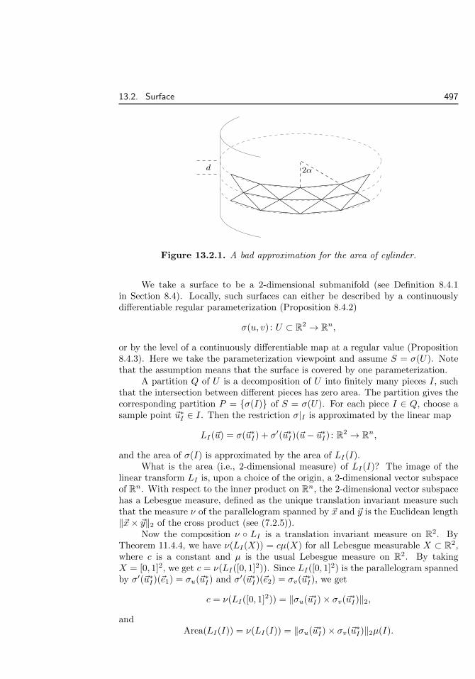
13.2. Surface 497
d 2α
Figure 13.2.1. A bad approximation for the area of cylinder.
We take a surface to be a 2-dimensional submanifold (see Definition 8.4.1in Section 8.4). Locally, such surfaces can either be described by a continuouslydifferentiable regular parameterization (Proposition 8.4.2)
σ(u, v) : U ⊂ R2 → Rn,
or by the level of a continuously differentiable map at a regular value (Proposition8.4.3). Here we take the parameterization viewpoint and assume S = σ(U). Notethat the assumption means that the surface is covered by one parameterization.
A partition Q of U is a decomposition of U into finitely many pieces I, suchthat the intersection between different pieces has zero area. The partition gives thecorresponding partition P = σ(I) of S = σ(U). For each piece I ∈ Q, choose asample point ~u∗I ∈ I. Then the restriction σ|I is approximated by the linear map
LI(~u) = σ(~u∗I) + σ′(~u∗I)(~u− ~u∗I) : R2 → Rn,
and the area of σ(I) is approximated by the area of LI(I).What is the area (i.e., 2-dimensional measure) of LI(I)? The image of the
linear transform LI is, upon a choice of the origin, a 2-dimensional vector subspaceof Rn. With respect to the inner product on Rn, the 2-dimensional vector subspacehas a Lebesgue measure, defined as the unique translation invariant measure suchthat the measure ν of the parallelogram spanned by ~x and ~y is the Euclidean length‖~x× ~y‖2 of the cross product (see (7.2.5)).
Now the composition ν LI is a translation invariant measure on R2. ByTheorem 11.4.4, we have ν(LI(X)) = cµ(X) for all Lebesgue measurable X ⊂ R2,where c is a constant and µ is the usual Lebesgue measure on R2. By takingX = [0, 1]2, we get c = ν(LI([0, 1]2)). Since LI([0, 1]2) is the parallelogram spannedby σ′(~u∗I)(~e1) = σu(~u∗I) and σ′(~u∗I)(~e2) = σv(~u
∗I), we get
c = ν(LI([0, 1]2)) = ‖σu(~u∗I)× σv(~u∗I)‖2,
andArea(LI(I)) = ν(LI(I)) = ‖σu(~u∗I)× σv(~u∗I)‖2µ(I).

498 Chapter 13. Multivariable Integration
Thus the area of the surface is approximated by∑I∈Q
Area(LI(I)) =∑I∈Q‖σu(~u∗I)× σv(~u∗I)‖2µ(I) = S(Q, ‖σu × σv‖2).
This is the Riemann sum for the integral of the function ‖σu×σv‖2 on U . Thereforethe surface area is
µ(S) =
∫U
‖σu × σv‖2dudv =
∫U
√‖σu‖22‖σv‖22 − (σu · σv)2dudv.
We also denote
dA = ‖σu × σv‖2dudv,
where A indicates the area.Intuitively, the area of a surface should be independent of the parameteriza-
tion. To verify the intuition, we consider a continuously differentiable change ofvariable (the map is invertible, and both the map and its inverse are continuouslydifferentiable)
(u, v) = (u(s, t), v(s, t)) : V → U.
We have σs = usσu + vsσv, σt = utσu + vtσv, and by (7.2.4),
σs × σt = det∂(u, v)
∂(s, t)σu × σv. (13.2.1)
Then by the change of variable formula (Theorem 12.4.5), we have∫V
‖σs×σt‖2dsdt =
∫V
∣∣∣∣det∂(u, v)
∂(s, t)
∣∣∣∣ ‖σu×σv‖2dsdt =
∫U
‖σu×σv‖2dudv. (13.2.2)
Example 13.2.2. The graph of a continuously differentiable function f(x, y) defined for(x, y) ∈ U is naturally parameterized as σ(x, y) = (x, y, f(x, y)). By
σx × σy = (1, 0, fx)× (0, 1, fy) = (−fx,−fy, 1),
the area of the surface is∫U
‖(1, 0, fx)× (0, 1, fy)‖2dxdy =
∫U
√1 + f2
x + f2ydxdy.
In case z = f(x, y) is implicitly defined by g(x, y, z) = c, we may use the implicit differen-tiation to calculate zx, zy and then substitute as fx, fy above to get∫
U
√g2x + g2
y + g2z
|gz|dxdy =
∫U
dxdy
cos θ.
Here ∇g = (gx, gy, gz) is normal to the tangent space, and θ is the angle between thetangent plane and the (x, y)-plane.

13.2. Surface 499
Example 13.2.3 (Pappus-Guldinus). Suppose C is a continuously differentiable curve in R2
parameterized by φ(t) = (x(t), y(t)), t ∈ [a, b], such that y(t) > 0. The rotation of C withrespect to the x-axis is the parameterized surface
σ(t, θ) = (x(t), y(t) cos θ, y(t) sin θ) : [a, b]× [0, 2π)→ R3.
Since the tangent vectors σt = (x′, y cos θ, y′ sin θ) and σθ = (0,−y sin θ, y cos θ) are or-thogonal, we have
‖σt × σθ‖2 = ‖σt‖2‖σθ‖2 = y√x′2 + y′2.
Therefore the area is∫[a,b]×[0,2π)
y√x′2 + y′2dtdθ = 2π
∫ b
a
y√x′2 + y′2dt = 2π
∫C
yds.
In terms of the center of weight for the curve C
(x∗C , y∗C) =
1
µ(C)
∫C
(x, y)ds,
the area is 2πy∗Cµ(C).Note that y∗C is the average of the distance from points in C to the x-axis. For a
curve C lying on the positive side of a straight line L : ax+ by = c, the area of the surfaceobtained by rotating C around L is 2πdµ(C), where
d =ax∗C + by∗C − c√
a2 + b2
is the distance from the centre of weight (x∗C , y∗C) to L, and is also the average distance
from the points on C to L.For example, the torus is obtained by rotating a circle of radius a around a straight
line of distance b away. The distance b is between the center of the circle and the line, andis also the average distance d. Therefore the torus has area 4π2ab.
Example 13.2.4. The parameterized surface in R4
σ(u, v) = (cos(u+ v), sin(u+ v), cosu, sinu), u, v ∈[0,π
2
]has area ∫
[0,π2 ]
√‖σu‖22‖σv‖22 − (σu · σv)2dudv =
∫[0,π2 ]
√2 · 1− 12dudv =
π2
4.
Exercise 13.37. Find the area of the graph of a map (f(x, y), g(x, y)) : R2 → R2, which isa surface in R4. More generally, find the area of the graph of a map F : R2 → Rn−2.
Exercise 13.38. Find the area of the surface in R4 implicitly defined as f(x, y, z, w) = aand g(x, y, z, w) = b, similar to the formula in Example 13.2.2.
Exercise 13.39. Study the effect of transforms of Rn on the area of surface.
1. For the shifting ~x→ ~a+ ~x, prove µ(~a+ S) = µ(S).
2. For the scaling ~x→ c~x, prove µ(cS) = c2µ(S).

500 Chapter 13. Multivariable Integration
3. For an orthogonal linear transform U , prove µ(U(S)) = µ(S).
The discussion above assumes that the whole surface is covered by one (con-tinuously differentiable and regular) parameterization. In general, we may not beable (or not convenient) to do so. Then we need to decompose S into finitely manysmaller pieces Si, so that the intersection among different pieces have zero area (forexample, have dimension ≤ 1). The pieces should be small enough so that each iscovered by one parameterization. Then we can use the earlier formula to computethe area of each Si, and the sum of the areas of Si is the area of S.
It remains to explain that the result of the computation is independent ofthe choice of the pieces Si and their parameterizations. Suppose S′j is anotherdecomposition, and each S′j has a regular parameterization. Then S is furtherdecomposed into the intersections S′′ij = Si ∩ S′j . Each S′′ij can be parameterizedeither as Si or as S′j . By Si = ∪jS′′ij , where the intersections of different pieces havezero area, the area of S computed from Si is∑
i
µ(Si) =∑i
∑j
µ(S′′ij ,parameterized as Si).
Similarly, the area of S computed from S′j is∑j
µ(S′j) =∑j
∑i
µ(S′′ij ,parameterized as S′j).
Since we have argued in (13.2.2) that the two parameterizations of S′′ij give the samearea µ(S′′ij), the two sums are equal.
Integration of Function Along Surface
The integration of a function f(~x) along a surface S covered with one regular pa-rameterization σ(u, v) : U ⊂ R2 → Rn is∫
S
fdA =
∫U
f(σ(u, v))‖σu(u, v)× σv(u, v)‖2dudv.
In general, we may need to divide the surface into smaller parameterized pieces,such that the intersections of different pieces have zero area. Then we add theintegrals on the pieces together.
By an argument similar to (13.2.2), the integral is independent of the choiceof the parameterization∫
S
fdA =
∫V
f(σ(s, t))‖σs × σt‖2dsdt
=
∫V
f(σ(s, t))
∣∣∣∣det∂(u, v)
∂(s, t)
∣∣∣∣ ‖σu × σv‖2dsdt (13.2.3)
=
∫U
f(σ(u, v))‖σu × σv‖2dudv.

13.2. Surface 501
Here the first equality is the definition of
∫S
fdA in terms of the parameter (s, t),
the second is the change of variable formula, the third is by (13.2.1), and the last
expression is the definition of
∫S
fdA in terms of the parameter (u, v).
We may further show that the integral is also independent of the decompositionof the surface into parameterized pieces. Moreover, the integral has propertiessimilar to the integral of functions along rectifiable curves.
Example 13.2.5. For a fixed vector ~a ∈ R3, consider the integral
∫S2
f(~a ·~x)dA on the unit
sphere. There is a rotation that moves ~a to (r, 0, 0), r = ‖~a‖2. Since the rotation preservesthe surface area, we have∫
S2
f(~a · ~x)dA =
∫S2
f((r, 0, 0) · (x, y, z))dA =
∫S2
f(rx)dA.
Parametrize S2 by σ(x, θ) = (x,√
1− x2 cos θ,√
1− x2 sin θ). Then ‖σx × σθ‖2 = 1 and∫S2
f(rx)dA =
∫−1≤x≤10≤θ≤2π
f(rx)dxdθ = 2π
∫ 1
−1
f(rx)dx =2π
‖~a‖2
∫ ‖~a‖2−‖~a‖2
f(x)dx.
Exercise 13.40. Study the effect of transforms of Rn on the integral along surface.
1. For the shifting ~x→ ~a+ ~x, prove
∫~a+S
f(~x)dA =
∫S
f(~a+ ~x)dA.
2. For the scaling ~x→ c~x, prove
∫cS
f(~x)dA = c2∫S
f(c~x)dA.
3. For an orthogonal linear transform U , prove
∫U(S)
f(~x)dA =
∫S
f(U(~x))dA.
Exercise 13.41. Compute the attracting force
∫S2
~x− ~a‖~x− ~a‖32
dA of the unit sphere on a point
~a.
Exercise 13.42. Prove that the definition of
∫S
fdA is independent of the decomposition of
the surface into parameterized pieces.
Integration of 2-Form Along Surface
Suppose σ(u, v) : U ⊂ R2 → R3 is a continuously differentiable regular parameteri-zation of a surface S ⊂ R3. Then the parameterization gives a normal vector
~n =σu × σv‖σu × σv‖2
.
Geometrically, the normal vector is determined by the following properties:
• Direction: ~n is orthogonal to the tangent plane of S.

502 Chapter 13. Multivariable Integration
• Length: ~n has Euclidean norm 1.
• Orientation: ~n, σu, σv follows the “right hand rule”, which means thatdet(~n σu σv) > 0.
The first property means ~n · σu = 0 and ~n · σv = 0. The first two properties areindependent of the choice of the parameterization and determine the normal vectorup to the choice among ~n and −~n. The orientation picks one from the two choices.
In general, we may need to divide the surface into parameterized pieces Si.Then we need the normal vectors of the piece to be compatible in the sense that thenormal vector changes continuously when we move from one piece to another. Thenthe whole surface has a continuous choice of the normal vectors. Such a choice iscalled an orientation, and the surface is called orientable.
It is possible for a surface to be nonorientable in the sense that there is nocontinuous choice of the normal vectors. This is equivalent to the nonexistenceof a collection of compatibly oriented parameterizations. A typical example is theMobius band. In fact, a surface is not orientable if and only if it contains a Mobiusband.
Figure 13.2.2. The Mobius band is not orientable.
Example 13.2.6. The graph of a continuously differentiable function f(x, y) is naturallyparameterized as σ(x, y) = (x, y, f(x, y)). By
σx × σy = (1, 0, fx)× (0, 1, fy) = (−fx,−fy, 1),
the normal vector induced by the parameterization is
~n =σx × σy‖σx × σy‖
=(−fx,−fy, 1)√f2x + f2
y + 1.
Alternatively, we may try to find ~n by using the three characteristic properties. Firstwe solve for ~v = (a, b, c)
~v · σx = a+ cfx = 0, ~v · σy = b+ cfy = 0.
Choosing c = 1, we get ~v = (−fx,−fy, 1), which is parallel to ~n. Then by
det(~v σx σy) = det
−fx 1 0−fy 0 1
1 fx fy
= f2x + f2
y + 1 > 0,
we know ~n and ~v point to the same direction. Since ~n has the unit length, we get
~n =~v
‖~v‖ =(−fx,−fy, 1)√f2x + f2
y + 1.

13.2. Surface 503
Example 13.2.7. The sphere S2R = (x, y, z) : x2+y2+z2 = R2 of radius R can be covered
by the paramerizations
σ1(x, y) = (x, y,√R2 − x2 − y2), x2 + y2 < R2,
σ2(y, x) = (x, y,−√R2 − x2 − y2), x2 + y2 < R2,
σ3(z, x) = (x,√R2 − x2 − z2, z), x2 + z2 < R2,
σ4(x, z) = (x,−√R2 − x2 − z2, z), x2 + z2 < R2,
σ5(y, z) = (√R2 − y2 − z2, y, z), y2 + z2 < R2,
σ6(z, y) = (−√R2 − y2 − z2, y, z), y2 + z2 < R2.
By
(σ1)x × (σ1)y =(
1, 0,−xz
)×(
0, 1,−yz
)=(xz,y
z, 1),
the normal vector from the first parameterization is
(σ1)x × (σ1)y‖(σ1)x × (σ1)y‖2
=(x, y, z)
‖(x, y, z)‖2=~x
R.
Similar computations also show that~x
Ris the normal vector from the other parameteri-
zations. Therefore the choice ~n =~x
Rgives an orientation of the sphere.
Note that the order of the variables in σ2 are deliberately arranged to have y as thefirst and x as the second. Thus the normal vector should be computed from (σ2)y × (σ2)xinstead of the other way around.
Like a vector field along a curve, a vector field along a surface is a mapF : S → Rn. If S is orientable, with orientation ~n, then the flux of the vector fieldalong the surface is∫
S
F · ~ndA =
∫U
F (σ(u, v)) · (σu(u, v)× σv(u, v))dudv.
The left side shows that the integral is independent of the choice of the parameter-ization, as long as the parameterization is compatible with the orientation, in thesense that σu×σv is a positive multiple of ~n. In fact, changing the orientation from~n to −~n changes the integral by a negative sign. This is similar to the effect on∫C
F · d~x when we reverse the orientation of C.
Example 13.2.8. The outgoing flux of the flow F = (x2, y2, z2) through the sphere ‖~x −~x0‖22 = (x− x0)2 + (y − y0)2 + (z − z0)2 = R2 is∫
‖~x−~x0‖2=R
(x2, y2, z2) · (x− x0, y − y0, z − z0)
RdA.
By the shifting ~x→ ~x0 + ~x, the integral is equal to
1
R
∫‖~x‖2=R
((x+ x0)2x+ (y + y0)2y + (z + z0)2z)dA.

504 Chapter 13. Multivariable Integration
By suitable rotations that exchange the axis, we have∫‖~x‖2=R
xndA =
∫‖~x‖2=R
yndA =
∫‖~x‖2=R
zndA.
By the transform (x, y, z) → (−x, y, z), we also know that the first integral vanishes forodd integers n. Thus the integral above becomes
1
R
∫‖~x‖2=R
(2x0x2 + 2y0y
2 + 2z0z2)dA =
2
R(x0 + y0 + z0)
∫‖~x‖2=R
x2dA.
Then we further use the equalities above to get∫‖~x‖2=R
x2dA =1
3
∫‖~x‖2=R
(x2 + y2 + z2)dA =1
3
∫‖~x‖2=R
R2dA =1
3R2 · 4πR2 =
4
3πR4.
We conclude that the flux is8
3π(x0 + y0 + z0)R3.
Exercise 13.43. Study the effect of transforms of Rn on the flux, similar to Exercise 13.40.
Exercise 13.44. By an argument similar to (13.2.3), prove that
∫S
F · ~ndA is not changed
by compatible change of variable.
Now we give a formal interpretation of the flux. For the parameterizationσ(u, v) = (x(u, v), y(u, v), z(u, v)), by formally taking the cross product of differen-tial 1-forms, we have
dx× dy = (xudu+ xvdv)× (yudu+ yvdv)
= (xuyv − xvyu)du× dv = det∂(x, y)
∂(u, v)du× dv,
and the similar formulae for dy × dz and dz × dx. Then for F = (f, g, h), we have
[F · (σu × σv)]du× dv= [f(yuzv − yvzu) + g(zuxv − zvxu) + h(xuyv − xvyu)]du× dv= fdy × dz + gdz × dx+ hdx× dy.
This suggests that the flux
∫S
F ·~ndA should really be denoted
∫S
fdy×dz+gdz×dx+ hdx× dy.
Since the cross product is a special case of the exterior product, we introducethe differential 2-form on R3
ω = fdy ∧ dz + gdz ∧ dx+ hdx ∧ dy.
Then the flux may be interpreted as the integral of the differential 2-form on anoriented surface∫
S
fdy ∧ dz + gdz ∧ dx+ hdx ∧ dy
=
∫U
(f det
∂(y, z)
∂(u, v)+ g det
∂(z, x)
∂(u, v)+ hdet
∂(x, y)
∂(u, v)
)dudv. (13.2.4)

13.2. Surface 505
The formula is only for one piece of the regular parameterization σ(u, v), such thatσu × σv is a positive multiple of ~n. In general, we need to divide the surface intosuch pieces and add the integrals on the pieces together.
The use of exterior product allows us to extend the integral of 2-forms to moregeneral orientable surfaces. A differential 2-form on Rn is
ω =∑
1≤i<j≤n
fij(~x)dxi ∧ dxj ,
and its integral on a surface S ⊂ Rn regularly parameterized by continuously dif-ferentiable map σ(u, v) : U ⊂ R2 → Rn is∫
S
ω =∑
1≤i<j≤n
∫U
fij(σ(u, v)) det∂(xi, xj)
∂(u, v)dudv. (13.2.5)
Under a change of variable between (u, v) ∈ U and (s, t) ∈ V , we have (see Theorem12.4.5) ∫
U
f(σ(u, v)) det∂(xi, xj)
∂(u, v)dudv
=
∫V
f(σ(s, t)) det∂(xi, xj)
∂(u, v)
∣∣∣∣det∂(u, v)
∂(s, t)
∣∣∣∣ dsdt.Since
∂(xi, xj)
∂(s, t)=∂(xi, xj)
∂(u, v)
∂(u, v)
∂(s, t), the right side fits into the definition (13.2.6) in
terms of the new variable (s, t) if and only if det∂(u, v)
∂(s, t)> 0. This is the condition
for (13.2.6) to be well defined.
In case n = 3, by (13.2.1), the condition det∂(u, v)
∂(s, t)> 0 means exactly that
both parameterizations give the same normal vector. Although we no longer havethe normal vector for general n, we may still talk about compatible parameteriza-
tions in the sense that det∂(u, v)
∂(s, t)> 0. Therefore we say a surface S ⊂ Rn is oriented
if it is covered by finitely many parameterized pieces σi : Ui ⊂ R2 → Si ⊂ Rn, whereSi are open subsets of S and S = ∪Si, such that the transition maps (see Figure14.1.1)
ϕji = σ−1j σi : Uij = σ−1
i (Si ∩ Sj)→ Uji = σ−1j (Si ∩ Sj)
on the overlapping of pieces satisfy
detϕ′ji > 0 for any i, j.
Such a collection σi gives an orientation of the surface. Any other parameteriza-tion σ∗ : U ⊂ R2 → S∗ ⊂ S is compatible with the orientation if det(σ−1
i σ∗)′ > 0on σ−1(S∗ ∩ Si).

506 Chapter 13. Multivariable Integration
S
Uij ϕji
Uji
σi
Si
σj
Sj
Figure 13.2.3. Transition map between overlapping parameterizations.
We would like to define the integral of a 2-form ω on an oriented surface as
∫S
ω =∑k
∫Sk
ω =∑k
∑1≤i<j≤n
∫Uk
fij(σk(u, v)) det∂(xi, xj)
∂(u, v)dudv.
However, we need to take into account of the overlapping between pieces, where theintegral is computed more than once. A practical way to get around this is to findsubsets Bk ⊂ Uk, such that S = ∪kσk(Bk) and σk(Bk) ∩ σl(Bl) has zero area forany k 6= l. Then define
∫S
ω =∑k
∑1≤i<j≤n
∫Bk
fij(σk(u, v)) det∂(xi, xj)
∂(u, v)dudv. (13.2.6)
A more theoretical way is to use the partition of unity. See the theory of calculuson manifolds.
Example 13.2.9. We compute the outgoing flux of F = (x2, y2, z2) in Example 13.2.8
through the ellipse S given by(x− x0)2
a2+
(y − y0)2
b2+
(z − z0)2
c2= 1. By the shifting
~x→ ~x0 + ~x, the flux is the integral
∫S+~x0
(x+ x0)2dy ∧ dz + (y + y0)2dz ∧ dx+ (z + z0)2dx ∧ dy.
The integral of (z + z0)2dx ∧ dy may be computed by using parameterizations similar to

13.2. Surface 507
σ1 and σ2 in Example 13.2.7
∫S−~x0
(z + z0)2dx ∧ dy =
∫x2
a2+ y2
b2≤1
(c
√1− x2
a2− y2
b2+ z0
)2
det∂(x, y)
∂(x, y)dxdy
+
∫x2
a2+ y2
b2≤1
(−c√
1− x2
a2− y2
b2+ z0
)2
det∂(x, y)
∂(y, x)dxdy
= 4z0c
∫x2
a2+ y2
b2≤1
√1− x2
a2− y2
b2dxdy
= 4abcz0
∫u2+v2≤1
√1− u2 − v2dudv =
8
3πabcz0.
The total flux is8
3πabc(x0 + y0 + z0).
Example 13.2.10. Let S be the surface parameterised by σ(u, v) = (u+v, u2 +v2, . . . , un+vn) for 0 ≤ u ≤ a, 0 ≤ v ≤ b. The parameterization gives an orientation of the surface.With respect to this orientation, the integral∫
S
dx1 ∧ dx2 + dx2 ∧ dx3 + · · ·+ dxn−1 ∧ dxn
=
∫S
(det
∂(x1, x2)
∂(u, v)+ det
∂(x2, x3)
∂(u, v)+ · · ·+ det
∂(xn−1, xn)
∂(u, v)
)dudv
=
∫ a
0
∫ b
0
[det
(1 1
2u 2v
)+ det
(2u 2v3u2 3v2
)+ · · ·+ det
((n− 1)un−2 (n− 1)vn−2
nun−1 nvn−1
)]dudv
=
∫ a
0
∫ b
0
[1 · 2(v − u) + 2 · 3(uv2 − u2v) + · · ·+ (n− 1)n(un−2vn−1 − un−1vn−2)]dudv
= (ab2 − a2b) + (a2b3 − a3b2) + · · ·+ (an−1bn − anbn−1)
= (b− a)(ab+ a2b2 + · · ·+ an−1bn−1) =(b− a)(1− anbn)
1− ab .
Exercise 13.45. Compute the integral of 2-form.
1.
∫S
xy2dy ∧ dz + yz2dz ∧ dx + zx2dx ∧ dy, S is the ellipse(x− x0)2
a2+
(y − y0)2
b2+
(z − z0)2
c2= 1 with orientation given by the inward normal vector.
2.
∫S
xyzdx ∧ dy, S is the part of the ellipsex2
a2+y2
b2+z2
c2= 1, x ≥ 0, y ≥ 0, with
orientation given by outward normal vector.
3.
∫S
xydy∧dz and
∫S
x2ydy∧dz, S is the boundary of the solid enclosed by z = x2+y2
and z = 1, with orientation given by outward normal vector.

508 Chapter 13. Multivariable Integration
Exercise 13.46. Prove that the area of a surface S ⊂ R3 given by an equation g(x, y, z) = c
is
∫S
gxdy ∧ dz + gydz ∧ dx+ gzdx ∧ dy√g2x + g2
y + g2z
.
13.3 SubmanifoldThe integration along curves and surfaces can be extended to higher dimensionalsubmanifolds.
Volume and Integration of Function
Suppose M is a k-dimensional submanifold of Rn. If M is regularly parameterizedby continuously differentiable σ(~u) : U ⊂ Rk → Rn, then the volume of M is
µ(M) =
∫U
‖σu1∧ · · · ∧ σuk‖2du1 · · · duk.
The definition is independent of the choice of parameterization. We also denote thevolume unit
dV = ‖σu1 ∧ · · · ∧ σuk‖2du1 · · · duk
=√
det(σui · σuj )1≤i,j≤kdu1 · · · duk
=
√√√√ ∑1≤i1<···<in≤N
(det
∂(xi1 , . . . , xin)
∂(u1, . . . , un)
)2
du1 · · · dun. (13.3.1)
The integral of a function along the submanifold is∫M
fdV =
∫U
f(σ(u1, . . . , uk))‖σu1 ∧ · · · ∧ σuk‖2du1 · · · duk
The integral is also independent of the choice of parameterization.
Example 13.3.1. Let F (~θ) : U ⊂ Rn−1 → Rn be a parameterization of the unit sphereSn−1. Since F ·F = ‖F‖22 = 1, by taking partial derivatives, we get Fθi ·F = 0. ThereforeF is a unit length vector orthogonal to Fθi . This implies that
‖Fθ1 ∧ Fθ2 ∧ · · · ∧ Fθn−1‖2 = ‖F ∧ Fθ1 ∧ Fθ2 ∧ · · · ∧ Fθn−1‖2 = | det(F F ′)|,
so that the volume of the sphere Sn−1 is
βn−1 =
∫U
‖Fθ1 ∧ Fθ2 ∧ · · · ∧ Fθn−1‖2dµ~θ =
∫U
| det(F F ′)|dµ~θ.
The parameterization F (~θ) induces a parameterization of Sn
G(~θ, φ) = (F (~θ) cosφ, sinφ) : U ×[−π
2,π
2
]→ Rn+1.

13.3. Submanifold 509
We have
‖Gθ1 ∧Gθ2 ∧ · · · ∧Gθn−1 ∧Gφ‖2= ‖(Fθ1 cosφ, 0) ∧ (Fθ2 cosφ, 0) ∧ · · · ∧ (Fθn−1 cosφ, 0) ∧ (−F sinφ, cosφ)‖2= ‖(Fθ1 cosφ, 0) ∧ (Fθ2 cosφ, 0) ∧ · · · ∧ (Fθn−1 cosφ, 0)‖2‖(−F sinφ, cosφ)‖2= ‖Fθ1 ∧ Fθ2 ∧ · · · ∧ Fθn−1‖2 cosn−1 φ,
where the second equality is due to (−F sinφ, cosφ) ⊥ (Fθi cosφ, 0), and the last equalityis due to
‖(−F sinφ, cosφ)‖2 =√‖F‖22 sin2 φ+ cos2 φ =
√sin2 φ+ cos2 φ = 1.
Therefore
βn =
∫~θ∈A
−π2≤φ≤π
2
‖Fθ1 ∧ Fθ2 ∧ · · · ∧ Fθn−1‖2 cosn−1 φdµ~θdφ = βn−1
∫ π2
−π2
cosn−1 φdφ.
Using integration by parts, we get
∫ π2
−π2
cosn φdφ =n− 1
n
∫ π2
−π2
cosn−2 φdφ = · · · =
(n− 1)(n− 3) · · · 1n(n− 2) · · · 2 π, if n is even,
(n− 1)(n− 3) · · · 2n(n− 2) · · · 3 2, if n is odd.
Therefore βn =2π
n− 1βn−2. Combined with β1 = 2π, β2 = 4π, we get
βn−1 =
2πk
(k − 1)!, if n = 2k,
2k+1πk
(2k − 1)(2k − 3) · · · 1 , if n = 2k + 1.
We also note that
H(r, ~θ) = rF (~θ) : (0,∞)×A→ Rn
is a spherical change of variable. We have H ′ = (F rF ′), detH ′ = rn−1 det(F F ′), so that∫a≤‖~x‖2≤b
f(‖~x‖2)dµ =
∫~θ∈Aa≤r≤b
f(r)rn−1|det(F F ′)|drdµ~θ = βn−1
∫ b
a
f(r)rn−1dr.
In particular, by taking f = 1, a = 0, b = 1, we get the volume of the unit ball Bn
αn = βn−1
∫ 1
0
rn−1dr =βn−1
n=
πk
k!, if n = 2k,
2k+1πk
(2k + 1)(2k − 1)(2k − 3) · · · 1 , if n = 2k + 1.
Example 13.3.2. Consider a k-dimensional submanifold M parameterized by
σ(~u) = (ξ(~u), r(~u)) : U ⊂ Rk → Rn × R.

510 Chapter 13. Multivariable Integration
Assume r(~u) ≥ 0, so that the submanifold is inside the upper half Euclidean space. Thel-dimensional rotation of M around the axis Rn × 0 is a (k + l)-dimensional submanifold
ρl(M) = (~x, ~y) ∈ Rn × Rl+1 : (~x, ‖~y‖2) ∈ S.
Let F (~θ) : V ⊂ Rl → Rl+1 be a parameterization of the unit sphere Sl. Then the rotationsubmanifold ρl(M) is parameterized by
ρ(~u, ~θ) = (ξ(~u), r(~u)F (~θ)) : U × V → Rn × Rl+1.
By ρui = (ξui , ruiF ), ρθj = (~0, rFθj ), and ρui · ρθj = ruiF · rFθj = 0, we get
‖ρu1 ∧ρu2 ∧· · ·∧ρuk ∧ρθ1 ∧ρθ2 ∧· · ·∧ρθl‖2 = ‖ρu1 ∧ρu2 ∧· · ·∧ρuk‖2‖ρθ1 ∧ρθ2 ∧· · ·∧ρθl‖2,
and
‖ρθ1 ∧ ρθ2 ∧ · · · ∧ ρθl‖2 = rl‖Fθ1 ∧ Fθ2 ∧ · · · ∧ Fθl‖2.Moreover, there is an orthogonal transform UF on Rl+1 such that UF (F ) = (1, 0, . . . , 0).Then (id, UF ) is an orthogonal transform on Rn × Rl+1 such that
(id, UF )ρui = (ξui , ruiUF (F )) = (ξui , rui , 0, . . . , 0) = (σui , 0, . . . , 0).
Applying the orthogonal transform to ‖ρu1 ∧ ρu2 ∧ · · · ∧ ρuk‖2, we get
‖ρu1 ∧ ρu2 ∧ · · · ∧ ρuk‖2 = ‖σu1 ∧ σu2 ∧ · · · ∧ σuk‖2
Thus the volume of the rotation hypersurface is
µ(ρl(S)) =
∫U×V
‖σu1 ∧ σu2 ∧ · · · ∧ σuk‖2rl‖Fθ1 ∧ Fθ2 ∧ · · · ∧ Fθl‖2dµ~udµ~θ
= βl
∫U
‖σu1 ∧ σu2 ∧ · · · ∧ σuk‖2rldµ~u = βl
∫S
rldV.
Exercise 13.47. Use the rotation in Example 13.3.2 to prove that
βk+l+1 = βkβl
∫ π2
0
cosk θ sinl θdθ.
Exercise 13.48. Extend the result of Example 13.3.2 to the rotation around a hyperplane~a · ~x = b (the surface is on the positive side of the hyperplane).
Integration of Differential Form
A differential k-form on Rn is
ω =∑
i1<···<ik
fi1···ik(~x)dxi1 ∧ · · · ∧ dxik . (13.3.2)
Its integral on a regularly parameterized k-dimensional submanifold M is∫M
ω =
∫U
fi1···ik(σ(u1, . . . , uk)) det∂(xi1 , . . . , xik)
∂(u1, . . . , uk)du1 · · · duk.

13.3. Submanifold 511
Similar to the integral of differential 2-forms on surfaces, the integral is independentof the parameterizations as long as they are compatibly oriented. The compatibilitymeans that the determinant of the Jacobian for the change of variables (so calledtransition map) is positive. In general, the submanifold may be divided into severalcompatibly oriented pieces, and the integral of the differential form is the sumof the integrals on the pieces (strictly speaking, on smaller pieces such that theoverlappings have zero volume).
Now we consider the special case of the integral of an (n − 1)-form on anoriented (n − 1)-dimensional submanifold M ⊂ Rn. What is special here is theexistence of the normal vector. Similar to parameterized surfaces in R3, the normalvector is determined by the following properties:
• Direction: ~n · σui = 0 for i = 1, . . . , n− 1.
• Length: ‖~n‖2 = 1.
• Orientation: det(~n σu1· · · σun−1
) > 0.
By the first property and (7.4.2), we have
(σu1∧ · · · ∧ σun−1
)? = c~n,
wherec = det(σu1 · · · σun−1 ~n) = (−1)n−1 det(~n σu1 · · · σun−1).
Then by the second and third properties, we get
~n = (−1)n−1 (σu1∧ · · · ∧ σun−1
)?
‖σu1∧ · · · ∧ σun−1
‖2.
Let (xi means the term xi is missing from the list)
~a = (σu1 ∧ · · · ∧ σun−1)? =∑
det∂(x1, . . . , xi, . . . , xn)
∂(u1, . . . , un−1)~e ?∧([n]−i)
=∑
(−1)n−i det∂(x1, . . . , xi, . . . , xn)
∂(u1, . . . , un−1)~ei.
Then the flux of a vector field F = (f1, . . . , fn) along the oriented M is∫M
F · ~ndV = (−1)n−1
∫A
F · ~adu1 · · · duk
=
∫U
∑(−1)i−1fi det
∂(x1, . . . , xi, . . . , xn)
∂(u1, . . . , un−1)du1 · · · duk
=
∫M
∑(−1)i−1fidx1 ∧ · · · ∧ dxi ∧ · · · ∧ dxn. (13.3.3)
If n = 3, then M is a surface in R3, and (−1)3−1(σu1∧σu2
)∗ is the usual crossproduct σu1
× σu2. Therefore (13.3.3) is the usual flux along an oriented surface in
R3.

512 Chapter 13. Multivariable Integration
If n = 2, then M is a curve φ(t) in R2. The property det(~n φ′(t)) > 0 impliesthat the normal vector ~n is the clockwise rotation of the unit length tangent vector
~t =φ′(t)
‖φ′(t)‖by 90 degrees. The rotation is R(x, y) = (y,−x), so that
∫C
(f, g) · ~nds =
∫C
(f, g) ·R(~t)ds =
∫C
R−1(f, g) · ~tds
=
∫C
(−g, f) · d~x =
∫C
fdy − gdx.
~t
~n
Figure 13.3.1. Normal vector of oriented curve
Example 13.3.3. Consider the graph σ(~u) = (~u, f(~u)), ~u = (x1, . . . , xn−1), of a continu-ously differentiable function f on Rn−1. By
(σx1 ∧ · · · ∧ σxn−1)?
= ((~e1 + fx1~en) ∧ · · · ∧ (~en−1 + fxn−1~en))?
= (~e1 ∧ · · · ∧ ~en−1)? +∑
(−1)n−1−ifxi(~e1 ∧ · · · ∧ ~ei ∧ · · · ∧ ~en)?
= ~en −∑
fxi~ei = (−fx1 , . . . ,−fxn−1 , 1),
the normal vector
~n = (−1)n−1 (−fx1 , . . . ,−fxn−1 , 1)√f2x1 + · · ·+ f2
xn−1+ 1
points in the direction of xn for odd n and opposite to the direction of xn for even n.Another way of finding ~n is by using the three characteristic properties, similar to
Example 13.2.6. First, for ~v = (a1, . . . , an), we solve
~v · σxi = (v1, . . . , vn) · (0, . . . , 1(i), . . . , 0, fxi) = vi + vnfxi = 0.
By taking vn = 1, we get one solution ~v = (−fx1 , . . . ,−fxn−1 , 1). Moreover,
det(~v σx1 · · · σxn−1) = det
−fx1 1 0 · · · 0−fx2 0 1 · · · 0
......
......
−fxn−1 0 0 · · · 11 fx1 fx2 · · · fxn−1
= (−1)n−1(f2
x1 + · · ·+ f2xn−1
+ 1).

13.3. Submanifold 513
Therefore we get
~n = (−1)n−1 ~v
‖~v‖ = (−1)n−1 (−fx1 , . . . ,−fxn−1 , 1)√f2x1 + · · ·+ f2
xn−1+ 1
.
Exercise 13.49. Suppose U is an orthogonal transform of Rn. Prove that if ~n is the normalvector of a regular parameterzation σ(~u), then (detU)U(~n) is the normal vector of theregular parameterzation U(σ(~u)). Moreover, use this to show that the normal vector ofthe graph
σi(~u) = (x1, . . . , xi−1, f(~u), xi+1, . . . , xn), ~u = (x1, . . . , xi, . . . , xn),
of a continuously differentiable function f is
(−1)i−1 (−fx1 , . . . ,−fxi−1 , 1,−fxi+1 , . . . ,−fxn)√f2x1 + · · ·+ f2
xi + · · ·+ f2xn + 1
.
Exercise 13.50. Justify the normal vector in Exercise 13.49 by verifying the geometricalcharacterization.
Exercise 13.51. The unit sphere Sn in Rn+1 has the normal vector ~n = ~x at ~x ∈ Sn. Foreach 0 ≤ i ≤ n, find suitable rearrangements (xk0 , . . . , xki , . . . , xkn) and (xl0 , . . . , xli , . . . , xln)of (x0, . . . , xi, . . . , xn), such that the parameterizations
σ+i (x0, . . . , xi, . . . , xn) = (xk0 , . . . , xki−1 ,
√1− x2
0 − · · · − x2i − · · · − x2
n, xki+1 , . . . , xkn),
σ−i (x0, . . . , xi, . . . , xn) = (xl0 , . . . , xli−1 ,−√
1− x20 − · · · − x2
i − · · · − x2n, xli+1 , . . . , xln).
cover Sn and induce the given normal vector. In particular, the parameterizations arecompatibly oriented.
Exercise 13.52. Use (13.3.3) to show that the length of a curve C in R2 given by an
equation g(x, y) = c is
∫C
−gydx+ gxdy√g2x + g2
y
, similar to the formula in Exercise 13.46. Ex-
tend the formula to the volume of an (n − 1)-dimensional hypersurface in Rn given byg(x1, x2, . . . , xn) = c.
Exercise 13.53. Compute the integral.
1.
∫Sn−1R
(~x− ~a) · ~ndV , the normal vector ~n points outward of the sphere.
2.
∫Sn−1R
(a1x1 + a2x2 + · · ·+ anxn)dx2 ∧ dx3 ∧ · · · ∧ dxn, the orientation of the sphere
is given by the outward normal vector.
3.
∫S
dx1 ∧ dx2 ∧ dx3 + dx2 ∧ dx3 ∧ dx4 + · · ·+ dxn−2 ∧ dxn−1 ∧ dxn, S is the surface
σ(u, v, w) = ρ(u) + ρ(v) + ρ(w), ρ(u) = (u, u2, . . . , un), 0 ≤ u, v, w ≤ a.

514 Chapter 13. Multivariable Integration
13.4 Green’s TheoremThe Fundamental Theorem of Calculus relates the integration of a function on aninterval to the values of the antiderivative at the end points of the integral. TheGreen’s Theorem extends the fundamental theorem to the plane.
2-Dimensional Fundamental Theorem of Calculus in R2
A curve φ : [a, b] → Rn is simple if it has no self intersection. It is closed ifφ(a) = φ(b). The concept of simple closed curve is independent of the choice ofparameterization.
A simple closed curve in R2 divides the plane into two connected pieces, onebounded and the other unbounded. Therefore we have two sides of a simple closedcurve in R2. Suppose U ⊂ R2 is a bounded subset with finitely many rectifiablesimple closed curves C1, C2, . . . , Ck as the boundary. Then Ci has a compatibleorientation such that U is “on the left” of Ci. This means that Ci has counterclock-wise orientation if U is in the bounded side of Ci, and has clockwise orientation ifU is in the unbounded side. Moreover, in case Ci is regular and differentiable, wehave the outward normal vector ~n along Ci pointing away from U . By rotating theoutward normal vector by 90 degrees in the counterclockwise direction, we get thecompatible direction ~t of Ci.
C3
~n
~t
C1
~n
~t
C2
U
Figure 13.4.1. Compatible orientation of boundary.
Theorem 13.4.1 (Green’s Theorem). Suppose U ⊂ R2 is a region with compati-bly oriented rectifiable boundary curve C. Then for any continuously differentiablefunctions f and g, we have∫
C
fdx+ gdy =
∫U
(−fy + gx)dxdy.

13.4. Green’s Theorem 515
The curve C in the theorem is understood to be the union of simple closedcurves C1, C2, . . . , Ck, each oriented in the compatible way. The integral along Cis ∫
C
=
∫C1
+
∫C2
+ · · ·+∫Ck
.
Proof. We only prove
∫C
fdx = −∫U
fydxdy. By exchanging x and y (which re-
verses the orientation), this also gives
∫C
gdy =
∫U
gxdxdy. Adding the two equal-
ities gives the whole formula.
a b
Cb
y = k(x)
Cty = h(x)
Cl
CrU
Figure 13.4.2. Green’s Theorem for a special case.
We first consider the special case that
U = (x, y) : x ∈ [a, b], h(x) ≥ y ≥ k(x)
is a region between the graphs of functions h(x) and k(x) with bounded variations.We have∫
U
fydxdy =
∫ b
a
(∫ h(x)
k(x)
fy(x, y)dy
)dx (Fubini Theorem)
=
∫ b
a
(f(x, h(x))− f(x, k(x)))dx. (Fundamental Theorem)
On the other hand, the boundary C consists of four segments with the followingorientation compatible parameterizations.
Cb : φ(t) = (t, k(t)), t ∈ [a, b]
Cr : φ(t) = (b, t), t ∈ [k(b), h(b)]
Ct : φ(t) = (−t, h(−t)), t ∈ [−b,−a]
Cl : φ(t) = (a,−t), t ∈ [−h(a),−k(a)]

516 Chapter 13. Multivariable Integration
Then ∫C
fdx =
(∫Cb
+
∫Cr
+
∫Ct
+
∫Cl
)fdx
=
∫ b
a
f(t, k(t))dt+
∫ h(b)
k(b)
f(b, t)db
+
∫ −a−b
f(−t, h(−t))d(−t) +
∫ −k(a)
−h(a)
f(a,−t)da
=
∫ b
a
f(x, k(x))dx+ 0 +
∫ a
b
f(x, h(x))dx+ 0.
Therefore we have
∫U
fydxdy = −∫C
fdx.
In general, the region U can often be divided by vertical lines into severalspecial regions Uj studied above. Let Cj be the compatibly oriented boundary of
Uj . Then the sum of
∫Cj
fdx is
∫C
fdx, because the integrations along the vertical
lines are all zero. Moreover, the sum of
∫Uj
fydxdy is
∫U
fydxdy. This proves the
equality
∫C
fdx = −∫U
fydxdy for the more general regions.
U1
U2
U3
U4
U5
U6
U8
U9
U7
Figure 13.4.3. Divide into special cases: Orientations for U1, U6 given.
Now consider the most general case that the boundary curves are assumed tobe only rectifiable. To simplify the presentation, we will assume that U has onlyone boundary curve C. Let P be a partition of C. Let L be the union of straightline segements Li connecting the partition points ~xi−1 and ~xi. Let U ′ be the regionenclosed by the curve L. Then U ′ can be divided by vertical lines into special

13.4. Green’s Theorem 517
regions. As explained above, we have∫L
fdx = −∫U ′fydxdy.
We will show that, as ‖P‖ = maxµ(Ci)→ 0, the left side converges to
∫C
fdx, and
the right side converges to −∫U
fydxdy. Then the general case is proved.
For any ε > 0, by the uniform continuity of f on compact C ∪ L, there isδ > 0, such that ~x, ~y ∈ C ∪ L and ‖~x− ~y‖ < δ imply |f(~x)− f(~y)| < ε. If ‖P‖ < δ,then for ~x ∈ Ci ∪ Li, we have |f(~x)− f(~xi)| < ε. This implies∣∣∣∣(∫
Ci
−∫Li
)f(~x)dx
∣∣∣∣ =
∣∣∣∣(∫Ci
−∫Li
)(f(~x)− f(~xi))dx
∣∣∣∣ ≤ εµ(Ci).
Therefore∣∣∣∣∫C
fdx−∫L
fdx
∣∣∣∣ ≤∑∣∣∣∣(∫Ci
−∫Li
)fdx
∣∣∣∣ ≤∑ εµ(Ci) = εµ(C).
This proves lim‖P‖→0
∫L
fdx =
∫C
fdx.
On the other hand, let M be the upper bound of the continuous function
‖∇f‖2 =√f2x + f2
y on the compact region enclosed by C and L. Let Bj be the
region bounded by Cj and Lj . Then Bj is contained in the ball of center ~xi andradius µ(Ci). Therefore the area µ(Bj) ≤ πµ(Ci)
2 ≤ πδµ(Ci), and we have∣∣∣∣∫U
fdxdy −∫U ′fdxdy
∣∣∣∣ ≤∑∫Bj
|f |dxdy
≤∑
Mµ(Bj) ≤ 2πδM∑
µ(Ci) = 2πδMµ(C).
This proves lim‖P‖→0
∫U ′fdxdy =
∫U
fdxdy.
A closed but not necessarily simple curve may enclose some parts of the regionmore than once, and the orientation of the curve may be the opposite of what issupposed to be. For example, in Figure 13.4.4, the left curve intersects itself once,which divides the curve into the outside part C1 and the inside part C2. Then∫
C
fdx+ gdy =
(∫C1
+
∫C2
)fdx+ gdy =
(∫U1∪U2
+
∫U1
)(−fy + gx)dxdy
=
(2
∫U1
+
∫U2
)(−fy + gx)dxdy.
For the curve on the right, we have∫C
fdx+ gdy =
(∫U1
−∫U2
)(−fy + gx)dxdy
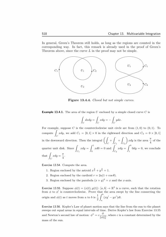
518 Chapter 13. Multivariable Integration
In general, Green’s Theorem still holds, as long as the regions are counted in thecorresponding way. In fact, this remark is already used in the proof of Green’sTheorem above, since the curve L in the proof may not be simple.
C2C1 U1
U2
C1
C2
U1
U2
Figure 13.4.4. Closed but not simple curves.
Example 13.4.1. The area of the region U enclosed by a simple closed curve C is∫U
dxdy =
∫C
xdy = −∫C
ydx.
For example, suppose C is the counterclockwise unit circle arc from (1, 0) to (0, 1). To
compute
∫C
xdy, we add C1 = [0, 1] × 0 in the rightward direction and C2 = 0 × [0, 1]
in the downward direction. Then the integral
(∫C
+
∫C1
+
∫C2
)xdy is the area
π
4of the
quarter unit disk. Since
∫C1
xdy =
∫ 1
0
xd0 = 0 and
∫C2
xdy =
∫ 0
1
0dy = 0, we conclude
that
∫C
xdy =π
4.
Exercise 13.54. Compute the area.
1. Region enclosed by the astroid x32 + y
32 = 1.
2. Region enclosed by the cardioid r = 2a(1 + cos θ).
3. Region enclosed by the parabola (x+ y)2 = x and the x-axis.
Exercise 13.55. Suppose φ(t) = (x(t), y(t)) : [a, b] → R2 is a curve, such that the rotationfrom φ to φ′ is counterclockwise. Prove that the area swept by the line connecting the
origin and φ(t) as t moves from a to b is1
2
∫ b
a
(xy′ − yx′)dt.
Exercise 13.56. Kepler’s Law of planet motion says that the line from the sun to the planetsweeps out equal areas in equal intervals of time. Derive Kepler’s law from Exercise 13.55
and Newton’s second law of motion: φ′′ = cφ
‖φ‖32, where c is a constant determined by the
mass of the sun.

13.4. Green’s Theorem 519
Exercise 13.57. Extend integration by parts by finding a relation between
∫U
(ufx+vgy)dxdy
and
∫U
(uxf + vyg)dxdy.
Exercise 13.58. The divergence of a vector field F = (f, g) on R2 is
divF = fx + gy.
Prove that ∫C
F · ~nds =
∫U
divFdA,
where ~n is the outward normal vector pointing away from U .
Exercise 13.59. The Laplacian of a two variable function f is ∆f = fxx + fyy = div∇f .Prove Green’s identities∫
U
f∆gdA =
∫C
f∇g · ~nds−∫U
∇f · ∇gdA,
and ∫U
(f∆g − g∆f)dA =
∫C
(f∇g − g∇f) · ~nds.
Potential: Antiderivative on R2
If fy = gx on a region U ⊂ R2 and C is the boundary curve, then Green’s Theorem
tells us
∫C
fdx+gdy = 0. The conclusion can be interpreted and utilized in different
ways.
Theorem 13.4.2. Suppose f and g are continuous functions on an open subsetU ⊂ R2. Then the following are equivalent.
1. The integral
∫C
fdx+ gdy along an oriented rectifiable curve C in U depends
only on the beginning and end points of C.
2. There is a differentiable function ϕ on U , such that ϕx = f and ϕy = g.
Moreover, if U is simply connected and f and g are continuously differentiable, thenthe above is also equivalent to
3. fy = gx on U .
The reason for the second statement to imply the first already appeared inExamples 13.1.6. Suppose f = ϕx and g = ϕy for differentiable ϕ, and C isparameterized by differentiable φ(t) = (x(t), y(t)), t ∈ [a, b]. Then∫
C
fdx+ gdy =
∫ b
a
(ϕxx′ + ϕyy
′)dt =
∫ b
a
dϕ(φ(t))
dtdt = ϕ(φ(b))− ϕ(φ(a)).
520 Chapter 13. Multivariable Integration
The right side depends only on the beginning point φ(a) and the end point φ(b) ofthe curve. For the proof in case C is only rectifiable, see Exercise 13.65.
To prove the converse that the first statement implies the second, we notethat f = ϕx and g = ϕy means that the vector field (f, g) is the gradient ∇ϕ.It also means that the 1-form fdx + gdy is the differential dϕ. The function ϕ,called a potential of the vector field (f, g) or the 1-form fdx + gdy, is actually thetwo-variable antiderivative of the vector field or the 1-form.
On R1, any continuous single variable function f(x) has antiderivative
ϕ(x) =
∫ x
a
f(t)dt.
On R2, we may imitate the single variable case and define
ϕ(x, y) =
∫ (x,y)
(a,b)
fdx+ gdy. (13.4.1)
The problem is that the integral should be along a path connecting (a, b) to (x, y),but there are many choices of such paths. In contrast, the integral for the singlevariable case is simply over the interval [a, x], the “unique path” connecting the twopoints.
Now we understand that the first statement of Theorem 13.4.2 means exactlythat the function (13.4.1) is well defined. It remains to show that the functionsatisfies ϕx = f and ϕy = g. Specifically, we will prove that
L(x, y) = ϕ(x0, y0) + f(x0, y0)(x− x0) + g(x0, y0)(y − y0)
is the linear approximation of ϕ near (x0, y0) ∈ U . By the continuity of f and g andthe openness of U , for any ε > 0, we can find δ > 0, such that ‖(x, y)−(x0, y0)‖2 < δimplies (x, y) ∈ U and ‖(f(x, y), g(x, y)) − (f(x0, y0), g(x0, y0))‖2 < ε. For such(x, y), let C be a path in U connecting (a, b) to (x0, y0) and let I be the straightline I connecting (x0, y0) to (x, y). Then
ϕ(x, y)− ϕ(x0, y0) =
(∫C∪I−∫C
)fdx+ gdy =
∫I
(fdx+ gdy).
Then we have
|ϕ(x, y)− L(x, y)| =∣∣∣∣∫I
(f(x, y)− f(x0, y0))dx+ (g(x, y)− g(x0, y0))dy
∣∣∣∣≤ sup
(x,y)∈I‖(f(x, y)− f(x0, y0), g(x, y)− g(x0, y0))‖2µ(I)
≤ ε‖(x, y)− (x0, y0)‖2.
Here the first inequality follows from Exercise 13.32. This proves the linear approx-imation.
Now we come to the third statement of Theorem 13.4.2. The third statementis a local property of f and g, because the partial derivatives depend only on the
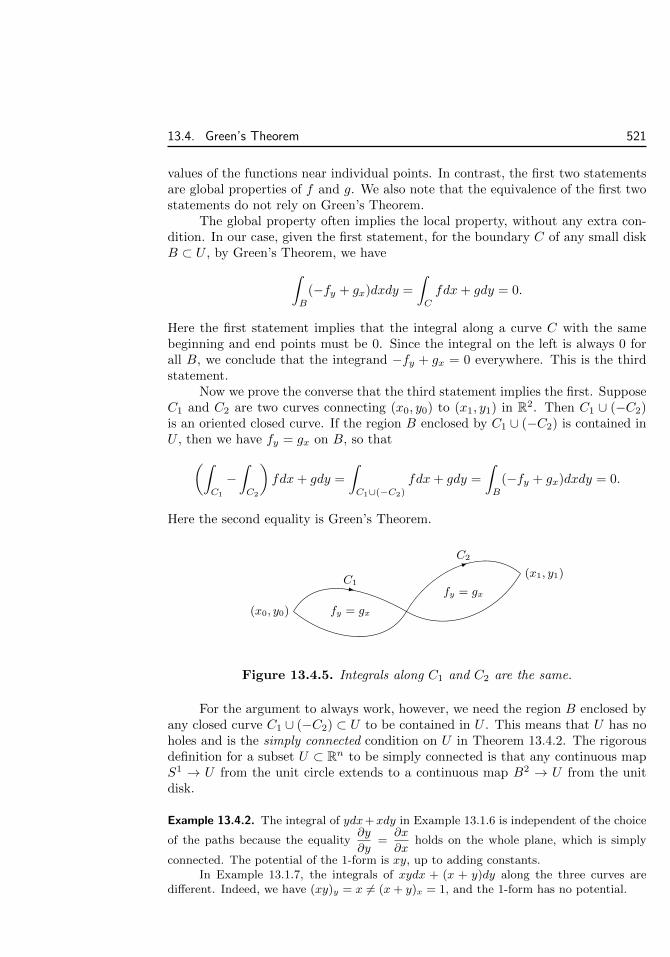
13.4. Green’s Theorem 521
values of the functions near individual points. In contrast, the first two statementsare global properties of f and g. We also note that the equivalence of the first twostatements do not rely on Green’s Theorem.
The global property often implies the local property, without any extra con-dition. In our case, given the first statement, for the boundary C of any small diskB ⊂ U , by Green’s Theorem, we have∫
B
(−fy + gx)dxdy =
∫C
fdx+ gdy = 0.
Here the first statement implies that the integral along a curve C with the samebeginning and end points must be 0. Since the integral on the left is always 0 forall B, we conclude that the integrand −fy + gx = 0 everywhere. This is the thirdstatement.
Now we prove the converse that the third statement implies the first. SupposeC1 and C2 are two curves connecting (x0, y0) to (x1, y1) in R2. Then C1 ∪ (−C2)is an oriented closed curve. If the region B enclosed by C1 ∪ (−C2) is contained inU , then we have fy = gx on B, so that(∫
C1
−∫C2
)fdx+ gdy =
∫C1∪(−C2)
fdx+ gdy =
∫B
(−fy + gx)dxdy = 0.
Here the second equality is Green’s Theorem.
(x0, y0)
(x1, y1)C1
C2
fy = gx
fy = gx
Figure 13.4.5. Integrals along C1 and C2 are the same.
For the argument to always work, however, we need the region B enclosed byany closed curve C1 ∪ (−C2) ⊂ U to be contained in U . This means that U has noholes and is the simply connected condition on U in Theorem 13.4.2. The rigorousdefinition for a subset U ⊂ Rn to be simply connected is that any continuous mapS1 → U from the unit circle extends to a continuous map B2 → U from the unitdisk.
Example 13.4.2. The integral of ydx+xdy in Example 13.1.6 is independent of the choice
of the paths because the equality∂y
∂y=
∂x
∂xholds on the whole plane, which is simply
connected. The potential of the 1-form is xy, up to adding constants.In Example 13.1.7, the integrals of xydx + (x + y)dy along the three curves are
different. Indeed, we have (xy)y = x 6= (x+ y)x = 1, and the 1-form has no potential.

522 Chapter 13. Multivariable Integration
Example 13.4.3. The vector field1
y2(xy2 + y, 2y − x) is defined on y > 0 and y < 0,
both simply connected. It satisfiesd
dy
(xy2 + y
y2
)= − 1
y2=
d
dx
(2y − xy2
). Therefore
it has a potential function ϕ. By ϕx =y(xy + 1)
y2, we get ϕ =
∫y(xy + 1)
y2dx + ϑ(y) =
x2
2+x
y+ ϑ(y). Then by ϕy = − x
y2+ ϑ′(y) =
2y − xy2
, we get ϑ′(y) =2
y, so that
ϑ(y) = 2 log |y|+ c. The potential function is
ϕ =x2
2+x
y+ 2 log |y|+ c.
In particular, we have∫ (2,2)
(1,1)
(xy2 + y)dx+ (2y − x)dy
y2=
(x2
2+x
y+ 2 log |y|
)(2,2)
(1,1)
=3
2+ log 2.
The example shows that the formula (13.4.1) may not be the most practical way ofcomputing the potential.
Example 13.4.4. The 1-formydx− xdyx2 + y2
satisfies
fy =
(y
x2 + y2
)y
=x2 − y2
(x2 + y2)2= gx =
(−x
x2 + y2
)x
on R2−(0, 0), which is unfortunately not simply connected. Let U be obtained by removingthe non-positive x-axis (−∞, 0] × 0 from R2. Then U is simply connected, and Theorem
13.4.2 can be applied. The potential forydx− xdyx2 + y2
is ϕ = −θ, where −π < θ < π is the
angle in the polar coordinate. The potential can be used to compute∫ (0,1)
(1,0)
ydx− xdyx2 + y2
= −θ(0, 1) + θ(1, 0) = −π2
+ 0 = −π2
for any curve connecting (1, 0) to (0, 1) that does not intersect the non-positive x-axis.
The unit circle arc C1 : φ1(t) = (cos t, sin t), 0 ≤ t ≤ π
2, and the straight line C2 : φ2(t) =
(1− t, t), 0 ≤ t ≤ 1, are such curves.On the other hand, consider the unit circle arc C3 : φ3(t) = (cos t,− sin t), 0 ≤ t ≤
3π
2, connecting (1, 0) to (0, 1) in the clockwise direction. To compute the integral along
the curve, let V be obtained by removing the non-negative diagonal (x, x) : x ≥ 0 fromR2. The 1-form still has the potential ϕ = −θ on V . The crucial difference is that the
range for θ is changed toπ
4< θ <
9π
4. Therefore∫ (0,1)
(1,0)
ydx− xdyx2 + y2
= −θ(0, 1) + θ(1, 0) = −π2
+ 2π =3π
2
for any curve connecting (1, 0) to (0, 1) that does not intersect the non-negative diagonal.
In general, the integral
∫ (0,1)
(1,0)
ydx− xdyx2 + y2
depends only on how the curve connecting
(1, 0) to (0, 1) goes around the origin, the only place where fy = gx fails.

13.4. Green’s Theorem 523
Exercise 13.60. Explain the computations in Exercise 13.25 by Green’s Theorem.
Exercise 13.61. Use potential function to compute the integral.
1.
∫C
2xdx+ ydy, C is the straight line connecting (2, 0) to (0, 2).
2.
∫C
xdx+ ydy
x2 + y2, C is the circular arc connecting (2, 0) to (0, 2).
3.
∫C
ydx− xdyax2 + by2
, C is the unit circle in counterclockwise direction.
4.
∫C
(x− y)dx+ (x+ y)dy
x2 + y2, C is the elliptic arc
x2
a2+y2
b2= 1 in the upper half plane
connecting (a, 0) to (−a, 0).
5.
∫C
(ex sin 2y − y)dx + (2ex cos 2y − 1)dy, C is the circular arc connecting (0, 1) to
(1, 0) in clockwise direction.
6.
∫C
(2xy3− 3y2 cosx)dx+ (−6y sinx+ 3x2y2)dy, C is the curve 2x = πy2 connecting
(0, 0) to(π
2, 1)
.
Exercise 13.62. Find p so that the vector fields(x, y)
(x2 + y2)pand
(−y, x)
(x2 + y2)phave potentials.
Then find the potentials.
Exercise 13.63. Compute the integral
∫C
g(xy)(ydx + xdy), where C is the straight line
connecting (2, 3) to (1, 6).
Exercise 13.64. Explain that the potential function is unique up to adding constants.
Exercise 13.65. We only proved that the second statement of Theorem 13.4.2 implies thefirst for the case that the curve C has differentiable parameterization. Extend the proof tothe case C is divided into finitely many segments, such that each segment has differentiableparameterization. Then further extend to general rectifiable C by using the idea of theproof of Theorem 13.4.1.
Integral Along Closed Curve
If fy = gx is satisfied, then the integral along a curve is “largely” dependent onlyon the end points. In fact, the value is only affected by the existence of holes, asillustrated by Example 13.4.4.
The open subset in Figure 13.4.6 has two holes, which are enclosed by simpleclosed curves C1 and C2 in U oriented in counterclockwise direction (opposite to thedirection adoptted in Green’s Theorem). The closed curve C in U may be dividedinto four parts, denoted C[1], C[2], C[3], C[4]. The unions of oriented closed curvesC[1]∪C[3]∪(−C1), C[2]∪(−C1), (−C[4])∪(−C2) also enclose subsets U1, U2, U3 ⊂ U .

524 Chapter 13. Multivariable Integration
If fy = gy on U , then by Green’s Theorem, we have(∫C[1]
+
∫C[3]
−∫C1
)fdx+ gdy =
∫C[1]∪C[3]∪(−C1)
fdx+ gdy
=
∫U1
(−fy + gx)dxdy = 0.
Similar argument can be made for the other two unions, and we get∫C[1]
+
∫C[3]
=
∫C1
,
∫C[2]
=
∫C1
,
∫C[4]
= −∫C2
.
Adding the three equalities together, we get∫C
fdx+ gdy =
(2
∫C1
−∫C2
)fdx+ gdy.
We remark that the coefficient 2 for C1 means that C wraps around C1 twice in thesame direction, and the coefficient −1 for C2 means that C wraps around C2 oncein the opposite direction.
C1
C2
U
C[1]
[2]
[3]
[4]
Figure 13.4.6. Closed curve in open subset with holes.
In general, suppose U has finitely many holes. We enclose these holes withclosed curves C1, . . . , Ck, all in counterclockwise orientation. Then any closed curveC in U wraps around the i-th hole ni times. The sign of ni is positive when thewrapping is counterclockwise (same as Ci) and is negative when the wrapping isclockwise (opposite to Ci). We say C is homologous to n1C1 + · · · + nkCk, and incase fy = gx on U , we have∫
C
fdx+ gdy =
(n1
∫C1
+ · · ·+ nk
∫Ck
)fdx+ gdy.
13.5. Stokes’ Theorem 525
Example 13.4.5. In Example 13.4.4, the 1-formydx− xdyx2 + y2
satisfies fy = gx on U =
R2− (0, 0). Since the unit circle C in the counterclockwise direction encloses the only holeof U , we have ∫
C
ydx− xdyx2 + y2
=
∫ 2π
0
sin t(− sin t)dt− cos t cos tdt
cos2 t+ sin2 t= −2π.
If C1 is a curve on the first quadrangle connecting (1, 0) to (0, 1) and C2 is a curve onthe second, third and fourth quadrangles connecting the two points, then C1 ∪ (−C2) ishomologous to C, and we have(∫
C1
−∫C2
)ydx− xdyx2 + y2
=
∫C
ydx− xdyx2 + y2
= −2π.
Therefore ∫C1
ydx− xdyx2 + y2
=
∫C2
ydx− xdyx2 + y2
− 2π.
Exercise 13.66. Study how the integral of the 1-formydx− xdyx2 + xy + y2
depends on the curves.
Exercise 13.67. Study how the integral of the 1-form
ω =(x2 − y2 − 1)dx+ 2xydy
((x− 1)2 + y2)((x+ 1)2 + y2)
depends on the curves. Note that if Cε is the counterclockwise circle of radius ε around
(1, 0), then
∫Cε0
ω = limε→0
∫Cε
ω.
13.5 Stokes’ TheoremGreen’s Theorem is the Fundamental Theorem of Calculus for 2-dimensional bodyin R2. The theorem can be extended to 2-dimensional surface in Rn.
2-Dimensional Fundamental Theorem of Calculus in R3
Let S ⊂ R3 be an oriented surface. Let
σ(u, v) = (x(u, v), y(u, v), z(u, v)) : U ⊂ R2 → S ⊂ R3
be an orientation compatible parameterization of S. Then the boundary C of Scorresponds to the boundary D of U . Recall that D should be oriented in such away that U is “on the left” of D. Correspondingly, C should also be oriented insuch a way that S is “on the left” of C.
The orientation of C can be characterized by the outward normal vector ~nout
along C, by requiring that the rotation from ~nout to the tangent vector ~t of C iscomparable to the rotation from σu to σv. Note that both ~nout,~t and σu, σv are

526 Chapter 13. Multivariable Integration
bases of the tangent space of S at boundary point. The same rotation requirementmeans that the matrix between the two bases has positive determinant, or
σu × σv = λ~nout × ~t, λ > 0.
Here λ is the determinant of the matrix for expressing σu, σv in terms of ~nout,~t.This is also equivalent to ~nout × ~t being the normal vector ~n of the surface S, andequivalent to det(~nout σu σv) > 0.
~t
~nout
UD
R2 : (u, v)
σ
~n
~t
~noutS
C
R3 : (x, y, z)
Figure 13.5.1. Boundary orientation compatible with the outward normal vector.
If F = (f, g, h) is a continuously differentiable vector field on R3, then∫C
fdx+ gdy + hdz =
∫D
(fxu + gyu + hzu)du+ (fxv + gyv + hzv)dv
=
∫U
((fxv + gyv + hzv)u − (fxu + gyu + hzu)v)dudv
=
∫U
(fuxv − fvxu + guyv − gvyu + huzv − hvzu)dudv.
The first equality is due to∫C
fdx =
∫ b
a
f(x(t), y(t), z(t))x′(t)dt
=
∫ b
a
f(x, y, z)(xuu′(t) + yuu
′(t))dt
=
∫D
fxudu+ fxvdv,
and the similar equalities for
∫C
gdy and
∫C
hdz. The second equality is Green’s
Theorem.By
fuxv − fvxu = (fxxu + fyyu + fzzu)xv − (fxxv + fyyv + fzzv)xu
= −fy det∂(x, y)
∂(u, v)+ fz det
∂(z, x)
∂(u, v),
13.5. Stokes’ Theorem 527
we have∫U
(fuxv − fvxu)dudv =
∫U
−fy det∂(x, y)
∂(u, v)dudv + fz det
∂(z, x)
∂(u, v)dudv
=
∫S
−fydx ∧ dy + fzdz ∧ dx.
Combined with the similar equalities for g and h, we get the following result.
Theorem 13.5.1 (Stokes’ Theorem). Suppose S ⊂ R3 is an oriented surface withcompatibly oriented boundary curve C. Then for any continuously differentiable f ,g, h along S, we have∫C
fdx+ gdy + hdz =
∫S
(gx − fy)dx ∧ dy + (hy − gz)dy ∧ dz + (fz − hx)dz ∧ dx.
Using the symbol
∇ =
(∂
∂x,∂
∂y,∂
∂z
),
the gradient of a function f can be formally denoted as
gradf = ∇f =
(∂f
∂x,∂f
∂y,∂f
∂z
).
Define the curl of a vector field F = (f, g, h) to be
curlF = ∇× F =
(∂h
∂y− ∂g
∂z,∂f
∂z− ∂h
∂z,∂g
∂x− ∂f
∂y
).
Then Stokes’ Theorem can be written as∫C
F · d~x =
∫S
curlF · ~ndA.
Example 13.5.1. Suppose C is the circle given by x2 + y2 + z2 = 1 and x + y + z = r,with the counterclockwise orientation when viewed from the direction of the x-axis. We
would like to compute the integral
∫C
(ax + by + cz + d)dx. Let S be the disk given by
x2 + y2 + z2 ≤ 1 and x+ y + z = r, with the normal direction given by (1, 1, 1). Then by
Stokes’ Theorem and the fact that the radius of S is
√1− r2
3, we have∫
C
(ax+by+cz+d)dx =
∫S
−bdx∧dy+cdz∧dx =
∫S
1√3
(−b+c)dA =c− b√
3π
(1− r2
3
).
Example 13.5.2. Faraday observed that a changing magnetic field B induces an electricfield E. More precisely, Faraday’s induction law says that the rate of change of the flux ofthe magnetic field through a surface S is the negative of the integral of the electric fieldalong the boundary C of the surface S. The law can be summarised as the equality
−∫C
E · d~x =d
dt
∫S
B · ~ndA.

528 Chapter 13. Multivariable Integration
By Stokes’ Theorem, the left side is −∫S
curlE · ~ndA. Since the equality holds for any
surface S, we conclude the differential version of Faraday’s law
−curlE =∂B
∂t.
This is one of Maxwell’s equations for electromagnetic fields.
Exercise 13.68. Compute
∫C
y2dx+ (x+ y)dy + yzdz, where C is the ellipse x2 + y2 = 2,
x+ y + z = 2, with clockwise orientation as viewed from the origin.
Exercise 13.69. Suppose C is any closed curve on the sphere x2 +y2 + z2 = R2. Prove that∫C
(y2 + z2)dx+ (z2 + x2)dy + (x2 + y2)dz = 0. In general, what is the condition for f , g,
h so that
∫C
fdx + gdy + hdz = 0 for any closed curve C on any sphere centered at the
origin?
Exercise 13.70. Find the formulae for the curls of F +G, gF .
Exercise 13.71. Prove that curl(gradf) = ~0. Moreover, compute curl(curlF ).
Exercise 13.72. The electric field E induced by a changing magnetic field is also changingand follows Ampere’s law∫
C
B · d~x = µ0
∫S
J · ~ndA+ ε0µ0d
dt
∫S
E · ~ndA,
where J is the current density, and µ0, ε0 are some physical constants. Derive the differ-ential version of Ampere’s law, which is the other Maxwell’s equation for electromagneticfields.
2-Dimensional Fundamental Theorem of Calculus in Rn
The key to derive Stokes’ Theorem is to translate the integral along a surface in R3
to the integral on a 2-dimensional body in R2. The argument certainly works inRn.
Let S be an oriented surface given by an orientation compatible regular pa-rameterization σ(u, v) : U ⊂ R2 → Rn. For n > 3, the surface no longer has normalvectors that we can use to describe the orientation. Instead, the orientation isgiven by the parameterization itself. If the surface is covered by several parameter-izations, then the derivatives of the transition maps are required to have positivedeterminants.
The boundary C of S corresponds to the boundary D of U . The boundaryD is oriented in such a ways that U is on the left side of D. The orientation of Dgives the orientation of C.
The compatible orientation of C can also be described by using the outwardnormal vector ~nout along C. The orientation of C is represented by the tangent

13.5. Stokes’ Theorem 529
vector ~t. Both ~nout,~t and σu, σv are bases of the tangent space of S at boundarypoint. We require the direction of ~t to be chosen in such a way that the matrixbetween the two bases has positive determinant. In terms of the exterior product,this means
σu ∧ σv = λ~n ∧ ~t, λ > 0.
~t
~nout
σu
σv
S
C
~x
T~xS
Rn
Figure 13.5.2. Compatible orientation of the boundary curve of a surface.
For a continuously differentiable f , we have∫C
fdxj =
∫D
f
(∂xj∂u
du+∂xj∂v
dv
)=
∫U
(∂
∂u
(f∂xj∂v
)− ∂
∂v
(f∂xj∂u
))dudv
=
∫U
(∂f
∂u
∂xj∂v− ∂f
∂v
∂xj∂u
)dudv
=
∫U
((∑i
∂f
∂xi
∂xi∂u
)∂xj∂v−
(∑i
∂f
∂xi
∂xi∂v
)∂xj∂u
)dudv
=
∫U
∑i
∂f
∂xi
(∂xi∂u
∂xj∂v− ∂xi
∂v
∂xj∂u
)dudv
=
∫U
∑i6=j
∂f
∂xidet
∂(xi, xj)
∂(u, v)dudv
=
∫S
∑i 6=j
∂f
∂xidxi ∧ dxj .
This leads to the following formula.
Theorem 13.5.2 (Stokes’ Theorem). Suppose S is an oriented surface in Rn withcompatible oriented boundary curve C. Then for any continuously differentiable f1,. . . , fn along the surface, we have∫
C
∑j
fjdxj =
∫S
∑i<j
(∂fj∂xi− ∂fi∂xj
)dxi ∧ dxj .

530 Chapter 13. Multivariable Integration
Potential: Antiderivative on Rn
With the help of Stokes’ Theorem in Rn, Theorem 13.4.2 may be extended, withthe same proof.
Theorem 13.5.3. Suppose F = (f1, . . . , fn) is a continuous vector field on an opensubset U ⊂ Rn. Then the following are equivalent.
1. The integral
∫C
F ·d~x along an oriented rectifiable curve C in U depends only
on the beginning and end points of C.
2. There is a differentiable function ϕ on U , such that ∇ϕ = F .
Moreover, if any closed curve in U is the boundary of an orientable surface in U ,and F is continuously differentiable, then the above is also equivalent to
3.∂fj∂xi
=∂fi∂xj
for all i, j.
The function ϕ in the theorem is the potential (or antiderivative) of the vectorfield F or the 1-form ω = f1dx1 + · · ·+ fndxn = F · d~x, and may be given by
ϕ(~x) =
∫ ~x
~x0
F · d~x.
We note that ∇ϕ = F is the same as dϕ = F · d~x.A closed curve C is homologous to 0 in U if it is the boundary of an oriented
surface in U . Two oriented curves C1 and C2 in U with the same beginning andend points are homologous in U if the closed curve C1 ∩ (−C2) is homologous to 0.Stokes’ Theorem implies that, if the third statement is satisfied, then the integralof the 1-form along homologous curves are equal. The extra condition in Theorem13.5.3 says that any two oriented curves with the same beginning and end pointsare homologous, so that the third statement implies the first.
A special case of the extra condition is that the subset U is simply connected.This means that any continuous map S1 → U extends to a continuous map B2 → U ,so that we can choose the surface to be the disk in the extra condition.
Example 13.5.3. The vector field (f, g, h) = (yz(2x+y+z), zx(x+2y+z), xy(x+y+2z))satisfies
fy = gx = (2x+ 2y + z)z, hy = gz = (x+ 2y + 2z)x, fz = hx = (2x+ y + 2z)y,
on the whole R3. Therefore the vector field has a potential, which can be computed byintegrating along successive straight lines connecting (0, 0, 0), (x, 0, 0), (x, y, 0), (x, y, z).The integral is zero on the first two segments, so that
ϕ(x, y, z) =
∫ z
0
xy(x+ y + 2z)dz = xyz(x+ y + z).

13.5. Stokes’ Theorem 531
Example 13.5.4. The 1-form x1 · · ·xn(dx1
x1+ · · ·+ dxn
xn
)satisfies
fi = x1 · · · xi · · ·xn,∂fj∂xi
= x1 · · · xi · · · xj · · ·xn
on the whole Rn. Therefore the 1-form has a potential. The potential function can beobtained by solving the system of equations
∂ϕ
∂xi= x1 · · · xi · · ·xn, i = 1, . . . , n.
The solution of the first equation is
ϕ = x1 · · ·xn + ψ(x2, . . . , xn).
Substituting into the other equations, we get
∂ϕ
∂xi= x1 · · · xi · · ·xn +
∂ψ
∂xi= x1 · · · xi · · ·xn, i = 2, . . . , n.
Thus we conclude that ψ is a constant, and x1 · · ·xn is a potential function of the 1-form.Solving the system of equations is actually the same as integrating along straight
lines in coordinate directions like Example 13.5.3. Alternatively, we may also use the lineintegral to compute the potential function. We have already verified that the line integraldepends only on the end points, and we may choose to integrate along the straight lineγ(t) = t~x connecting ~0 to ~x
ϕ(~x) =
∫ 1
0
n∑i=1
(tx1) · · · (txi) · · · (txn)(txi)
dtdt
=
∫ 1
0
n∑i=1
tn−1x1 · · ·xndt = x1 · · ·xn∫ 1
0
ntn−1dt = x1 · · ·xn.
Exercise 13.73. Determine whether the integral of vector field or the 1-form is independentof the choice of the curves. In the independent case, find the potential function.
1. ex(cos yz,−z sin yz,−y sin yz).
2. y2z3dx+ 2xyz3dy + 2xyz2dz.
3. (y + z)dx+ (z + x)dy + (x+ y)dz.
4. (x2, x3, . . . , xn, x1).
5. (x21, . . . , x
2n).
6. x1x2 · · ·xn(x−11 , . . . , x−1
n ).
Exercise 13.74. Explain that the potential function is unique up to adding constants.
Exercise 13.75. In R3, explain that Theorem 13.5.3 tells us that, if all closed curves in Uare homologous to 0, then F = gradϕ for some ϕ on U if and only if curlF = ~0 on U .
Exercise 13.76. Suppose ~a is a nonzero vector. Find condition on a function f(~x) so thatthe vector field f(~x)~a has a potential function.
Exercise 13.77. Find condition on a function f(~x) so that the vector field f(~x)~x has apotential function.

532 Chapter 13. Multivariable Integration
Exercise 13.78. Study the potential function of(y − z)dx+ (z − x)dy + (x− y)dz
(x− y)2 + (y − z)2.
Exercise 13.79. Suppose a continuously second order differentiable function g(~x) satisfies∇g(~x0) 6= ~0. Suppose f(~x) is continuously differentiable near ~x0. Prove that the differentialform
fdg = fgx1dx1 + fgx2dx2 + · · ·+ fgxndxn
has a potential near ~x0 if and only if f(~x) = h(g(~x)) for a continuously differentiable h(t).
13.6 Gauss’ TheoremGreen’s Theorem is the Fundamental Theorem of Calculus for 2-dimensional bodyin R2. The theorem can be extended to n-dimensional body in Rn.
3-Dimensional Fundamental Theorem of Calculus in R3
The key step in the proof of Green’s Theorem is to verify the case that U is theregion between two functions. In R3, consider the 3-dimensional region betweencontinuously differentiable functions h(x, y) and k(x, y) on V ⊂ R2
U = (x, y, z) : (x, y) ∈ V, k(x, y) ≤ z ≤ h(x, y).
The boundary surface S of U is oriented to be compatible with the outward normalvector ~nout.
St
Sb
~nout
~nout
~nout
z = h(x, y)
z = k(x, y) Sv
U
V
Figure 13.6.1. Gauss’ Theorem for a special case.

13.6. Gauss’ Theorem 533
We have∫U
fzdxdydz =
∫V
(∫ h(x,y)
k(x,y)
fz(x, y, z)dz
)dxdy (Fubini Theorem)
=
∫V
(f(x, y, h(x, y))− f(x, y, k(x, y)))dxdy. (Fundamental Th.)
On the other hand, the boundary surface S of U consists of three pieces. The toppiece St is usually parameterized by
σ(x, y) = (x, y, h(x, y)), (x, y) ∈ V.
By the computation in Example 13.2.6, the parameterization is compatible with thenormal vector
~n =(−fx,−fy, 1)√f2x + f2
y + 1.
Since ~n points upwards (the third coordinate is positive) and therefore outwards,we get ~n = ~nout. Therefore the parameterization is compatible with the orientationof the top piece, and we have∫
St
fdx ∧ dy =
∫V
f(σ(x, y))dxdy =
∫V
f(x, y, h(x, y))dxdy.
The bottom piece Sb is usually parameterized by
σ(x, y) = (x, y, k(x, y)), (x, y) ∈ V.
The parameterization is also compatible with the upward normal vector. Since theoutward normal vector of the bottom piece points downward (the third coordinateis negative), we get ~n = −~nout for Sb, so that∫
Sb
fdx ∧ dy = −∫V
f(x, y, k(x, y))dxdy.
We also have the usual parameterization of the side piece Sv
σ(t, z) = (x(t), y(t), z), k(x, y) ≤ z ≤ h(x, y),
where (x(t), y(t)) is a parameterization of the boundary curve of V . Then∫Sv
fdx ∧ dy = ±∫a≤t≤b,k(x,y)≤z≤h(x,y)
f(x(t), y(t), z) det∂(x, y)
∂(t, z)dtdz = 0.
We conclude that∫S
fdx ∧ dy =
(∫St
+
∫Sb
+
∫Sv
)fdx ∧ dy
=
∫V
f(x, y, h(x, y))dxdy −∫V
f(x, y, k(x, y))dxdy
=
∫U
fzdxdydz.

534 Chapter 13. Multivariable Integration
For a more general region U ⊂ R3, we may use the idea of the proof of Green’sTheorem. In other words, we divide U into several special regions between graphsof functions and add the equality above for each region to get the same equality for
U . Similar equalities for
∫S
gdy∧dz and
∫S
hdz∧dx can be established by rotating
x, y and z.
Theorem 13.6.1 (Gauss’ Theorem). Suppose U ⊂ R3 is a region with the boundarysurface S compatibly oriented with respect to the outward normal vector. Then forany continuously differentiable f , g, h, we have∫
S
fdy ∧ dz + gdz ∧ dx+ hdx ∧ dy =
∫U
(fx + gy + hz)dxdydz.
Define the divergence of a vector field F = (f, g, h) to be
divF = ∇ · F =∂f
∂x+∂g
∂y+∂h
∂z.
Then Gauss’ Theorem means that the outward flux of a flow F = (f, g, h) is equalto the integral of the divergence of the flow on the solid∫
S
F · ~ndA =
∫U
divFdV.
Example 13.6.1. The volume of the region enclosed by a surface S ⊂ R3 without boundaryis ∫
S
xdy ∧ dz =
∫S
ydz ∧ dx =
∫S
zdx ∧ dy =1
3
∫S
(x, y, z) · ~ndA.
Example 13.6.2. In Example 13.2.9, the outgoing flux of the flow F = (x2, y2, z2) through
the ellipse(x− x0)2
a2+
(y − y0)2
b2+
(z − z0)2
c2= 1 is computed by surface integral. Alter-
natively, by Gauss’ theorem, the flux is∫F · ~ndA =
∫(x−x0)2
a2+
(y−y0)2
b2+
(z−z0)2
c2≤1
2(x+ y + z)dxdydz
=
∫x2
a2+ y2
b2+ z2
c2≤1
2(x+ x0 + y + y0 + z + z0)dxdydz.
By the transform ~x→ −~x, we get∫x2
a2+ y2
b2+ z2
c2≤1
(x+ y + z)dxdydz = 0.
Therefore the flux is∫x2
a2+ y2
b2+ z2
c2≤1
2(x0 + y0 + z0)dxdydz =8πR3
3abc(x0 + y0 + z0).

13.6. Gauss’ Theorem 535
Example 13.6.3. To compute the upward flux of F = (xz,−yz, (x2 + y2)z) through thesurface S given by 0 ≤ z = 4− x2− y2, we introduce the disk D = (x, y, 0) : x2 + y2 ≤ 4on the (x, y)-plane. Taking the normal direction of D to be (0, 0, 1), the surface S ∪ (−D)is the boundary of the region U given by 0 ≤ z ≤ 4 − x2 − y2. By Gauss’ theorem, theflux through S is∫
S
F · ~ndA =
∫S∪(−D)
F · ~ndA+
∫D
F · ~ndA
=
∫U
(z − z + x2 + y2)dxdydz +
∫x2+y2≤4
F (x, y, 0) · (0, 0, 1)dA
=
∫U
(x2 + y2)dxdydz =
∫0≤r≤2,0≤θ≤2π
r2(4− r2)rdrdθ =32π
3.
Example 13.6.4. The gravitational field created by a mass M at point ~x0 ∈ R is
G = − M
‖~x− ~x0‖32(~x− ~x0).
A straightforward computation shows divG = 0. Suppose U is a region with compatiblyoriented boundary surface S and ~x0 6∈ S. If ~x0 6∈ U , then by Gauss’ theorem, the outward
flux
∫S
G · ~ndA = 0. If ~x0 ∈ U , then let Bε be the ball of radius ε centered at ~x0. The
boundary of the ball is the sphere Sε, which we given an orientation compatible with the
outward normal vector ~n =~x− ~x0
‖~x− ~x0‖2. For sufficiently small ε, the ball is contained in
U . Moreover, U −Bε is a region not containing ~x0 and has compatibly oriented boundarysurface S ∪ (−Sε). Therefore∫S
G · ~ndA =
∫Sε
G · ~ndA =
∫‖~x−~x0‖2=ε
−Mε3
(~x− ~x0) · ~x− ~x0
εdA = −M
ε2
∫Sε
dA = −4πM.
More generally, the gravitational field created by several masses at various locationsis the sum of the individual gravitational field. The outward flux of the field through S isthen −4π multiplied to the total mass contained in A. In particular, the flux is independentof the specific location of the mass, but only on whether the mass is inside A or not. Thisis called Gauss’ Law.
Exercise 13.80. Compute the flux.
1. Outward flux of (x3, x2y, x2z) through boundary of the solid x2 +y2 ≤ a2, 0 ≤ z ≤ b.
2. Inward flux of (xy2, yz2, zx2) through the ellipse(x− x0)2
a2+
(y − y0)2
b2+
(z − z0)2
c2=
1.
3. Upward flux of (x3, y3, z3) through the surface z = x2 + y2 ≤ 1.
4. Outward flux of (x2, y2,−2(x+ y)z) through the torus in Example 8.1.17.
Exercise 13.81. Suppose U ⊂ R3 is a convex region with boundary surface S. Suppose ~ais a vector in the interior of U , and p is the distance from ~a to the tangent plane of S.
Compute
∫S
pdA. Moreover, for the special case S is the ellipsex2
a2+y2
b2+z2
c2= 1 and
~a = (0, 0, 0), compute
∫S
1
pdA.

536 Chapter 13. Multivariable Integration
Exercise 13.82. Find the formulae for the divergences of F +G, gF , F ×G.
Exercise 13.83. Prove that div(curlF ) = 0. Moreover, compute div(gradf) and grad(divF ).
Exercise 13.84. Find all the functions f on R3, such that the integral of the differentialform fdy ∧ dz + zdx ∧ dy on any sphere is 0.
n-Dimensional Fundamental Theorem of Calculus in Rn
Such a fundamental theorem is inevitable, and the proof is routine. First we considerthe special region
U = (~u, xn) : ~u ∈ V, k(~u) ≤ xn ≤ h(~u), ~u = (x1, . . . , xn−1).
The boundary S of U is oriented to be compatible with the outward normal vector~nout.
By Fubini Theorem and the classical Fundamental Theorem of Calculus, wehave ∫
U
fxndx1 · · · dxn =
∫V
(f(~u, h(~u))− f(~u, k(~u)))dx1 · · · dxn−1.
By the computation in Example 13.3.3, the usual parameterizations of the top pieceSt
σ(~u) = (~u, h(~u)), ~u ∈ V,and the bottom piece Sb
σ(~u) = (~u, k(~u)), ~u ∈ V,
are compatible with the normal vector with last coordinate having sign (−1)n−1.Since the ~nout has positive last coordinate on St and negative last coordinate onSb, we get∫
St
fdx1 ∧ · · · ∧ dxn−1 = (−1)n−1
∫V
f(~u, h(~u))dx1 · · · dxn−1, (13.6.1)∫Sb
fdx1 ∧ · · · ∧ dxn−1 = (−1)n∫V
f(~u, k(~u))dx1 · · · dxn−1. (13.6.2)
Similar to the earlier discussions, we also have∫Sv
fdx1 ∧ · · · ∧ dxn−1 = 0.
Then we get ∫S
(−1)n−1fdx1 ∧ · · · ∧ dxn−1 =
∫U
fxndx1 · · · dxn.
By the same argument, especially using the computations in Example 13.3.3and Exercise 13.49, we get∫
S
(−1)i−1fdx1 ∧ · · · ∧ dxi ∧ · · · ∧ dxn =
∫U
fxidx1 · · · dxn.

13.7. Additional Exercise 537
Theorem 13.6.2 (Gauss’ Theorem). Suppose U ⊂ Rn is a region with the boundarysubmanifold S compatibly oriented with respect to the outward normal vector. Thenfor any continuously differentiable f1, . . . , fn, we have∫
S
∑(−1)i−1fidx1 ∧ · · · ∧ dxi ∧ · · · ∧ dxn =
∫U
(∂f1
∂x1+ · · ·+ ∂fn
∂xn
)dx1 · · · dxn.
If we define the divergence of a vector field on Rn to be
divF =∂f1
∂x1+ · · ·+ ∂fn
∂xn.
then Gauss’ Theorem can be rewritten as∫S
F · ~ndV =
∫U
divFdµ~x.
We obtained Stokes’ Theorems 13.5.1 and 13.5.2 by “transferring” Green’sTheorem to a surface in Rn. By the same method, we can “transfer” Gauss’ The-orems 13.6.1 and 13.6.2 to submanifolds of higher dimensional Euclidean spaces.However, we will leave the discussion to the next chapter, because there is anotherdeep insight that the high dimensional Fundamental Theorems of Calculus does notrequire Euclidean space at all!
13.7 Additional ExerciseGauss Map
Let M be an oriented submanifold of Rn of dimension n − 1. The normal vector can beconsidered as a map ν = ~n : M → Sn−1 ⊂ Rn, called the Gauss map.
Exercise 13.85. Prove that the derivative ν′ maps T~xM to the subspace T~xM ⊂ Rn. Themap ν′ : T~xM → T~xM is called the Weingarten map.
Exercise 13.86. Prove that the Weingarten map is self-adjoint: ν′(~u) · ~v = ~u · ν′(~v) for any~u,~v ∈ T~xM .
Exercise 13.87. Compute the Weingarten map.
1. M = ~x : ~a · ~x = c is a hyperplane of Rn.
2. M = Sn−1R is the sphere of radius R in Rn.
3. M = Sn−2R × R is the cylinder of radius R in Rn.
Principal Curvatures
For an oriented submanifold M of Rn of dimension n− 1, its thickening map
φ(~x, t) = ~x+ t~n(~x) : M × [a, b]→ Rn,
is injective for small a, b and describes an open neighborhood N[a,b] of M in Rn in casea < 0 < b.

538 Chapter 13. Multivariable Integration
Let σ : U → M is an orientation compatible parameterization of M . Let W be thematrix of the Weingarten map with respect to the basis σu1 , . . . , σun−1 . Then
det(I + tW ) = 1 + t(n− 1)H1 + · · ·+ tk(n− 1)!
(k − 1)!(n− k)!Hk−1 + · · ·+ tn−1Hn−1.
We call H1 the mean curvature and call Hn−1 the Gaussian curvature.
Exercise 13.88. Explain that Hk are independent of the choice of the parameterization σ.
Exercise 13.89. Prove that ‖φu1 ∧ · · · ∧ φun−1 ∧ φt‖2 = det(I + tL)‖σu1 ∧ · · · ∧ σun−1‖2 forsmall t.
Exercise 13.90. Prove that the volume of N[0,b] is
bVol(M) +n− 1
2b2∫M
H1dV + · · ·+ (n− 1)!
k!(n− k)!bk∫M
HkdV + · · ·+ 1
nbn∫M
Hn−1dV.
What about the volumes of N[a,0] and N[a,b]?
Exercise 13.91. Derive the formula in Example 13.3.1.

Chapter 14
Manifold
539

540 Chapter 14. Manifold
14.1 ManifoldIn Section 8.4, we defined an n-dimensional submanifold of RN to be a subsetM ⊂ RN , such that near any point in M , the subset is the graph of a continuouslydifferentiable map f of some choice of N − n coordinates ~z in terms of the othern coordinates ~y. Specifically, if vectors of RN are written as ~x = (~y, ~z), ~y ∈ Rn,~z ∈ RN−n, then
ϕ(~y) = (~y, f(~y)) : U →M
is a regular parameterization near the point, in the sense that the partial derivativeof ϕ in ~y is invertible. Conversely, by Proposition 8.4.2, a submanifold of RN is asubset M , such that there is a regular parameterization near any point of M .
Another motivation for differentiable manifolds is from the discussion leadingto the definition (??) of the integral of a form on an oriented surface. The discussionsuggests that the integral can be defined as long as there are orientation compatibleparameterizations of pieces of the surface. The key observation is that the ambientEuclidean space RN is not needed in the definition of the integral.
Differentiable Manifold
The following is the preliminary definition of differentiable manifolds. The rigorousdefinition requires extra topological conditions and will be given in Definition 14.2.10after we know more about the topology of manifolds.
Definition 14.1.1 (Preliminary). A differentiable manifold of dimension n is a setM and a collection of injective maps
σi : Ui →Mi = σi(Ui) ⊂M,
such that the following are satisfied.
1. M is covered by Mi: M = ∪Mi.
2. Ui are open subsets of Rn.
3. Uij = σ−1i (Mi ∩Mj) are open subsets of Rn.
4. The transition maps ϕji = σ−1j σi : Uij → Uji are continuously differentiable.
If the transition maps are r-th order continuously differentiable, then we sayM is an r-th order differentiable manifold, or Cr-manifold. If the transition mapsare continuously differentiable of any order, then M is a smooth manifold, or C∞-manifold. On the other hand, if the transition maps are only continuous, then Mis a topological manifold, or C0-manifold.
The map σi is a (coordinate) chart. A collection σi of coordinate chartssatisfying the conditions of the definition is an atlas of the manifold. The samemanifold may allow different choices of atlases. For example, any way of expressingthe circle as a union of some open circular intervals gives an atlas of the circle.On the other hand, the concept of manifold should be independent of the choice

14.1. Manifold 541
M
Uij ϕji
Uji
Ui
σi
Mi
Uj
σj
Mj
Figure 14.1.1. Transition map between overlapping parameterizations.
of atlas. To solve the problem of dependence on the atlas, we say an injectionσ : U → σ(U) ⊂M from an open subset U ⊂ Rn is a (compatible) chart if for eachexisting chart σi, σ
−1i (Mi ∩ σ(U)) is an open subset of Ui, and the map
σ−1 σi : σ−1i (Mi ∩ σ(U))→ U
is continuously differentiable. A unique atlas of a manifold can then be constructedby including all the compatible charts to form the maximal atlas.
Example 14.1.1. Any open subset U ⊂ Rn is a manifold. We can simply use the identitymap U → U as an atlas. Any other chart is simply an injective continuously differen-tiable map σ : V ⊂ Rn → U from an open subset V ⊂ Rn, such that σ(V ) is open, andσ−1 : σ(V )→ V is also continuously differentiable.
Example 14.1.2. In Example 8.4.4, the unit circle S1 = (x, y) : x2 + y2 = 1 has reg-ular parameterizations given by expressing one coordinate as the function of the othercoordinate
σ1(u) = (u,√
1− u2) : U1 = (−1, 1)→M1 ⊂ S1,
σ−1(u) = (u,−√
1− u2) : U−1 = (−1, 1)→M−1 ⊂ S1,
σ2(u) = (√
1− u2, u) : U2 = (−1, 1)→M2 ⊂ S1,
σ−2(u) = (−√
1− u2, u) : U−2 = (−1, 1)→M−2 ⊂ S1.
Here M1,M−1,M2,M−2 are respectively the upper, lower, right, and left half circles.The overlapping M1 ∩M2 is the upper right quarter of the circle. The transition mapϕ21(u) = σ−1
2 σ1(u) = w is obtained by solving σ1(u) = σ2(w), or (∗,√
1− u2) = (∗, w).Therefore
ϕ21(u) =√
1− u2 : U12 = (0, 1)→ U21 = (0, 1).
We can similarly get the other three transition maps, such as
ϕ(−2)1(u) =√
1− u2 : U1(−2) = (−1, 0)→ U(−2)1 = (0, 1).

542 Chapter 14. Manifold
All transition maps are smooth.
Example 14.1.3. Consider the sphere Sn of radius1
2(or diameter 1). Fixing two antipodal
points N and S as the north and south poles, we have the stereographical projection fromthe north pole
σN (~u) = ξ : Rn → Sn − N.The chart misses the north pole. To cover the whole sphere, we also need to use thestereographical projection from the south pole
σS(~v) = ξ : Rn → Sn − S.
ξ
N
1
S
~v
~u
Rn
Rn
N
1
S
~v
~u
ξ
Figure 14.1.2. Stereographic projections.
The overlapping of the two charts is Sn − N,S, and
UNS = σ−1N (Sn − N,S) = Rn −~0, USN = σ−1
S (Sn − N,S) = Rn −~0.
The transition map is
ϕNS(~u) = σ−1N σS(~u) = ~v : Rn −~0→ Rn −~0.
Note that by the obvious identification of the two Rn (explicitly given by (x1, . . . , xn,12)↔
(x1, . . . , xn,− 12)), ~u and ~v point to the same direction, and their Euclidean lengths are
related by ‖~u‖2‖~v‖2 = 12 = 1. Therefore we get
ϕNS(~v) =~v
‖~v‖22.
The transition map is smooth.
Example 14.1.4 (Open Mobius Band). Let Lθ be the line passing through the point z(θ) =(cos θ, sin θ) on the unit circle at angle θ and with slope 1
2θ. The Mobius band is
M = (z, v) : z ∈ S1, v ∈ Lθ.
Although all Lθ intersect at v = (−1, 0), we consider (z, v) and (z′, v) to be different pointsof M if z 6= z′. On the other hand, if z(θ) = z(θ′), then θ− θ′ is an integer multiple of 2π,and Lθ and Lθ′ are the same line. So there is no ambiguity in the definition of M .

14.1. Manifold 543
Lθ
z
v
θ2 θ
Figure 14.1.3. Open Mobius band.
Corresponding to the covering of the circle by two charts (0, 2π) and (−π, π), wehave two charts for the Mobius band, given by the same formula
σi(θ, t) = ((cos θ, sin θ), (cos θ, sin θ) + t(cos 12θ, sin 1
2θ)),
but with different domain
σ0 : U0 = (0, 2π)× R→M, σ1 : U1 = (−π, π)× R→M.
The transition map ϕ10(θ, t) = (θ′, t′) on the overlapping (0, π)×Rt(π, 2π)×R is obtainedby solving σ0(θ, t) = σ1(θ′, t′). The solution consists of two parts
ϕ+10(θ, t) = (θ, t) : (0, π)× R→ (0, π)× R,
ϕ−10(θ, t) = (θ − 2π,−t) : (π, 2π)× R→ (−π, 0)× R.
Both are smooth maps.
Example 14.1.5. The real projective space RPn is the set of the lines in Rn+1 passingthrough the origin. Such a line is a 1-dimensional subspace, and is spanned by a nonzerovector (x0, x1, . . . , xn). Denoting the span by [x0, x1, . . . , xn], we have
RPn = [x0, x1, . . . , xn] : some xi 6= 0.
If xi 6= 0, then (x0, x1, . . . , xn) and1
xi(x0, x1, . . . , xn) span the same subspace. This leads
to the injective maps
σi(x1, . . . , xn) = [x1, . . . , xi, 1, xi+1, . . . , xn] : Rn → RPn, 0 ≤ i ≤ n,
with the images Mi = [x0, x1, . . . , xn] : xi 6= 0.For the overlapping M0 ∩M1 = [x0, x1, . . . , xn] : x0 6= 0 and x1 6= 0, we have
U01 = U10 = (x1, . . . , xn) : x1 6= 0.
The transition map ϕ10(x1, x2, . . . , xn) = (y1, y2, . . . , yn) is obtained from
σ0(x1, . . . , xn) = [1, x1, x2, . . . , xn] = [y1, 1, y2, . . . , yn] = σ1(y1, . . . , yn).
Therefore
ϕ10(x1, x2 . . . , xn) =
(1
x1,x2
x1. . . ,
xnx1
).
We can get similar formulae for the other transition maps. All the transition maps aresmooth.

544 Chapter 14. Manifold
Example 14.1.6. The complex projective space CPn is the set of all complex 1-dimensionalsubspaces of Cn+1. Denoting by [z0, z1, . . . , zn] the complex subspace spanned by (nonzero)complex vector (z0, z1, . . . , zn), we have
CPn = [z0, z1, . . . , zn] : some zi 6= 0.
Like RPn, the complex projective space is also a manifold. We specifically look at CP 1,which like the real case is covered by two charts (w is a complex number)
σ0(w) = [1, w] : U0 = C→M0 = [z0, z1] : z0 6= 0,σ1(w) = [w, 1] : U1 = C→M1 = [z0, z1] : z1 6= 0.
The overlapping M0 ∩ M1 consists of those [z0, z1] with both z0 and z1 nonzero. Thetransition map is
ϕ10(w) =1
w: U01 = C− 0→ U10 = C− 0.
In terms of w = u+ iv, u, v ∈ R, the transition map is
ϕ10(u, v) =
(u
u2 + v2,−v
u2 + v2
): R2 − (0, 0)→ R2 − (0, 0).
Exercise 14.1. Show that the torus is a differentiable manifold by constructing an atlas.
Exercise 14.2. Show that the special linear group SL(2) in Example 8.4.9 is a differentiablemanifold by constructing an atlas.
Exercise 14.3. The points on the circle can be described by angles θ, with θ and θ + 2πcorresponding to the same point. Find the atlas consisting of two circle intervals (−δ, π+δ)and (−π − δ, δ), where 0 < δ < π. Find the transition map.
Exercise 14.4. Show that the two atlases of the circle in Example 14.1.2 and Exercises 14.3are compatible and therefore give the same manifold.
Exercise 14.5. In Example 14.1.3, find the formula of ξ in terms of ~u and ~v.
Exercise 14.6. Extend Example 14.1.2 to the unit sphere Sn in Rn+1. Then (after scalingby 2 to match radius 1
2) compare with the stereographical projection charts in Example
14.1.3.
Exercise 14.7. Describe the atlas of the circle given by the stereographical projection inExample 14.1.3. Then compare the atlas with the atlas of the real projective space RP 1
in Example 14.1.5. Explain why the circle and RP 1 are the same manifold.
Exercise 14.8. Show that the sphere S2 and the complex projective space CP 1 are the sameby comparing the stereographic projection atlas of S2 with the atlas of CP 1 in Example14.1.6.
Exercise 14.9. Describe an atlas for the complex projective space CPn.

14.1. Manifold 545
Exercise 14.10. Show that if we change1
2θ to
5
2θ in Example 14.1.4, then we still get the
Mobius band.
Exercise 14.11 (Klein Bottle). The Klein bottle is obtained by identifying the boundaries ofthe square [−1, 1]× [−1, 1] as follows
(x, 1) ∼ (−x,−1), (1, y) ∼ (−1, y).
Show that the Klein bottle is a differentiable manifold.
Exercise 14.12 (Mapping Torus). Let L be an invertible linear transform on Rn. Show thatthe mapping torus obtained by glueing two ends of Rn × [0, 1] by (~x, 1) ∼ (L(~x), 0) is adifferentiable manifold.
Exercise 14.13. Suppose M and N are manifolds of dimensions m and n. Prove that theproduct M×N is a manifold of dimension m+n. Specifically, prove that if σi : Ui →Miand τj : Vj → Nj are atlases of M and N , then σi× τj : Ui×Vj →Mi×Nj is an atlasof M ×N .
Exercise 14.14. Show that it is always possible to find an atlas of a differentiable manifold,such that every Ui = Rn.
Manifold with Boundary
Definitions 14.1.1 only gives manifolds without boundary. If we allow Ui and Uij tobe open subsets of either the whole Euclidean space Rn or the half Euclidean space
Rn+ = (u1, u2, . . . , un−1, un) : un ≥ 0,
then we get manifolds with boundary, and the boundary ∂M consists of those pointscorresponding to
∂Rn+ = (u1, u2, . . . , un−1, 0) = Rn−1 × 0.
In other words,∂M = ∪Ui⊂Rn+σi(Ui ∩ Rn−1 × 0).
In the extended definition, a subset of Rn+ is open if it is of the form Rn+ ∩ Ufor some open subset U of Rn. Moreover, a map on an open subset of Rn+ is(continuously) differentiable if it is the restriction of a (continuously) differentiablemap on an open subset of Rn. This makes it possible for us to talk about thedifferentiability of the transition maps between open subsets of Rn+.
Proposition 14.1.2. The boundary of an n-dimensional differentiable manifold isan (n− 1)-dimensional differentiable manifold without boundary.
Proof. An atlas for the boundary ∂M can be obtained by restricting an atlas of Mto Rn−1 × 0
τi = σi|Rn−1×0 : Vi = Ui ∩ Rn−1 × 0→ (∂M)i = σi(Ui ∩ Rn−1 × 0).

546 Chapter 14. Manifold
The transition maps between the charts τi are continuously differentiable becausethey are the restrictions of continuously differentiable transition maps of M (whichare again restrictions of continuously differentiable maps on open subsets of Rn).Moreover, ∂M has no boundary because Vi are open subsets of the whole Euclideanspace Rn−1 (the half space Rn−1
+ is not used for the atlas).
Example 14.1.7. The interval M = [0, 1] is covered by charts
σ1(t) = t : U1 = [0, 1)→M1 = [0, 1) ⊂M,
σ2(t) = 1− t : U2 = [0, 1)→M2 = (0, 1] ⊂M.
Here U1 = U2 = [0, 1) = (−1, 1) ∩ R+ are open subsets of the half line R+ = [0,+∞),and the transition map ϕ21(t) = 1 − t : (0, 1) → (0, 1) is continuously differentiable. Theboundary of the interval is
∂[0, 1] = σ1(0) ∪ σ2(0) = 0, 1.
Example 14.1.8. The disk M = (x, y) : x2 + y2 ≤ 1 is covered by charts
σ0(x, y) = (x, y) : U0 = (x, y) : x2 + y2 < 1 →M0 ⊂M,
σ1(r, θ) = (r cos θ, r sin θ) : U1 = (0, 1]× (−δ, π + δ)→M1 ⊂M,
σ2(r, θ) = (r cos θ, r sin θ) : U2 = (0, 1]× (−π − δ, δ)→M2 ⊂M.
Here we use Exercise 14.3 for the circular direction. Note that to make the formulae moremanageable, we relaxed the choice of Ui to be open subsets of any half Euclidean space,and the half plane used here is (−∞, 1]×R. If we insist on using the standard half space,then the charts have more cumbersome formulae
σ0(x, y) = (x, y) : U0 = (x, y) : x2 + y2 < 1 →M0 ⊂M,
σ1(θ, t) = ((1− t) cos θ, (1− t) sin θ) : U1 = (−δ, π + δ)× [0,+∞)→M1 ⊂M,
σ2(θ, t) = ((1− t) cos θ, (1− t) sin θ) : U2 = (−π − δ, δ)× [0,+∞)→M2 ⊂M.
We can easily find the transition maps
ϕ01(x, y) = (r cos θ, r sin θ) : U10 = (0, 1)× (−δ, π + δ)
→ U01 = (x, y) : 0 < x2 + y2 < 1,−δ < θ(x, y) < π + δ,ϕ02(x, y) = (r cos θ, r sin θ) : U20 = (0, 1)× (−π − δ, δ)
→ U02 = (x, y) : 0 < x2 + y2 < 1,−π − δ < θ(x, y) < δ,
ϕ21(r, θ) =
(r, θ) : (0, 1]× (−δ, δ)→ (0, 1]× (−δ, δ),(r, θ − 2π) : (0, 1]× (π − δ, π + δ)→ (0, 1]× (−π − δ,−π + δ).
These are continuously differentiable. Therefore the disk is a differentiable manifold, withthe unit circle as the boundary
∂M = σ1(0× (−δ, π + δ)) ∪ σ2((−π − δ, δ)) = (x, y) : x2 + y2 = 1.
The idea of the example can be extended to show that the ball in Rn is a manifoldwith the sphere Sn−1 as the boundary. See Exercise 14.16.

14.1. Manifold 547
Example 14.1.9 (Mobius band). Consider the circle γ(θ) = (cos θ, sin θ, 0) lying in the(x, y)-plane in R3. At each point γ(θ) of the circle, let Iθ be the interval that is perpen-
dicular to the circle, has angle1
2θ from the (x, y)-plane, has length 1 and has the point
γ(θ) as the center. Basically Iθ moves along the circle while rotating at half speed. Theunion M = ∪Iθ is the Mobius band.
To find an atlas for the Mobius band, we note that the direction of Iθ is
v(θ) =
(cos
1
2θ cos θ, cos
1
2θ sin θ, sin
1
2θ
).
Then we use Exercise 14.3 for the circular direction and get charts
σ1(θ, t) = γ(θ) + tv(θ), (θ, t) ∈ U1 = (−δ, π + δ)× [−0.5, 0.5],
σ2(θ, t) = γ(θ) + tv(θ), (θ, t) ∈ U2 = (−π − δ, δ)× [−0.5, 0.5].
Here we further relaxed the choice of Ui compared with Example 14.1.8, again to makeour formulae more manageable. Strictly speaking, we should split σ1 into two charts
σ1+(θ, t) = σ1(θ, t− 0.5), σ1−(θ, t) = σ1(θ, 0.5− t), (θ, t) ∈ (−δ, π + δ)× [0, 1),
and do the same to σ2.The transition has two parts corresponding to (−δ, δ) and (π − δ, π + δ)
ϕ21(θ, t) =
(θ, t) : (−δ, δ)× [−0.5, 0.5]→ (−δ, δ)× [−0.5, 0.5],
(θ − 2π,−t) : (π − δ, π + δ)× [−0.5, 0.5]→ (−π − δ,−π + δ)× [−0.5, 0.5].
The transition map is continuously differentiable, making the Mobius band into a manifoldwith boundary
γ(θ) +1
2v(θ) =
((1 +
1
2cos
1
2θ
)cos θ,
(1 +
1
2cos
1
2θ
)cos
1
2θ sin θ,
1
2sin
1
2θ
).
The whole boundary is a circle obtained by moving θ by 4π, or twice around the circle γ.
Exercise 14.15. Let f be a continuously differentiable function on an open subset U of Rn.Show that M = (~x, y) : y ≤ f(~x), ~x ∈ U is a manifold with boundary.
Exercise 14.16. Show that the unit ball Bn is a manifold with the unit sphere Sn−1 as theboundary.
Exercise 14.17. Each point θ of the real projective space RPn is a 1-dimensional subspaceof Rn+1. Let Iθ be the interval of vectors in θ of length ≤ 1. Show that
M = (θ, v) : θ ∈ Rn+1, v ∈ Iθ
is a manifold with boundary. Moreover, show that the boundary is the sphere Sn.
Exercise 14.18. Repeat Exercise 14.17 for the complex projective space.
Exercise 14.19. Suppose M is a manifold with boundary. Prove that M−∂M is a manifoldwithout boundary.
Exercise 14.20. Suppose M and N are manifolds with boundaries. Prove that the productM ×N (see Exercise 14.13) is also a manifold, with boundary ∂M ×N ∪M × ∂N .
548 Chapter 14. Manifold
14.2 Topology of ManifoldThe rigorous definition of manifold requires further topological conditions. Whilea topology is usually defined as the collection of (open) subsets satisfying threeaxioms, it is more natural for us to start with the concept of limit. In fact, thewhole theory of point set topology can be developed based on four axioms forlimits37.
Sequence Limit
The limit of a sequence in a manifold can be defined by using a chart to pull thesequence to Euclidean space. We notice that, in general, the chart can only beapplied to later terms in converging sequence.
Definition 14.2.1. A sequence of points xk in a manifold M converges to x, if thereis a chart σ : U →M , such that
• x ∈ σ(U),
• xk ∈ σ(U) for sufficiently large k,
• σ−1(xk) converges to σ−1(x) in U .
The first two items in the definition allows us to pull the sequence and thelimit to the Euclidean space. Then we know the meaning of limσ−1(xk) = σ−1(x)in U ⊂ Rn. The following implies that the definition of limit is (in certain sense)independent of the choice of the chart.
Lemma 14.2.2. Suppose limxk = x according to a chart σ : U →M . If τ : V →Mis another chart satisfying x ∈ τ(V ), then limxk = x according to the chart τ .
Proof. Let Mσ = σ(U) and Mτ = τ(V ). Then by the definition of manifold,Uστ = σ−1(Mσ ∩Mτ ) and Uτσ = τ−1(Mσ ∩Mτ ) are open subsets of Euclideanspace, and the transition map ϕ = τ−1 σ : Uστ → Uτσ is continuous.
By the assumption, we have x ∈ Mσ ∩ Mτ . This implies σ−1(x) ∈ Uστ .Since Uστ is open and limσ−1(xk) = σ−1(x) ∈ Uστ , by Proposition 6.4.2, we knowσ−1(xk) ∈ Uστ for sufficiently large k. Then τ−1(xk) = ϕ(σ−1(xk)) ∈ Uτσ ⊂ V forsufficiently large k. This implies the second item in the definition according to τ .Moreover, by what we know about the continuity of the map ϕ between Euclideanspaces, we have
lim τ−1(xk) = ϕ(limσ−1(xk)
)= ϕ(σ−1(x)) = τ−1(x).
This verifies the third item in the definition according to τ .
37A good reference is Chapter 2 of General Topology by John Kelley.

14.2. Topology of Manifold 549
Example 14.2.1 (Line with two origins). The line with two origins
M = (−∞, 0) t 0, 0′ t (0,+∞)
is covered by two charts
σ : R→ R = (−∞, 0) t 0 t (0,+∞),
σ′ : R→ R′ = (−∞, 0) t 0′ t (0,+∞).
The transition map is the identity map on R− 0 = (−∞, 0) t (0,+∞).
0
0′
Figure 14.2.1. Line with two origins.
By Definition 14.2.1, we have lim1
k= 0 (according to σ) and lim
1
k= 0′ (according
to σ′). This shows that a sequence may converge to two different limits. This is not acounterexample to Lemma 14.2.2 because the lemma claims the well-defined limit only forthe charts containing the limit point x. In the line with two origins, the chart σ′ does notcontain the first limit point 0.
Exercise 14.21. Prove that in a product manifold (see Exercise 14.13), a sequence (xk, yk)converges to (x, y) if and only if xk converges to x and yk converges to y.
Exercise 14.22. Show that 0 and 0′ are all the limits of the sequence1
kin the line with two
origins.
Exercise 14.23. Construct the line with infinitely many origins, show that it is a manifold,and show that a sequence may have infinitely many limits.
Exercise 14.24 (Forked line). Let [0,+∞)′ be a separate copy of [0,+∞). For x ≥ 0, wedenote by x the number in [0,+∞), and by x′ the number in the copy [0,+∞)′. Showthat the forked line M = (−∞, 0) t [0,+∞) t [0,+∞)′ is a manifold and study the limitof sequences in the forked line.
0
0′
Figure 14.2.2. Forked line.
Exercise 14.25. Construct a surface (i.e., 2-dimensional manifold) in which a sequence maynot have unique limit.

550 Chapter 14. Manifold
Compact, Closed, and Open Subsets
We use sequence limit to define the usual topological concepts, modelled on Defini-tions 6.3.2 and 6.3.5, and Proposition 6.4.2.
Definition 14.2.3. A subset of a manifold is open if any sequence converging to apoint in the subset lies in the subset for sufficiently large index.
Definition 14.2.4. A subset of a manifold is closed if the limit of any convergentsequence in the subset still lies in the subset.
Definition 14.2.5. A subset of a manifold is compact if any sequence in the subsethas a convergent subsequence, and the limit of the subsequence still lies in thesubset.
In Sections 6.3 and 6.4, we saw that some topological properties can be derivedby formal argument on sequence limit. In fact, the only property of the sequencelimit we used is that, if a sequence converges, then any subsequence converges tothe same limit. The following are these properties, and the formal argument basedon sequence limit is repeated.
Proposition 14.2.6. Open subsets have the following properties.
1. ∅ and M are open.
2. Unions of open subsets are open.
3. Finite intersections of open subsets are open.
Proof. The first property is trivially true.Suppose Ui are open, and a sequence xk converges to x ∈ ∪Ui. Then x is in
some Ui. By Ui open, we have xk ∈ Ui for sufficiently large k. Then by Ui ⊂ ∪Ui,we have xk ∈ U for sufficiently large k.
Suppose U and V are open, and a sequence xk converges to x ∈ U ∩ V .By x ∈ U and U open, there is K1, such that xk ∈ U for k > K1. By x ∈ Vand V open, there is K2, such that xk ∈ V for k > K2. Then xk ∈ U ∩ V fork > maxK1,K2.
Proposition 14.2.7. Closed subsets have the following properties.
1. ∅ and M are closed.
2. Intersections of closed subsets are closed.
3. Finite unions of closed subsets are closed.
Proof. The first property is trivially true.

14.2. Topology of Manifold 551
Suppose Ci are closed, and a sequence xk ∈ ∩Ci converges to x. Then thesequence xk lies in each Ci. Then by Ci closed, the limit x ∈ Ci. Therefore x ∈ ∩Ci.
Suppose C and D are closed, and a sequence xk ∈ C ∪ D converges to x.Then there must be infinitely many xk in either C or D. In other words, there is asubsequence in either C or D. If C contains a subsequence xkp , then by x = limxkpand C closed, we get x ∈ C. If D contains a subsequence, then we similarly getx ∈ D. Therefore x ∈ C ∪D.
Proposition 14.2.8. A subset is open if and only if its complement is closed.
Proof. Suppose U is an open subset of M , and a sequence xk ∈ M − U convergesto x. If x /∈ M − U , then x ∈ U . By xk converging to x and U open, we havexk ∈ U for sufficiently large k. This contradicts to all xk ∈ M − U . Therefore wemust have x ∈M − U .
Suppose C is a closed subset of M , and a sequence xk converges to x ∈M−C.If it is not the case that xk ∈ M − C for sufficiently large k, then there is asubsequence xkp /∈ M − C. This means xkp ∈ C. Since C is closed, the limit ofthe subsequence, which is also the limit x of the sequence, must also lie in C. Sincethis contradicts to the assumption x ∈ M − C, we conclude that xk ∈ M − C forsufficiently large k.
Exercise 14.26. Prove that the boundary of a manifold is a closed subset.
Exercise 14.27. Suppose Ui are open subsets of M and M = ∪Ui. Prove that U ⊂ M isopen if and only if all U ∩Ui are open. Can you find similar statement for closed subsets?
Exercise 14.28. Prove that the union of two compact subsets is compact.
Exercise 14.29. Prove that any closed subset of a compact set is compact.
Exercise 14.30. In the product of two manifolds (see Exercise 14.13), prove that the productof two open (closed, compact) subsets is still open (closed, compact).
Exercise 14.31. Describe open, closed and compact subsets of the line with two origins inExample 14.2.1.
The following characterises open subsets in terms of charts.
Proposition 14.2.9. Let σi : Ui →Mi be an atlas of a manifold M . Then all Mi
are open, and a subset B ⊂M is open if and only if σ−1i (B ∩Mi) is open in Rn for
all i.
Proof. The openness of Mi means that, if a sequence xk converges to x ∈ Mi,then xk ∈ Mi for sufficiently large k. Although the definition of xk converging tox requires the choice of a chart, Lemma 14.2.2 shows that we can use any chart

552 Chapter 14. Manifold
containing x. In particular, we may apply Lemma 14.2.2 to the chart σi (in placeof τ in the lemma). The conclusion is that xk ∈ Mi for sufficiently large k, andσ−1(xk) converges to σ−1
i (x). The first part of the conclusion means the opennessof Mi.
Once we know Mi are open, it then follows from the general property inProposition 14.2.6 that B is open if and only if B ∩ Mi is open for all i. SeeExercise 14.27. For A = B ∩Mi ⊂ Mi, it remains to show that A is open in M ifand only if σ−1
i (A) is open in Rn.Suppose σ−1
i (A) is open and limxk = x ∈ A ⊂Mi. Then σi contains x and wemay apply Lemma 14.2.2 to get xk ∈Mi for sufficiently large k, and limσ−1
i (xk) =σ−1i (x) in Rn. Since σ−1
i (A) is open, the limit implies σ−1i (xk) ∈ σ−1
i (A) for suffi-ciently large k. Then we conclude that xk ∈ A for sufficiently large k. This provesthe openness of A.
Conversely, suppose A is open and lim ~uk = ~u ∈ σ−1i (A). Since ~u ∈ σ−1
i (A) ⊂Ui and Ui is open in Rn, we get ~uk ∈ Ui for sufficiently large k. Up to deletingfinitely many terms, therefore, we may assume all ~uk ∈ Ui, so that σi can be appliedto ~uk and ~u. Then we may verify limσi(~uk) = σi(~u) by applying the definition tothe chart σi. The assumption lim ~uk = ~u becomes the third item in the definition,and the limit is verified. Now the assumption ~u ∈ σ−1
i (A) means σi(~u) ∈ A. Thenby the openness of A, the limit implies σi(~uk) ∈ A for sufficiently large k. In otherwords, we get ~uk ∈ σ−1
i (A) for sufficiently large k. This proves the openness ofσ−1i (A).
Exercise 14.32. Prove that an open subset of a manifold is also a manifold.
Rigorous Definition of Manifold
With the additional knowledge about the topology of manifolds, we are able toamend Definition 14.1.1 and give the rigorous definition.
Definition 14.2.10. A differentiable manifold of dimension n is a set M and an atlaswith continuously differentiable transition maps, such that the following topologicalproperties are satisfied.
1. Hausdorff: If x 6= y are distinct points in M , then there are disjoint opensubsets Bx and By, such that x ∈ Bx and y ∈ By.
2. Paracompact: Every open cover has a locally finite refinement.
The reason for the Hausdorff property is the following result. Without theHausdorff property, some pathological phenomenon may occur. In fact, Stokes’theorem will not hold (at least in its usual form) without the Hausdorff property.See Exercise 14.37.
Proposition 14.2.11. In a manifold with Hausdorff property, the limit of a sequenceis unique.

14.2. Topology of Manifold 553
Proof. Suppose limxk = x and limxk = y. If x 6= y, then we have open subsetsBx and By in the definition of Hausdorff property. By x ∈ Bx, y ∈ By and thedefinition of open subsets, we have xk ∈ Bx and xk ∈ By for sufficiently large k.However, this is impossible because Bx and By are disjoint.
The meaning of the paracompact property is less clear at this moment. Infact, we will not explain the full detail of the definition in this course. The conceptwill only be used when we define the integration on manifold, and the significanceof the concept will be elaborated then.
Exercise 14.33. Prove that Rn with its usual open subsets is Hausdorff.
Exercise 14.34. Prove that a manifold M with atlas is Hausdorff if and only if the followingholds: If x ∈ Mi −Mj and y ∈ Mj −Mi, then there are open subsets Ux ⊂ Ui, Uy ⊂ Uj ,such that
x ∈ σi(Ux), y ∈ σj(Uy), σi(Ux) ∩ σj(Uy) = ∅.
Exercise 14.35. Show that the line with two origins in Example 14.2.1 and the forked linein Exercise 14.24 are not Hausdorff.
Exercise 14.36. Suppose M and N are Hausdorff manifolds. Prove that the product man-ifold M ×N (see Exercise 14.13) is also a Hausdorff manifold.
Exercise 14.37. The “interval” I = [−1, 0)t [0, 1]t [0, 1]′ in the forked line in Exercise 14.24has left end −1 and right ends 1, 1′. Verify that the “fundamental theorem of calculus”∫
I
f ′dx =
∫ 0
−1
f ′dx+
∫ 1
0
f ′dx+
∫ 1′
0′f ′dx = f(1) + f(1′)− f(−1)
holds for f(x) = x and does not hold for f(x) = x+ 1.
Continuous Map
The continuity of maps between manifolds cannot be defined using the usual ε-δlanguage because there is no norm (or distance) on manifolds. We may define thecontinuity in terms of sequence limit.
Definition 14.2.12. A map F : M → N between manifolds is continuous if limxk =x implies limF (xk) = F (x).
Example 14.2.2. Consider a chart map σ : U → M . The continuity of σ means thatlim ~uk = ~u in U ⊂ Rn implies limσ(~uk) = σ(~u). By applying the definition of limσ(~uk) =σ(~u) to the chart σ, we see the first two items are clearly satisfied, and the third item isexactly lim ~uk = ~u. Therefore σ is continuous.
Exercise 14.38. Prove that the composition of continuous maps is continuous.
Exercise 14.39. For a chart σ : U →M , prove that σ−1 : σ(U)→ U is also continuous.

554 Chapter 14. Manifold
The following characterises continuous maps in terms of charts.
Proposition 14.2.13. For a map F : M → N between manifolds, the following areequivalent.
• F is continuous.
• If B ⊂ N is open, then F−1(B) is open.
• For any x ∈ M , there are charts σ : U → Mσ ⊂ M , τ : V → Nτ ⊂ N , suchthat x ∈ Mσ, F (Mσ) ⊂ Nτ , and the composition τ−1 F σ : U → V iscontinuous.
Note that the composition τ−1 F σ is defined precisely when F (Mσ) ⊂ Nτ ,and is a map between Euclidean spaces. The proof shows that we may start withany two charts σ and τ around x and F (x), and then restrict to a smaller part ofσ that still contains x, such that the restriction σ| satisfies F (Mσ|) ⊂ Nτ .
Proof. Suppose F : M → N is continuous, B ⊂ N is open, and limxk = x ∈F−1(B). We wish to show that xk ∈ F−1(B) for sufficiently large k. Note that thecontinuity of F implies limF (xk) = F (x). Moreover, x ∈ F−1(B) means F (x) ∈ B.Then the openness of B implies that F (xk) ∈ B for sufficiently large k. This meansthat xk ∈ F−1(B) for sufficiently large k. This completes the proof that the firststatement implies the second.
Next, suppose F−1(B) is open for any open B. Let σ : U → Mσ ⊂ M andτ : V → Nτ ⊂ M be charts around x and F (x). By Proposition 14.2.9, Mσ andNτ are open subsets. Then the preimage F−1(Nτ ) is open, and the intersectionMσ ∩F−1(Nτ ) is also open. By Example 14.2.2, we know σ is continuous. By whatwe just proved, the preimage U ′ = σ−1(Mσ ∩ F−1(Nτ )) is an open subset of U .Then the restriction σ|U ′ : U ′ → M ′σ ⊂ M is still a (smaller) chart around x, suchthat M ′σ = σ(U ′) = Mσ ∩ F−1(Nτ ) ⊂ F−1(Nτ ). This is the same as F (M ′σ) ⊂ Nτ .
So by replacing σ with σ|U ′ , we may assume that F (Mσ) ⊂ Nτ is satisfied.By Example 14.2.2 and Exercises 14.38 and 14.39, the composition τ−1 F σ iscontinuous. This completes the proof that the second statement implies the third.
Finally, we assume that the third statement holds. For limxk = x, we wish toshow that limF (xk) = F (x). Let σ, τ be the charts around x and F (x) in the thirdstatement. Then the composition τ−1 F σ : U → V is continuous. By Example14.2.2 and Exercise 14.39, we know σ−1 : Mσ → U and τ : V → N are continuous.Then by Exercise 14.38, the composition F |Mσ = τ (τ−1 F σ) σ−1 : Mσ → Nis also continuous. By limxk = x ∈Mσ and the expenses of Mσ, we have xk ∈Mσ
for sufficiently large k. Therefore limxk = x happens inside Mσ. Applying thecontinuity of F |Mσ
: Mσ → N to the limit, we conclude that limF (xk) = F (x).This completes the proof that the third statement implies the first.
Example 14.2.3. A continuous curve in a manifold M is a continuous map γ : I → Mfrom an interval I. The continuity means that if γ(t) ∈ σ(U) for a chart σ of M , thenfor sufficiently small δ, we have γ(t − δ, t + δ) ⊂ σ(U), and σ−1 γ : (t − δ, t + δ) → U iscontinuous.
14.3. Tangent and Cotangent 555
Example 14.2.4. A continuous function on a manifold M is a continuous map f : M → R.By taking the identity map R→ R as the chart τ in Proposition 14.2.13, we find that thecontinuity means that, for any chart σ : U → M , the composition f σ is a continuousfunction on U .
Example 14.2.5. The canonical map
F (~x) = [~x] : Sn → RPn, ~x = (x0, x1, . . . , xn)
sends a unit length vector to the 1-dimensional subspace spanned by the vector. Forx0 > 0, we have a chart for Sn
σ0(~u) =
(√1− ‖~u‖22, ~u
): U = ~u ∈ Rn : ‖~u‖2 < 1 → Sn.
For x0 6= 0, we have a chart for RPn
τ0(~w) = [1, ~w] : V = Rn → RPn.
The composition
τ−10 F σ0(~u) =
~u√1− ‖~u‖22
: U → V
is defined on the whole U and is continuous.Similar charts σi and τi can be found for xi > 0 and for xi 6= 0, as well as for xi < 0
and for xi 6= 0. In all cases, the composition τ−1i F σi is continuous. We conclude that
F is continuous.
Exercise 14.40. Construct a canonical map S2n+1 → CPn similar to Example 14.2.5 andshow that the map is continuous.
Exercise 14.41. Prove that a map F : M → N is continuous if and only if for any closedsubset C of N , F−1(C) is closed subset of M .
Exercise 14.42. Suppose σi is an atlas of M . Prove that a map F : M → N is continuousif and only if the compositions F σi : Ui → N are continuous for each i.
Exercise 14.43. Suppose F : M → N is continuous. Prove that there are atlases σi : Ui →Mi ⊂ M and τi : Vi → Ni ⊂ N with the same index set, such that F (Mi) ⊂ Ni, andthe composition τ−1
i F σi : Ui → Vi is continuous for each i. Can you formulate theconverse statement?
14.3 Tangent and CotangentThe tangent space of a submanifold M ⊂ RN at a point ~x0 ∈ M is defined inSection 8.4 to be the collection of tangent vectors of all the differentiable curves γin M passing through ~x0
T~x0M = γ′(0) : γ(t) ∈M for all t, γ(0) = ~x0.

556 Chapter 14. Manifold
Here the curve γ is regarded as a map into RN , and γ′(0) is a vector in RN . By thechain rule, we also have
d
dt
∣∣∣∣t=0
f(γ(t)) = f ′(~x0)(γ′(0)).
Since a manifold may not be inside RN (despite many ways of embedding a manifoldin the Euclidean space), we cannot use the vectors γ′(0) ∈ RN in general. However,the left side still makes sense in general and can be considered as the “effect” of thetangent vector (i.e., the directional derivative) on the function f .
Example 14.2.3 describes continuous curves in a manifold. If M is a differen-tiable manifold and σ−1 γ : (t− δ, t+ δ)→ U is aways differentiable, then we saythat the curve is differentiable. See Example 14.2.3 and Exercise 14.65.
Example 14.2.4 describes continuous functions in a manifold. If M is a differ-entiable manifold and f σ (defined on an open subset of Euclidean space) is awaysdifferentiable, then we say that the function is differentiable. See Example 14.2.4and Exercise 14.64. Since we will only be interested at the linear approximationsof a manifold near a point, we only need the function to be defined near the point,and f σ is differentiable at the point.
Let M be a differentiable manifold, and x0 ∈M . For any differentiable curveγ at x0 (i.e., satisfying γ(0) = x0) and any differentiable function f at x0 (i.e.,defined near x0), we introduce the pairing
〈γ, f〉 =d
dt
∣∣∣∣t=0
f(γ(t)). (14.3.1)
Definition 14.3.1. Let M be a differentiable manifold and x0 ∈M .
• Two differentiable curves γ1 and γ2 at x0 are equivalent if
〈γ1, f〉 = 〈γ2, f〉 for all differentiable functions f at x0.
The equivalence class of a curve γ is denoted [γ] and called a tangent vector.All the equivalence classes [γ] form the tangent space Tx0
M of M at x0.
• Two differentiable functions f1 and f2 at x0 are equivalent if
〈γ, f1〉 = 〈γ, f2〉 for all differentiable curves γ at x0.
The equivalence class of a function f is denoted dx0f = [f ] and called the
differential of f at x0. All the differentials dx0f form the cotangent space
T ∗x0M of M at x0.
It is easy to see that the equivalences in the definition are indeed equivalencerelations. Then the pairing (14.3.1) really means a pairing between equivalenceclasses,
〈[γ], dx0f〉 =
d
dt
∣∣∣∣t=0
f(γ(t)) : Tx0M × T ∗x0M → R. (14.3.2)

14.3. Tangent and Cotangent 557
For a tangent vector X = [γ] ∈ Tx0M and a cotangent vector ω = dx0f ∈ T ∗x0M , we
also denote the pairing by
〈X,ω〉 = X(f) = ω(X).
The elements are called vectors because we will show that both Tx0M and T ∗x0
Mare vectors spaces, and 〈X,ω〉 is a dual pairing between the two vector spaces. Inwriting X(f), we mean the derivative of f in the direction of X. In writing ω(X),we mean the linear functional ω evaluated at vector X.
We denote the equivalence class [f ] by dx0f . Similarly, we really should denote
the equivalence class [γ] by the tangent vector γ′(0) of the curve. However, wecannot use the notation γ′(0) until the concept of the derivative of differentiablemap between differentiable manifolds is introduced in Definition 14.4.2. Then thenotation γ′(0) will be explained in Example 14.4.3.
Tangent and Cotangent Vector Spaces
The vector space structure on the cotangent space T ∗x0M can be easily defined by
the linear combination of functions
a[f ] + b[g] = [af + bg].
Using the differentials of functions, this can also be written as
dx0(af + bg) = adx0
f + bdx0g.
It follows easily from (14.3.1) that
〈γ, af + bg〉 = a〈γ, f〉+ b〈γ, g〉.
Since the right side depends only on the equivalence classes of f and g, this impliesthat vector space structure on T ∗x0
M is well defined. This also implies that thepairing is linear in the cotangent vector
〈X, aω + bρ〉 = a〈X,ω〉+ b〈X, ρ〉. (14.3.3)
Exercise 14.44. Prove that [fg] = f(x0)[g] + g(x0)[f ], or dx0(fg) = f(x0)dx0g+ g(x0)dx0f .
Exercise 14.45. Let λ(t) be a single variable function. Prove that [λ f ] = λ′(f(x0))[f ], ordx0(λ f) = λ′(f(x0))dx0f .
The vector space structure for the tangent space Tx0M is more complicatedbecause it is not clear how to add two curves together (and still get a curve in M).(The scalar multiplication can be achieved by changing γ(t) to γ(ct).) We need touse charts to define the vector space structure on Tx0
M .Let σ : U → M be a chart, and x0 = σ(~u0). The chart translates a curve γ
in M to a curve φ = σ−1 γ in U and translates a function f on M to a functiong = f σ on U . Then f(γ(t)) = g(φ(t)) and the pairing (14.3.1) is translated into
〈γ, f〉 =d
dt
∣∣∣∣t=0
g(φ(t)) = g′(~u0)(φ′(0)). (14.3.4)

558 Chapter 14. Manifold
Here the second equality is the classical chain rule.The translation suggests the following maps (the notations will be explained
in Section 14.4)
(σ−1)′(x0) : Tx0M → Rn, [γ] 7→ φ′(0) = (σ−1 γ)′(0);
σ′(~u0)∗ : T ∗x0M → (Rn)∗, [f ] 7→ g′(0) = (f σ)′(0).
We will show that the maps are well-defined and are one-to-one correspondences.We will use the first map to define the vector space structure of Tx0
M . We willshow that the second map is an isomorphism of vector spaces.
To show the maps are one-to-one correspondences, we find their inverse maps.For a vector ~v ∈ Rn, the most natural curve at ~u0 in the direction of ~v is thestraight line φ(t) = ~u0 + t~v. The corresponding curve in M is γ(t) = σ(~u0 + t~v).This suggests the possible inverse to (σ−1)′(x0)
σ′(~u0) : Rn → Tx0M, ~v 7→ [σ(~u0 + t~v)].
On the other hand, a linear functional l ∈ (Rn)∗ is a function on Rn. The cor-responding function on M is f = l σ−1. This suggests the possible inverse toσ′(~u0)∗
(σ−1)′(x0)∗ : (Rn)∗ → T ∗x0M, l 7→ [l σ−1].
Again the notations for the two maps will be explained in Section 14.4.
Proposition 14.3.2. Let σ : U → M be a chart, and x0 = σ(~u0). Then (σ−1)′(x0)and σ′(~u0)∗ are well defined, and are invertible with respective inverse maps σ′(~u0)and (σ−1)′(x0)∗. Moreover, σ′(~u0)∗ and (σ−1)′(x0)∗ give an isomorphism of vectorspaces.
Proof. The equality (14.3.4) implies that 〈γ1, f〉 = 〈γ2, f〉 for all f is the same asg′(~u0)(φ′1(0)) = g′(~u0)(φ′2(0)) for all g. By choosing all possible g, g′(~u0) can be anylinear functional on Rn. So the values of any linear functional at φ′1(0) and φ′2(0)are the same. This implies that φ′1(0) = φ′2(0) and proves that (σ−1)′(x0) is welldefined. Moreover, we note that φ′1(0) = φ′2(0) implies 〈γ1, f〉 = 〈γ2, f〉 for all f , sothat [γ1] = [γ2]. This means that the map (σ−1)′(x0) is injective.
The following shows that the composition (σ−1)′(x0) σ′(~u0) is the identity
~v ∈ Rn 7→ [σ(~u0 + t~v)] ∈ Tx0M
7→ (σ−1 σ(~u0 + t~v))′(0) = (~u0 + t~v)′(0) = ~v ∈ Rn.
Combined with the injectivity of (σ−1)′(x0), we conclude that (σ−1)′(x0) and σ′(~u0)are inverse to each other.
By the similar argument, we can prove that σ′(~u0)∗ is well defined, and σ′(~u0)∗
and (σ−1)′(x0)∗ are inverse to each other. Moreover, the following shows that

14.3. Tangent and Cotangent 559
σ′(~u0)∗ is a linear transform
σ′(~u0)∗(a1[f1] + a2[f2]) = σ′(~u0)∗([a1f1 + a2f2])
= ((a1f1 + a2f2) σ)′(0)
= (a1(f1 σ) + a2(f2 σ))′(0)
= a1(f1 σ)′(0) + a2(f2 σ)′(0)
= a1σ′(~u0)∗([f1]) + a2σ
′(~u0)∗([f2]).
The pair of invertible maps (σ−1)′(x0) and σ′(~u0) can be used to translatethe vector space structure on Rn to a vector space structure on Tx0
M . This meansthat, for X,Y ∈ Tx0M , we write
X = σ′(~u0)(~v) = [σ(~u0 + t~v)], Y = σ′(~u0)(~w) = [σ(~u0 + t~v)], ~v, ~w ∈ Rn,
and then define
aX + bY = σ′(~u0)(a~v + b~w) = [σ(~u0 + t(a~v + b~w))].
Proposition 14.3.3. The vector space structure on Tx0M is well defined, and (14.3.2)
is a dual pairing between Tx0M and T ∗x0M .
Proof. By the vector space structure on Tx0M being well defined, we mean the
structure is independent of the choice of chart. Let τ : V → M be another chart,and x0 = τ(~v0). Then well defined means that the following composition should belinear
Rn σ′(~u0)−−−−→ Tx0M
(τ−1)′(x0)−−−−−−−→ Rn.Let ϕ = τ−1 σ be the transition map between two charts. Then the composition
(τ−1)′(x0) σ′(~u0) : ~v ∈ Rn 7→ [σ(~u0 + t~v)] ∈ Tx0M
7→ (τ−1 σ(~u0 + t~v))′(0) = ϕ′(~u0)(~v) ∈ Rn
is the derivative of the transition map and is therefore linear.We already know that the pairing between Tx0
M and T ∗x0M is linear in the
cotangent vector by (14.3.3). The following shows that the pairing is also linear inthe tangent vector
〈aX + bY, [f ]〉 =d
dt
∣∣∣∣t=0
g(~u0 + t(a~v + b~w))
= g′(~u0)(a~v + b~w) = ag′(~u0)(~v) + bg′(~u0)(~w)
= ad
dt
∣∣∣∣t=0
g(~u0 + t~v) + bd
dt
∣∣∣∣t=0
g(~u0 + t~w)
= a〈X, [f ]〉+ b〈Y, [f ]〉.
The definition of the equivalence classes [γ] and [f ] implies that the pairing is non-singular (see Exercise 7.29). Therefore we get a dual pairing between Tx0
M andT ∗x0
M .

560 Chapter 14. Manifold
Example 14.3.1. In Example 14.1.1, we explained that an open subset U ⊂ Rn is a mani-fold, with an atlas given by the identity map chart U → U . The isomorphism between thetangent space and Rn induced by the chart is
Rn → T~u0U, ~v 7→ [~u0 + t~v],
T~u0U → Rn, [γ] 7→ γ′(0).
This is consistent with our understanding of tangent vectors in Euclidean space. Theisomorphism between the cotangent space and (Rn)∗ induced by the chart is
(Rn)∗ → T ∗~u0U, l 7→ [l],
T ∗~u0U → (Rn)∗, [f ] 7→ f ′(~u0).
Example 14.3.2. For a submanifold M of RN , a chart σ : U → M is a regular param-eterization (see Section 8.4). We view σ : Rn → RN as a differentiable map betweenEuclidean spaces, and view a differentiable function on M as the restriction of a differ-entiable function f on RN . Then the isomorphism σ′(~u0) : Rn → Tx0M sends ~v ∈ Rn toX = [σ(~u0 + t~v)] ∈ T~x0M , and we have
X(f) =d
dt
∣∣∣∣t=0
(f(σ(~u0 + t~v))) = f ′(~x0)(σ′(~u0)(~v)).
Here the first equality is the definition of X(f), and the second equality is the usual chainrule for maps between Euclidean spaces (see Example 8.2.4). In particular, σ′(~u0) : Rn →RN on the right is not the isomorphism introduced before Proposition 14.3.2, and is thederivative linear transform introduced in Section 8.1. Therefore f ′(~x0)(σ′(~u0)(~v)) is thederivative of the multivariable function f (on RN ) in the direction of the vector σ′(~u0)(~v) ∈RN . The equality above then identifies X ∈ T~x0M with σ′(~u0)(~v) ∈ RN , which leads to
T~x0M = image(σ′(~u0) : Rn → RN ).
This recovers the tangent space in (8.4.1).
Exercise 14.46. Directly verify that the maps in Example 14.3.1 are inverse to each other.
Exercise 14.47. In Proposition 14.3.2, prove that σ′(~u0)∗ is well defined, and σ′(~u0)∗ and(σ−1)′(x0)∗ are inverse to each other.
Exercise 14.48. In Proposition 14.3.2, directly verify that (σ−1)′(x0)∗ is a linear transform.
Exercise 14.49. Suppose Xn ∈ Tx0M is a sequence of tangent vectors and fn is a sequenceof functions at x0. Use Exercise 7.21 to prove that, if X0 converges to X and dfn ∈ T ∗x0Mconverges to df ∈ T ∗x0M , then limXn(fn) = X(f).
Exercise 14.50. Use Proposition 7.2.1 to prove the following.
1. A sequence of tangent vectors Xn ∈ Tx0M converges to X ∈ Tx0M if and only iflimXn(f) = X(f) for all differentiable functions f .
2. For a sequence of differentiable functions fn, the corresponding sequence of cotangentvectors dx0fn ∈ T ∗x0M converges to dx0f ∈ T ∗x0M if and only if limX(fn) = X(f)for all tangent vectors X.

14.3. Tangent and Cotangent 561
Exercise 14.51. Let Xt ∈ Tx0M be a curve in the tangent space. Use Proposition 7.2.1 andExercise 7.32 to prove that
d
dt
∣∣∣∣t=0
Xt = Y ⇐⇒ d
dt
∣∣∣∣t=0
Xt(f) = Y (f) for all f,
and ∫ b
a
Xtdt = Y ⇐⇒∫ b
a
Xt(f)dt = Y (f) for all f.
Exercise 14.52. Let ft be a family of differentiable functions at x0. Then dx0ft ∈ T ∗x0M isa curve in the cotangent space. Use Proposition 7.2.1 and Exercise 7.32 to prove that
d
dt
∣∣∣∣t=0
dx0ft = dx0g ⇐⇒d
dt
∣∣∣∣t=0
X(ft) = X(g) for all X,
and ∫ b
a
(dx0ft)dt = dx0g ⇐⇒∫ b
a
X(ft)dt = X(g) for all X.
Moreover, prove the following possible choice of g
d
dt
∣∣∣∣t=0
dx0ft = dx0
(d
dt
∣∣∣∣t=0
ft
),
∫ b
a
(dx0ft)dt = dx0
(∫ b
a
ftdt
).
Exercise 14.53. Let Xt ∈ Tx0M be a curve in the tangent space, and let ft be a family ofdifferentiable functions at x0. Prove the Leibniz rule
d
dt
∣∣∣∣t=0
Xt(ft) =
(d
dt
∣∣∣∣t=0
Xt
)(f0) +X0
(d
dt
∣∣∣∣t=0
ft
).
Exercise 14.54. Prove that T(x0,y0)(M × N) = Tx0M ⊕ Ty0N and T ∗(x0,y0)(M × N) =T ∗x0M ⊕ T
∗y0N .
Bases of Tangent and Cotangent Spaces
Let σ : U →M be a chart around x0 = σ(~u0). A function f on M gives a functionf σ on U , and a function g on U gives a function g σ−1 on M . We will abuse thenotation and denote fσ by f and denote gσ−1 by g. In particular, the coordinatesui are originally functions on U ⊂ Rn, and are also considered as functions on M .
The isomorphism σ′(~u0) : Rn → Tx0M translates the standard basis ~ei ∈ Rnto a basis of the tangent space
∂ui = σ′(~u0)(~ei) = [σ(~u0 + t~ei)] ∈ Tx0M.
By (14.3.4), the tangent vector ∂ui is simply the partial derivative
∂ui(f) = 〈∂ui , [f ]〉 =d
dt
∣∣∣∣t=0
(f(σ(~u0 + t~ei)) =∂f
∂ui.
Note that strictly speaking, the partial derivative is applied to f σ instead of f .

562 Chapter 14. Manifold
The isomorphism (σ−1)′(x0)∗ : (Rn)∗ → T ∗x0M translates the standard dual
basis ~e ∗i = ui ∈ (Rn)∗ to a basis of the cotangent space
dui = [ui σ−1] ∈ T ∗x0M.
The two bases of Tx0M and T ∗x0M are indeed dual to each other
〈∂ui , duj〉 =∂uj∂ui
= δij .
By (7.2.2), any tangent vector X ∈ Tx0M has the following expression in
terms of the partial derivative basis
X = a1∂u1+ a2∂u2
+ · · ·+ an∂un , ai = 〈X, dui〉 = X(ui). (14.3.5)
Similarly, any cotangent vector ω ∈ T ∗x0M has the following expression
ω = a1du1 + a2du2 + · · ·+ andun, ai = 〈∂ui , ω〉 = ω(∂ui). (14.3.6)
For the special case ω = df , by 〈∂ui , df〉 = ∂uif = fui , we have
df = fu1du1 + fu2du2 + · · ·+ fundun. (14.3.7)
Example 14.3.3. In Example 14.3.2, for the special case ~v = ~ei, we have
σ′(~u0)(~ei) = σui(~u0).
The right side σui is the partial derivative of the map σ : Rn → RN in ui, used in Sections13.2 and 13.3 for submanifolds of Euclidean spaces. The regularity of the parameterizationmeans that σu1 , σu2 , . . . , σun are linearly independent vectors that span the tangent spaceT~x0M in (8.4.1) and Example 14.3.2.
The cotangent space T ∗~x0M may be identified with the linear functions on the
subspace T~x0M ⊂ RN . Therefore T ∗~x0M is spanned by the restrictions of the linear
functions dx1, dx2, . . . , dxN ∈ T ∗~x0RN . Although these linear functions form a basis of
T ∗~x0RN , their restrictions on T ∗~x0M may become linearly dependent. The cotangent vec-
tors dx1, dx2, . . . , dxN are used in Sections 13.1, 13.2, 13.3 for integrations on sub manifoldsin Euclidean spaces.
Exercise 14.55. Given two charts at x0 ∈ M , how are two corresponding bases of Tx0Mrelated? How about the two corresponding bases of T ∗x0M .
Exercise 14.56. For a sequence of differentiable functions fn, explain that the sequencedx0fn ∈ T ∗x0M converges if and only if the first order partial derivatives of fn in a chartconverge.
Tangent and Cotangent Spaces at Boundary
Let σ : U →M be a chart around a boundary point x0 = σ(~u0) ∈ ∂M . This meansthat U is an open subset of Rn+ and ~u0 ∈ U ∩Rn−1× 0. We may modify the pairing(14.3.1) to
〈γ, f〉+ =d
dt
∣∣∣∣t=0+
f(γ(t)),
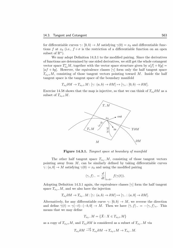
14.3. Tangent and Cotangent 563
for differentiable curves γ : [0, b)→M satisfying γ(0) = x0 and differentiable func-tions f at x0 (i.e., f σ is the restriction of a differentiable function on an opensubset of Rn).
We may adopt Definition 14.3.1 to the modified pairing. Since the derivativesof functions are determined by one sided derivatives, we still get the whole cotangentvector space T ∗x0
M , together with the vector space structure given by a[f ] + b[g] =[af + bg]. However, the equivalence classes [γ] form only the half tangent spaceTx0+M , consisting of those tangent vectors pointing toward M . Inside the halftangent space is the tangent space of the boundary manifold
Tx0∂M → Tx0+M : [γ : (a, b)→ ∂M ] 7→ [γ+ : [0, b)→ ∂M ].
Exercise 14.58 shows that the map is injective, so that we can think of Tx0∂M as asubset of Tx0+M .
[0,b)
(a, 0
]
out
in
T−M
T+M T∂M
x0
M ∂M
Figure 14.3.1. Tangnet space at boundary of manifold
The other half tangent space Tx0−M , consisting of those tangent vectorspointing away from M , can be similarly defined by taking differentiable curvesγ : (a, 0]→M satisfying γ(0) = x0 and using the modified pairing
〈γ, f〉− =d
dt
∣∣∣∣t=0−
f(γ(t)).
Adopting Definition 14.3.1 again, the equivalence classes [γ] form the half tangentspace Tx0−M , and we also have the injection
Tx0∂M → Tx0−M : [γ : (a, b)→ ∂M ] 7→ [γ− : (a, 0]→ ∂M ].
Alternatively, for any differentiable curve γ : [0, b) → M , we reverse the directionand define γ(t) = γ(−t) : (−b, 0] → M . Then we have 〈γ, f〉− = −〈γ, f〉+. Thismeans that we may define
Tx0−M = X : X ∈ Tx0+M
as a copy of Tx0+M , and Tx0∂M is considered as a subset of Tx0−M via
Tx0∂M
−id−→ Tx0∂M → Tx0+M → Tx0−M.

564 Chapter 14. Manifold
The whole tangent space Tx0M may be obtained by glueing the two halftangent spaces along the subset Tx0∂M . We also note that for functions defined onopen subsets of Rn, we have 〈γ, f1〉+ = 〈γ, f2〉+ for all γ : [0, b) → M if and onlyif 〈γ, f1〉− = 〈γ, f2〉− for all γ : (a, 0] → M . This implies that applying Definition14.3.1 to 〈γ, f〉− gives the same cotangent space T ∗x0
M as 〈γ, f〉+.
Proposition 14.3.4. The tangent and cotangent spaces Tx0M and T ∗x0
M of a dif-ferentiable manifold M at a boundary point x0 ∈ ∂M have natural vector spacestructures, and Tx0
M and T ∗x0M form a dual paring.
Proof. Similar to the proof of Proposition 14.3.2, we introduce
(σ−1)′(x0) : Tx0M → Rn,
[[0, b)
γ→M ] 7→ (σ−1 γ)′+(0),
[(a, 0]γ→M ] 7→ (σ−1 γ)′−(0);
σ′(~u0) : Rn → Tx0M, ~v 7→ [σ(~u0 + t~v)]
t ≥ 0, if ~v ∈ Rn+,t ≤ 0, if ~v ∈ Rn−.
The maps for the cotangent space are the same as before. Then we verify that themaps are well defined, inverse to each other, induce vector space structure, and givedual pairing, similar to the proofs of Propositions 14.3.2 and 14.3.3.
Exercise 14.57. Suppose U is an open subset of Rn+ and ~u0 ∈ U ∩Rn−1× 0. Prove that thefollowing is equivalent for a function g on U .
1. g has linear approximation on U at ~u0.
2. g is the restriction of a function on an open subset of Rn that is differentiable at u0.
Exercise 14.58. Prove that the map Tx0∂M → Tx0+M is well defined and injective. Thismeans that the equivalence in Tx0∂M as tested by differentiable functions on ∂M is thesame as the equivalence in Tx0+M as tested by differentiable functions on M .
Exercise 14.59. Complete the proof of Proposition 14.3.4.
Exercise 14.60. Prove that T ∗x0∂M is naturally a quotient vector space of T ∗x0M . Moreover,prove that the dual pairing between Tx0∂M and T ∗x0∂M is compatible with the dual pairingbetween Tx0M and T ∗x0M , with respect to the inclusion Tx0∂M ⊂ Tx0M and the quotientT ∗x0M → T ∗x0∂M .
14.4 Differentiable MapSince manifolds are locally identified with (open subsets of) Euclidean spaces, manyaspects of the differentiation and integration can be carried out on manifolds. Theusual modus operandi is to use charts to pull whatever happens on the manifoldto the Euclidean space and then do the calculus on the Euclidean space. If we canshow that this is independent of the choice of charts, then what we have done isreally happening on the manifold itself. We have done this for the sequence limit,the tangent and cotangent spaces, and the dual pairing between them.
14.4. Differentiable Map 565
Differentiable Map
Definition 14.4.1. A map F : M → N between differentiable manifolds is differen-tiable, if F is continuous and, for any charts σ : U →Mσ ⊂M and τ : V → Nτ ⊂ Nsatisfying F (Mσ) ⊂ Nτ , the composition τ−1 F σ is differentiable.
The property F (Mσ) ⊂ Nτ is needed for the composition τ−1 F σ to makesense. Proposition 14.2.13 says that we can always arrange to have F (Mσ) ⊂ Nτeverywhere.
If M and N are Cr-manifolds and the composition τ−1 F σ is r-th ordercontinuously differentiable, then we say F is r-th order differentiable, or a Cr-map.The Cr requirement on M and N makes sure that the definition is independent ofthe choice of Cr-compatible charts.
Exercise 14.61. Prove that the differentiability is independent of the choice of charts. Morespecifically, prove that if τ−1 F σ is differentiable for one pair of charts σ and τ , thenτ−1 F σ is differentiable on the overlapping for any other pair of charts σ and τ .
Exercise 14.62. Prove that composition of differentiable maps is differentiable.
Exercise 14.63. Prove that any chart σ : U →M is differentiable, and the inverse σ−1 : σ(U)→U is also differentiable.
Exercise 14.64. Prove that a function f : M → R is differentiable if and only if for anychart σ : U →M , the composition f σ is a differentiable function on U ⊂ Rn.
Exercise 14.65. Prove that a curve γ : (a, b) → M is differentiable if and only if for anyt ∈ (a, b) and any chart σ : U →M around γ(t0), there is δ > 0, such that γ(t− δ, t+ δ) ⊂σ(U), and σ−1 γ : (t− δ, t+ δ)→ U ⊂ Rn is differentiable.
Exercise 14.66. Prove that under the set up in Exercise 14.43, the map F is differentiableif and only if the composition τ−1
i F σi : Ui → Vi is differentiable for each i.
Exercise 14.67. For differentiable manifolds M and N , prove that the projection map M ×N →M and the inclusion map M →M × y0 ⊂M ×N are differentiable.
For a map F : Rm → Rn, the derivative F ′(~x0) : Rm → Rn is the lineartransform in the first order term in the linear approximation of F
F (~x) = F (~x0) + F ′(~x0)(~x− ~x0) + o(~x− ~x0).
To extend to maps between differentiable manifolds, we also need to linearly ap-proximate the manifolds by the tangent spaces. So the derivative of a differentiablemap F : M → N at x0 ∈M should be a linear transform F ′(x0) : Tx0M → TF (x0)N .
Definition 14.4.2. Let F : M → N be a differentiable map between differentiable

566 Chapter 14. Manifold
manifolds. The derivative (or pushforward) of F is
F∗ = F ′(x0) : Tx0M → TF (x0)N, [γ] 7→ [F γ].
The pullback of F is
F ∗ : T ∗F (x0)N → T ∗x0M, [f ] 7→ [f F ].
The derivative F ′ is also called pushforward because it goes in the same di-rection of F . Such behaviour is called covariant, and is often denoted by subscript∗. The map F ∗ on cotangent vectors is called pullback because it goes in the op-posite direction of F . Such behaviour is called contravariant, and is often denotedby superscript ∗. The pullback can also be applied to differentiable functions onmanifolds because it is also contravariant
F ∗ : C1(N)→ C1(M), f 7→ f F.
This is a linear transform and actually an algebraic homomorphism. Then thedefinition F ∗[f ] = [f F ] of pullback means
F ∗df = dF ∗f. (14.4.1)
For a tangent vector X ∈ Tx0M and a differentiable function f at F (x0) ∈ N ,
the definition of the derivative means
F∗X(f) = F ′(x0)(X)(f) =d
dt
∣∣∣∣t=0
f(F γ(t))
=d
dt
∣∣∣∣t=0
(f F )(γ(t)) = X(f F ) = X(F ∗f). (14.4.2)
The first line happens on N , and the second line happens on M . The equalityimplies that F∗ = F ′(x0) is well defined. For ω = df , the equality (14.4.2) can berephrased as
〈F∗X,ω〉 = 〈X,F ∗ω〉, X ∈ TM, ω ∈ T ∗N.This shows exactly that F∗ and F ∗ form a dual pair of linear transforms.
Example 14.4.1. A chart σ : U → M around ~x0 = σ(u0) is differentiable. Its inverseσ−1 : σ(U) → U is also differentiable. See Exercise 14.63. Then we get derivatives (orpushforwards)
σ∗ = σ′(~u0) : T~u0U → Tx0M, (σ−1)∗ = (σ−1)′(x0) : Tx0M → T~u0U,
and pullbacks
σ∗ = σ′(~u0)∗ : T ∗x0M → T ∗~u0U, (σ−1)∗ = (σ−1)′(x0)∗ : T ∗~u0
U → T ∗x0M.
Combined with the isomorphisms T~u0U∼= Rn and T ∗~u0
U ∼= (Rn)∗ in Example 14.3.1, weget
σ′(~u0) : Rn ∼= T~u0U → Tx0M, ~v 7→ [~u0 + t~v] 7→ [σ(~u0 + t~v)];
(σ−1)′(x0) : Tx0M → T~u0U∼= Rn, [γ] 7→ [σ−1 γ] 7→ (σ−1 γ)′(0);
σ′(~u0)∗ : T ∗x0M → T ∗~u0U ∼= (Rn)∗, [f ] 7→ [f σ] 7→ (f σ)′(~u0);
(σ−1)′(x0)∗ : (Rn)∗ ∼= T ∗~u0U → T ∗x0M, l 7→ [l] 7→ [l σ−1].
14.4. Differentiable Map 567
This explains the notations for the isomorphisms in Proposition 14.3.2.
Example 14.4.2. A function f : M → R is differentiable if and only if for any chart σ : U →M , the composition fσ is differentiable. See Exercise 14.64. The derivative of the functionis a linear functional on the tangent space
f∗[γ] = f ′(x0)([γ]) = [f γ] = (f γ)′(0) : Tx0M → Tf(x0)R ∼= R.
Here the second equality is the definition of the derivative f ′(x0) : Tx0M → Tf(x0)R,and the third equality is the isomorphism Tf(x0)R ∼= R in Example 14.3.1. By (14.3.2),(f γ)′(0) is simply the pairing between the tangent vector X = [γ] and the cotangentvector df = [f ]. Therefore the linear functional f∗ = f ′(x0) is exactly the differentialf ′(x0) = dx0f ∈ T ∗x0M .
Alternatively, the differentiable function induces a pullback f∗ : T ∗R→ T ∗x0M . Thestandard basis in T ∗R is the differential dt of the identity linear functional t 7→ t : R→ R(the standard basis of R∗). The pullback f∗ is determined by f∗dt = [(t 7→ t) f ] = [f ] =df . Therefore the pullback f∗ is naturally identified with its differential df ∈ T ∗x0M .
Example 14.4.3. Let γ : (a, b) → M be a differentiable curve. See Exercise 14.65. Thederivative linear transform
γ′(t0) : R = Tt0(a, b) 7→ Tγ(t0)M
is determined by its value γ′(t0)(1) ∈ Tγ(t0)M at 1 ∈ R. We abuse the notation by simplyalso use γ′(t0) to denote the tangent vector γ′(t0)(1) of the curve.
Note that 1 ∈ R corresponds to the equivalence class [t0 + t ·1] ∈ Tt0(a, b). Thereforethe tangent vector of the curve
γ′(t0) = γ′(t0)(1) = [γ(t0 + t)]at t=0 = [γ(t)]at t=t0 ∈ Tγ(t0)M
is exactly the equivalence class represented by the curve itself.
Exercise 14.68. Prove that the pullback of cotangent vectors is well defined. In other words,[f F ] depends only on the equivalence class [f ].
Exercise 14.69. Formulate and prove the chain rules for the derivative and the pullback.
Exercise 14.70. Extend the discussion in Example 14.4.2 to vector valued functions f : M →Rm.
Exercise 14.71. What is the pullback of a continuously differentiable curve γ : (a, b)→M?
Exercise 14.72. What is the derivative and the pullback of the diagonal map F (x) =(x, x) : M →M ×M?
Exercise 14.73. Describe the derivatives and the pullbacks of the projection map M×N →M and the inclusion map M →M × y0 ⊂M ×N .
Exercise 14.74. A submanifold M of RN has a natural inclusion map i : M → RN . Provethat the tangent space defined in Section 8.4 is the image of the injective derivative mapi′(~x0) : T~x0M → T~x0R
N ∼= RN .

568 Chapter 14. Manifold
Exercise 14.75. Prove that the derivative of the map F (x, y, z) = (x2−y2, xy, xz, yz) : R3 →R4 at (x, y, z) is injective as long as x 6= 0 or y 6= 0. Then prove that the derivative of therestriction F : S2 → R4 of F is always injective.
Differentiation in Charts
Let σ and τ be charts satisfying F (σ(U)) ⊂ τ(V ), and x0 = σ(~u0), F (x0) = τ(~v0).Then the map τ−1 F σ : U ⊂ Rm → V ⊂ Rn is explicit expressions of thecoordinates (v1, v2, . . . , vn) of V as functions of the coordinates (u1, u2, . . . , um)of U . The tangent spaces Tx0M and TF (x0)N have bases ∂u1 , ∂u2 , . . . , ∂um and∂v1 , ∂v2 , . . . , ∂vn, and we have
F∗∂ui = ai1∂v1 + ai2∂v2 + · · ·+ ain∂vn .
By (14.3.5), the coefficients are
aij = F∗∂ui(vj) = ∂ui(vj F ) =∂vj∂ui
.
Therefore
F∗∂u1=∂v1
∂u1∂v1 +
∂v2
∂u1∂v2 + · · ·+ ∂vn
∂u1∂vn ,
F∗∂u2=∂v1
∂u2∂v1 +
∂v2
∂u2∂v2 + · · ·+ ∂vn
∂u2∂vn ,
...
F∗∂um =∂v1
∂um∂v1 +
∂v2
∂um∂vn + · · ·+ ∂vn
∂um∂vn .
The coefficients form the Jacobian matrix of the map τ−1 F σ.
Example 14.4.4. In Example 14.2.5, we find the explicit formula for the canonical mapF (~x) = [~x] : Sn → RPn
τ−10 F σ0(~u) =
~u√1− ‖~u‖22
: U → V
in terms of two charts of Sn and RPn. Taking ~u = ~u0 + t~v, we get
τ−10 F σ0(~u) =
~u0 + t~v√1− ‖~u0 + t~v‖22
= (~u0 + t~v)[1− ‖~u0‖2 − 2(~u0 · ~v)t+ o(t)
]− 12
= (~u0 + t~v)(1− ‖~u0‖2
)− 12
[1− 2
~u0 · ~v1− ‖~u0‖2
t+ o(t)
]− 12
=~u0√
1− ‖~u0‖22+
1√1− ‖~u0‖22
[~v +
~u0 · ~v1− ‖~u0‖2
~u0
]t+ o(t).

14.4. Differentiable Map 569
Therefore the explicit formula for the derivative is
(τ−10 F σ0)′(~u0)(~v) =
1√1− ‖~u0‖22
[~v +
~u0 · ~v1− ‖~u0‖2
~u0
].
The derivative is the identity at ~u0 = ~0, and is the following at ~u0 6= ~0
(τ−10 F σ0)′(~u0)(~v) =
~v√
1− ‖~u0‖22, if ~v ⊥ ~u0,
~v
(√
1− ‖~u0‖22)3, if ~v ‖ ~u0.
Similar charts σi and τi can be found for xi > 0 and for xi 6= 0, as well as for xi < 0and for xi 6= 0. The differentiations can also be calculated.
Example 14.4.5. Let F (ξ) = 2ξ : Sn12→ Sn be the scaling map from the sphere of radius
1
2to the unit sphere. The stereographic projections in Example 14.1.3 give an atlas for
Sn12. Let ξ = (η, z), with η ∈ Rn and z ∈ R. Since the triangles Nξ~v and Sξ~u are similar
at the ratio of ‖~v‖ : ‖~u‖, we get
‖η‖‖~u‖ =
‖~v‖‖~u‖+ ‖~v‖ , z =
1
2
‖~u‖‖~u‖+ ‖~v‖ −
1
2
‖~v‖‖~u‖+ ‖~v‖ =
1
2
‖~u‖ − ‖~v‖‖~u‖+ ‖~v‖ .
Then by η parallel to ~v and ‖~u‖‖~v‖ = 1, we get
η =‖~u‖‖~v‖‖~u‖+ ‖~v‖
~v
‖~v‖ =~v
1 + ‖~v‖2 , z =1
2
1− ‖~v‖2
1 + ‖~v‖2 , 2ξ =(2~v, 1− ‖~v‖2)
1 + ‖~v‖2 .
On the other hand, the upper half unit sphere has a chart
σ0(~w) =(~w,√
1− ‖~w‖2)
: ~w ∈ Rn : ‖~w‖ < 1 → Sn.
Then we have
σ−10 F σS(~v) =
2~v
1 + ‖~v‖2 : ~v ∈ Rn : ‖~v‖ < 1 → ~w ∈ Rn : ‖~w‖ < 1.
Taking ~v = ~v0 + t~a, we get
σ−10 F σS(~v) =
2(~v0 + t~a)
1 + ‖~v0 + t~a‖2
=2(~v0 + t~a)
1 + ‖~v0‖2 + 2(~v0 · ~a)t+ o(t)
=2(~v0 + t~a)
1 + ‖~v0‖2
[1− 2
~v0 · ~a1 + ‖~v0‖2
t+ o(t)
]=
2~v0
1 + ‖~v0‖2+
2
1 + ‖~v0‖2
[~a− 2
~v0 · ~a1 + ‖~v0‖2
~v0
]t+ o(t).
The derivative is
(σ−10 F σS)′(~v0)(~a) =
2
1 + ‖~v0‖2~a, if ~a ⊥ ~v0,
2(1− ‖~v0‖2)
(1 + ‖~v0‖2)2~a, if ~a ‖ ~v0.

570 Chapter 14. Manifold
Exercise 14.76. Given charts of M and N , the cotangent spaces T ∗M and T ∗N have basesdui and dvj . Find the explicit formula for the pullback in terms of the bases.
Exercise 14.77. Show that the obvious map M → S1 : (z, v) 7→ z from the open Mobiusband in Example 14.1.4 to the circle is differentiable. Moreover, construct the obviousinclusion map S1 →M and show that it is differentiable.
Exercise 14.78. For the Mobius band in Example 14.1.9, construct the obvious map M →S1 and two maps S1 → M , one being similar to the one in Exercise 14.77, and the otherbeing the boundary of the Mobius band. Show that all three maps are differentiable.
Exercise 14.79. Show that the canonical map S2n+1 → CPn is differentiable and find thederivative in terms of suitable charts.
Exercise 14.80. By thinking of real numbers as complex numbers, we have the map RPn →CPn. Show that the map is injective and differentiable.
Diffeomorphism
Definition 14.4.3. A diffeomorphism between differentiable manifolds is an invert-ible map F : M → N , such that both F and F−1 are differentiable.
Given the diffeomorphism F , whatever differentiation or integration on Mcan be translated by F to differentiation or integration on N , and vice versa. Inparticular, calculus on M is equivalent to calculus on N .
Example 14.4.6. For a a continuously differentiable map F : U ⊂ Rn → RN−n, its graph
ΓF = (~x, F (~x)) : ~x ∈ U ⊂ RN
is a manifold. The maps
U → ΓF : ~x 7→ (~x, F (~x)), ΓF → U : (~x, ~y) 7→ ~x
are inverse to each other and are continuously differentiable. Therefore ΓF and U arediffeomorphic.
In general, Exercise 14.63 says that if σ : U → M is a chart covering the wholemanifold M : σ(U) = M , then σ is a diffeomorphism between U and M .
Example 14.4.7. The sphere of half radius in Example 14.1.3 and the complex projectivespace CP 1 in Example 14.1.6 are covered by two charts, with transition maps
ϕNS(u, v) =(u, v)
u2 + v2, ϕ10(u, v) =
(u,−v)
u2 + v2: R2 − (0, 0)→ R2 − (0, 0).
The transitions become the same if we modify σN (u, v) to σN (u,−v). This suggests thatS2 and CP 1 are diffeomorphic. See Exercise 14.8.
Specifically, denote vectors (u, v) ∈ R2 by complex numbers w = u + iv ∈ C. Thenthe modification (u, v) 7→ (u,−v) means taking the complex conjugation w of w. According

14.4. Differentiable Map 571
to the calculation in Example 14.4.5, the sphere S2 ⊂ C×R of unit radius is given by thefollowing modified stereographic projection charts
σS(w) = 2σS(w) =(2w, 1− |w|2)
1 + |w|2 , σN (w) = 2σN (w) =(2w, |w|2 − 1)
|w|2 + 1.
Then the transition ϕNS = σ−1N σS(w) =
1
wis equal to the transition ϕ10(w) =
1
w, and
the diffeomorphism F : CP 1 → S2 should be given by F (σ0(w)) = σS(w) and F (σ1(w)) =σN (w). This means
F ([1, w]) =(2w, 1− |w|2)
1 + |w|2 , F ([w, 1]) =(2w, |w|2 − 1)
|w|2 + 1,
or
F ([w0, w1]) =(2w0w1, |w0|2 − |w1|2)
|w0|2 + |w1|2: CP 1 → S2 ⊂ C× R.
By (σ−1S F σ0)(w) = w and (σ−1
N F σ1)(w) = w, both F and F−1 are differentiable.Roughly speaking, the identification of S2 and CP 1 is given by
S2 ∼= C ∪∞ → CP 1 : w 7→ [w, 1], ∞ 7→ [1, 0],
and
CP 1 → C ∪∞ ∼= S2 : [w0, w1] 7→ w1
w0, [0, w1] 7→ ∞.
Here ∞ is the south pole, and C is regarded as a subset of S2 through the stereographicprojection σS . The formulae we derived above make the idea rigorous.
Exercise 14.81. Show that the circle S1 and the real projective space RP 1 are diffeomorphic.See Exercise 14.7.
Local Diffeomorphism
Definition 14.4.4. A differentiable map F : M → N is a local diffeomorphism if forany F (x) = y, there is an open neighbourhood B of x, such that F (B) is an openneighbourhood of y, and F : B → F (B) is a diffeomorphism.
The Inverse Function Theorem (Theorem 8.3.1) says that the invertibility ofa map between open subsets of Rn can be locally detected by the invertibility of itslinear approximation. By using the charts to translate maps between manifolds tothis special case, we get the manifold version of the Inverse Function Theorem.
Theorem 14.4.5 (Inverse Function Theorem). A continuously differentiable map be-tween differentiable manifolds is a local diffeomorphism if and only if its derivativeis invertible everywhere.
Example 14.4.8. The map F (θ) = (cos θ, sin θ) : R→ S1 is not a diffeomorphism becauseit sends infinitely many θ to the same point on the circle. However, if 0 < δ < π, then forany θ, the map F : (θ−δ, θ+δ) is a diffeomorphism. Therefore F is a local diffeomorphism.

572 Chapter 14. Manifold
Example 14.4.9. In Example 14.2.5, we find the explicit formula for the canonical mapF (~x) = [~x] : Sn → RPn in terms of one pair of charts. In Example 14.4.4, we furthercalculated the derivative of the explicit formula and find that the derivative is invertible.Therefore the map is a local diffeomorphism at least on the related chart. Similar compu-tation shows that the map is a local diffeomorphism on all the other charts. Therefore Fis a local homeomorphism.
In fact, F is a two-to-one map because two unit length vectors ~x and ~y span thesame 1-dimensional subspace if and only if ~x = ±~y. If we restrict to the chart σ0, which isthe half sphere with x0 > 0, then the explicit formula for τ−1
0 F σ0 in Example 14.4.4is a full diffeomorphism between the charts σ0 and τ0. This explicitly shows that F is alocal diffeomorphism on σ0. The same happens to the other charts.
Exercise 14.82. Prove that the map F : S1 → S1 that sends angle θ to 5θ is a local diffeo-morphism. What about sending θ to π − 3θ?
Exercise 14.83. Construct a local diffeomorphism from the open Mobius band in Example14.1.4 to itself, such that z(θ) goes to z(3θ). Moreover, construct a local diffeomorphismfrom the cylinder S1 × R to the open Mobius band, such that z(θ) goes to z(2θ).
Exercise 14.84. Prove that an invertible local diffeomorphism is a diffeomorphism.
Exercise 14.85. The map F : S2 → R4 in Exercise 14.75 satisfies F (−~x) = F (~x) and there-fore induces a map G[~x] = F (~x) : RP 2 → R4. Prove that the derivative of G is alwaysinjective.
14.5 OrientationA differentiable manifold has a tangent vector space at every point. An orientationof the manifold is a compatible choice of one orientation for each tangent space.The compatibility comes from the following isomorphism between tangent spacesat nearby points. For any x0, let σ : U → M be a chart around x0 = σ(~u0). Thenfor each x = σ(~u), we have isomorphism
σ′(~u) σ′(~u0)−1 : Tx0M
σ′(~u0)←−−−−∼= Rn σ′(~u)−−−→∼= TxM. (14.5.1)
The compatibility means that the isomorphism translates the orientation of Tx0M
to the orientation of TxM .
Definition 14.5.1. An orientation of a differentiable manifold M is a choice of anorientation ox of the tangent space TxM for each x ∈ M satisfying the followingcompatibility condition: For any x0, there is a chart σ : U → M around x0, suchthat for every x = σ(~u), the isomorphism (14.5.1) translates the orientation ox0
tothe orientation ox. A differentiable manifold is orientable if it has an orientation.Otherwise it is non-orientable.
The compatibility condition should be independent of charts. Suppose τ : V →M is another chart containing x0 = τ(~v0). By shrinking σ(U) and τ(V ) (i.e.,

14.5. Orientation 573
restricting σ and τ to smaller open subsets) to the connected component of σ(U)∩τ(V ) containing x0, we may assume that σ(U) = τ(V ), and U and V are connected.Now we compare the isomorphisms (14.5.1) for the two charts
TxMτ ′(~v)←−−−∼= Rn τ ′(~v0)−−−−→∼= Tx0
Mσ′(~u0)←−−−−∼= Rn σ′(~u)−−−→∼= TxM.
Let ϕ = σ−1 τ be the transition between the two charts. By Exercise 7.57, we get
det(σ′(~u) σ′(~u0)−1 τ ′(~v0) τ ′(~v)−1)
= det(σ′(~u0)−1 τ ′(~v0) τ ′(~v)−1 σ′(~u))
= det(ϕ′(~u0) ϕ′(~u)−1
) = (detϕ′(~u0))(detϕ′(~u))−1.
Since this is a continuous non-vanishing function on connected U , and takes value1 at ~u = ~u0, by Proposition 6.2.4, it is positive throughout U . This implies that ifσ translates ox0
to ox, then τ also translates ox0to ox. Therefore the translation of
orientation at x0 to nearby x is independent of the charts, as long as x lies in theconnected component of the overlapping containing x0.
Exercise 14.86. Suppose three points x, y, z are contained in a chart σ, and ox, oy, oz areorientations at the three points. Prove that if σ translates ox to oy and oy to oz, then σtranslates ox to oz.
Exercise 14.87. Prove that if a chart translates ox to oy, then it translates −ox to −oy,and translates oy to ox.
Exercise 14.88. Suppose M is an oriented manifold. Prove that the choices −ox also givean orientation of M . We usually denote the manifold with −ox orientation by −M .
Exercise 14.89. Prove that any open subset of an orientable manifold is orientable.
Exercise 14.90. Suppose M and N are oriented. Construct the product orientation onM × N by using Exercises 7.78 and 14.54, and then prove that M × N is also oriented.Conversely, if M ×N is orientable, must M and N be orientable?
Exercise 14.91. Prove that if M and N are oriented manifolds, then the product orientationsatisfies M ×N = (−1)mnN ×M , m = dimM , n = dimN .
Translation of Orientation Along Curve
Suppose ox0is an orientation at one point x0 ∈ M . Suppose γ : [0, 1] → M is
a continuous path starting at γ(0) = x0. For each t ∈ [0, 1], there is an interval(t − δt, t + δt) and a chart σt : Ut → M , such that γ(t − δt, t + δt) ⊂ σ(Ut). Here,γ(t) = γ(0) for t < 0 and γ(t) = γ(1) for t > 1. The bounded closed interval [0, 1] iscovered by open intervals (t−δt, t+δt), t ∈ [0, 1]. By Heine-Borel Theorem (Theorem1.5.6) and changing notations, we get [0, 1] ⊂ (a0, b0)∪ (a1, b1)∪ · · · ∪ (ak, bk), suchthat each segment γ(ai, bi) is contained in a chart σi : Ui →M . Moreover, we may

574 Chapter 14. Manifold
assume the intervals are arranged in “ascending order”, in the sense that there is apartition 1 = t0 < t1 < · · · < tk = b, such that ti ∈ (ai−1, bi−1) ∩ (ai, bi).
x0 x1
x2
xkTx0M
Tx1M
TxkM
σ0σ1
σk
Figure 14.5.1. Translation of orientation along a curve
We may use σ0 to translate the orientation ox0at x0 = γ(t0) to an orientation
ox1at x1 = γ(t1). Then may use σ1 to translate the orientation ox1
to an orientationox2 at x2 = γ(t2). Keep going, we get an orientation oxk at xk = γ(1) at the end.
To see that the translation from ox0 to oxk is unique, we compare two partitionsand the corresponding sequences of charts. By using the common refinement, wemay assume that one partition is a refinement of another. Then the problem isreduced to comparing the translation of an orientation at xi−1 to an orientationat xi by using one chart σi, and the translation by following a sequence xi−1 =y0, y1, . . . , yl = xi and using a sequence of charts τ0, τ1, . . . , τl from the refinement.Since the curve segment between yj−1 and yj is connected and is therefore containedin the connected component of the overlapping between σi and τj , the translationof an orientation from yj−1 to yj by using τj is the same as the translation by usingσi. Therefore we may assume that all τj are equal to σi. Then by Exercise 14.86,it is easy to see that the two translations are the same.
Exercise 14.92. Extend Exercises 14.86 and 14.87 to the translation along a curve.
Suppose M is a connected manifold, and an orientation ox0is fixed. For any
x ∈M , there is a curve γ connecting x0 to x, and we may translate ox0 along γ to anorientation ox at x. Like the integral of 1-form along a curve, the problem is whetherthe translation depends on the choice of γ. If the translation does not depend onthe choice, then we get a well defined orientation ox at each point x ∈ M . Theuse of translation in constructing the orientations ox implies that the compatibilitycondition is satisfied. Therefore the orientation ox0
at one point determines anorientation of M .
In general, a manifold is orientable if and only if each connected component isorientable. Moreover, an orientation is determined by the choice of an orientationat one point of each connected component.
It is easy to see that the translation along two curves give different orientationsat the end if and only if the translation of an orientation o along a loop (a curve

14.5. Orientation 575
starting and ending at the same point) gives the negative orientation −o. This isequivalent to the non-orientability of the manifold, and is also equivalent to thatthe manifold contains (Mobius band)× Rn−1 as an open subset.
Orientation Compatible Atlas
Suppose M is an oriented manifold. A chart σ : U → M is orientation compatibleif the isomorphism σ′(~u) : Rn → TxM always translates the standard orientation ofRn to the orientation ox of TxM . In other words, ox is given by the standard basis∂u1
, ∂u2, . . . , ∂un of TxM .
An atlas is orientation compatible if all its charts are orientation compatible.Suppose σ and τ are two charts in such an atlas, and x = σ(~u) = τ(~v) is a point inthe overlapping. Then both isomorphisms
σ′(~u) : Rn ∼= TxM, τ ′(~v) : Rn ∼= TxM,
translate the standard orientation of Rn to the same orientation ox of TxM . Thisimplies that the composition τ ′(~v)−1 σ′(~u) = ϕ′(~u) preserves the orientation ofTxM . This means that the derivative of the transition map has positive determi-nant. The property is used for defining the integral of 2-forms in (13.2.6).
Proposition 14.5.2. A differentiable manifold is orientable if and only if there isan atlas, such that the determinants of the derivatives of the transition maps areall positive.
Proof. Suppose M has an orientation given by ox for every x ∈ M . Then for anyx0, there is a chart σ : U → Rn containing x0 = σ(~u0), such that the isomorphism(14.5.1) translates ox0
to ox for any x = σ(~u), ~u ∈ U . If σ′(~u0) translates thestandard orientation o of Rn to ox0 , then this implies that σ′(~u) translates o to ox.If σ′(~u0) translates the negative −o of sthe tandard orientation of Rn to ox0 , thenfor the modified chart
τ = σ J−1 : J(U)→M, J(u1, u2, . . . , un) = (−u1, u2, . . . , un),
τ ′(J(~u0)) translates the standard orientation o to ox0. The same argument as
before shows that τ ′(J(~u)) translates o to ox. We conclude that either σ or σ J is an orientation compatible chart. This proves that every point is containedin an orientation compatible chart. Combining these charts together, we get anorientation compatible atlas. As argued before the proposition, the derivatives ofthe transition maps in this atlas have positive determinants.
Conversely, suppose there is an atlas σi, such that the derivatives of allthe transition maps have positive determinants. For any x ∈ M , take a chartσi containing x and define the orientation ox to be the translation of o via theisomorphism σ′i(~u) : Rn ∼= TxM , x = σi(~u). Since detϕ′ji > 0, the transitionmaps preserve orientations, so that ox is independent of the choice of chart. Theconstruction of ox also implies that the compatibility condition in Definition 14.5.1is satisfied. Therefore we get an orientation for M .

576 Chapter 14. Manifold
Example 14.5.1. The tangent space of S1 at a point is 1-dimensional, and its orientationis given by one basis vector. Therefore an orientation of S1 is given by a nonzero tangentfield. An example is to choose the tangent vector at ~x ∈ S1 to be the counterclockwiserotation R(~x) of ~x by 90 degrees.
To verify the compatibility condition, we cover the unit circle by two charts
σ0(θ) = (cos θ, sin θ) : (0, 2π)→ S1, σ1(θ) = (cos θ, sin θ) : (−π, π)→ S1.
The derivative isomorphism of the first chart is
Rσ′0(θ)−−−→∼=
T~xS1 : 1 7→ (− sin θ, cos θ) = R(~x), ~x = σ0(θ).
Therefore the derivative translates the standard orientation (given by the basis 1 of R)to the orientation of T~xS
1 (given by the basis R(~x) of T~xS1). The same happens to the
chart σ1. This verifies the compatibility, and also shows that the charts are orientationcompatible.
We may also choose charts
σ0(θ) = (cos θ, sin θ) : (0, 2π)→ S1, σ1(θ) = (sin θ, cos θ) : (0, 2π)→ S1.
The transition map has two parts
ϕ10(θ) =
π
2− θ :
(0,π
2
)→(
0,π
2
),
5π
2− θ :
(π2, 2π)→(π
2, 2π),
and ϕ′10 = −1 < 0 on both parts. However, the negative sign does not mean the circle isnot orientable. It only means that we need to compose the σ1 with J(θ) = −θ to get newσ1
σ1(θ) = (sin(−θ), cos(−θ)) = (− sin θ, cos θ) : (−2π, 0)→ S1.
Then the derivative of the transition between the two charts is +1.Similar situation happened in Example 13.2.7, where we carefully choose the order
of variables in the parameterizations, to make sure that all the pieces give the same normalvector, and the derivatives of the transition maps have positive determinants.
Example 14.5.2. Consider the open Mobius band in Example 14.1.4. The transition maphas two parts, with det(ϕ+
10)′ = 1 and det(ϕ−10)′ = −1. Unlike Example 14.5.1, no ad-justment of the orientation for the charts can make the determinant positive everywhere.Specifically, since the charts are connected, if we change the orientation for σ1, then wewill only get det(ϕ+
10)′ negative and det(ϕ−10)′ positive. The problem is that any adjust-ment will change both signs simultaneously, and therefore cannot make both positive. TheMobius band is not orientable.
Example 14.5.3. The real projective space RP 2 in Example 14.1.5 is covered by threeconnected charts σi, i = 0, 1, 2. The transition maps are
ϕ10(u, v) =
(1
u,v
u
), ϕ20(u, v) =
(1
v,u
v
), ϕ21(u, v) =
(u
v,
1
v
).
We have
detϕ′10 = − 1
u3, detϕ′20 =
1
v3, detϕ′21 = − 1
v3.
In fact, each transition map is broken into two parts, and detϕ′ji have different signs onthe two parts. Similar to Example 14.5.2, the real projective space RP 2 is not orientable.

14.5. Orientation 577
Exercise 14.93. Show that the sphere Sn is orientable.
Exercise 14.94. Show that the real projective space RPn in Example 14.1.5 is orientable ifand only if n is odd.
Exercise 14.95. Show that the complex projective space CPn in Example 14.1.6 is alwaysorientable.
Exercise 14.96. Is the Klein bottle in Exercise 14.11 orientable?
Exercise 14.97. Prove that the special linear group SL(2) in Exercise 8.58 is orientableby finding an atlas so that the determinants of the derivatives of the transition maps arepositive.
Exercise 14.98. Show that the mapping torus in Exercise 14.12 is orientable if and only ifdetL > 0.
Orientation of Manifold with Boundary
Definition 14.5.1 of orientation of manifold can be directly applied to manifold withboundary. All the discussions, including the local translation of orientation, thetranslation of orientation along curves, most of Proposition 14.5.2, and the remarkafter the proposition, are still valid. The only problem is that, at boundary points,the charts in Proposition 14.5.2 cannot be restricted to open subsets of the upperhalf space Rn+. For example, the atlas given in Example 14.1.7 for M = [0, 1]satisfies detϕ′21 = −1 < 0, while the interval should be orientable. However, if weinsist that U1 and U2 must be of the form [0, a), then it will necessarily follow thatϕ21 is a decreasing function and therefore has negative determinant.
The technical reason for the problem is that, in proving Proposition 14.5.2,we need to sometimes reverse the orientation of open subsets of Rn by composingwith J . Since J takes open subsets of Rn+ to open subsets of Rn+ only if n > 1,our problem occurs only for 1-dimensional manifold with boundary. So we have thefollowing modified version of Proposition 14.5.2.
Proposition 14.5.3. A manifold with boundary is orientable if and only if there isan atlas, in which the domain of each chart is an open subset of either Rn or Rn+,such that the determinants of the derivatives of the transition maps are all positive.In case the manifold is 1-dimensional, we may also need to use open subsets ofR− = (−∞, 0] for the charts.
In Green’s Theorem, Stokes’ Theorem and Gauss’ Theorem in Sections 13.4,13.5 and 13.6, the orientation of the boundary is defined by using the outwardnormal vector. In general, at a boundary point x0 of M , we may define an outwardvector to be any vector (see Figure 14.3.1)
~nout = [γ : (a, 0]→M, γ(0) = x0] 6∈ Tx0∂M.

578 Chapter 14. Manifold
Note that the manifold M may not carry an inner product, so that we cannot talkabout outward normal vector in general. Consequently, the outward vector is notnecessarily unique. Still, we may define the orientation of the boundary using theearlier idea.
Definition 14.5.4. An orientation of a manifold M with boundary induces an ori-entation on ∂M , by requiring that an ordered basis X1, X2, . . . , Xn−1 of Tx∂Mgives the induced orientation if the ordered basis ~nout, X1, X2, . . . , Xn−1 of TxMgives the orientation of M .
There are two things we need to do to justify the definition. The first isthe choices of the outward vector and the ordered basis X1, X2, . . . , Xn−1. ByProposition 14.3.4 and the subsequent discussion, for a chart σ : U ⊂ Rn+ → Maround x0 ∈ ∂M , we have an invertible map
(σ−1)′(x0) : (Tx0M ;Tx0+M,Tx0−M,Tx0
∂M)→ (Rn;Rn+,Rn−,Rn−1 × 0). (14.5.2)
The outward vector simply means that ~nout ∈ Tx0−M − Tx0∂M . This is equivalent
to that(σ−1)′(x0)(~nout) ∈ Rn− − Rn−1 × 0
has negative last coordinate (~nout)n < 0. Since any two vectors ~w1, ~w2 ∈ Rn− −Rn−1 × 0 are related by
~w1 = λ~w2 + ~v, λ > 0, ~v ∈ Rn−1 × 0,
we see that any two outward vectors ~n1, ~n2 are related by
~n1 = λ~n2 +X, λ > 0, X ∈ Tx0∂M.
Then two choices ~n1, X1, X2, . . . , Xn−1 and ~n2, Y1, Y2, . . . , Yn−1 are related bythe matrix
λ ∗ ∗ · · · ∗0 a11 a12 · · · a1(n−1)
0 a21 a22 · · · a2(n−1)
......
......
0 a(n−1)1 a(n−1)2 · · · a(n−1)(n−1)
=
(λ ∗0 A
).
Here A is the matrix between X1, X2, . . . , Xn−1 and Y1, Y2, . . . , Yn−1. By
det
(λ ∗0 A
)= λ detA,
and λ > 0, we see that ~n1, X1, X2, . . . , Xn−1 and ~n2, Y1, Y2, . . . , Yn−1 give thesame orientation if and only if X1, X2, . . . , Xn−1 and Y1, Y2, . . . , Yn−1 give thesame orientation.
The second is to verify that the induced orientation on the boundary satisfiesthe compatibility condition in Definition 14.5.1. It is sufficient to show that σ′(~u)

14.5. Orientation 579
σ′(~u0)−1 takes an outward vector at x0 to an outward vector at x. Since withinone chart, we have the correspondence (14.5.2) of the pieces of the tangent spaceat every point in the chart, we have
Tx0−M − Tx0∂M = σ′(~u0)(Rn− − Rn−1 × 0),
Tx−M − Tx∂M = σ′(~u)(Rn− − Rn−1 × 0).
Therefore the isomorphism σ′(~u) σ′(~u0)−1 preserves the outward vector.Now we find orientation compatible charts for the boundary. Suppose σ : U ⊂
Rn+ →M is an orientation compatible chart around x0 ∈ ∂M . Then the restriction
τ = σ|Rn−1×0 : V = U ∩ Rn−1 × 0→ ∂M
is a chart of the boundary. Let X1, X2, . . . , Xn−1 be an ordered basis of Tx0∂M .
Then (σ−1)′(x0)(Xi) = ((τ−1)′(x0)(Xi), 0) ∈ Rn−1×0, and the requirement in Def-inition 14.5.4 is that (σ−1)′(x0) translates ~nout, X1, X2, . . . , Xn−1 to a positivelyoriented basis in Rn. This means that
det
(∗ (τ−1)′(X1) (τ−1)′(X2) · · · (τ−1)′(Xn−1)
(~nout)n 0 0 · · · 0
)> 0.
Since (~nout)n < 0, we get
(−1)n det((τ−1)′(X1) (τ−1)′(X2) · · · (τ−1)′(Xn−1)) > 0.
This implies that the chart τ is (−1)n-compatibly oriented. In other words, if σi isan orientation compatible atlas of M , then for even n, σi|Rn−1×0 is an orientationcompatible atlas of ∂M , and for odd n, σi|Rn−1×0 J is an orientation compatibleatlas of ∂M .
Example 14.5.4. Consider the modified atlas for M = [0, 1]
σ1(t) = t : U1 = [0, 1)→M1 = [0, 1) ⊂M,
σ2(t) = 1 + t : U2 = (−1, 0]→M2 = (0, 1] ⊂M,
that gives the orientation of M . The orientation on the 0-dimensional manifold ∂M =0, 1 simply assigns ± to the points. At 0 ∈ ∂M , we note that nout = −1 for U1, which isopposite to the orientation of [0, 1]. Therefore we correct this by assigning − to the point0. At 1 ∈ ∂M , we note that nout = 1 for U2, which is the same as the orientation of [0, 1].Therefore we keep this by assigning + to the point 1. The boundary ∂M = 0, 1 has thecompatible orientation that assigns − to 0 and + to 1.
Example 14.5.5. Let f be a continuously differentiable function on an open subset U ⊂Rn−1. Then the part of Rn over the graph of f
M = (~u, z) : z ≥ f(~u) ⊂ Rn
is a manifold with boundary, and the boundary ∂M is the graph of f . The standardorientation of Rn restricts to an orientation on M .

580 Chapter 14. Manifold
We have a natural diffeomorphism
σ(~u, t) = (~u, t+ f(~u)) : U × [0,+∞)→M,
that can be regarded as a chart covering the whole M . Since the derivative
σ′(~u0, t0)(~v, s) = (~v, s+ f ′(~u0)(~v)) : T(~u0,t0)(U × [0,+∞)) ∼= Rn → T~x0M∼= Rn
has determinant 1, the chart is compatible with the orientation of M . The restriction ofthe chart to the boundary
τ(~u) = (~u, f(~u)) : U → ∂M
is then (−1)n-compatible with the induced orientation on the graph of f . This accountsfor the sign (−1)n in (13.6.2) for the integration along the bottom piece.
For the orientation used in the integration along the top piece used in (13.6.1), weneed to consider the part of Rn below the graph of f
M = (~u, z) : z ≤ f(~u) ⊂ Rn.
The chart should be changed to
σ(~u, t) = (~u,−t+ f(~u)) : U × [0,+∞)→M,
and its derivative has determinant −1. Therefore restriction of the chart to the boundary
τ(~u) = (~u, f(~u)) : U → ∂M
is (−1)n−1-compatible with the induced orientation on the graph of f . This matches thesign (−1)n−1 in (13.6.1).
Exercise 14.99. In Example 14.5.5, the last coordinate is a function of the first n − 1coordinates. If the last coordinate is changed to the i-th coordinate, how is the restrictionof σ to Rn−1 × 0 compatible with the induced orientation on ∂M?
Exercise 14.100. Suppose σ : U →M is an orientation compatible chart around x0 ∈ ∂M ,where U is an open subset of the lower half space
Rn− = (x1, x2, . . . , xn−1, xn) : xn ≤ 0.
How is the restriction of σ to Rn−1 × 0 compatible with the induced orientation on ∂M?Then use such a chart to explain the sign (−1)n−1 in (13.6.1).
Exercise 14.101. The sphere Sn is the boundary of the unit ball Bn+1, which inherits thestandard orientation of Rn+1. Describe the induced orientation on the sphere.
Exercise 14.102. Suppose M and N are orientable manifolds with boundary. Prove that∂(M ×N) = ∂M ×N ∪ (−1)mM × ∂N , m = dimM .

Chapter 15
Field on Manifold
581
582 Chapter 15. Field on Manifold
15.1 Tangent FieldIn this chapter, we always assume that manifolds, functions, maps, and whateverquantities on manifolds are continuously differentiable of sufficiently high order.
A tangent field on a manifold M assigns a tangent vector X(x) ∈ TxM to eachpoint x ∈M . For a function f on M , X(f) is again function on M , with the valueat x obtained by applying X(x) to the function f
X(f)(x) = X(x)(f).
Flow
A flow is a time dependent movement. Suppose the point x ∈ M is at its originallocation at time t = 0 and moves to ξ(x, t) at time t. Then the flow is described bya map
ξ(x, t) : M × [0,+∞)→M, ξ(x, 0) = x.
The condition ξ(x, 0) = x means the initial position of the point. The range [0,+∞)for the time t may be too optimistic, because flows often cannot last forever. Onthe other hand, it is often convenient to allow negative time. For example, if wereset time t0 to be the initial time, then the flow is really defined for t ≥ −t0. Inthe subsequent discussion, we will assume that t ∈ (−δ, δ), and δ may depend on x.
For fixed t, the map ξt : M →M defined by ξt(x) = ξ(x, t) can be consideredas the movement from the original positions at time t. For fixed x, the curveξx : (−δ, δ) → M defined by ξx(t) = ξ(x, t) can be considered as the track of themovement of a point x. Either viewpoint is useful for understanding flows.
Example 15.1.1. The rightward movement of the plane at constant speed v is given by
ξ((x, y), t) = (x+ vt, y) : R2 × [0,+∞)→ R2.
The movement ξt at time t shifts the whole plane rightward by distance vt. The trackξ(x,y) is the horizontal line of height y.
If we restrict the flow to the unit disk U = (x, y) : x2 + y2 < 1, then ξ((x, y), t)is defined only when it lies inside U . This means that, for fixed (x, y) ∈ U , ξ((x, y), t) is
defined only for t ∈(
1v
(−√
1− y2 + x), 1v
(√
1− y2 + x))
.
Example 15.1.2. The rotation of the plane around the origin at constant angular speed vis given by
ξ((x, y), t) = (x cos vt− y sin vt, x sin vt+ y cos vt) : R2 × [0,+∞)→ R2.
The movement ξt at time t rotates the whole plane by angle vt. The track ξ(x,y) is a circleentered at the origin.
Our usual perception of the flow is the velocity∂ξ
∂t. Since the velocity is
measured at the location ξ(x, t) of x at time t, not the original location x at t = 0,

15.1. Tangent Field 583
the corresponding velocity tangent field X satisfies
X(ξ(x, t), t) =∂ξ
∂t(x, t).
If the map ξt is invertible for every t, then the velocity tangent field at time t is
Xt(x) = X(x, t) =∂ξ
∂t((ξt)
−1(x), t).
Conversely, suppose Xt(x) = X(x, t) is a (perhaps time dependent) tangentfield. Then we may recover the flow ξ(x, t) by solving
∂ξ
∂t(x, t) = X(ξ(x, t), t), ξ(x, 0) = x. (15.1.1)
For each fixed x, this is an initial value problem for an ordinary differential equationin t. The solution is the track ξx(t) of the movement of the point x in the flow.By the theory of ordinary differential equation, if the tangent field satisfies theLipschitz condition (a consequence of continuous differentiability, for example), thenthe equation has unique solution for t ∈ (−δ, δ) for some small δ that may dependon x.
Definition 15.1.1. Suppose X(x, t) is a (perhaps time dependent) tangent field ona manifold M . The flow induced by the tangent field is a map ξ(x, t) ∈M definedfor x ∈ M and small t, such that (15.1.1) holds. If ξ is defined for all t ∈ R, thenthe flow is complete.
Example 15.1.3. The rotation of the plane around the origin in Example 15.1.2 has
∂ξ
∂t((x, y), t) = (−vx sin vt− vy cos vt, vx cos vt− vy sin vt).
Since this is the tangent field X at ξ((x, y), t), or
∂ξ
∂t((x, y), t) = X(x cos vt− y sin vt, x sin vt+ y cos vt),
we getX(x, y) = (−vy, vx).
Conversely, given the tangent field X(x, y) = (−vy, vx), the corresponding flowξ((x, y), t) = (f((x, y), t), g((x, y), t)) can be found by solving the initial value problem
∂f
∂t= −vg, ∂g
∂t= vf, f = x and g = y at t = 0.
Eliminating g, we get∂2f
∂t2+ v2f = 0.
The solution is f = A cos vt + B sin vt. Substituting into the original equation, we getg = A sin vt − B cos vt. Then the initial values of f and g imply A = x,B = −y, so thatf = x cos vt− y sin vt and g = x sin vt+ y cos vt.
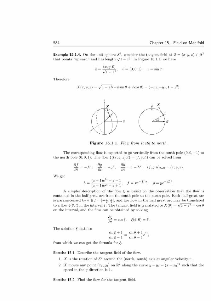
584 Chapter 15. Field on Manifold
Example 15.1.4. On the unit sphere S2, consider the tangent field at ~x = (x, y, z) ∈ S2
that points “upward” and has length√
1− z2. In Figure 15.1.1, we have
~u =(x, y, 0)√
1− z2, ~v = (0, 0, 1), z = sin θ.
Therefore
X(x, y, z) =√
1− z2(−~u sin θ + ~v cos θ) = (−xz,−yz, 1− z2).
z
y
x
~x
X
~x
X
~u
~v
θ
Figure 15.1.1. Flow from south to north.
The corresponding flow is expected to go vertically from the south pole (0, 0,−1) tothe north pole (0, 0, 1). The flow ξ((x, y, z), t) = (f, g, h) can be solved from
∂f
∂t= −fh, ∂g
∂t= −gh, ∂h
∂t= 1− h2, (f, g, h)t=0 = (x, y, z).
We get
h =(z + 1)e2t + z − 1
(z + 1)e2t − z + 1, f = xe−
∫ t0 h, g = ye−
∫ t0 h.
A simpler description of the flow ξ is based on the observation that the flow iscontained in the half great arc from the south pole to the north pole. Each half great arcis parameterised by θ ∈ I = [−π
2, π
2], and the flow in the half great arc may be translated
to a flow ξ(θ, t) in the interval I. The tangent field is translated to X(θ) =√
1− z2 = cos θon the interval, and the flow can be obtained by solving
∂ξ
∂t= cos ξ, ξ(θ, 0) = θ.
The solution ξ satisfiessin ξ + 1
sin ξ − 1=
sin θ + 1
sin θ − 1e2t,
from which we can get the formula for ξ.
Exercise 15.1. Describe the tangent field of the flow.
1. X is the rotation of S2 around the (north, south) axis at angular velocity v.
2. X moves any point (x0, y0) on R2 along the curve y − y0 = (x− x0)2 such that thespeed in the y-direction is 1.
Exercise 15.2. Find the flow for the tangent field.

15.1. Tangent Field 585
1. X = ~a is a constant vector filed on Rn.
2. X = ~a+ t~b on Rn.
3. X = (x,−y) on R2.
Exercise 15.3. Let F : M → N be a map. We say that (time independent) tangent fieldsX on M and Y on N are F -related if YF (x) = F∗Xx for all x ∈ M . Prove that the flowsξt and ηt of X and Y are also related by ηt(F (x)) = F (ξt(x)). In particular, this meansthat diffeomorphisms preserve flows of corresponding tangent fields.
Flow Diffeomorphism
A flow moves a point x from its location x1 = ξ(x, t1) at time t1 to its locationx2 = ξ(x, t2) at time t2. This suggests a map
ξt1→t2(x1) = x2 : M →M
that describes the movement of the location at time t1 to the location at time t2.The immediate problem with the map is whether it is well defined, because we donot know whether x1 can be equal to ξ(x, t1) for two different x. So we alternativelydefine ξt1→t2 by solving the initial value problem (the initial time is t1)
dγ(t)
dt= X(γ(t), t), γ(t1) = x1,
and then evaluating at t2 to get x2 = γ(t2). The process does not make use of xand gives a well defined map ξt1→t2 .
Although our intuition of the flow may implicitly require t1 < t2, the theoryof ordinary differential equation allows t to be earlier than the initial time. Thismeans that ξt1→t2 is also defined for t1 > t2. Moreover, since our earlier flow ξt hasinitial time t = 0, we have ξt = ξ0→t.
Let x1, x2, x3 be the location of x at time t1, t2, t3. Then
ξt2→t3(ξt1→t2(x1)) = x3 = ξt1→t3(x1).
This reflects the intuition that moving the locations of x from time t1 to t3 is thesame as first moving from time t1 to t2 and then moving from time t2 to t3. Theequality means
ξt2→t3 ξt1→t2 = ξt1→t3 . (15.1.2)
The equality can be rigorously proved by the uniqueness of the solutions of ordinarydifferential equations with initial conditions.
By the definition of ξt1→t2 , the map ξt1→t1 is the identity. By taking t3 = t1in (15.1.2), we find that the map ξt1→t2 is invertible, with ξt2→t1 as the inverse.Then we further get ξt1→t2 = ξ0→t2 ξt1→0 = ξt2 (ξt1)−1.
Theorem 15.1.2. The flow of a tangent field is a diffeomorphism between locationsof points at any two moments.

586 Chapter 15. Field on Manifold
The diffeomorphism in Examples 15.1.3 is the rotation of the plane to itself.The diffeomorphism in Example 15.1.4 moves the horizontal circles up to differentlevels. The tangent fields in the two examples are time independent, in the sensethat X depends only on the location x and not on the time t. In this case, theinitial value problem (15.1.1) becomes
∂ξ
∂t(x, t) = X(ξ(x, t)), ξ(x, 0) = x.
This implies that γ(t) = ξ(x, t− t1) = ξt−t1(x) is the solution of the following initialvalue problem
dγ(t)
dt= X(γ(t)), γ(t1) = x.
Therefore we conclude that ξt1→t2(x) = γ(t2) = ξt2−t1(x), and the equality (15.1.2)becomes
ξs+t = ξs ξt for time independent flow.
Since ξ0 is the identity map, we also know that ξ−t is the inverse of ξt.
15.2 Differential FormThe exterior algebra of the cotangent space T ∗x0
M is
ΛT ∗x0M = Λ0T ∗x0
M ⊕ Λ1T ∗x0M ⊕ Λ2T ∗x0
M ⊕ · · · ⊕ ΛnT ∗x0M.
Since T ∗x0M is the dual of Tx0
M , a vector (called k-vector) in ΛkT ∗x0M is a multi-
linear alternating function on tangent vectors. In particular, we have
df1 ∧ · · · ∧ dfk(X1, . . . , Xk) = det(dfi(Xj)) = det(Xj(fi)).
A map F : M → N induces the pullback linear transform F ∗ : T ∗F (x0)N →T ∗x0
M , which further induces an algebra homomorphism F ∗ : ΛT ∗F (x0)N → ΛT ∗x0M .
In terms of multilinear alternating functions of tangent vectors, the pullback is
F ∗ω(X1, . . . , Xk) = ω(F∗X1, . . . , F∗Xk), Xi ∈ Tx0M.
Exercise 15.4. Extend Exercise 14.52. Let ωt ∈ ΛkT ∗x0M be a curve of k-vectors at x0.Prove that
d
dt
∣∣∣∣t=0
ωt = ρ ⇐⇒ d
dt
∣∣∣∣t=0
ωt(X1, . . . , Xk) = ρ(X1, . . . , Xk) for all Xi ∈ Tx0M,
and ∫ b
a
ωtdt = ρ ⇐⇒∫ b
a
ωt(X1, . . . , Xk)dt = ρ(X1, . . . , Xk) for all Xi ∈ Tx0M.

15.2. Differential Form 587
Exercise 15.5. Extend Exercise 14.53. Let X1t, . . . , Xkt ∈ Tx0M be curves of tangentvectors at x0, and let ωt ∈ ΛkT ∗x0M be a curve of k-vectors at x0. Prove the Leibniz rule
d
dt
∣∣∣∣t=0
(ωt(X1t, . . . , Xkt)) =
(d
dt
∣∣∣∣t=0
ωt
)(X10, . . . , Xk0)
+
k∑j=1
ω0
(X1t, . . . ,
dXjtdt
, . . . , Xkt
)∣∣∣∣t=0
.
Exercise 15.6. Let X1t, . . . , Xkt ∈ Tx0M be curves of tangent vectors at x0. Prove that forany ω ∈ ΛkT ∗x0M , we have∫ b
a
ω(X1t, . . . , Xkt)dt = ω
(∫ b
a
X1t ∧ · · · ∧Xktdt)
This partially extends the second part of Exercise 14.51.
Differential Form
A differential k-form on M assigns a k-vector ω(x) ∈ ΛkT ∗xM to each x ∈ M . A0-form is simply a function on the manifold. A 1-form is a cotangent field. Forexample, any function f gives a 1-form df . The collection of all k-forms on Mis denoted ΩkM . By the vector space structure on ΛkT ∗xM , we may take linearcombinations of differential forms ω, ρ ∈ ΩkM with functions f, g as coefficients
(fω + gρ)(x) = f(x)ω(x) + g(x)ρ(x).
We also have the wedge product of differential forms
(ω ∧ ρ)(x) = ω(x) ∧ ρ(x) : ΩkM × ΩlM → Ωk+lM,
and the wedge product is graded commutative
ρ ∧ ω = (−1)klω ∧ ρ for ω ∈ ΩkM and ρ ∈ ΩlM.
Therefore ΩM = ⊕nk=0ΩkM is a graded commutative algebra over the commutativering Cr(M) = Ω0M of functions. Since any k-form is locally a sum of gdf1∧· · ·∧dfk,the algebra ΩM is locally generated by functions f and their differentials df .
A map F : M → N induces the pullback of differential forms
F ∗ : ΩkN → ΩkM.
For f ∈ Ω0N , we have F ∗f = f F . We also have F ∗df = d(f F ) = dF ∗f by(14.4.1). Since the pullback is an algebra homomorphism, we get
F ∗(gdf1 ∧ · · · ∧ dfk) = (F ∗g)(F ∗df1) ∧ · · · ∧ (F ∗dfk)
= (g F ) d(f1 F ) ∧ · · · ∧ d(fk F ). (15.2.1)
Example 15.2.1. For a 1-form ω = f1(~x)dx1 + · · · + fn(~x)dxn on Rn and a curve γ(t) =(x1(t), . . . , xn(t)) : (a, b)→ Rn, the pullback (or restriction) of the 1-form to the curve is
γ∗ω = f1(γ(t))dx1(t) + · · ·+ fn(γ(t))dxn(t) = [f1(γ(t))x′1(t) + · · ·+ fn(γ(t))x′n(t)]dt.

588 Chapter 15. Field on Manifold
Example 15.2.2. Let ω = f(x, y, z)dy∧dz+g(x, y, z)dz∧dx+h(x, y, z)dx∧dy be a 2-formon R3. Let σ(u, v) = (x(u, v), y(u, v), z(u, v)) : U → S ⊂ R3 be a parameterisation of asurface S in R3. The pullback (or restriction) of f(x, y, z)dy ∧ dz to the surface is
σ∗(f(x, y, z)dy ∧ dz) = f(σ(u, v))dy(u, v) ∧ dz(u, v)
= f(σ(u, v))(yudu+ yvdv) ∧ (zudu+ zvdv)
= f(σ(u, v))(yuzvdu ∧ dv + yvzudv ∧ du)
= f(σ(u, v))∂(y, z)
∂(u, v)du ∧ dv.
The pullback of the 2-form to the surface is
σ∗ω =
(f(σ(u, v))
∂(y, z)
∂(u, v)+ g(σ(u, v))
∂(z, x)
∂(u, v)+ h(σ(u, v))
∂(x, y)
∂(u, v)
)du ∧ dv.
This is the same as the calculation leading to the integral (13.2.4) of 2-form on a surfacein R3.
Example 15.2.3. Let σ : U → M and τ : V → M be two charts of an n-dimensionalmanifold. An n-form ω has local expressions in terms of the coordinates in the charts
ω = gdu1 ∧ · · · ∧ dun = hdv1 ∧ · · · ∧ dvn,
where g and h are functions. If we regard g as a function on U , then gdu1 ∧ · · · ∧ dun isactually the pullback σ∗ω. On the other hand, we can also consider g and u1, . . . , un asfunctions on σ(U) ⊂M , so that gdu1 ∧ · · · ∧ dun is the differential form ω on M .
The transition map ϕ = τ−1 σ is simply coordinates of V expressed as functionsof coordinates of U : vi = vi(u1, . . . , un). Then by (14.3.7), we have
dvi =∂vi∂u1
+ · · ·+ ∂vi∂un
.
Then by (7.3.3) (also see Exercise 7.53), we get
dv1 ∧ · · · ∧ dvn = (detϕ′)du1 ∧ · · · ∧ dun, ϕ′ =∂(v1, . . . , vn)
∂(u1, . . . , un).
This implies g = h detϕ′.
Exercise 15.7. The spherical coordinate gives a map
F (r, θ, φ) = (r cosφ cos θ, r cosφ sin θ, r sinφ).
1. Compute the pullback of dx, dx ∧ dy and z2dx ∧ dy ∧ dz.2. Find the differential form in x, y, z that pulls back to dθ.
Exercise 15.8. Compute the pullback of a 2-form∑i<j fijdxi∧dxj to a surface in Rn. The
result should be related to the integral (13.2.6) of 2-form on a surface in Rn. Then findthe pullback of the differential form corresponding to the integral (13.3.2) of k-form on ak-dimensional submanifold in Rn.
Exercise 15.9. Extend Example 15.2.3 to the relation between the expressions of a differ-ential k-form on two charts.

15.2. Differential Form 589
Exterior Derivative
The exterior derivative is a derivative operation on differential forms that extendsthe differential of functions.
Definition 15.2.1. The exterior derivative is a map d : ΩkM → Ωk+1M satisfyingthe following properties.
1. d is a derivation on the graded algebra ΩM .
2. df = [f ] ∈ T ∗M is the usual differential of function, and d(df) = 0.
Recall that ΩM = ⊕nk=0ΩkM is a graded algebra. In general, a graded algebraA = ⊕Ak over R is defined as an algebra, such that the linear combination (withR-coefficient) of elements in Ak lies in Ak, and the product of elements in Ak andAl lies in Ak+l. The first condition in Definition 15.2.1 means the following.
Definition 15.2.2. A derivation of degree p on a graded algebra A = ⊕Ak over Ris a linear map D : A→ A, such that D maps Ak to Ak+p and satisfies the Leibnizrule
D(ab) = (Da)b+ (−1)pka(Db), a ∈ Ak, b ∈ Al.
Although ΩM is actually a graded commutative algebra over Cr(M), we ignorethe graded commutativity and the function coefficient when we say that the exteriorderivative is a derivation. The Leibniz rule means
d(ω ∧ ρ) = dω ∧ ρ+ (−1)kω ∧ dρ for ω ∈ ΩkM and ρ ∈ ΩlM.
By d(df) = 0, the Leibniz rule implies
d(gdf1 ∧ · · · ∧ dfk) = dg ∧ df1 ∧ · · · ∧ dfk. (15.2.2)
This shows that it is uniquely determined by the two properties in Definition 15.2.1.In fact, we have the following general result.
Proposition 15.2.3. Suppose a graded algebra A is generated by homogeneous ele-ments ai ∈ Aki . If D1 and D2 are two derivations on A satisfying D1(ai) = D2(ai)for all ai, then D1 = D2 on the whole A.
The generators mean that any element of A is a linear combination of productsof generators. The differential forms ΩM is generated by functions f and differen-tials df of functions. The Leibniz rule reduces the calculation of the derivation ofthe element to the derivations of the generators. The proposition then follows.
Proposition 15.2.4. For any F : M → N and ω ∈ ΩN , we have F ∗dω = dF ∗ω.
The proposition extends (14.4.1). For ω = gdf1 ∧ · · · ∧ dfk, the proposition is

590 Chapter 15. Field on Manifold
obtained by combining (15.2.1) and (15.2.2)
F ∗dω = dF ∗ω = d(g F ) ∧ d(f1 F ) ∧ · · · ∧ d(fk F ).
Proposition 15.2.5. For any ω ∈ ΩM , we have d2ω = 0.
This extends the property d(df) = 0 in the definition. For ω = gdf1∧· · ·∧dfk,the proposition is easily obtained by applying the formula (15.2.2) twice.
Exercise 15.10. Prove that the exterior derivative is a local operator: If ω = ρ near x, thendω = dρ near x.
Exercise 15.11. Prove that the linear combination of derivations of the same degree is stilla derivation. In fact, we can use the ring coefficients in the linear combinations. Thismeans that if D is a derivation on ΩM and f is a function, then fD is also a derivation.
Exercise 15.12. Let D : A → A be a linear map of degree p. Explain that to verify theLeibniz rule, it is sufficient to verify for the case that a and b are products of generators.In fact, it is sufficient to verify for the case that a is a generator and b is a product ofgenerators.
Although we calculated the exterior derivative and showed its properties, wehave yet to establish its existence.
Any chart σ : U →M gives a standard basis of ΩkM , and we may express anyk-form in terms of the standard basis in the unique way
ω =∑
ai1...ikdui1 ∧ · · · ∧ duik ,
with functions ai1...ik on σ(U) as coefficients. Then we use the calculation (15.2.2)to define
dω =∑
dai1...ik ∧ dui1 ∧ · · · ∧ duik (15.2.3)
Here the operator d on the left is what we try to establish, and dai1...ik = [ai1...ik ]and duip = [uip ] are the usual differentials of functions. For k = 0, the definitionsimply means df on the left is the usual differential. The following verifies d(df) = 0
d(df) = d
(∂f
∂u1du1 + · · ·+ ∂f
∂undun
)= d
(∂f
∂u1
)∧ du1 + · · ·+ d
(∂f
∂un
)∧ dun
=
(∑i
∂2f
∂ui∂u1dui
)∧ du1 + · · ·+
(∑i
∂2f
∂ui∂undui
)∧ dun
=∑i<j
(∂2f
∂ui∂uj− ∂2f
∂uj∂ui
)dui ∧ duj = 0.

15.2. Differential Form 591
We note that the formula (15.2.3) remains valid even if i1, . . . , ik is not in ascendingorder, or has repeated index. Then for ω = fdui1∧· · ·∧duik and ρ = gduj1∧· · ·∧dujl ,the following verifies the Leibniz rule
d(ω ∧ ρ) = d(fgdui1 ∧ · · · ∧ duik ∧ duj1 ∧ · · · ∧ dujl)= d(fg) ∧ dui1 ∧ · · · ∧ duik ∧ duj1 ∧ · · · ∧ dujl= (gdf + fdg) ∧ dui1 ∧ · · · ∧ duik ∧ duj1 ∧ · · · ∧ dujl= df ∧ dui1 ∧ · · · ∧ duik ∧ gduj1 ∧ · · · ∧ dujl
+ (−1)kfdui1 ∧ · · · ∧ duik ∧ dg ∧ duj1 ∧ · · · ∧ dujl= dω ∧ ρ+ (−1)kω ∧ dρ.
This completes the verification that the operation dω defined by the local formula(15.2.3) satisfies the two properties in Definition 15.2.1 and therefore gives an ex-terior derivative on σ(U).
For the global existence of the exterior derivative, it remains to explain thatthe formula (15.2.3) is independent of the choice of charts. Let dσ be the exte-rior derivative on σ(U) given by (15.2.3). Let dτ be the exterior derivative onanother chart τ(V ) given by a formula similar to (15.2.3). Then both dσ and dτare derivations on Ω(σ(U)∩ τ(V )), such that dσf = dτf is the usual differential dfof functions, and dσ(df) = dτ (df) = 0. By Proposition 15.2.3, therefore, the twoexterior derivatives are equal on the overlapping.
Exterior Derivative on Euclidean Space
We identify the exterior derivative on Euclidean space by using the identification
ΩkRn = ⊕1≤i1<···<ik≤nCr(Rn)dxi1 ∧ · · · ∧ dxik ∼= Cr(Rn)(
nk).
The first differential Cr(Rn) ∼= Ω0Rn d→ Ω1Rn ∼= Cr(Rn)n is given by
df =∂f
∂x1dx1 + · · ·+ ∂f
∂xndxn ↔
(∂f
∂x1, . . . ,
∂f
∂xn
)= ∇f.
This is the gradient of function. The last differential Cr(Rn)n ∼= Ωn−1Rn d→ΩnRn ∼= Cr(Rn) is given by
(f1, . . . , fn)↔ ω =∑
fidx1 ∧ · · · ∧ dxi ∧ · · · ∧ dxn
7→ dω =
(∂f1
∂x1− ∂f2
∂x2+ · · ·+ (−1)n−1 ∂fn
∂xn
)dx1 ∧ · · · ∧ dxn
↔ ∂f1
∂x1− ∂f2
∂x2+ · · ·+ (−1)n−1 ∂fn
∂xn.

592 Chapter 15. Field on Manifold
To identify this with more familiar operation, we make use of the Hodge dual
operator and consider Ω1Rn ?→ Ωn−1Rn d→ ΩnRn
(f1, . . . , fn)↔ ω = f1dx1 + · · ·+ fndxn
7→ ω? =∑
(−1)i−1fidx1 ∧ · · · ∧ dxi ∧ · · · ∧ dxn
7→ d(ω?) =
(∂f1
∂x1+∂f2
∂x2+ · · ·+ ∂fn
∂xn
)dx1 ∧ · · · ∧ dxn
↔ ∂f1
∂x1+∂f2
∂x2+ · · ·+ ∂fn
∂xn= ∇ · (f1, . . . , fn).
This is the divergence of field.On R1, both the gradient and the divergence are the same derivative operation
df(x) = f ′(x)dx : Ω0R→ Ω1R.On R2, the differential df = fxdx + fydy ↔ (fx, fy) : Ω0R2 → Ω1R2 is natu-
rally identified with the gradient. The differential d(fdx + gdy) = (−fy + gx)dx ∧dy : Ω1R2 → Ω2R2 (note that f is f2 and g is f1) is naturally identified with thedivergence only after the transformation fdx+gdy 7→ fdy−gdx by the Hodge dualoperator.
On R3, there are two differentials
Ω0R3 d→ Ω1R3 d→ Ω2R3 d→ Ω3R3.
The first one is the gradient, and the third one is the divergence up to the Hodgedual operation. So we use the Hodge dual operation to replace Ω2R3 by Ω1R3
Ω0R3 d→grad
Ω1R3 ?−1d→ Ω1R3 d?→div
Ω3R3.
In general, we have ?−1 = ±?, and the sign is always positive for odd dimensionalvector space. Therefore ?−1d = ?d, and has the following explicit formula
(f, g, h)↔ ω = fdx+ gdy + hdz
7→ dω = (hy − gz)dy ∧ dz + (hx − fz)dx ∧ dz + (gx − fy)dx ∧ dy7→ (dω)? = (hy − gz)dx+ (fz − hx)dy + (gx − fy)dz
↔ (hy − gz, fz − hx, gx − fy) = ∇× (f, g, h).
This is the curl of field.
Exercise 15.13. Compute ω ∧ ω, dω, dθ, ω ∧ θ, dω ∧ ω, ω ∧ dθ, and d(ω ∧ θ).1. ω = yzdx+ x2dz, θ = z2dx+ x2dy.
2. ω = xydx+ (x+ y)dy, θ = dx ∧ dy + yz2dx ∧ dz + xz2dy ∧ dz.
Exercise 15.14. What is the meaning of d2 = 0 in terms of the gradient, the curl, and thedivergence?
Exercise 15.15. Identify the exterior derivatives on R4.
Exercise 15.16. Find the explicit formula for the Laplacian operator ∆f = (d(df)?)?.

15.3. Lie Derivative 593
15.3 Lie DerivativeLet X a time independent tangent field on a manifold M . Let ξ be the flowassociated to X. By moving the points of M , the flow also moves anything onthe manifold. For example, a function f(x) on M is moved to a new functionξt∗f(x) = f(ξt(x)), and the move satisfies ξs∗(ξt
∗f) = ξs+t
∗f . The change of
function caused by the flow can be measured by the derivative
d
dt
∣∣∣∣t=0
ξt∗f(x) =
d
dt
∣∣∣∣t=0
f(ξt(x)) = X(f)(x).
In the second equality, we used the fact that for fixed x, the equivalence class of thecurve ξt(x) is exactly the tangent vector X(x). What we get is the Lie derivativeof a function f along a tangent field X
LXf = X(f). (15.3.1)
Lie Derivative of Tangent Field
Let Y be another (time independent) tangent field. The flow ξ moves Y by applyingthe pushforward38 ξ−t∗ : Tξt(x)M → TxM . Here we keep track of the locations oftangent vectors, and a tangent vector at x is obtained by using ξ−t to push a tangentvector at ξt(x). This means
ξ−t∗ Y (x) = ξ−t∗ (Y (ξt(x))) ∈ TxM. (15.3.2)
For fixed x, ξ−t∗ Y (x) is a curve in the vector space TxM , and the change of tangentfield Y caused by the flow can be measured by the derivative of this curve. This isthe Lie derivative of Y along X
LXY =d
dt
∣∣∣∣t=0
ξ−t∗ Y (x) = limt→0
ξ−t∗ Y (x)− Y (x)
t∈ TxM.
To compute the Lie derivative, we apply the tangent vector curve (15.3.2) toa function f at x
LXY (f) =d
dt
∣∣∣∣t=0
ξ−t∗ Y (x)(f) (by Exercise 14.51)
=d
dt
∣∣∣∣t=0
ξ−t∗ (Y (ξt(x)))(f) (by (15.3.2))
=d
dt
∣∣∣∣t=0
Y (ξt(x))(f ξ−t). (by (14.4.2))
We have LXY (f) = ∂tφ(0, 0)− ∂sφ(0, 0) for
φ(t, s) = Y (ξt(x))(f ξs).38We use ξt to move contravariant quantities such as functions and cotangent vectors, and use
ξ−t to move covariant quantities such as tangent vectors. The reason will become clear in (15.3.5).

594 Chapter 15. Field on Manifold
Since φ(t, 0) = Y (ξt(x))(f) = Y (f)(ξt(x)) is the value of the function Y (f) at ξt(x),and for fixed x, the equivalence class of the curve ξt(x) is exactly the tangent vectorX(x), we have
∂tφ(0, 0) =d
dt
∣∣∣∣t=0
Y (f)(ξt(x)) = X(x)(Y (f)) = X(Y (f))(x).
On the other hand, since φ(0, s) = Y (x)(f ξs), and the equivalence class of thecurve ξt is exactly the tangent vector X, we may apply Exercise 14.52 to get
∂sφ(0, 0) = Y (x)
(d
ds
∣∣∣∣s=0
f ξs)
= Y (x)(X(f)) = Y (X(f))(x).
ThereforeLXY (f) = X(Y (f))− Y (X(f)).
The Lie derivative is the Lie bracket of two tangent fields
LXY = [X,Y ] = XY − Y X.
This is supposed to be the difference of two second order derivatives. It turns outthat the second order parts cancel and only the first order derivative remains. SeeExercise 15.17.
Exercise 15.17. Suppose X = a1∂u1 + · · ·+ an∂un and Y = b1∂u1 + · · ·+ bn∂un in a chart.Prove that
[X,Y ] =∑i
[∑j
(aj∂bi∂uj− bj
∂ai∂uj
)]∂ui =
∑i
[X(bi)− Y (ai)]∂ui .
Exercise 15.18. Suppose F : M → N is a map. Suppose tangent fields X1 and X2 areF -related (see Exercise 15.3), and Y1 and Y2 are also F -related. Prove that [X1, Y1] and[X2, Y2] are also F -related.
Exercise 15.19. Prove the equality [fX, gY ] = fg[X,Y ] + fX(g)Y − gY (f)X.
Exercise 15.20. Prove the Jacobi identity
[X, [Y,Z]] + [Z, [X,Y ]] + [Y, [Z,X]] = 0.
Exercise 15.21. Explain that the Lie derivative satisfies the Leibniz rule:
LX(fg) = (LXf)g + f(LXg),
LX(fY ) = (LXf)Y + fLXY,
LX [Y,Z] = [LXY,Z] + [X,LY Z].
The last equality is the Jacobi identity in Exercise 15.20.
Exercise 15.22. Explain that the Lie derivative satisfies LXLY − LY LX = L[X,Y ], whenapplied to functions and tangent fields. The application to tangent fields is the Jacobiidentity in Exercise 15.20.

15.3. Lie Derivative 595
Exercise 15.23. Suppose ξ and η are the flows associated to vector fields X and Y . Provethat the two flows commute ξt ηs = ηs ξt if and only if [X,Y ] = 0.
Exercise 15.24. For vector fields X1, . . . , Xk on M , prove that the following are equivalent.
1. [Xi, Xj ] = 0 for all i, j.
2. Near every point, there is a chart, such that Xi = ∂ui .
Exercise 15.25.
(η−s ξ−t ηs ξt)(x) = x− ts[X,Y ] + . . . .
Exercise 15.26. Suppose ξ and η are the flows associated to vector fields X and Y . Prove
that the equivalence class of γ(t) = η−√t ξ−
√t η
√t ξ
√t is the tangent vector [X,Y ].
Lie Derivative of Differential Form
The flow ξ moves ω ∈ ΩkM through the pullback ξt∗
: T ∗ξt(x)M → T ∗xM
ξt∗ω(x) = ξt
∗(ω(ξt(x))) ∈ ΛkT ∗xM. (15.3.3)
The change of ω caused by the flow is the Lie derivative of ω along X
LXω(x) =d
dt
∣∣∣∣t=0
ξt∗ω(x) = lim
t→0
ξt∗ω(x)− ω(x)
t∈ ΛkT ∗xM.
For the special case ω = df is the differential of a function, by the last part ofExercise 14.52 and (15.3.1), we have
LXdf(x) =d
dt
∣∣∣∣t=0
dx(ξt∗f) = dx
(d
dt
∣∣∣∣t=0
ξt∗f
)= dx(LXf) = dxX(f).
This means
LXdf = dLXf. (15.3.4)
Since the pullback is an algebra homomorphism on the exterior algebra, it iseasy to see that
ξt∗(ω ∧ ρ) = ξt
∗ω ∧ ξt∗ρ.
Then by the Leibniz rule, we get
LX(ω ∧ ρ) = LXω ∧ ρ+ ω ∧ LXρ.
This shows that LX is a derivation on ΩM of degree 0. Then (15.3.1) and (15.3.4)uniquely determines the Lie derivative of differential forms
LX(gdf1 ∧ · · · ∧ dfk) = X(g)df1 ∧ · · · ∧ dfk +
n∑i=1
gdf1 ∧ · · · ∧ dX(f1) ∧ · · · ∧ dfk.

596 Chapter 15. Field on Manifold
We may also get the Lie derivative LXω as a multilinear alternating functionon tangent vectors. We take k tangent fields Yi and consider the function on M
f = ω(Y1, . . . , Yk) = 〈Y1 ∧ · · · ∧ Yk, ω〉.
We move the function by the flow
ξt∗f(x) = f(ξt(x)) = 〈Y1(ξt(x)) ∧ · · · ∧ Yk(ξt(x)), ω(ξt(x))〉
= 〈ξ−t∗ (Y1(ξt(x))) ∧ · · · ∧ ξ−t∗ (Yk(ξt(x))), ξt∗(ω(ξt(x)))〉
= 〈ξ−t∗ Y1(x) ∧ · · · ∧ ξ−t∗ Yk(x), ξt∗ω(x)〉. (15.3.5)
Here the second equality follows from 〈F−1∗ X,F ∗ρ〉 = 〈F∗(F−1
∗ X), ρ〉 = 〈X, ρ〉 forany tangent vector X and cotangent vector ρ. Moreover, the third equality followsfrom (15.3.2) and (15.3.3). Taking the derivative in t at t = 0 on both sides, we getLXf = X(f) on the left. Since the right side is multilinear in ξ−t∗ Yi and ξt
∗ω, we
have the Leibniz rule (see Exercise 8.34)
X(f) = LXf =
k∑i=1
〈Y1 ∧ · · · ∧ LXYi ∧ · · · ∧ Yk, ω〉+ 〈Y1 ∧ · · · ∧ Yk, LXω〉.
By LXYi = [X,Yi], this implies
LXω(Y1, . . . , Yk) = X(ω(Y1, . . . , Yk))−k∑i=1
ω(Y1, . . . , [X,Yi], . . . , Yk) (15.3.6)
Exercise 15.27. Prove that LX(LY ω)− LY (LXω) = L[X,Y ]ω.
Exercise 15.28. For the Lie derivative, are there analogues of the equalities in Exercises14.51, 14.52 and 14.53?
Exercise 15.29. Suppose F : M → N is a map, and X and Y are F -related tangent fields(see Exercise 15.3). Prove that LX(F ∗ω) = F ∗(LY ω).
Derivation
Both the exterior derivative and the Lie derivative are derivations. Similar to thebracket of tangent fields, we can use bracket to produce new derivations from knownderivations.
Proposition 15.3.1. If D1, D2 are derivations of graded algebra A of degrees p andq, then the bracket [D1, D2] = D1D2 − (−1)pqD2D1 is a derivation of degree p+ q.
Proof. The bracket [D1, D2] clearly takes Ak to Ak+p+q. Moreover, for a ∈ Ak and

15.3. Lie Derivative 597
b ∈ Al, we have
[D1, D2](ab) = D1(D2(ab))− (−1)pqD2(D1(ab))
= D1((D2a)b+ (−1)qka(D2b))− (−1)pqD2((D1a)b+ (−1)pka(D1b))
= (D1D2a)b+ (−1)p(q+k)(D2a)(D1b)
+ (−1)qk(D1a)(D2b) + (−1)qk(−1)pka(D1D2b)
− (−1)pq(D2D1a)b− (−1)pq(−1)q(p+k)(D1a)(D2b)
− (−1)pq(−1)pk(D2a)(D1b)− (−1)pq(−1)pk(−1)qka(D2D1b)
= (D1D2a)b+ (−1)(p+q)ka(D1D2b)
− (−1)pq(D2D1a)b− (−1)pq+(p+q)ka(D2D1b)
= ([D1, D2]a)b− (−1)(p+q)ka([D1, D2]b).
In addition to d and LX , we further introduce the interior product along avector field X
iX : ΩkM → Ωk−1M, iXω(Y1, . . . , Yk−1) = ω(X,Y1, . . . , Yk−1).
By the third part of Exercise 7.61, iX is a derivation of degree −1. The derivationis determined by the following values at the generators of ΩM
iXf = 0, iXdf = X(f).
The first is due to iXf ∈ Ω−1M = 0. The second follows from the definition of iX ,which says that iXω = ω(X) for any 1-form ω.
Exercise 15.27 shows that [LX , LY ] = L[X,Y ]. Exercise 15.31 gives [iX , iY ].We have [d, d] = dd − (−1)1·1dd = 2d2, so that d2 is a derivative. Then
the second property in the definition of d says that d2(f) = 0 and d2(df) = 0.By Proposition 15.2.3, therefore, we get d2 = 0 on the whole ΩM . This gives analternative proof of Proposition 15.2.5.
The bracket [d, iX ] = diX − (−1)1·(−1)iXd = diX + iXd has the following vales
[d, iX ]f = diXf + iXdf = d0 +X(f) = LXf,
[d, iX ]df = diXdf + iXd(df) = d(X(f)) + iX0 = LXdf.
By Proposition 15.2.3, we get Cartan’s formula
LX = [d, iX ] = diX + iXd. (15.3.7)
Exercise 15.30. Let F : M → N be a map. For any X ∈ TxM and ω ∈ ΛT ∗F (x)N , provethat iXF
∗ω = F ∗iF∗Xω. The formula can be compared with Exercise ??, but we do notneed fields to define iXω.
Exercise 15.31. Prove [iX , iY ] = 0. In fact, any derivation of degree −2 on ΩM is 0.
Exercise 15.32. Prove [d, LX ] = 0 and [iX , LY ] = i[X,Y ].

598 Chapter 15. Field on Manifold
Exercise 15.33. Prove that the bracket satisfies the Jacobi identity
[D1, [D2, D3]] + [D3, [D1, D2]] + [D2, [D3, D1]] = 0.
Cartan’s formula (15.3.7) can be combined with (15.3.6) to inductively derivethe formula of dω as a multilinear alternating function. For example, for ω ∈ Ω1M ,we have
dω(X,Y ) = iXdω(Y ) = LXω(Y )− diXω(Y )
= [LX(ω(Y ))− ω(LXY )]− d(ω(X))(Y )
= X(ω(Y ))− ω([X,Y ])− Y (ω(X))
= X(ω(Y ))− Y (ω(X))− ω([X,Y ]).
Here we used the Leibniz rule to calculate LXω(Y ).
Proposition 15.3.2. For ω ∈ ΩkM , we have
dω(X0, X1, . . . , Xk) =
k∑i=0
(−1)iXi(ω(X0, . . . , Xi, . . . , Xk))
+∑
0≤i<j≤k
(−1)i+jω([Xi, Xj ], X0, . . . , Xi, . . . , Xj , . . . , Xk).
Proof. The formula is already verified for k = 1. The following is the inductive

15.4. Integration 599
verification
dω(X0, X1, . . . , Xk) = iX0dω(X1, . . . , Xk)
= LX0ω(X1, . . . , Xk)− diX0ω(X1, . . . , Xk)
= LX0(ω(X1, . . . , Xk))−k∑i=1
ω(X1, . . . , LX0Xi, . . . , Xk)
−k∑i=1
(−1)i−1Xi(iX0ω(X1, . . . , Xi, . . . , Xk))
−∑
1≤i<j≤k
(−1)i+jiX0ω([Xi, Xj ], X1, . . . , Xi, . . . , Xj , . . . , Xk)
= X0(ω(X1, . . . , Xk))−k∑i=1
ω(X1, . . . , [X0, Xi], . . . , Xk)
−k∑i=1
(−1)i−1Xi(ω(X0, X1, . . . , Xi, . . . , Xk))
−∑
1≤i<j≤k
(−1)i+jω(X0, [Xi, Xj ], X1, . . . , Xi, . . . , Xj , . . . , Xk)
=
k∑i=0
(−1)iXi(ω(X0, . . . , Xi, . . . , Xk))
+∑
0≤i<j≤k
(−1)i+jω([Xi, Xj ], X0, . . . , Xi, . . . , Xj , . . . , Xk).
Exercise 15.34. Use Exercises 14.52 and 15.4 to extend the last part of Exercise 14.52: Fora family ωt ∈ ΩkM of differential forms, we have
d
(d
dt
∣∣∣∣t=0
ωt
)=
d
dt
∣∣∣∣t=0
dωt, d
(∫ b
a
ωtdt
)=
∫ b
a
(dωt)dt.
15.4 IntegrationThe integration of a function along a submanifold of RN makes use of the naturalvolume measure on the manifold. The integration of a function on a differentiablemanifold should be with respect to a measure on the manifold that is differentiablein some sense. This means that the measure should be linearly approximated at xby a “linear measure” on TxM . Here the linearity of the measure means translationinvariance. The whole measure on M is then given by choosing one translationinvariant measure µx on TxM for each x ∈ M . In other words, a measure on Mcan be regarded as a “measure field”.
Example 15.4.1. An increasing function α(t) induces a measure µα on the manifold R.Assume α is continuously differentiable. We have µα(t, t+∆t) = α(t+∆t)−α(t) = α′(t∗)∆tfor some t∗ ∈ (t, t+∆t). Since α′(t∗) converges to α′(t0) as t→ t0 and ∆t→ 0, the measure

600 Chapter 15. Field on Manifold
is approximated by the translation invariant measure µ′(t, t+ v) = α′(t0)(v) near t0. Themeasure µ′ is the α′(t0) multiple of the standard Lebesgue measure on R.
Exercise 15.35. Suppose the linear approximation of a measure on R at a point x is multi-plying the usual Lebesgue measure by a(x). What should be the measure?
Exercise 15.36. Show that a continuously differentiable increasing function α(t) such thatα(t + 2π) − α(t) is independent of t gives a measure on the circle S1. What is the linearmeasure approximating this measure?
Differentiable Measure on Manifold
Theorem 7.4.2 gives a one-to-one correspondence between translation invariant mea-sures on V and elements in |ΛnV ∗| − 0. This leads to the following linear approxi-mation of measures on manifolds.
Definition 15.4.1. A differentiable measure on an n-dimensional manifold M as-signs an element |ω|(x) ∈ |ΛnxT ∗M | − 0 to each x ∈M .
A (local) diffeomorphism F : M → N induces an isomorphism of cotangentspaces and the associated exterior algebras. This further induces the pullbackF ∗ : |ΛnF (x)T
∗N | − 0 → |ΛnxT ∗M | − 0. In particular, with respect to any chart
σ : U →M pulls |ω|, we have
|ω| = g|du1 ∧ · · · ∧ dun|, g > 0. (15.4.1)
The differentiability of the measure |ω| means the differentiability of the functiong.
Let σi : Ui → M be a (finite) atlas of M . Choose (Lesbesgue or Borel)measurable subsets Bi ⊂ Ui, such that M = ∪σi(Bi) and the overlappings betweenσi(Bi) have lower dimension. Then |ω| = gi|du1 ∧ · · · ∧ dun| on σi(Bi), and wedefine the integral of a function f on M with respect to the measure |ω| by∫
M
f |ω| =∑i
∫Bi
f(σi(~u))gi(~u)du1 · · · dun.
This generalizes the “integral of first type” in multivariable calculus. Similar to theargument (13.2.3), we can show that the integral is independent of the choice ofatlas.
A manifold M is Riemannian if the tangent space TxM has inner product foreach x ∈M . The inner product induces the unique translation invariant measure |ω|on TxM , such that any unit cube has volume 1. By Theorem 7.4.2 and Proposition7.4.3, the function g in the formula (15.4.1) may be calculated from the volume ofthe parallelotope spanned by the standard basis ∂u1 , . . . , ∂un of TxM
‖∂u1∧ · · · ∧ ∂un‖2 = |ω(∂u1
∧ · · · ∧ ∂un)|= g|〈∂u1
∧ · · · ∧ ∂un , du1 ∧ · · · ∧ dun〉| = g.

15.4. Integration 601
The measure |du1 ∧ · · · ∧ dun| in (15.4.1) is the standard Lebesgue measure on Rn,and is usually denoted by du1 · · · dun in multivariable calculus. Therefore
|ω| = ‖∂u1 ∧ · · · ∧ ∂un‖2du1 · · · dun. (15.4.2)
For the special case that M is a submanifold of RN , the manifold is Rieman-nian by inheriting the dot product of the Euclidean space. The inner product onthe tangent space comes from the embedding
TxM ⊂ TxRN ∼= RN : ∂ui 7→∂x1
∂ui∂x1
+ · · ·+ ∂xN∂ui
∂xN
↔ σui =
(∂x1
∂ui, . . . ,
∂xN∂ui
).
Then (15.4.2) becomes the formula (13.3.1) for the volume unit.
Volume Form
Suppose M is oriented. Then at each x ∈M , the differentiable measure |ω(x)| hasa preferred choice ω(x) ∈ o∗x in the dual orientation component o∗x ⊂ ΛnT ∗xM −0. This is equivalent to ω(x)(X1, . . . , Xn) > 0 for any compatibly oriented basisX1, . . . , Xn of TxM . Under an orientation compatible chart σ : U →M , this alsomeans taking off the “absolute value” from (15.4.1)
ω = gdu1 ∧ · · · ∧ dun, g > 0. (15.4.3)
Proposition 15.4.2. An n-dimensional manifold M is orientable if and only if thereis a nowhere vanishing n-form ω ∈ ΩnM .
The nowhere vanishing top dimensional form is called a volume form becausefor the compatible orientation given by the proposition, we always have (15.4.3).
Proof. Suppose ω is a volume form on M . For any x ∈ M , let σ : U → M be achart containing x. By restricting σ to an open subset of U , we may assume that Uis connected. Then ω = g(~u)du1∧ · · · ∧dun on σ(U) for a non-vanishing continuousfunction g on U . Since U is connected, we have either g > 0 everywhere on U , org < 0 everywhere on U . In the first case, we say σ is orientation compatible with ω.In the second case, we let J(u1, u2, . . . , un) = (−u1, u2, . . . , un) and find that σ Jis orientation compatible with ω
ω = −g(J(~u))d(−u1) ∧ du2 ∧ · · · ∧ dun, −g(J(~u)) > 0.
This proves that M is covered by an atlas in which every charts is orientationcompatible with ω.
Now for any two charts σ : U → M and τ : V → M that are orientationcompatible with ω, we have
ω = gdu1 ∧ · · · ∧ dun = hdv1 ∧ · · · ∧ dvn, g, h > 0.

602 Chapter 15. Field on Manifold
By Example 15.2.3, the transition ϕ = τ−1 σ satisfies detϕ′ =g
h> 0. So the
derivatives of transition maps between orientation compatible charts have positivedeterminants. By Proposition 14.5.2, the orientation compatible charts give anorientation of the manifold.
Conversely, an oriented manifold is covered by an atlas satisfying the propertyin Proposition 14.5.2. Each chart σi : Ui → Mi ⊂ M in the atlas has a standardvolume form ωi = du1 ∧ · · · ∧ dun on Mi. Moreower, we have ωj = hjiωi withhji = detϕ′ji > 0 on the overlapping Mi ∩Mj . The problem is to patch all thevolume form pieces ωi together to form a volume form on the whole M . This canbe achieved by using the partition of unity.
Given one volume form ω, any n-form is given by fω for a function f . There-fore we get a one-to-one correspondence between Cr(M) and ΩnM . In particular,any other volume form on M is fω for a nowhere vanishing function f .
If σ is an orientation compatible chart of an oriented Riemannian manifold,then (15.4.2) becomes
ω = ‖∂u1 ∧ · · · ∧ ∂un‖2du1 ∧ · · · ∧ dun.
This is the unique unit length vector in the dual orientation component o∗x ⊂ΛnT ∗xM .
Example 15.4.2. Let M be the level manifold g(x0, . . . , xn) = c in Rn+1, with the orienta-
tion induced from the normal vector ~n =∇g‖∇g‖2
. Since T ∗xM is the orthogonal complement
of dg = gx0dx0 + · · ·+ gxndxn, we find that ΛnT ∗xM ∼= R is spanned by
(dg)? =
n∑i=0
gxi(dxi)? =
n∑i=0
(−1)igxidx0 ∧ · · · ∧ dxi ∧ · · · ∧ dxn.
For X1, . . . , Xn ∈ T~xM , we have
(dg ∧ (dg)?)(~n,X1, . . . , Xn) = dg(~n) (dg)?(X1, . . . , Xn) = ‖∇g‖2(dg)?(X1, . . . , Xn).
This implies
X1, . . . , Xn is positively oriented in T~xM
⇐⇒ ~n,X1, . . . , Xn is positively oriented in Rn+1
⇐⇒ (dg)?(X1, . . . , Xn) > 0.
Therefore (dg)? lies in the dual orientation component o∗M ⊂ ΛnT ∗xM induced by thenormal vector. Then we get the volume form as the unique unit length vector in the dualorientation component
ω =(dg)?
‖(dg)?‖2=
∑ni=0(−1)igxidx0 ∧ · · · ∧ dxi ∧ · · · ∧ dxn√
g2x0 + · · ·+ g2
xn
. (15.4.4)
The formula generalises Exercises 13.46 and 13.52.

15.4. Integration 603
The sphere of radius R in Rn+1 is given by g(~x) = x20 + · · ·+x2
n = R2. By gxi = 2xiand ‖(dg)?‖2 = ‖∇g‖2 = ‖2~x‖2 = 2R, we get the corresponding volume form
ω =1
R
n∑i=0
(−1)ixidx1 ∧ · · · ∧ dxi ∧ · · · ∧ dxn.
Exercise 15.37. Suppose M is the submanifold in Rn+2 given by g1(~x) = g2(~x) = 0, suchthat dg1 ∧ dg2 6= 0 along M . Describe a natural orientation on M and find a formula forthe corresponding volume form.
Exercise 15.38. Suppose M is a submanifold of RN with orientation compatible parame-terisation σ : U ⊂ Rk → M ⊂ RN . Prove that the corresponding volume form is givenby
ω =
∑det
∂(xi1 , . . . , xin)
∂(u1, . . . , un)dxi1 ∧ · · · ∧ dxin√∑(
det∂(xi1 , . . . , xin)
∂(u1, . . . , un)
)2.
Partition of Unity
An open cover of a manifold M is a collection Mi of open subsets satisfyingM = ∪Mi. A partition of unity subordinate to the open cover is a collection of(continuously differentiable) functions αi satisfying
1. Non-negative: αi ≥ 0 everywhere.
2. Support: αi = 0 on an open subset containing M −Mi.
3. Locally finite: Any x ∈ M has a neighborhood B, such that αi = 0 on B forall but finitely may i.
4. Unity:∑i αi = 1.
Define the support of a function α on M to be the closure of the places were thefunction is nonzero
supp(α) = x ∈M : α(x) 6= 0.
Then the second condition means that supp(αi) ⊂ Mi, or αi is supported on Mi.The concept can be easily extended to tangent fields and differential forms. Wealso note that the third property says that the sum
∑i αi(x) is always finite near
any point. This implies that that∑αi is continuous or differentiable if each αi is
continuous or differentiable.
Proposition 15.4.3. For any open cover of a manifold, there is a partition of unityαi, such that each supp(αi) is contained in a subset in the open cover.
Proof. The manifolds are assumed to be Hausdorff and paracompact. The topologi-cal properties imply that any open cover has a locally finite refinement. This implies

604 Chapter 15. Field on Manifold
that there is an atlas σi : Ui →Mi = σi(Ui), such that each Mi is contained in asubset in the open cover, and any x ∈ M has an open neighborhood B, such thatB ∩Mi = ∅ for all but finitely many i. The topological properties further implythat the open cover Mi has a “shrinking”, which is another open cover M ′i suchthat M ′i ⊂ Mi. Applying the argument again, we get a further “shrinking” M ′′i that covers M and satisfies
M ′′i ⊂M′i ⊂M ′i ⊂Mi.
The corresponding open subsets U ′′i = σ−1i (M ′′i ) and U ′i = σ−1
i (M ′i) satisfy
U ′′i ⊂ U′i ⊂ U ′i ⊂ Ui ⊂ Rn.
We can find a continuously differentiable (even smooth) function βi on Ui,such that βi > 0 on U ′′i and βi = 0 on Ui − U ′i . This implies that the function
βi =
βi σ−1
i , on Mi
0, on M −Mi
is continuously differentiable on M , with βi > 0 on M ′′i and supp(βi) ⊂M ′i ⊂Mi.
Since the collection Mi is locally finite, the sum∑i βi is finite near any
point and is therefore still continuously differentiable. Since βi > 0 on M ′′i andM ′′i covers M , we have
∑i βi > 0. Then
αi =βi∑j βj
is a continuously differentiable partition of unity satisfying supp(αi) ⊂Mi.
Now we use partition of unity to finish the proof of Proposition 15.4.2. Wemay further assume that the atlas σi : Ui →Mi in the proof is locally finite, andαi is a partition of unity satisfying supp(αi) ⊂Mi. Then the extension of of theform αiωi on Mi to M by assigning αiωi = 0 on M −Mi is a differentiable n-form.The local finiteness of the atlas implies that the sum
ω =∑i
αiωi
is still a differentiable n-form on M . For any x ∈ M , there are only finitely maycharts σi0 , σi1 , . . . , σil , such that all other αi = 0 near x. Then we have
ω =
l∑j=0
αiωi = (1 + hi1i0 + · · ·+ hili0)ωi0 near x.
By ωi0 6= 0 and hii0 ≥ 0 near x, we conclude that ω 6= 0 near x. This shows that ωis a volume form.

15.4. Integration 605
Integration of Differential Form
Let ω be a volume form on an n-dimensional oriented manifold M . Then we may
define the integral
∫M
fω of functions f with respect to the volume form. Since fω
is simply an n-form, we will actually define the integral
∫M
ω of any n-form ω.
If the manifold is covered by one chart σ : U → M (or ω = 0 outside σ(U)),then σ∗ω = gdu1 ∧ · · · ∧ dun, where du1 ∧ · · · ∧ dun is the standard volume form ofRn. We define∫
M
ω =
∫σ(U)
ω =
∫U
σ∗ω =
∫U
gdu1 ∧ · · · ∧ dun =
∫U
gdu1 · · · dun.
In general, we have an orientation compatible atlas σi : Ui → Mi ⊂ M. ByProposition 15.4.3, there is a partition of unity αi satisfying supp(αi) ⊂Mi. Thenwe define ∫
M
ω =∑i
∫M
αiω =∑i
∫Mi
αiω =∑i
∫Ui
σ∗i (αiω).
To keep the sum on the right to be finite, we additionally assume that M is acompact manifold, so we may choose an atlas with only finitely many charts.
To verify that the definition is independent of the choice of the atlas and thepartition of unity, consider to atlases σi : Ui →Mi ⊂M and τj : Vj → Nj ⊂M,with corresponding partitions of unity αi and βj . Then we get a refinement of thefirst atlas by
σij = σi|Uij : Uij = σ−1i (Mi ∩Nj)→Mi ∩Nj ⊂M,
and a refinement of the second atlas by
τji = τj |Vji : Vji = τ−1j (Mi ∩Nj)→Mi ∩Nj ⊂M.
Moreover, the functions αiβj form a partition of unity for both refinements.The definition of the integral according to the atlas σi is
∫M
ω =∑i
∫Ui
σ∗i (αiω) =∑i
∫Ui
σ∗i
∑j
βjαiω
=∑ij
∫Ui
σ∗i (βjαiω) =∑ij
∫Uij
σ∗ij(βjαiω),
where the last equality is due to αiβj = 0 out of Mi ∩Nj . Similarly, the definitionof the integral according to τj is∫
M
ω =∑ij
∫Vji
τ∗ji(αiβjω).

606 Chapter 15. Field on Manifold
We note that σ = σij : U = Uij →M and τ = τji : V = Vji →M are two orientationcompatible charts, with σ(U) = τ(V ) = Mi ∩Nj . So the problem is reduced to∫
U
σ∗ω =
∫V
τ∗ω,
for any n-form ω on Mi ∩Nj .Let ϕ = τ−1 σ : U → V be the transition map between the two orientation
compatible charts. By Example 15.2.3, if
τ∗ω = g(~v)dv1 ∧ · · · ∧ dvn,
then we haveσ∗ω = g(ϕ(~u)) (detϕ′(~u)) du1 ∧ · · · ∧ dun.
Therefore ∫V
τ∗ω =
∫V
g(~v)dv1 · · · dvn
=
∫U
g(ϕ(~u)) |detϕ′(~u)| du1 · · · dun
=
∫U
g(ϕ(~u)) (detϕ′(~u)) du1 · · · dun =
∫U
σ∗ω.
Here the second equality is the change of variable formula for the integral on Eu-clidean space (Theorem 12.4.5), and the third equality is due to the fact that theorientation compatibility of σ and τ implies detϕ′(u) > 0.
Example 15.4.3. Suppose the surface in Example 15.2.2 is oriented. Then for an orientablecompatible atlas σi(u, v) and the corresponding partition of unity αi(u, v), the integral ofthe 2-form ω = fdy ∧ dz + gdz ∧ dx+ hdx ∧ dy along the surface is∫M
ω =∑i
∫Ui
αi(u, v)
[f(σi(u, v))
∂(y, z)
∂(u, v)+ g(σi(u, v))
∂(z, x)
∂(u, v)+ h(σi(u, v))
∂(x, y)
∂(u, v)
]dudv.
In practice, we do not use the partition of unity to break the integral into pieces. Instead,we use subsets Bi ⊂ Ui, such that σi(Bi) covers M and the dimension of the overlappings≤ 1. Then the integral is∫
M
ω =∑i
∫Bi
[f(σi(u, v))
∂(y, z)
∂(u, v)+ g(σi(u, v))
∂(z, x)
∂(u, v)+ h(σi(u, v))
∂(x, y)
∂(u, v)
]dudv.
The expression can be viewed as taking αi = χσi(Bi) as the non-differentiable partition ofunity.
Stokes’ Theorem
Theorem 15.4.4 (Stokes’ Theorem). Suppose M is a n-dimensional compact ori-ented manifold with boundary. Then for any ω ∈ Ωn−1M , we have∫
M
dω =
∫∂M
ω.

15.4. Integration 607
Proof. Let αi be a partition of unity corresponding to an atlas. The following shows
that it is sufficient to prove
∫M
d(αiω) =
∫∂M
αiω.
∫∂M
ω =∑∫
∂M
αiω =∑∫
M
d(αiω) =∑∫
M
(dαi ∧ ω + αidω)
=
∫M
d(∑
αi
)∧ ω +
∫M
(∑αi
)dω =
∫M
d1 ∧ ω +
∫M
1dω =
∫M
dω.
Since αiω is contained in a chart, we only need to prove the equality for the caseω vanishes outside a chart σ : U ⊂ Rn+ → M . By the definition of integration andσ∗dω = dσ∗ω (see Proposition 15.2.4), the problem is reduced to∫
U
dσ∗ω =
∫U∩Rn−1
σ∗ω.
Here U has the standard orientation of Rn, and Rn−1 has the induced orienta-tion given by Definition 14.5.4. By the discussion following the definition, Rn−1 isnegatively oriented if n is odd, and is positively oriented if n is even.
Since the support of σ∗ω is a closed subset of a compact manifold, by Exercises6.61 and 14.29, the support is a compact subset of the open subset U of the halfspace Rn+. This implies that there is a nice region R satisfying supp(σ∗ω) ⊂ R ⊂ U .The boundary ∂R of the region has two parts. The first part R∩Rn−1 lies in Rn−1,and we have σ∗ω = 0 on the second part ∂R − Rn−1. Therefore the equality wewish to prove is ∫
R
dσ∗ω =
∫∂R
σ∗ω =
∫R∩Rn−1
σ∗ω.
Rn−1
supp(σ∗ω)
R
U Rn+
Figure 15.4.1. Nice region R between U and supp(σ∗ω).
Let
σ∗ω =
n∑i=1
fi(~u)du1 ∧ · · · ∧ dui ∧ · · · ∧ dun.

608 Chapter 15. Field on Manifold
Then
dσ∗ω =
n∑i=1
∂fi∂ui
dui ∧ du1 ∧ · · · ∧ dui ∧ · · · ∧ dun
=
n∑i=1
(−1)i−1 ∂fi∂ui
du1 ∧ · · · ∧ dun.
So the equality we wish to prove is∫R
n∑i=1
(−1)i−1 ∂fi∂ui
du1 ∧ · · · ∧ dun =
∫∂R
n∑i=1
fidu1 ∧ · · · ∧ dui ∧ · · · ∧ dun.
This is exactly Gauss’ Theorem 13.6.2.
Example 15.4.4. A subset Y ⊂ X is a retract if there is a map F : X → Y , such thatF (y) = y. The map F is a retraction. We claim that for a compact oriented manifold M ,its boundary ∂M cannot be a (continuously differentiable) retract of M . In particular, thesphere is not a retract of the ball.
Suppose there is a retract F : M → ∂M . Since ∂M is also oriented, by Proposition15.4.2, ∂M has a volume form ω ∈ Ωn−1∂M . Then∫
∂M
ω =
∫∂M
F ∗ω =
∫M
dF ∗ω =
∫M
F ∗dω =
∫M
F ∗0 = 0.
Here the first equality is due to F |∂M being the identity map, the second equality is byStokes’ Theorem, and the last equality is due to dω ∈ Ωn∂M = 0 by n > dim ∂M . On the
other hand, the integral
∫∂M
ω of the volume form should always be positive. So we get a
contradiction.
Exercise 15.39 (Brouwer’s Fixed Point Theorem). Prove that if F : Bn → Bn is a mapwithout fixed point, then there is a retract of Bn to the boundary Sn−1. Then show thatany map of Bn to itself has a fixed point.
15.5 Homotopy
Closed Form and Exact Form
A differential form ω is closed if dω = 0. It is exact if ω = dϕ for a differential formϕ, called a potential of ω. By d2 = 0, exact forms must be closed.
A function f ∈ Ω1M is closed if df = 0. This means that f is a constant.Since Ω−1M = 0, the only exact function is the zero function.
A 1-form ω = f1dx1 + · · ·+ fndxn on an open subset U ⊂ Rn is closed if andonly if
∂fj∂xi
=∂fi∂xj
.
Theorem 13.5.3 says that ω is exact on U if and only if the integral
∫γ
ω along
any curve γ in U depends only on the beginning and end points of γ. This is also

15.5. Homotopy 609
equivalent to
∫γ
ω = 0 for any closed curve γ in U . The theorem also says that,
if U satisfies some topological condition, then ω is exact if and only if it is closed.Since the topological condition is always satisfied by balls, this means that locally,closedness and exactness are equivalent. Therefore the distinction between the twoconcepts is global and topological.
The goal of this section is to extend the observations about the closed andexact 1-forms on Euclidean space to k-forms on manifolds.
Example 15.5.1. A 1-form ω =∑ni=0 fidxi is closed on the sphere Sn ⊂ Rn+1 if and only
if the evaluation of dω on tangent vectors of Sn is always zero. Since T~xSn = (R~x)⊥ is
spanned by Xi = xi∂x0 − x0∂xi , i = 1, . . . , n, this means the vanishing of the following
dω(Xi, Xj) =∑
0≤k<l≤n
(∂fl∂xk− ∂fk∂xl
)dxk ∧ dxl(Xi, Xj)
=
(∂fi∂x0− ∂f0
∂xi
)det
(xi xj−x0 0
)+
(∂fj∂x0− ∂f0
∂xj
)det
(xi xj0 −x0
)+
(∂fj∂xi− ∂fi∂xj
)det
(−x0 0
0 −x0
)= x0
(xj∂fj∂xi− xj
∂fi∂xj− xi
∂fj∂x0
+ xi∂f0
∂xj+ x0
∂fj∂xi− x0
∂fi∂xj
)
= x0 det
x0 ∂0 f0
xi ∂i fixj ∂j fj
.
Of course, there is nothing special about the index 0, and the condition can be rephrasedas
det
xi ∂i fixj ∂j fjxk ∂k fk
= 0.
Exercise 15.40. Prove that if ω is closed and ρ is closed, then ω ∧ ρ is closed. Prove that ifω is closed and ρ is exact, then ω ∧ ρ is exact.
Exercise 15.41. On connected subsets, the potential of an exact 1-form is unique up toadding constants. Do you have the similar statement for the potential of an exact 2-form?
Exercise 15.42. The volume form for the sphere in Example 15.4.2 suggests the followingdifferential form
ω = g(‖~x‖2)
n∑i=0
(−1)ixidx1 ∧ · · · ∧ dxi ∧ · · · ∧ dxn
that is invariant with respect to rotations around the origin. Find the condition on thefunction g such that ω is closed.
610 Chapter 15. Field on Manifold
Potential of 1-Form
The following extends Theorem 13.5.3 to manifolds.
Theorem 15.5.1. For a 1-form ω on M , the following are equivalent.
1. The integral
∫γ
ω =
∫I
γ∗ω of ω along a curve γ : I = [a, b]→M depends only
on the beginning γ(a) and end γ(b) of γ.
2. ω is exact: There is a function ϕ on M , such that ω = dϕ.
Moreover, if any closed curve in M is the boundary of a map σ : S → M , whereS is an orientable surface with circle boundary, then the above is also equivalent todω = 0 (i.e., ω is closed).
Proof. Let a curve γ : I = [a, b]→M connect γ(a) = x0 to γ(b) = x. Then ω = dϕimplies
ϕ(x)− ϕ(x0) =
∫∂I
ϕ γ =
∫I
d(ϕ γ) =
∫I
γ∗dϕ =
∫I
γ∗ω =
∫γ
ω. (15.5.1)
Here the first two equalities is the reformulation of the Fundamental Theorem ofCalculus as Stokes’ Theorem (Theorem 15.4.4). The equality clearly shows that∫I
γ∗ω depends only on the values of ϕ at the end points x0 and x of γ. This proves
that the second statement implies the first.Conversely, suppose the first statement holds. On a connected manifold M ,
we fix a point x0 ∈ M , fix a value ϕ(x0) (say ϕ(x0) = 0), and then use (15.5.1) todefine a function ϕ on M . The definition makes use of a curve connecting x0 to x,and the first statement means that the definition is independent of the choice of thecurve. Next we verify that dϕ = ω at x ∈ M . This means that we need to verify〈[γ], dxϕ〉 = 〈[γ], ω(x)〉 for any curve γ : [a, b]→M , γ(0) = x. By fixing γ on (−δ, δ)and modifying γ on [a, b], we may assume that γ(a) = x0. Since γ is not changedon (−δ, δ), the tangent vector [γ] ∈ TxM is not changed by the modification. Letγ∗ω = f(t)dt. Then γ∗ω(x) = f(0)dt, and we have
〈[γ], dxϕ〉 =d
dt
∣∣∣∣t=0
ϕ(γ(t)) =d
dt
∣∣∣∣t=0
(ϕ(x0) +
∫ t
a
γ∗ω
)=
d
dt
∣∣∣∣t=0
∫ t
a
f(u)du = f(0),
〈[γ], ω(x)〉 = 〈γ∗∂t, ω(x)〉 = 〈∂t, γ∗ω(x)〉 = 〈∂t, f(0)dt〉 = f(0).
This verifies dϕ = ω at x ∈M .Finally, we need to show that, under additional topological assumption on M ,
the exactness is implied by the weaker closedness. By the assumption, any closedcurve γ is the boundary of a map σ. Then by Stokes’ Theorem (Theorem 15.4.4),

15.5. Homotopy 611
the integral of a closed 1-form ω along an closed curve is∫∂S
γ∗ω =
∫∂S
σ∗ω =
∫S
dσ∗ω =
∫S
σ∗dω =
∫S
σ∗0 = 0.
This is equivalent to the first statement.
Example 15.5.2. For n > 1, the sphere satisfies the extra condition in Theorem 15.5.1.By Example 15.5.1, a 1-form ω =
∑ni=0 fidxi has potential on any sphere entered at the
origin if and only if
det
xi ∂i fixj ∂j fjxk ∂k fk
= 0, for all i, j, k.
Exercise 15.43. What is the condition for ω = fdx + gdy to have potential on the circleS1 ⊂ R2?
Exercise 15.44. Find all the 1-forms ω = fdx+gdy+hdz satisfying dω = 0 when restricted
to any surface submanifold x+ y+ z = c. What does this mean for the integral
∫γ
ω along
cures γ?
Homotopy
The key to extending Theorem 15.5.1 to general differential forms is the extensionof formula (15.5.1) to the case ω ∈ Ωk+1M and ϕ ∈ ΩkM . The problem is thatϕ(x)− ϕ(x0) does not make sense for k-form ϕ, because the two vectors belong todifferent vector spaces. So we evaluate (actually integrate) both sides at orientedk-dimensional manifolds in M . Specifically, if ϕ ∈ ΩkM , N is a k-dimensional
oriented manifold, and F : N → M is a map, then we have
∫N
F ∗ϕ. This extends
the special case of k = 0, when ϕ is a function, N is a single point, F : N →M is a
point x = F (N) in M , and
∫N
F ∗ϕ = ϕ(x) is the value of the function at a point.
So we replace points x0 and x in the formula (15.5.1) by maps (or “super-points”)F0, F : N → M from oriented manifolds, and replace the curve γ as “moving asuper-point” F0 to “another super-point” F . The movement of maps is the followingdefinition.
Definition 15.5.2. A homotopy between two maps F0, F1 : N →M is a mapH : [0, 1]×N →M , such that F0(x) = H(0, x) and F1(x) = H(1, x).
A homotopy is usually only assumed to be continuous. We will always assumethat it is sufficiently differentiable. In fact, any continuous homotopy betweendifferentiable maps can be approximated by a differentiable homotopy.
The map H plays the role of γ. For ω = dϕ, by
∂([0, 1]×N) = (1×N) ∪ (−0×N) ∪ (−[0, 1]× ∂N),

612 Chapter 15. Field on Manifold
we get the following k-dimensional analogue of (15.5.1)∫N
F ∗1 ϕ−∫N
F ∗0 ϕ =
∫(1×N) ∪ (−0×N)
H∗ϕ
=
∫∂([0,1]×N)
H∗ϕ+
∫[0,1]×∂N
H∗ϕ
=
∫[0,1]×N
dH∗ϕ+
∫[0,1]×∂N
H∗ϕ
=
∫N
∫ 1
0
H∗(dϕ) +
∫∂N
∫ 1
0
H∗ϕ
=
∫N
(∫ 1
0
H∗(dϕ) + d
∫ 1
0
H∗ϕ
).
Here the third and fifth equalities use Stokes’ Theorem (Theorem 15.4.4), and thefourth equality assumes certain version of Fubini Theorem (Theorem 11.3.4). Thecomputation suggests us to introduce an operation of “partial integration along the[0, 1]-direction”
I =
∫ 1
0
: Ωk+1([0, 1]×N)→ ΩkN,
such that ∫[0,1]×N
ω =
∫N
I(ω), F ∗1 ϕ− F ∗0 ϕ = (Id+ dI)(H∗ϕ).
Now we rigorously carry out the idea. Let N be a manifold, not necessarilyoriented or k-dimensional. Let ω ∈ Ωk+1([0, 1] ×N). We have T(t,x)([0, 1] ×N) =R∂t⊕ TxN , which means that a tangent vector of [0, 1]×N is of the form a∂t +X,with a ∈ R and X ∈ TM . Define λ ∈ ΩkN and µ ∈ Ωk+1N by
λ(X1, . . . , Xk) = ω(∂t, X1, . . . , Xk), µ(X0, . . . , Xk) = ω(X0, . . . , Xk),
where the same Xi ∈ TxN can be viewed as 0∂t + Xi ∈ T(t,x)([0, 1] × N) for anyt ∈ [0, 1]. Since the evaluations of ω above has hidden parameter t, λ and µ areactually families of differential forms parameterised by t. In a chart of N , we have
λ =∑
fi1...ik(t, ~u)dui1 ∧ · · · ∧ duik ,
µ =∑
gi0...ik(t, ~u)dui0 ∧ · · · ∧ duik .
The definitions of λ and µ say that the equality
ω = dt ∧ λ+ µ (15.5.2)
holds when evaluated at ∂t∧X1∧· · ·∧Xk andX0∧X1∧· · ·∧Xk. Since Ωk+1([0, 1]×N)consists of linear combinations (with function coefficients) of these vectors, theequality holds on Ωk+1([0, 1]×N).

15.5. Homotopy 613
For each fixed x ∈ N , λ(x) can be viewed as a curve in the exterior productspace
t ∈ [0, 1] 7→ λt(x) ∈ ΛkT ∗xM.
Then the integral
∫ 1
0
λt(x)dt makes sense, and is again a vector in ΛkT ∗xM . By
considering all x ∈ N , the integral
∫ 1
0
λtdt is a k-form on N . This is the operation
I in the following result.
Lemma 15.5.3. Let I : Ωk+1([0, 1]×N)→ ΩkN be given by
Iω(X1, . . . , Xk) =
∫ 1
0
ω(∂t, X1, . . . , Xk)dt.
Then for ω ∈ Ωk+1([0, 1]×N) and the embeddings
i0(x) = (0, x) : N → [0, 1]×N, i1(x) = (1, x) : N → [0, 1]×N,
we have
i∗1ω − i∗0ω = Idω + dIω.
Proof. The t-parameterised λ can be considered as a form on [0, 1] × N or a formon N . The two respective exterior derivatives are related by
d[0,1]×Nλ =∑
0≤i1<···<ik≤n
∂fi1...ik(t, ~u)
∂tdt ∧ dui1 ∧ · · · ∧ duik
+∑
0≤i1<···<ik≤n
∑j
∂fi1...ik(t, ~u)
∂ujduj ∧ dui1 ∧ · · · ∧ duik
= dt ∧ ∂λ∂t
+ dNλ.
The same remark applies to µ. Then by (15.5.2), we have (dω = d[0,1]×Nω, dλ =dNλ and dµ = dNµ)
dω = dt ∧(dt ∧ ∂λ
∂t+ dλ
)+ dt ∧ ∂µ
∂t+ dµ = dt ∧
(dλ+
∂µ
∂t
)+ dµ.
This implies
Idω =
∫ 1
0
(dλ+
∂µ
∂t
)dt = d
(∫ 1
0
λdt
)+ µ|t=1 − µ|t=0 = dIω + i∗0µ− i∗1µ.
In the second equality, Exercise 15.34 and classical Fundamental Theorem of Cal-culus are used.

614 Chapter 15. Field on Manifold
Exercise 15.45. For a loop γ : S1 → R2 and a point ~a = (a, b) not on the loop, define thewinding number of γ with respect to ~a
∫γ
−(y − b)dx+ (x− a)dy
(x− a)2 + (y − b)2.
Prove the following properties of winding numbers.
1. If γ1 and γ2 are two homotopic loops in R2 − ~a, then the two winding numbers arethe same.
2. If ~a is moved to another point ~b without crossing γ, then the winding number is notchanged.
3. If ~a is outside γ, in the sense that ~a can be moved as far as we like without crossingγ, then the wiring number is 0.
What happens to the winding number when ~a crosses γ?
Exercise 15.46. Suppose N is an oriented k-dimensional manifold without boundary. Sup-pose and H : [0, 1]×N →M is a homotopy between F0, F1 : N →M . Prove that for any
closed ω ∈ ΩkM , w have
∫N
F ∗1 ω =
∫N
F ∗0 ω.
Poincare Lemma
With the help of Lemma 15.5.3, we are ready to extend Theorem 15.5.1 to k-forms.A manifold is contractible if there is a homotopy H : [0, 1] ×M → M , such
that H1 = id and H0 maps M to a single point. In other words, the identity mapis homotopic to the constant map.
Theorem 15.5.4 (Poincare Lemma). A differential form on a contractible manifoldis exact if and only if it is closed.
Proof. We only need to show that dω = 0 implies ω = dϕ for another differentialform ϕ. Using Lemma 15.5.3 and the homotopy, we get
ω = H∗1ω −H∗0ω = i∗1H∗ω − i∗0H∗ω = IH∗dω + dIH∗ω = dIH∗ω.
This shows that ω = dϕ for ϕ = IH∗ω.
Since a manifold is locally a Euclidean space, which is contractible (see Exam-ple 15.5.3), the theorem says that closedness and exactness are locally equivalent.
Example 15.5.3. The homotopy H(t, ~x) = t~x : Rn → Rn shows that the Euclidean spaceis contractible. The i-th coordinate of the homotopy is hi(t, ~x) = txi. Therefore H∗dxi =

15.5. Homotopy 615
dhi = xidt+ tdxi, and
H∗(gdxi1 ∧ · · · ∧ dxik ) = g(H(t, ~x))dhi1 ∧ · · · ∧ dhik= g(t~x)(xi1dt+ tdxi1) ∧ · · · ∧ (xikdt+ tdxik )
= dt ∧
(tk−1g(t~x)
k∑p=1
(−1)p−1xipdxi1 ∧ · · · ∧ dxip ∧ · · · ∧ dxik
)+ tkg(t~x)dxi1 ∧ · · · ∧ dxik ,
IH∗(gdxi1 ∧ · · · ∧ dxik ) =
(∫ 1
0
tk−1g(t~x)dt
) k∑p=1
(−1)p−1xipdxi1 ∧ · · · ∧ dxip ∧ · · · ∧ dxik .
The exterior derivative of a general k-form ω =∑ai1...ikdxi1 ∧ · · · ∧ dxik is given
by (15.2.3). The form is closed if and only if
k∑p=0
(−1)p∂ai0···ip···ik
∂xip= 0 for any 1 ≤ i0 < · · · < ik ≤ n.
The proof of the Poincare Lemma says that, if the condition is satisfied, then ω = dϕ for
ϕ = IH∗ω =∑
i1<···<ik
(∫ 1
0
tk−1ai1...ik (t~x)dt
) k∑p=1
(−1)p−1xipdxi1 ∧ · · · ∧ dxip ∧ · · · ∧ dxik .
For the special case k = 1, a 1-form ω =∑ni=1 aidxi is closed if and only if
∂ai∂xj
=
∂aj∂xi
. When the condition is satisfied, the potential for ω is
ϕ =
n∑i=1
(∫ 1
0
t1−1ai(t~x)dt
)xi =
∫ 1
0
n∑i=1
ai(t~x)xidt.
This is the integral of ω along the straight line from the origin ~0 to ~x, and recovers theclassical discussion.
Example 15.5.4. We claim that Rn − ~0 is not contractible. The idea is to consider the(n− 1)-form
ω =1
‖~x‖n2
n∑i=1
(−1)i−1xidx1 ∧ · · · ∧ dxi ∧ · · · ∧ dxn,
which gives the the higher dimensional version of the winding number (see Exercise 15.45).We have
dω =
[n∑i=1
∂
∂xi
(xi‖~x‖n2
)]dx1 ∧ · · · ∧ dxn.
By∂
∂xi
(xi‖~x‖n2
)=
1
‖~x‖n2− n
2
xi
(x21 + · · ·+ x2
n)n2
+12xi =
1
‖~x‖n2− n x2
i
‖~x‖n+22
,
we get dω = 0.If Rn −~0 is contractible, then by the Poincare Lemma, we have ω = dϕ and∫
Sn−1
ω =
∫Sn−1
dϕ =
∫∂Sn−1
ϕ =
∫∅ϕ = 0.

616 Chapter 15. Field on Manifold
On the other hand, on the unit sphere, we have
ω|Sn−1 =
n∑i=1
(−1)i−1xidx1 ∧ · · · ∧ dxi ∧ · · · ∧ dxn.
by Example 15.4.2, this is the natural volume form of the sphere, so that its integral cannotbe 0. The contradiction shows that Rn −~0 is not contractible.
Exercise 15.47. Is the potential of a closed k-form unique? What is the difference betweentwo potentials on a contractible manifold?
Exercise 15.48. For a 2-form on Rn, find the condition for it to be closed, and then findthe formula for the potential of the closed 2-form.
Exercise 15.49. Any n-form on Rn is closed. What is its potential?
Exercise 15.50. A subset U ⊂ Rn is star-shaped if there is ~x0 ∈ U , such that for any ~x ∈ U ,the straight line segment connecting ~x0 to ~x lies in U . For example, balls and cubes arestar shaped. Find the formula for a potential of a closed form on a star shaped open subsetof Rn.
15.6 deRham Cohomology
15.7 Singular Homology
15.8 Poincare Dudality