klzxcvbnmqwertyuiopasdfghjklzxcvbnmqwertyuiopasdfghjklzxcvbnmqwertyuiopasdfghjklzxcvbnmqwertyuiopasdfghjklzxcvbnmqwertyuiopasdfghjklzxcvbnmqwertyuiopasdfghjklzxcvbnmqwertyuiopasdfghjklzxcvbnmqwertyuiopasdfghjklzxcvbnmqwertyuiopasdfghjklzxcvbnmqwertyuiopasdfghjklzxcvbnmrtyuiopasdfghjklzxcvbnmqwertyuiopasdfghjklzxcvbnmqwertyuiopasdfghjklz

Lecture Notes Data Structure Using ‘C’ Sem-2nd Branch-ALL

Prepared By- Ipsita Panda

1

Lesson PlanSub- DATA STRUCTURE Sem-2ndBranch-ALL Sub code- BE 2106

Sl. NO. Topic No. of class1 Discussion on Course prerequisite,objective,outcome. 12 Overview of C-programming 13 Introduction to data structures 14 Storage structure for arrays 15 Sparse matrices 16 Stacks 17 Queues 18 Dqueue , Circular queue 19 Priority queue , Application of stack and queue 110 Linked lists: Single linked lists 111 Operations on Single linked list 112 Linked list representation of stacks 113 Surprise test/ Assignment/ Old Question paper discussion 114 Linked list representation of Queues 115 Operations on polynomials 116 Double linked list 117 Operations on double linked list 118 Circular list 119 Dynamic storage management 120 Garbage collection and compaction 121 Infix to post fix conversion. 122 Infix to post fix conversion more examples 123 Surprise test/ Assignment/ Old Question paper discussion 124 Postfix expression evaluation 125 Trees: Tree terminology 126 Binary tree 127 Binary search tree, General tree 128 B+ tree 129 AVL Tree 130 Complete Binary Tree representation 131 Tree traversals 132 Tree traversals Continued 133 Operation on Binary tree-expression Manipulation 134 Surprise test/ Assignment/ Old Question paper discussion 135 Graphs: Graph terminology 136 Representation of graphs 137 Path matrix, BFS (breadth first search) 138 DFS (depth first search) 1

2

39 Topological sorting 140 Warshall’s algorithm (shortest path algorithm.) 141 Sorting and Searching techniques – Bubble sort 142 Selection sort, Insertion sort 143 Quick sort, merge sort 144 Heap sort, Radix sort 145 Linear and binary search methods 146 Hashing techniques 147 Hash functions 148 Beyond Syllabus-Time complexity. Dijkstra’s algorithm 1

3

Module – I

Introduction to data structures: storage structure for arrays, sparse matrices, Stacks and Queues: representation and application. Linked lists: Single linked lists, linked list representation of stacks and Queues. Operations on polynomials, Double linked list, circular list.

Lecture-3

4

Introduction to data structures

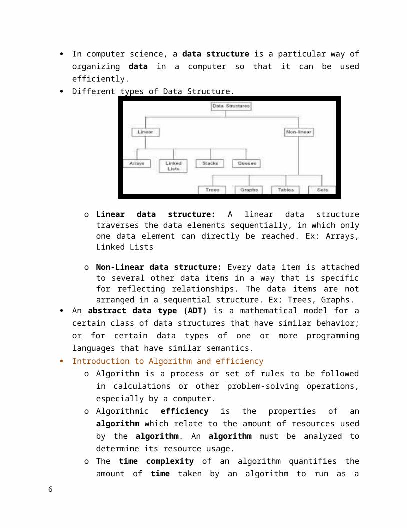
In computer science, a data structure is a particular way of organizing data in a computer so that it can be used efficiently.

Different types of Data Structure.

o Linear data structure: A linear data structure traverses the data elements sequentially, in which only one data element can directly be reached. Ex: Arrays, Linked Lists

o Non-Linear data structure: Every data item is attached to several other data items in a way that is specific for reflecting relationships. The data items are not arranged in a sequential structure. Ex: Trees, Graphs.

An abstract data type (ADT) is a mathematical model for a certain class of data structures that have similar behavior; or for certain data types of one or more programming languages that have similar semantics.

Introduction to Algorithm and efficiency o Algorithm is a process or set of rules to be followed in calculations or other

problem-solving operations, especially by a computer.o Algorithmic efficiency is the properties of an algorithm which relate to the

amount of resources used by the algorithm. An algorithm must be analyzed to determine its resource usage.

o The time complexity of an algorithm quantifies the amount of time taken by an algorithm to run as a function of the length of the string representing the input.

o Space Complexity of an algorithm is total space taken by the algorithm with respect to the input size. Space complexity includes both Auxiliary space and space used by input.

QuestionsWhat is ADT?What is linear and non linear data structure? Write the difference between them.

5

Lecture-4

Storage structure for arraysWhat is array?

C programming language provides a data structure called the array, which can store a fixed-size sequential collection of elements of the same type. An array is used to store a collection of data, but it is often more useful to think of an array as a collection of variables of the same type.

Instead of declaring individual variables, such as number0, number1, ..., and number99, you declare one array variable such as numbers and use numbers[0], numbers[1], and ..., numbers[99] to represent individual variables. A specific element in an array is accessed by an index.

All arrays consist of contiguous memory locations. The lowest address corresponds to the first element and the highest address to the last element.

Types of array.o Operations performed on linear array

o Traversal, Insertion, Deletion, Searching, Sorting and Merging.o Operations performed on 2D-array

Matrix addition and matrix multiplication.

Declaring Arrays

To declare an array in C, a programmer specifies the type of the elements and the number of elements required by an array as follows:

datatype arrayName [ arraySize ];

This is called a single-dimensional array. The array Size must be an integer constant greater than zero and type can be any valid C data type. For example, to declare a 10-element array called balance of type int, use this statement:

int balance[10];

Now balance is avariable array which is sufficient to hold up to 10 int numbers.

Initializing Arrays

You can initialize array in C either one by one or using a single statement as follows:

int balance[5] = {1000.0, 2.0, 3.4, 7.0, 50.0};

6

The number of values between braces { } cannot be larger than the number of elements that we declare for the array between square brackets [ ].

If you omit the size of the array, an array just big enough to hold the initialization is created. Therefore, if you write:

int balance[] = {1000.0, 2.0, 3.4, 7.0, 50.0};You will create exactly the same array as you did in the previous example. Following is an example to assign a single element of the array:

Balance [4] = 50.0;

The above statement assigns element number 5th in the array with a value of 50.0. All arrays have 0 as the index of their first element which is also called base index and last index of an array will be total size of the array minus 1.

Accessing Array Elements

An element is accessed by indexing the array name. This is done by placing the index of the element within square brackets after the name of the array. For example:

int salary = balance[9];

The above statement will take 10th element from the array and assign the value to salary variable.

Following is an example which will use all the above mentioned three concepts viz. declaration, assignment and accessing arrays:

#include <stdio.h> int main (){ int n[ 10 ]; /* n is an array of 10 integers */ int i,j; /* initialize elements of array n to 0 */ for ( i = 0; i < 10; i++ ) { n[ i ] = i + 100; /* set element at location i to i + 100 */ }

/* output each array element's value */ for (j = 0; j < 10; j++ ) { printf("Element[%d] = %d\n", j, n[j] ); } return 0;

7

}

Questions Objective

Consider an array a[10] of floats. if the base address of a is 100o,find the address of a[3]. Long Answer type-

Write a program to merge two arrays.Write a program to insert an element in an array.

8

Lecture-5

Sparse matrices What is sparse matrix?

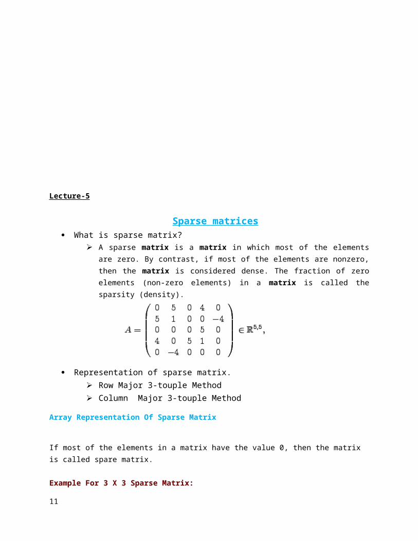
A sparse matrix is a matrix in which most of the elements are zero. By contrast, if most of the elements are nonzero, then the matrix is considered dense. The fraction of zero elements (non-zero elements) in a matrix is called the sparsity (density).

Representation of sparse matrix. Row Major 3-touple Method Column Major 3-touple Method

Array Representation Of Sparse Matrix

If most of the elements in a matrix have the value 0, then the matrix is called spare matrix.

Example For 3 X 3 Sparse Matrix: |  1   0   0 | |  0   0   0 | |  0   4   0 |

3-Tuple Representation Of Sparse Matrix:  |  3   3   2 | |  0   0   1 | |  2   1   4 |

Elements in the first row represents the number of rows, columns and non-zero values in sparse matrix.First Row  -  |  3   3   2 |3 - rows3 - columns2 - non- zero values

9

Elements in the other rows gives information about the location and value of non-zero elements.|  0   0   1 | ( Second Row) - represents value 1 at 0th Row, 0th column|  2   1   4 | (Third Row)     - represents value 4 at 2nd Row, 1st column

Sparse Matrix C program

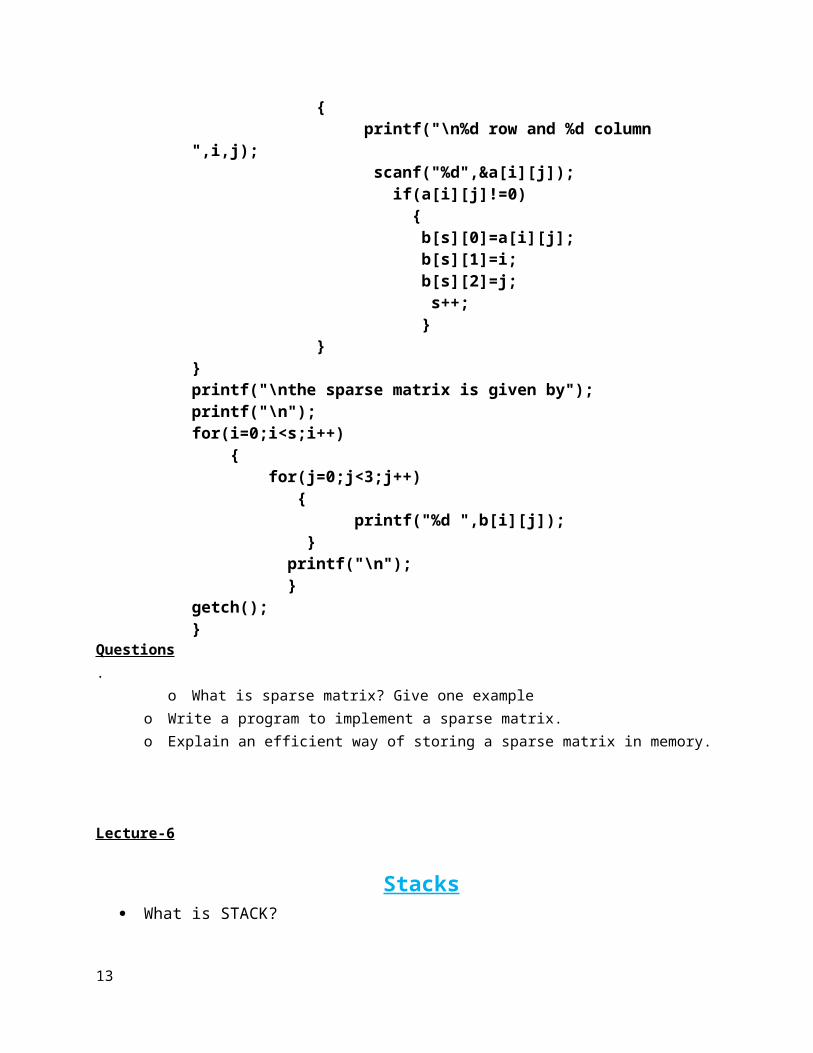
#include<stdio.h>#include<conio.h>void main(){ int a[10][10],b[10][3],r,c,s=0,i,j;clrscr();printf("\nenter the order of the sparse matrix");scanf("%d%d",&r,&c);printf("\nenter the elements in the sparse matrix(mostly zeroes)");for(i=0;i<r;i++) { for(j=0;j<c;j++) { printf("\n%d row and %d column ",i,j); scanf("%d",&a[i][j]); if(a[i][j]!=0) { b[s][0]=a[i][j]; b[s][1]=i; b[s][2]=j; s++; } }}printf("\nthe sparse matrix is given by");printf("\n");for(i=0;i<s;i++) { for(j=0;j<3;j++) { printf("%d ",b[i][j]); } printf("\n"); }getch();}

Questions.

o What is sparse matrix? Give one example

10

o Write a program to implement a sparse matrix.o Explain an efficient way of storing a sparse matrix in memory.

Lecture-6

Stacks What is STACK?

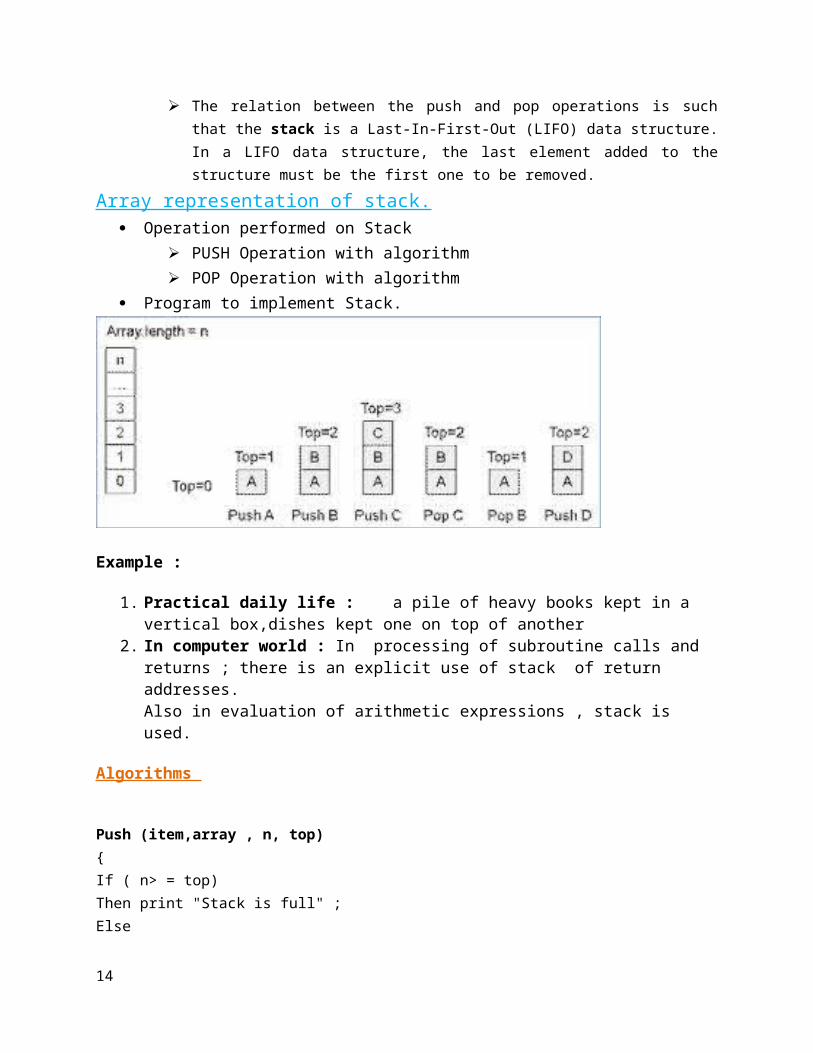
The relation between the push and pop operations is such that the stack is a Last-In-First-Out (LIFO) data structure. In a LIFO data structure, the last element added to the structure must be the first one to be removed.

Array representation of stack. Operation performed on Stack

PUSH Operation with algorithm POP Operation with algorithm

Program to implement Stack.

Example :

1. Practical daily life :    a pile of heavy books kept in a vertical box,dishes kept one on top of another

2. In computer world : In  processing of subroutine calls and returns ; there is an explicit use of stack  of return addresses.Also in evaluation of arithmetic expressions , stack is used. 

Algorithms

Push (item,array , n, top)   {If ( n> = top)  

11

Then print "Stack is full" ; Else top = top + 1; array[top] = item ;  }

Pop (item, array, top){ if ( top<= 0)Then print “stack is empty". Else item = array[top]; top = top – 1; } Questions

Objective o Which data structure used to perform recursion?o What is stack and how it can be represented using array.

Long Answer type- o Write down insert and delete algorithm of the stack using C-language notation with

proper example.o Reverse the order of element on a stack.

12

Lecture-7

Queues What is queue?

Definition of Queue. A queue is a data collection in which the items are kept in the order in which they were inserted, and the primary operations are enqueue (insert an item at the end) and dequeue (remove the item at the front).

Queues are also called “first-in first-out " (FIFO) list. Since the first element in a queue will be the first element out of the queue. In other words, the order in which elements enter in a queue is the order in which they leave. The real life example: the people waiting in a line at Railway ticket Counter form a queue, where the first person in a line is the first person to be waited on. An important example of a queue in computer science occurs in timesharing system, in which programs with the same priority form a queue while waiting to be executed.

Array representation of Queue. Different types of Queues

Linear queue, Dequeue, Circular queue, Priority Queue. Operation performed on Queue.

Traverse insertion, deletion operation and algorithm.

Example:

1. PRACTICAL EXAMPLE: A line at a ticket counter for buying tickets operates on above rules  

2. IN COMPUTER WORLD: In a batch processing system, jobs are queued up for processing.

13

Conditions in Queue

FRONT < 0 ( Queue is Empty ) REAR = Size of Queue ( Queue is Full ) FRONT < REAR ( Queue contains at least one element ) No of elements in queue is : ( REAR - FRONT ) + 1

Restriction in Queuewe cannot insert element directly at middle index (position) in Queue and vice verse for deletion. Insertion operation possible at REAR end only and deletion operation at FRONT end, to insert we increment REAR and to delete we increment FRONT.

Algorithm for ENQUEUE (insert element in Queue)

Input : An element say ITEM that has to be inserted.Output : ITEM is at the REAR of the Queue.Data structure: Que is an array representation of queue structure with two pointer FRONT and REAR.

Steps:

1.  If ( REAR = size ) then //Queue is full2.        print "Queue is full"3.        Exit4.  Else5.        If ( FRONT = 0 ) and ( REAR = 0 ) then //Queue is empty6.               FRONT = 17.        End if8.        REAR = REAR + 1 // increment REAR9.        Que[ REAR ] = ITEM10. End if11. Stop

Algorithm for DEQUEUE (delete element from Queue)

Input : A que with elements. FRONT and REAR are two pointer of queue .Output : The deleted element is stored in ITEM.Data structure : Que is an array representation of queue structure..

14

Steps:

1.  If ( FRONT = 0 ) then 2.        print "Queue is empty"3.        Exit4.  Else5.        ITEM = Que [ FRONT ]6.        If  ( FRONT  =  REAR )7.               REAR = 08.               FRONT = 09.        Else10.             FRONT  =  FRONT + 111.      End if12. End if 13. Stop 

//Program of Queue using array

# include<stdio.h># define MAX 5int queue_arr[MAX];int rear = -1;int front = -1;void insert();void del();void display();void main(){ int choice; while(1) { printf("1.Insert\n"); printf("2.Delete\n"); printf("3.Display\n"); printf("4.Quit\n"); printf("Enter your choice : "); scanf("%d",&choice); switch(choice) { case 1 : insert(); break; case 2 : del();

15

break; case 3: display(); break; case 4: exit(1); default: printf("Wrong choice\n"); } }}

void insert(){ int added_item; if (rear==MAX-1)

printf("Queue Overflow\n"); else { if (front==-1) /*If queue is initially empty */ front=0;

printf("Input the element for adding in queue : "); scanf("%d", &added_item);

rear=rear+1; queue_arr[rear] = added_item ; }}

void del(){ if (front == -1 || front > rear) { printf("Queue Underflow\n"); return ; } else { printf("Element deleted from queue is : %d\n", queue_arr[front]); front=front+1; }}

16

void display(){ int i; if (front == -1) printf("Queue is empty\n"); else { printf("Queue is :\n"); for(i=front;i<= rear;i++) printf("%d ",queue_arr[i]); printf("\n"); }}/*End of display() */

Questions Objective

o Difference between Stack and queue.o Define priority queue. Minimum number of queue needed to implement the priority

queue.

Long Answer type- o What is dequeue? Explain its two variant.o Develop a complete c-program to insert into and delete a node from an integer queue.

17

Lecture-8DE-Queue

The word dequeue is short form of double ended queue. In a dequeue , insertion as well as deletion can be carried out either at the rear end or the front end.

Operations on a Dequeue1. initialize(): Make the queue empty2. empty(): Determine if queue is empty3. full(): Determine if queue is full4. enqueueF(): Insert an element at the front end of the queue5. enqueueR(): Insert an element at the rear end of the queue6. dequeueR(): Delete the rear element7. dequeueF(): Delete the front element8. print(): Print elements of the queu

Circular Queue

Primary operations defined for a circular queue are:                 

1. Insert - It is used for addition of elements to the circular queue. 2. Delete - It is used for deletion of elements from the queue.

18

We will see that in a circular queue, unlike static linear array implementation of the queue ; the memory is utilized more efficient in case of circular queue's.

The shortcoming of static linear that once rear points to n which is the max size of our array we cannot insert any more elements even if there is space in the queue is removed efficiently using a circular queue.

As in case of linear queue, we'll see that condition for zero elements still remains the same i.e.. rear=front

ALGORITHM FOR ADDITION AND DELETION OF ELEMENTS

Data structures required for circular queue:

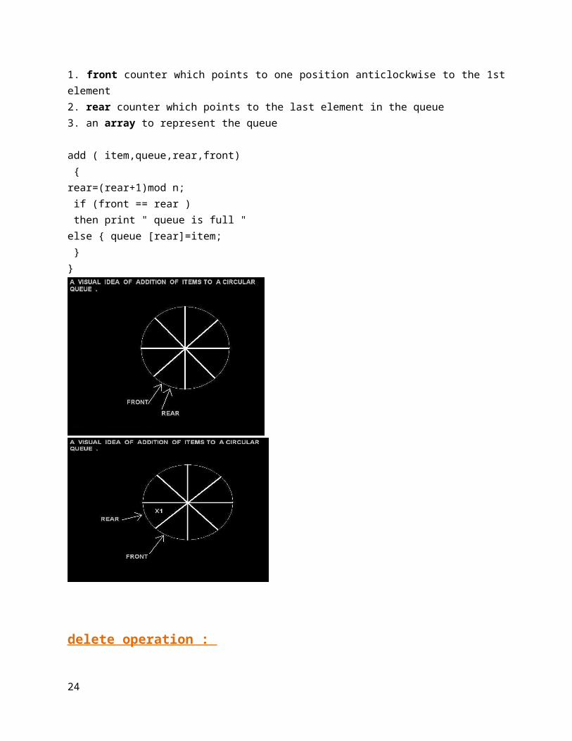
1. front counter which points to one position anticlockwise to the 1st element 2. rear counter which points to the last element in the queue 3. an array to represent the queue

add ( item,queue,rear,front) { rear=(rear+1)mod n;  if (front == rear )    then print " queue is full " else { queue [rear]=item; } }

19

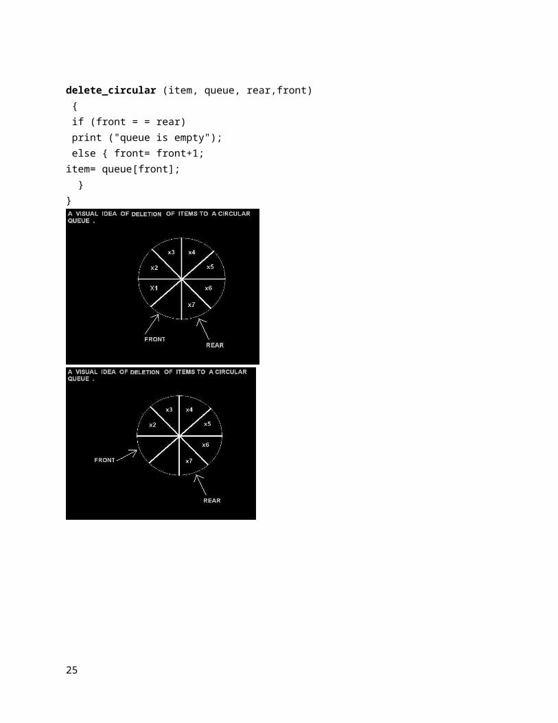
delete operation :

delete_circular (item, queue, rear,front) { if (front = = rear) print ("queue is empty"); else { front= front+1; item= queue[front];   } }

20

//Program of circular queue using array

# include<stdio.h># define MAX 5int cqueue_arr[MAX];int front = -1;

21

int rear = -1;

void insert();void del();void display();

void main(){ int choice; while(1) { printf("1.Insert\n"); printf("2.Delete\n"); printf("3.Display\n"); printf("4.Quit\n"); printf("Enter your choice : "); scanf("%d",&choice); switch(choice) { case 1 : insert(); break; case 2 : del(); break; case 3: display(); break; case 4: exit(1); default: printf("Wrong choice\n"); } }}

void insert(){ int added_item; if(front==(rear+1)%max) { printf("Queue Overflow \n"); return;

22

}else {rear=(rear+1)%max;printf("Input the element for insertion in queue : "); scanf("%d", &added_item); cqueue_arr[rear] = added_item ; if(f==-1)f=0; }void del(){ if (front ==rear== -1) { printf("Queue Underflow\n"); return ; } printf("Element deleted from queue is : %d\n",cqueue_arr[front]); if(front == rear) /* queue has only one element */ { front = -1; rear=-1; } else front=(front+1)%max;}

void display(){ int front_pos = front,rear_pos = rear; if(front == -1) { printf("Queue is empty\n"); return; } printf("Queue elements :\n"); if( front_pos <= rear_pos ) while(front_pos <= rear_pos) { printf("%d ",cqueue_arr[front_pos]); front_pos++;

23

} else { while(front_pos <= MAX-1) { printf("%d ",cqueue_arr[front_pos]); front_pos++; } front_pos = 0; while(front_pos <= rear_pos) { printf("%d ",cqueue_arr[front_pos]); front_pos++; } }

printf("\n");}

24

Lecture-9 PRIORITY QUEUE:

Often the items added to a queue have a priority associated with them: this priority determines the order in which they exit the queue - highest priority items are removed first.

This situation arises often in process control systems. Imagine the operator's console in a large automated factory. It receives many routine messages from all parts of the system: they are assigned a low priority because they just report the normal functioning of the system - they update various parts of the operator's console display simply so that there is some confirmation that there are no problems. It will make little difference if they are delayed or lost.

However, occasionally something breaks or fails and alarm messages are sent. These have high priority because some action is required to fix the problem (even if it is mass evacuation because nothing can stop the imminent explosion!). Typically such a system will be composed of many small units, one of which will be a buffer for messages received by the operator's console. The communications system places messages in the buffer so that communications links can be freed for further messages while the console software is processing the message. The console software extracts messages from the buffer and updates appropriate parts of the display system. Obviously we want to sort messages on their priority so that we can ensure that the alarms are processed immediately and not delayed behind a few thousand routine messages while the plant is about to explode

Application of stack and queue Application of stack

Implementation of recursion. Evaluation of arithmetic expression

25

Conversion of infix infix to postfix expression Evaluation of postfix expression

Application of queue Introduuction to breadth first search graph. Time sharing computer system. Introduction to simulation.

Lecture-10Linked lists: Single linked lists

What is a Linked Lists?

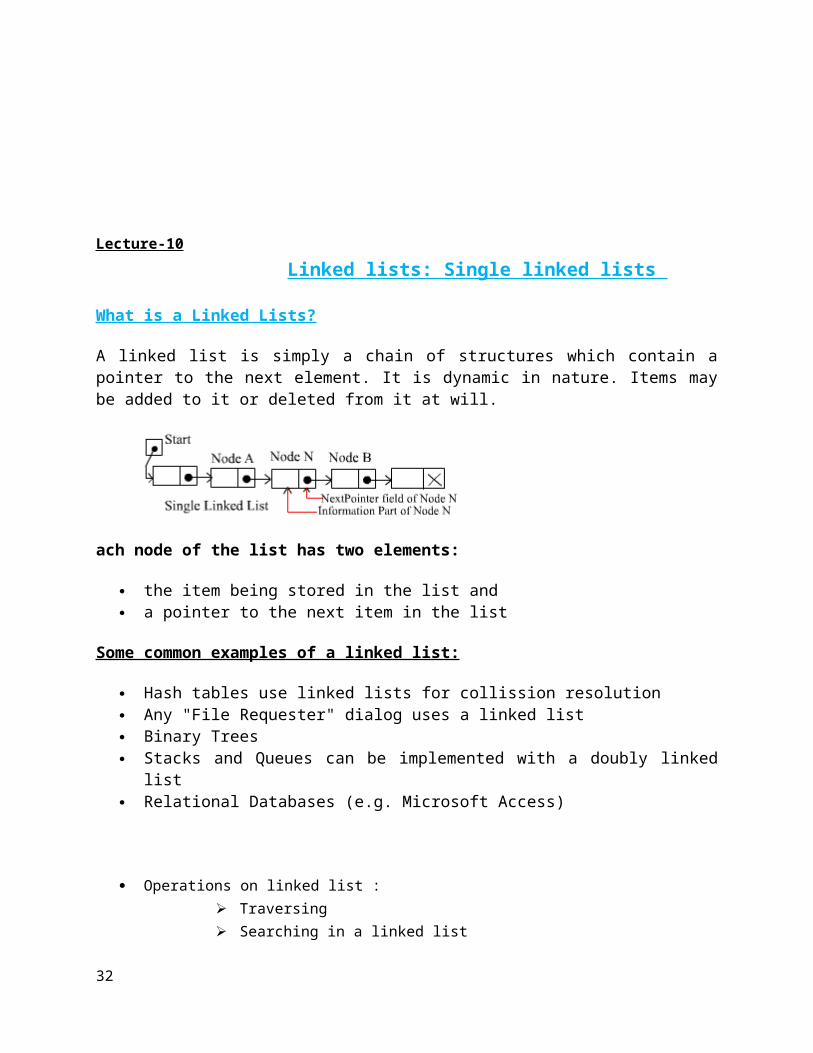
A linked list is simply a chain of structures which contain a pointer to the next element. It is dynamic in nature. Items may be added to it or deleted from it at will. 

ach node of the list has two elements:

the item being stored in the list and a pointer to the next item in the list

Some common examples of a linked list:

Hash tables use linked lists for collission resolution Any "File Requester" dialog uses a linked list Binary Trees Stacks and Queues can be implemented with a doubly linked list Relational Databases (e.g. Microsoft Access)

Operations on linked list : Traversing Searching in a linked list

26

o Sortedo Unsorted

Types of Link List

1. Linearly-linked List o Singly-linked list o Doubly-linked list

2. Circularly-linked list o Singly-circularly-linked listo Doubly-circularly-linked list

3. Sentinel node.

Lecture-11

Operations on Linked lists Insertion

Insert at the beginning Insert at the end Insert after a given node

Deletion Delete the first node \Delete the last node Delete a particular node

Algorithm for inserting   a node to the List

allocate space for a new node, copy the item into it, make the new node's next pointer point to the current head of the list and Make the head of the list point to the newly allocated node.

This strategy is fast and efficient, but each item is added to the head of the list. Below is given C code for inserting a node after a given nod

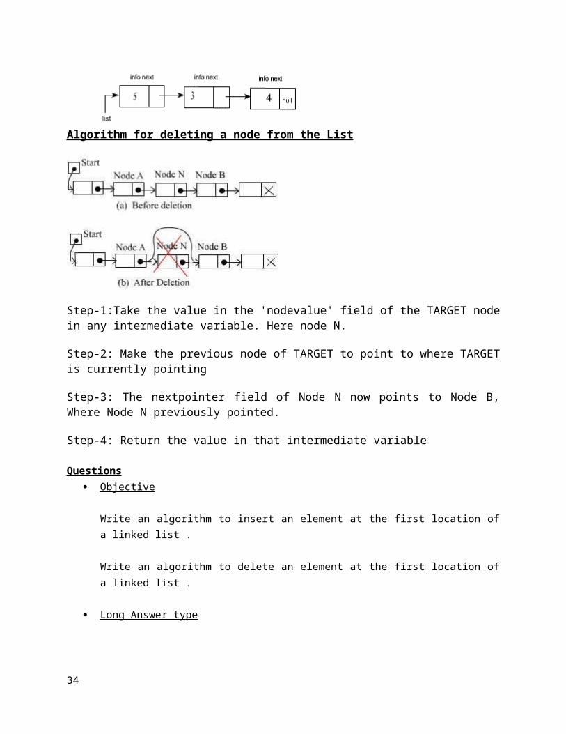
Algorithm for deleting a node from the List

27

Step-1:Take the value in the 'nodevalue' field of the TARGET node in any intermediate variable. Here node N.

Step-2: Make the previous node of TARGET to point to where TARGET is currently pointing

Step-3: The nextpointer field of Node N now points to Node B, Where Node N previously pointed.

Step-4: Return the value in that intermediate variable

Questions Objective

Write an algorithm to insert an element at the first location of a linked list .

Write an algorithm to delete an element at the first location of a linked list .

Long Answer type

1. Write an algorithm to insert a node to a single linked list by taking the position from the user. The position can be first, last or any other position between these two.

2. Write an algorithm to delete a node of a single linked list by taking the position from the user. The position can be first, last or any other position between these two.

//Program of single linked list# include <stdio.h># include <malloc.h>struct node{ int info; struct node *link;}*start;main()

28

{ int choice,n,m,position,i; start=NULL; while(1) { printf("1.Create List\n"); printf("2.Add at begining\n"); printf("3.Add after \n"); printf("4.Delete\n"); printf("5.Display\n"); printf("6.Count\n"); printf("7.Reverse\n"); printf("8.Search\n"); printf("9.Quit\n"); printf("Enter your choice : "); scanf("%d",&choice); switch(choice) { case 1: printf("How many nodes you want : "); scanf("%d",&n); for(i=0;i<n;i++) { printf("Enter the element : "); scanf("%d",&m); create_list(m); } break; case 2: printf("Enter the element : "); scanf("%d",&m); addatbeg(m); break; case 3: printf("Enter the element : "); scanf("%d",&m); printf("Enter the position after which this element is inserted : "); scanf("%d",&position); addafter(m,position); break; case 4: if(start==NULL) { printf("List is empty\n"); continue; } printf("Enter the element for deletion : ");

29

scanf("%d",&m); del(m); break; case 5: display(); break; case 6: count(); break; case 7: rev(); break; case 8: printf("Enter the element to be searched : "); scanf("%d",&m); search(m); break; case 9: exit(); default: printf("Wrong choice\n"); }/*End of switch */ }/*End of while */}/*End of main()*/

create_list(int data){ struct node *q,*temp; temp= malloc(sizeof(struct node)); temp->info=data; temp->link=NULL; if(start==NULL) /*If list is empty */ start=temp; else { /*Element inserted at the end */ q=start; while(q->link!=NULL) q=q->link; q->link=temp; }}/*End of create_list()*/addatbeg(int data){ struct node *temp;

30

temp=malloc(sizeof(struct node)); temp->info=data; temp->link=start; start=temp;}/*End of addatbeg()*/

addafter(int data,int pos){ struct node *temp,*q; int i; q=start; for(i=0;i<pos-1;i++) { q=q->link; if(q==NULL) { printf("There are less than %d elements",pos); return; } }/*End of for*/ temp=malloc(sizeof(struct node) ); temp->link=q->link; temp->info=data; q->link=temp;}/*End of addafter()*/del(int data){ struct node *temp,*q; if(start->info == data) { temp=start; start=start->link; /*First element deleted*/ free(temp); return; } q=start; while(q->link->link != NULL) { if(q->link->info==data) /*Element deleted in between*/ {

31

temp=q->link; q->link=temp->link; free(temp); return; } q=q->link; }/*End of while */ if(q->link->info==data) /*Last element deleted*/ { temp=q->link; free(temp); q->link=NULL; return; } printf("Element %d not found\n",data);}/*End of del()*/display(){ struct node *q; if(start == NULL) { printf("List is empty\n"); return; } q=start; printf("List is :\n"); while(q!=NULL) { printf("%d ", q->info); q=q->link; } printf("\n");}/*End of display() */count(){ struct node *q=start; int cnt=0; while(q!=NULL) { q=q->link; cnt++; } printf("Number of elements are %d\n",cnt);}/*End of count() */

32

rev(){ struct node *p1,*p2,*p3; if(start->link==NULL) /*only one element*/ return; p1=start; p2=p1->link; p3=p2->link; p1->link=NULL; p2->link=p1; while(p3!=NULL) { p1=p2; p2=p3; p3=p3->link; p2->link=p1; } start=p2;}/*End of rev()*/search(int data){ struct node *ptr = start; int pos = 1; while(ptr!=NULL) { if(ptr->info==data) { printf("Item %d found at position %d\n",data,pos); return; } ptr = ptr->link; pos++; } if(ptr == NULL)printf("Item %d not found in list\n",data);}/*End of search()*/

33

Lecture-12

Linked list representation of stacks

The operation of adding an element to the front of a linked list is quite similar to that of pushing an element on to a stack. A stack can be accessed only through its top element, and a list can be accessed only from the pointer to its first element. Similarly, removing the first element from a linked list is analogous to popping from a stack.

A linked-list is somewhat of a dynamic array that grows and shrinks as values are added to it and removed from it respectively. Rather than being stored in a continuous block of memory, the values in the dynamic array are linked together with pointers. Each element of a linked list is a structure that contains a value and a link to its neighbor. The link is basically a pointer to another structure that contains a value and another pointer to another structure, and so on. If an external pointer p points to such a linked list, the operation push(p, t) may be implemented by

Program

#include <stdio.h>#include <stdlib.h> struct node{ int info; struct node *ptr;}*top,*top1,*temp; int topelement();void push(int data);

34

void pop();void empty();void display();void destroy();void stack_count();void create(); int count = 0; void main(){ int no, ch, e;  printf("\n 1 - Push"); printf("\n 2 - Pop"); printf("\n 3 - Top"); printf("\n 4 - Empty"); printf("\n 5 - Exit"); printf("\n 6 - Dipslay"); printf("\n 7 - Stack Count"); printf("\n 8 - Destroy stack");  create();  while (1) { printf("\n Enter choice : "); scanf("%d", &ch);  switch (ch) { case 1: printf("Enter data : "); scanf("%d", &no); push(no); break; case 2: pop(); break; case 3: if (top == NULL) printf("No elements in stack"); else { e = topelement(); printf("\n Top element : %d", e);

35

} break; case 4: empty(); break; case 5: exit(0); case 6: display(); break; case 7: stack_count(); break; case 8: destroy(); break; default : printf(" Wrong choice, Please enter correct choice "); break; } }} /* Create empty stack */void create(){ top = NULL;} /* Count stack elements */void stack_count(){ printf("\n No. of elements in stack : %d", count);} /* Push data into stack */void push(int data){ if (top == NULL) { top =(struct node *)malloc(1*sizeof(struct node)); top->ptr = NULL; top->info = data; } else {

36

temp =(struct node *)malloc(1*sizeof(struct node)); temp->ptr = top; temp->info = data; top = temp; } count++;} /* Display stack elements */void display(){ top1 = top;  if (top1 == NULL) { printf("Stack is empty"); return; }  while (top1 != NULL) { printf("%d ", top1->info); top1 = top1->ptr; } } /* Pop Operation on stack */void pop(){ top1 = top;  if (top1 == NULL) { printf("\n Error : Trying to pop from empty stack"); return; } else top1 = top1->ptr; printf("\n Popped value : %d", top->info); free(top); top = top1; count--;} /* Return top element */int topelement()

37

{ return(top->info);} /* Check if stack is empty or not */void empty(){ if (top == NULL) printf("\n Stack is empty"); else printf("\n Stack is not empty with %d elements", count);} /* Destroy entire stack */void destroy(){ top1 = top;  while (top1 != NULL) { top1 = top->ptr; free(top); top = top1; top1 = top1->ptr; } free(top1); top = NULL;  printf("\n All stack elements destroyed"); count = 0;}

38

Lecture-14

Linked list representation of Queue

Linked Implementation of Queue Queues can be implemented as linked lists. Linked list implementations of queues often require two pointers or references to links at the beginning and end of the list. Using a pair of pointers or references opens the code up to a variety of bugs especially when the last item on the queue is dequeued or when the first item is enqueued.

In a circular linked list representation of queues, ordinary 'for loops' and 'do while loops' do not suffice to traverse a loop because the link that starts the traversal is also the link that terminates the traversal. The empty queue has no links and this is not a circularly linked list. This is also a problem for the two pointers or references approach. If one link in the circularly linked queue is kept empty then traversal is simplified. The one empty link simplifies traversal since the traversal starts on the first link and ends on the empty one. Because there will always be at least one link on the queue (the empty one) the queue will always be a circularly linked list and no bugs will arise from the queue being intermittently circular. Let a pointer to the first element of a list represent the front of the queue. Another pointer to the last element of the list represents the rear of the queue as shown in fig. illustrates the same queue after a new item has been inserted.

Program

39

#include <stdio.h>#include <stdlib.h> struct node{ int info; struct node *ptr;}*front,*rear,*temp,*front1; int frontelement();void enq(int data);void deq();void empty();void display();void create();void queuesize(); int count = 0; void main(){ int no, ch, e;  printf("\n 1 - Enque"); printf("\n 2 - Deque"); printf("\n 3 - Front element"); printf("\n 4 - Empty"); printf("\n 5 - Exit"); printf("\n 6 - Display"); printf("\n 7 - Queue size"); create(); while (1) { printf("\n Enter choice : "); scanf("%d", &ch); switch (ch) { case 1: printf("Enter data : "); scanf("%d", &no); enq(no); break; case 2: deq(); break;

40

case 3: e = frontelement(); if (e != 0) printf("Front element : %d", e); else printf("\n No front element in Queue as queue is empty"); break; case 4: empty(); break; case 5: exit(0); case 6: display(); break; case 7: queuesize(); break; default: printf("Wrong choice, Please enter correct choice "); break; } }} /* Create an empty queue */void create(){ front = rear = NULL;} /* Returns queue size */void queuesize(){ printf("\n Queue size : %d", count);} /* Enqueing the queue */void enq(int data){ if (rear == NULL) { rear = (struct node *)malloc(1*sizeof(struct node)); rear->ptr = NULL; rear->info = data; front = rear;

41

} else { temp =(struct node *)malloc(1*sizeof(struct node)); rear->ptr = temp; temp->info = data; temp->ptr = NULL;  rear = temp; } count++;} /* Displaying the queue elements */void display(){ front1 = front;  if ((front1 == NULL) && (rear == NULL)) { printf("Queue is empty"); return; } while (front1 != rear) { printf("%d ", front1->info); front1 = front1->ptr; } if (front1 == rear) printf("%d", front1->info);} /* Dequeing the queue */void deq(){ front1 = front;  if (front1 == NULL) { printf("\n Error: Trying to display elements from empty queue"); return; } else if (front1->ptr != NULL) { front1 = front1->ptr;

42

printf("\n Dequed value : %d", front->info); free(front); front = front1; } else { printf("\n Dequed value : %d", front->info); free(front); front = NULL; rear = NULL; } count --;} /* Returns the front element of queue */int frontelement(){ if ((front != NULL) && (rear != NULL)) return (front->info); else return 0;} /* Display if queue is empty or not */void empty(){ if ((front == NULL) && (rear == NULL)) printf("\n Queue empty"); else printf("Queue not empty");}

43

Lecture-15Operations on polynomials

Let us now see how two polynomials can be added. Let P1 and P2 be two polynomials stored as linked lists in sorted (decreasing) order of exponents The addition operation is defined as follows. Add terms of like-exponents. We have P1 and P2 arranged in a linked list in decreasing order of exponents. We can scan these and add like terms. Need to store the resulting term only if it has non-zero coefficient. The number of terms in the result polynomial P1+P2 need not be known in advance. We'll use as much space as there are terms in P1+P2. 

Adding polynomials :(3x5 – 9x3 + 4x2) + (–8x5 + 8x3 + 2)= 3x5 – 8x5 – 9x3 + 8x3 + 4x2 + 2= –5x5 – x3 + 4x2 + 2 

Multiplying polynomials:(2x – 3)(2x2 + 3x – 2)= 2x(2x2 + 3x – 2) – 3(2x2 + 3x – 2)= 4x3 + 6x2 – 4x – 6x2 – 9x+ 6= 4x3 – 13x+ 6

Application - Polynomials

  Application of linked lists is to polynomials. We now use linked lists to perform

operations on polynomials. Let f(x) = Σdi=0 aixi. The quantity d is called as the degree of the polynomial, with the assumption that ad not equal to 0. A polynomial of degree d may however have missing terms i.e., powers j such that 0 <= j < d and aj = 0.The standard operations on a polynomial are addition and multiplication. If we store the coefficient of each term of the polynomials in an array of size d + 1, then these operations can be supported in a straight forward way. However, for sparse polynomails, i.e., polynomials where there are few non-zero coefficients, this is not efficient. One possible solution is to use linked lists to store degree, coefficient pairs for non-zero coefficients. With this

44

representation, it makes it easier if we keep the list of such pairs in decreasing order of degrees. 

A polynomial is a sum of terms. Each term consists of a coefficient and a (common) variable raised to an exponent. We consider only integer exponents, for now.

o Example: 4x3 + 5x – 10. How to represent a polynomial? Issues in representation, should not waste space, should

be easy to use it for operating on polynomials. Any case, we need to store the coefficient and the exponent.

struct node{float coefficient;int exponent;struct node *next;}

Questions Objective

Find the minimum number of multiplications and additions required to evaluate the polynomial P=4x3+3 x2-15x+45

Long Answer type

Write an algorithm to add two polynomials?

45

Lecture-16

Doubly linked list

In computer science, a doubly-linked list is a linked data structure that consists of a set of sequentially linked records called nodes. Each node contains two fields, called links, that are references to the previous and to the next node in the sequence of nodes. The beginning and ending nodes' previous and next links, respectively, point to some kind of terminator, typically a sentinel node or null, to facilitate traversal of the list. If there is only one sentinel node, then the list is circularly linked via the sentinel node. It can be conceptualized as two singly linked lists formed from the same data items, but in opposite sequential orders.

A doubly-linked list whose nodes contain three fields: an integer value, the link to the next node, and the link to the previous node.

The two node links allow traversal of the list in either direction. While adding or removing a node in a doubly-linked list requires changing more links than the same operations on a singly linked list, the operations are simpler and potentially more efficient (for nodes other than first nodes) because there is no need to keep track of the previous node during traversal or no need to traverse the list to find the previous node, so that its link can be modified.

Doubly linked lists are like singly linked lists, in which for each node there are two pointers -- one to the next node, and one to the previous node. This makes life nice in many ways:

You can traverse lists forward and backward.

46

You can insert anywhere in a list easily. This includes inserting before a node, after a node, at the front of the list, and at the end of the list and

You can delete nodes very easily.

Doubly linked lists may be either linear or circular and may or may not contain a header node

Lecture-17

Operations on double linked list : Traversing

Insertion Insert at the beginning Insert at the end Insert after a given node

Deletion Delete the first node Delete the last node Delete a particular node

Questions Objective

What are the advantage of two way linked list over single linked list ? Long Answer type

Write an algorithm to insert a node to a double linked list by taking the position from the user. The position can be first, last or any other position between these two.

Write an algorithm to delete a node of a double linked list by taking the position from the user. The position can be first , last or any other position between these two.

Program of double linked list# include <stdio.h># include <malloc.h>struct node{ struct node *prev;

47

int info; struct node *next;}*start;void main(){ int choice,n,m,po,i; start=NULL; while(1) { printf("1.Create List\n"); printf("2.Add at begining\n"); printf("3.Add after\n"); printf("4.Delete\n"); printf("5.Display\n"); printf("6.Count\n"); printf("7.Reverse\n"); printf("8.exit\n"); printf("Enter your choice : "); scanf("%d",&choice); switch(choice) { case 1: printf("How many nodes you want : "); scanf("%d",&n); for(i=0;i<n;i++) { printf("Enter the element : "); scanf("%d",&m); create_list(m); } break; case 2: printf("Enter the element : "); scanf("%d",&m); addatbeg(m); break; case 3: printf("Enter the element : "); scanf("%d",&m); printf("Enter the position after which this element is inserted : "); scanf("%d",&po); addafter(m,po); break; case 4:

48

printf("Enter the element for deletion : "); scanf("%d",&m); del(m); break; case 5: display(); break; case 6: count(); break; case 7: rev(); break; case 8: exit(); default: printf("Wrong choice\n"); }/*End of switch*/ }/*End of while*/}/*End of main()*/

create_list(int num){ struct node *q,*temp; temp= malloc(sizeof(struct node)); temp->info=num; temp->next=NULL; if(start==NULL) { temp->prev=NULL; start->prev=temp; start=temp; } else { q=start; while(q->next!=NULL) q=q->next; q->next=temp; temp->prev=q; }}/*End of create_list()*/

addatbeg(int num)

49

{ struct node *temp; temp=malloc(sizeof(struct node)); temp->prev=NULL; temp->info=num; temp->next=start; start->prev=temp; start=temp;}/*End of addatbeg()*/addafter(int num,int c){ struct node *temp,*q; int i; q=start; for(i=0;i<c-1;i++) { q=q->next; if(q==NULL) { printf("There are less than %d elements\n",c); return; } } temp=malloc(sizeof(struct node) ); temp->info=num; q->next->prev=temp; temp->next=q->next; temp->prev=q; q->next=temp;}/*End of addafter() */

del(int num){ struct node *temp,*q; if(start->info==num) { temp=start; start=start->next; /*first element deleted*/ start->prev = NULL; free(temp); return; } q=start; while(q->next->next!=NULL) { if(q->next->info==num) /*Element deleted in between*/

50

{ temp=q->next; q->next=temp->next; temp->next->prev=q; free(temp); return; } q=q->next; } if(q->next->info==num) /*last element deleted*/ { temp=q->next; free(temp); q->next=NULL; return; } printf("Element %d not found\n",num);}/*End of del()*/

display(){ struct node *q; if(start==NULL) { printf("List is empty\n"); return; } q=start; printf("List is :\n"); while(q!=NULL) { printf("%d ", q->info); q=q->next; } printf("\n");}/*End of display() */

count(){ struct node *q=start; int cnt=0; while(q!=NULL) { q=q->next;

51

cnt++; } printf("Number of elements are %d\n",cnt);}/*End of count()*/

rev(){ struct node *p1,*p2; p1=start; p2=p1->next; p1->next=NULL; p1->prev=p2; while(p2!=NULL) { p2->prev=p2->next; p2->next=p1; p1=p2; p2=p2->prev; /*next of p2 changed to prev */ } start=p1;}/*End of rev()*/

52

Lecure-18

CIRCULAR   LIST          

Circular lists are like singly linked lists, except that the last node contains a  pointer back to the first node rather than the null pointer. From any point in such a list, it is possible to reach any other point in the list. If we begin at a given node and travel the entire list, we ultimately end up at the starting point.

Note that a circular list does not have a natural "first or "last" node. We must therefore, establish a first and last node by convention - let external pointer point to the last node, and the following node be the first node.

Single circular linked list Double circular linked list

Header Nodes

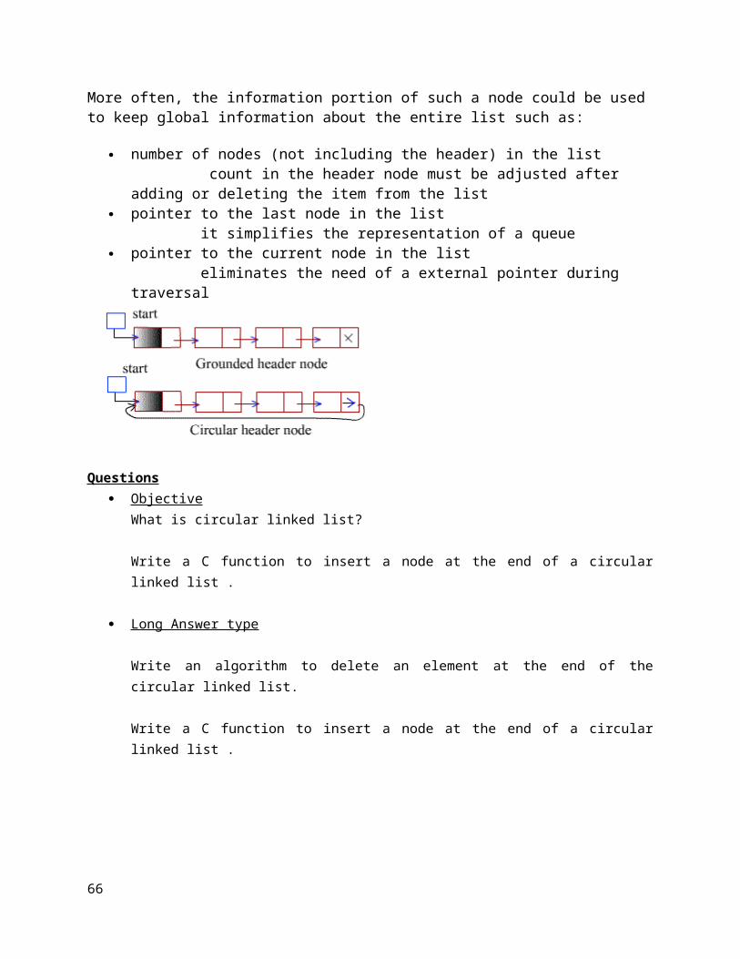
A header linked list is a linked list which always contains a special node called the header node at the beginning of the list. It is an extra node kept at the front of a list. Such a node does not represent an item in the list. The information portion might be unused. There are two types of header list

1. Grounded header list: is a header list where the last node contain the null pointer.2. Circular header list: is a header list where the last node points back to the header node.

More often, the information portion of such a node could be used to keep global information about the entire list such as:

number of nodes (not including the header) in the list          count in the header node must be adjusted after adding or deleting the item from the list

pointer to the last node in the list         it simplifies the representation of a queue

53

pointer to the current node in the list         eliminates the need of a external pointer during traversal

 

Questions Objective

What is circular linked list?

Write a C function to insert a node at the end of a circular linked list .

Long Answer type

Write an algorithm to delete an element at the end of the circular linked list.

Write a C function to insert a node at the end of a circular linked list .

54

Module – II

Dynamic storage management-garbage collection and compaction, infix to post fix conversion, postfix expression evaluation. Trees: Tree terminology, Binary tree, Binary search tree, General tree, B+ tree, AVL Tree, Complete Binary Tree representation, Tree traversals, operation on Binary tree-expression Manipulation.

55

Lecture-19

Dynamic storage management

Memory management is the act of managing computer memory at the system level. The essential requirement of memory management is to provide ways to dynamically allocate portions of memory to programs at their request, and free it for reuse when no longer needed. This is critical to any advanced computer system where more than a single process might be underway at any time.

Several methods have been devised that increase the effectiveness of memory management. Virtual memory systems separate the memory addresses used by a process from actual physical addresses, allowing separation of processes and increasing the effectively available amount of RAM using paging or swapping to secondary storage. The quality of the virtual memory manager can have an extensive effect on overall system performance.

Static Memory Management:

When memory is allocated during compilation time, it is called ‘Static Memory Management’. This memory is fixed and cannot be increased or decreased after allocation. If more memory is allocated than requirement, then memory is wasted. If less memory is allocated than requirement, then program will not run successfully. So exact memory requirements must be known in advance.

Dynamic Memory Management:

When memory is allocated during run/execution time, it is called ‘Dynamic Memory Management’. This memory is not fixed and is allocated according to our requirements. Thus in it there is no wastage of memory. So there is no need to know exact memory requirements in advance.

56

Two basic operations in dynamic storage management: Allocate a given number of bytes Free a previously allocated block

Two general approaches to dynamic storage allocation: Stack allocation (hierarchical): restricted, but simple and efficient. Heap allocation: more general, but less efficient, more difficult to implement.

Fixed-size blocks allocation

Fixed-size blocks allocation, also called memory pool allocation, uses a free list of fixed-size blocks of memory (often all of the same size). This works well for simple embedded systems where no large objects need to be allocated, but suffers from fragmentation, especially with long memory addresses. However, due to the significantly reduced overhead this method can substantially improve performance for objects that need frequent allocation / de-allocation and is often used in video games.

Buddy blocks

In this system, memory is allocated into several pools of memory instead of just one, where each pool represents blocks of memory of a certain power of two in size. All blocks of a particular size are kept in a sorted linked list or tree and all new blocks that are formed during allocation are added to their respective memory pools for later use. If a smaller size is requested than is available, the smallest available size is selected and halved. One of the resulting halves is selected, and the process repeats until the request is complete. When a block is allocated, the allocator will start with the smallest sufficiently large block to avoid needlessly breaking blocks. When a block is freed, it is compared to its buddy. If they are both free, they are combined and placed in the next-largest size buddy-block list.

The exact size of array is unknown untill the compile time,i.e., time when a compier compiles code written in a programming language into a executable form. The size of array you have declared initially can be sometimes insufficient and sometimes more than required. Dynamic memory allocation allows a program to obtain more memory space, while running or to release space when no space is required.

Although, C language inherently does not has any technique to allocated memory dynamically, there are 4 library functions under "stdlib.h" for dynamic memory allocation.

Function Use of Function

malloc() Allocates requested size of bytes and returns a pointer first byte of allocated space

calloc()Allocates space for an array elements, initializes to zero and then returns a pointer to memory

57

Function Use of Function

free() dellocate the previously allocated space

realloc() Change the size of previously allocated space

malloc()

The name malloc stands for "memory allocation". The function malloc() reserves a block of memory of specified size and return a pointer of type void which can be casted into pointer of any form.

Syntax of malloc()ptr=(cast-type*)malloc(byte-size)

Here, ptr is pointer of cast-type. The malloc() function returns a pointer to an area of memory with size of byte size. If the space is insufficient, allocation fails and returns NULL pointer.

ptr=(int*)malloc(100*sizeof(int));

This statement will allocate either 200 or 400 according to size of int 2 or 4 bytes respectively and the pointer points to the address of first byte of memory.

calloc()

The name calloc stands for "contiguous allocation". The only difference between malloc() and calloc() is that, malloc() allocates single block of memory whereas calloc() allocates multiple blocks of memory each of same size and sets all bytes to zero.

Syntax of calloc()ptr=(cast-type*)calloc(n,element-size);

This statement will allocate contiguous space in memory for an array of n elements. For example:

ptr=(float*)calloc(25,sizeof(float));

This statement allocates contiguous space in memory for an array of 25 elements each of size of float, i.e, 4 bytes.

free()

Dynamically allocated memory with either calloc() or malloc() does not get return on its own. The programmer must use free() explicitly to release space.

58

syntax of free()free(ptr);

This statement causes the space in memory pointer by ptr to be deallocated.

Examples of calloc() and malloc()

Write a C program to find sum of n elements entered by user. To perform this program, allocate memory dynamically using malloc() function.

#include <stdio.h>#include <stdlib.h>int main(){ int n,i,*ptr,sum=0; printf("Enter number of elements: "); scanf("%d",&n); ptr=(int*)malloc(n*sizeof(int)); //memory allocated using malloc if(ptr==NULL) { printf("Error! memory not allocated."); exit(0); } printf("Enter elements of array: "); for(i=0;i<n;++i) { scanf("%d",ptr+i); sum+=*(ptr+i); } printf("Sum=%d",sum); free(ptr); return 0;}

Questions

Objective What is the use of dynamic storage management?

Short notes on dynamic storage management

What is the difference between malloc( ) and calloc( )

59

Lecture-20

Garbage Collection and compaction

Manual Storage Management vs. Automatic Garbage Collection

There are two basic strategies for dealing with garbage: manual storage management by the programmer and automatic garbage collection built into the language run-time system. Language constructs for manual storage management are provided by languages like C and C++. There is a way for the programmer to explicitly allocate blocks of memory when needed and to deallocate (or "free") them when they become garbage. Languages like Java and OCaml provide automatic garbage collection: the system automatically identifies blocks of memory that can never be used again by the program and reclaims their space for later use.

Automatic garbage collection offers the advantage that the programmer does not have to worry about when to deallocate a given block of memory. In languages like C, the need to manage memory explicitly complicates any code that allocates data on the heap and is a significant burden on the programmer, not to mention a major source of bugs:

If the programmer neglects to deallocate garbage, it creates a memory leak in which some allocated memory can never again be reused. This is a problem for long-running programs, such as operating systems. Over time, the unreclaimable garbage grows in size until it consumes all of memory, at which point the system crashes.

If the programmer accidentally deallocates a block of memory that is still in use, this creates a dangling pointer that may be followed later, even though it now points to unallocated memory or to a new allocated value that may be of a different type.

If a block of memory is accidentally deallocated twice, this typically corrupts the memory heap data structure even if the block was initially garbage. Corruption of the memory heap is likely to cause unpredictable effects later during execution and is extremely difficult to debug.

60

In practice, programmers manage explicit allocation and deallocation by keeping track of what piece of code "owns" each pointer in the system. That piece of code is responsible for deallocating the pointer later. The tracking of pointer ownership shows up in the specifications of code that manipulates pointers, complicating specification, use, and implementation of the abstraction.

Automatic garbage collection helps modular programming, because two modules can share a value without having to agree on which module is responsible for deallocating it.

Requirements for Automatic Garbage Collection

The following properties are desirable in a garbage collector:

It should identify most garbage. Anything it identifies as garbage must be garbage. It should impose a low added time overhead. During garbage collection, the program may be paused, but these pauses should be short.

Fortunately, modern garbage collectors provide all of these important properties. We will not have time for a complete survey of modern garbage collection techniques, but we can look at some simple garbage collectors.

Identifying Pointers

To compute reachability accurately, the garbage collector needs to be able to identify pointers; that is, the edges in the graph. Since a word of memory cells is just a sequence of bits, how can the garbage collector tell apart a pointer from an integer? One simple strategy is to reserve a bit in every word to indicate whether the value in that word is a pointer or not. This tag bit uses up about 3% of memory, which may be acceptable. It also limits the range of integers (and pointers) that can be used. On a 32-bit machines, using a single tag bit means that integers can go up to about 1 billion, and that the machine can address about 2GB instead of the 4GB that would otherwise be possible. Adding tag bits also introduces a small run-time cost that is incurred during arithmetic or when dereferencing a pointer.

A different solution is to have the compiler record information that the garbage collector can query at run time to find out the types of the various locations on the stack. Given the types of stack locations, the successive pointers can be followed from these roots and the types used at every step to determine where the pointers are. This approach avoids the need for tag bits but is substantially more complicated because the garbage collector and the compiler become more tightly coupled.

Finally, it is possible to build a garbage collector that works even if you can't tell apart pointers and integers. The idea is that if the collector encounters something that looks like it might be a pointer, it treats it as if it is one, and the memory block it points to is treated as reachable. Memory is considered unreachable only if there is nothing that looks like it might be a pointer to it. This kind of collector is called a conservative collector because it may fail to collect some

61

garbage, but it won't deallocate anything but garbage. In practice it works pretty well because most integers are small and most pointers look like large integers. So there are relatively few cases in which the collector is not sure whether a block of memory is garbage.

Mark and Sweep Collection

Mark-and-sweep proceeds in two phases: a mark phase in which all reachable memory is marked as reachable, and a sweep phase in which all memory that has not been marked is deallocated. This algorithm requires that every block of memory have a bit reserved in it to indicate whether it has been marked.

Marking for reachability is essentially a graph traversal; it can be implemented as either a depth-first or a breadth-first traversal. One problem with a straightforward implementation of marking is that graph traversal takes O(n) space where n is the number of nodes. However, this is not as bad as the graph traversal we considered earlier, one needs only a single bit per node in the graph if we modify the nodes to explicitly mark them as having been visited in the search. Nonetheless, if garbage collection is being performed because the system is low on memory, there may not be enough added space to do the marking traversal itself. A simple solution is to always make sure there is enough space to do the traversal. A cleverer solution is based on the observation that there is O(n) space available already in the objects being traversed. It is possible to record the extra state needed during a depth-first traversal on top of the pointers being traversed. This trick is known as pointer reversal. It works because when returning from a recursive call to the marking routine, the code knows what object it came from. Therefore, the predecessor object that pointed to it does not need the word of storage that it was using to store the pointer; it can be restored on return. That word of storage is used during the recursive call to store the pointer to the predecessor's predecessor, and so on.

In the sweep phase, all unmarked blocks are deallocated. This phase requires the ability to find all the allocated blocks in the memory heap, which is possible with a little more bookkeeping information per each block.

Triggering Garbage Collection

When should the garbage collector be invoked? An obvious choice is to do it whenever the process runs out of memory. However, this may create an excessively long pause for garbage collection. Also, it is likely that memory is almost completely full of garbage when garbage collection is invoked. This will reduce overall performance and may also be unfair to other processes that happen to be running on the same computer. Typically, garbage collectors are invoked periodically, perhaps after a fixed number of allocation requests are made, or a number of allocation requests that is proportional to the amount of non-garbage (live) data after the last GC was performed.

Reducing GC Pauses

One problem with mark-and-sweep is that it can take a long time—it has to scan through the entire memory heap. While it is going on, the program is usually stopped. Thus, garbage

62

collection can cause long pauses in the computation. This can be awkward if, for example, one is relying on the program to, say, help pilot an airplane. To address this problem there are incremental garbage collection algorithms that permit the program to keep computing on the heap in parallel with garbage collection, and generational collectors that only compute whether memory blocks are garbage for a small part of the heap.

Compacting (Copying) Garbage Collection

Collecting garbage is nice, but the space that it creates may be scattered among many small blocks of memory. This external fragmentation may prevent the space from being used effectively. A compacting (or copying) collector is one that tries to move the blocks of allocated memory together, compacting them so that there is no unused space between them. Compacting collectors tend to cause caches to become more effective, improving run-time performance after collection.

Compacting collectors are difficult to implement because they change the locations of the objects in the heap. This means that all pointers to moved objects must also be updated. This extra work can be expensive in time and storage.

Some compacting collectors work by using an object table containing pointers to all allocated objects. Objects themselves only contain pointers into (or indices of) the object table. This solution makes it possible to move all allocated objects around because there is only one pointer to each object. However, it doubles the cost of following a pointer.

Reference Counting

A final technique for automatic garbage collection that is occasionally used is reference counting. The idea is to keep track for each block of memory how many pointers there are incoming to that block. When the count goes to zero, the block is unreachable and can be deallocated.

There are a few problems with this conceptually simple solution:

It imposes a lot of run-time overhead, because each time a pointer is updated, the reference counts of two blocks of memory must be updated (one incremented, one decremented). This cost can be reduced by doing compile-time analysis to determine which increments and decrements are really needed.

It can take a long time, because deallocating one object can cause a cascade of other objects to be deallocated at the same time. The solution to this problem is to put objects to be deallocated onto a queue. When an allocation for n bytes is performed, objects taking up space totaling at least n bytes are dequeued and deallocated, possibly causing more objects to lose all their references and be enqueued.

Worst, reference counting cannot collect garbage that lies on a cycle in the heap graph, because the reference counts will never go down to zero. Cyclical data structures are common, for instance with many representations of directed graphs.

63

Applications for the Apple iPhone are written in Objective C, but there is no garbage collector available for the iPhone at present. Memory is managed manually by the programmer using a built-in reference counting scheme.

Generational Garbage Collection

Generational garbage collection separates the memory heap into two or more generations that are collected separately. In the basic scheme, there are tenured and new (untenured) generations. Garbage collection is mostly run on the new generation (minor collections), with less frequent scans of older generations (major collections). The reason this works well is that most allocated objects have a very short life span; in many programs, the longer an object has lasted, the longer it is likely to continue to last. Minor collections are much faster because they run on a smaller heap. The garbage collector doesn't waste time trying to collect long-lived objects.

After an allocated object survives some number of minor garbage collection cycles, it is promoted to the tenured generation so that minor collections stop spending time trying to collect it.

Generational collectors introduce one new source of overhead. Suppose a program mutates a tenured object to point to an untenured object. Then the untenured object is reachable from the tenured set and should not be collected. The pointers from the tenured to the new generation are called the remembered set, and the garbage collector must treat these pointers as roots. The language run-time system needs to detect the creation of such pointers. Such pointers can only be created by imperative update; that is the only way to make an old object point to a newer one. Therefore, imperative pointer updates are often more expensive than one might expect. Of course, a functional language like OCaml discourages these updates, which means that they are usually not a performance issue.

What is garbage collection Why we are using garbage collection

The following properties are desirable in a garbage collector:

It should identify most garbage. Anything it identifies as garbage must be garbage. It should impose a low added time overhead. During garbage collection, the program may be paused, but these pauses should be

short.

64

Lecture-21 & 22

Infix to post fix conversion

RULES FOR EVALUATION OF ANY EXPRESSION:

An expression can be interpreted in many different ways if parentheses are not mentioned in the expression.

For example the below given expression can be interpreted in many different ways: Hence we specify some basic rules for evaluation of any expression :

A priority table is specified for the various types of operators being used:

PRIORITY LEVEL OPERATORS 6 ** ; unary - ; unary + 5 * ; / 4 + ; - 3 <   ;  >   ;  <=  ;  >= ;    !>  ;  !<  ;   != 2 Logical and operation 1 Logical or operation    Infix to postfix conversion algorithm

There is an algorithm to convert an infix expression into a postfix expression. It uses a stack; but in this case, the stack is used to hold operators rather than numbers. The purpose of the stack is to reverse the order of the operators in the expression. It also serves as a storage structure, since no operator can be printed until both of its operands have appeared.

In this algorithm, all operands are printed (or sent to output) when they are read. There are more complicated rules to handle operators and parentheses.

65

Example:

1. A * B + C becomes A B * C +

The order in which the operators appear is not reversed. When the '+' is read, it has lower precedence than the '*', so the '*' must be printed first.

We will show this in a table with three columns. The first will show the symbol currently being read. The second will show what is on the stack and the third will show the current contents of the postfix string. The stack will be written from left to right with the 'bottom' of the stack to the left.

  current symbol operator stack postfix string       

1 A   A2 * * A3 B * A B 4 + + A B * {pop and print the '*' before pushing the '+'}5 C + A B * C6     A B * C +

 

The rule used in lines 1, 3 and 5 is to print an operand when it is read. The rule for line 2 is to push an operator onto the stack if it is empty. The rule for line 4 is if the operator on the top of the stack has higher precedence than the one being read, pop and print the one on top and then push the new operator on. The rule for line 6 is that when the end of the expression has been reached, pop the operators on the stack one at a time and print them.

2. A + B * C becomes A B C * +

Here the order of the operators must be reversed. The stack is suitable for this, since operators will be popped off in the reverse order from that in which they were pushed.

  current symbol operator stack postfix string       

1 A   A2 + + A3 B + A B 4 * + * A B 5 C + * A B C6     A B C * +

In line 4, the '*' sign is pushed onto the stack because it has higher precedence than the '+' sign which is already there. Then when the are both popped off in lines 6 and 7, their order will be reversed.

66

3. A * (B + C) becomes A B C + *

A subexpression in parentheses must be done before the rest of the expression.

  current symbol operator stack postfix string       

1 A   A2 * * A3 ( * ( A B 4 B * ( A B5 + * ( + A B6 C * ( + A B C7 ) * A B C +8     A B C + *

Since expressions in parentheses must be done first, everything on the stack is saved and the left parenthesis is pushed to provide a marker. When the next operator is read, the stack is treated as though it were empty and the new operator (here the '+' sign) is pushed on. Then when the right parenthesis is read, the stack is popped until the corresponding left parenthesis is found. Since postfix expressions have no parentheses, the parentheses are not printed.

4. A - B + C becomes A B - C +

When operators have the same precedence, we must consider association. Left to right association means that the operator on the stack must be done first, while right to left association means the reverse.

  current symbol operator stack postfix string       

1 A   A2 - - A3 B - A B 4 + + A B -5 C + A B - C6     A B - C +

In line 4, the '-' will be popped and printed before the '+' is pushed onto the stack. Both operators have the same precedence level, so left to right association tells us to do the first one found before the second.

5. A * B ^ C + D becomes A B C ^ * D +

Here both the exponentiation and the multiplication must be done before the addition.

  current symbol operator stack postfix string

67

       1 A   A2 * * A3 B * A B 4 ^ * ^ A B 5 C * ^ A B C6 + + A B C ^ *7 D + A B C ^ * D8     A B C ^ * D +

When the '+' is encountered in line 6, it is first compared to the '^' on top of the stack. Since it has lower precedence, the '^' is popped and printed. But instead of pushing the '+' sign onto the stack now, we must compare it with the new top of the stack, the '*'. Since the operator also has higher precedence than the '+', it also must be popped and printed. Now the stack is empty, so the '+' can be pushed onto the stack.

6. A * (B + C * D) + E becomes A B C D * + * E +

  current symbol operator stack postfix string       

1 A   A2 * * A3 ( * ( A4 B * ( A B5 + * ( + A B6 C * ( + A B C7 * * ( + * A B C8 D * ( + * A B C D9 ) * A B C D * +10 + + A B C D * + * 11 E + A B C D * + * E12     A B C D * + * E +

Infix to post fix conversion more examples

Discussion on example of Infix to post fix conversion Infix to post fix conversion more examples?

1. 300+23)*(43-21)/(84+7)

2. (4+8)*(6-5)/((3-2)*(2+2))

3. (a+b)*(c+d)

68

4. a%(c-d)+b*e

5. a-(b+c)*d/e write the algorithm to convert Infix to post fix

Lecture-24

Postfix expression evaluation

EVALUATING AN EXPRESSION IN POSTFIX NOTATION:

     Evaluating an expression in postfix notation is trivially easy if you use a stack. The postfix expression to be evaluated is scanned from left to right. Variables or constants are pushed onto the stack. When an operator is encountered, the indicated action is performed using the top two elements of the stack, and the result replaces the operands on the stack.

Steps to be noted while evaluating a postfix expression using a stack:

Traverse from left to right of the expression. If an operand is encountered, push it onto the stack. If you see a binary operator, pop two elements from the stack, evaluate those operands

with that operator, and push the result back in the stack. If you see a unary operator, pop one elements from the stack, evaluate those operands

with that operator, and push the result back in the stack. When the evaluation of the entire expression is over, the only thing left on the stack

should be the final result. If there are zero or more than 1 operands left on the stack, either your program is inconsistent, or the expression was invalid.

ALGORITHM TO EVALUATE A POSTFIX EXPRESSION:

EVALPOST (POSTEXP:STRING)

Where POSTEXP contains postfix expression

STEP 1: initialize the Stack

STEP 2: while (POSTEXP!=NULL)

STEP 3:CH=get the character from POSTEXP

STEP 4: if (CH==Operand ) then

69

Else if (CH==operator) Then

Pop the two operand from the stack and perform arithmetic  operation with the operator and Push the resultant value into the stack

STEP 5: [End of STEP 2 While Structure]

STEP 6:Pop the data from the  Stack and return the popped data.

Lecture-25

Trees: Tree terminology

A tree is a finite set of nodes together with a finite set of directed edges that define parent-child relationships. Each directed edge connects a parent to its child. Nodes={A,B,C,D,E,f,G,H}Edges={(A,B),(A,E),(B,F),(B,G),(B,H),(E,C),(E,D)}

This structure is mainly used to represent data containing a hierarchical relationship between elements, e.g. record, family tree and table of contents.

A tree satisfies the following properties:

1. It has one designated node, called the root that has no parent.2. Every node, except the root, has exactly one parent.3. A node may have zero or more children.4. There is a unique directed path from the root to each node.

Ancestor of a node v: Any node, including v itself, on the path from the root to the node.

Proper ancestor of a node v: Any node, excluding v, on the path from the root to the node.Descendant of a node v: Any node, including v itself, on any path from the node to a leaf node (i.e., a node with no children).Proper descendant of a node v: Any node, excluding v, on any path from the node to a leaf node.Subtree of a node v: A tree rooted at a child of v.

Leaf: A node with degree 0.Internal or interior node: a node with degree greater than 0.Siblings: Nodes that have the same parent.Size: The number of nodes in a tree. Level (or depth) of a node v: The length of the path from the root tov.Heightof a node v: The length of the longest path from v to a leaf node.

–The height of a tree is the height of its root mode.–By definition the height of an empty tree is -1.

70

A tree consist of a distinguished node r , called the root and zero or more (sub) tree t1 , t2 , ... tn , each of whose roots are connected by a directed edge to r .

In the tree of figure, the root is A, Node t 2 has r as a parent and t 2.1, t 2.2 and t 2.3 as children. Each node may have arbitrary number of children, possibly zero. Nodes with no children are known as leaves.

An internal node (also known as an inner node, inode for short, or branch node) is any node of a tree that has child nodes. Similarly, an external node (also known as an outer node, leaf node, or terminal node) is any node that does not have child nodes.

The height of a node is the length of the longest downward path to a leaf from that node. The height of the root is the height of the tree. The depth of a node is the length of the path to its root (i.e., its root path).

71

Lecture-26

Binary Tree :

A tree is a finite set of nodes having a distinct node called root.

Binary Tree is a tree which is either empty or has at most two subtrees, each of the subtrees also being a binary tree. It means each node in a binary tree can have 0, 1 or 2 subtrees. A left or right subtree can be empty.

A binary tree is made of nodes, where each node contains a "left" pointer, a "right" pointer, and a data element. The "root" pointer points to the topmost node in the tree. The left and right pointers point to smaller "subtrees" on either side. A null pointer represents a binary tree with no elements -- the empty tree. The formal recursive definition is: a binary tree is either empty (represented by a null pointer), or is made of a single node, where the left and right pointers (recursive definition ahead) each point to a binary tree.

The figure shown below is a binary tree.

 

It has a distinct node called root i.e. 2. And every node has either0, 1 or 2 children. So it is a binary tree as every node has a maximum of 2 children.

If A is the root of a binary tree & B the root of its left or right subtree, then A is the parent or father of B and B is the left or right child of A. Those nodes having no children are leaf nodes.

72

Any node say A is the ancestor of node B and B is the descendant of A if A is either the father of B or the father of some ancestor of B. Two nodes having same father are called brothers or siblings.

Going from leaves to root is called climbing the tree & going from root to leaves is called descending the tree.

A binary tree in which every non leaf node has non empty left & right subtrees is called a strictly binary tree. The tree shown below is a strictly binary tree.

The structure of each node of a binary tree contains one data field and two pointers, each for the right & left child. Each child being a node has also the same structure.

The structure of a node is shown below.

The structure defining a node of binary tree in C is as follows.

Struct node { struct node *lc ; /* points to the left child */int data; /* data field */struct node *rc; /* points to the right child */ }There are two ways for representation of binary tree.

Linked List representation of a Binary tree Array representation of a Binary tree

Array Representation of Binary Tree:

A single array can be used to represent a binary tree. For these nodes are numbered / indexed according to a scheme giving 0 to root. Then all

the nodes are numbered from left to right level by level from top to bottom. Empty nodes are also numbered. Then each node having an index i is put into the array as its ith element.

73

In the figure shown below the nodes of binary tree are numbered according to the given scheme.

Linked Representation of Binary Tree :

 

Binary trees can be represented by links where each node contains the address of the left child and the right child. If any node has its left or right child empty then it will have in its respective link field, a null value. A leaf node has null value in both of its links.

The structure defining a node of binary tree in C is as follows.

Struct node

{

struct node *lc ; /* points to the left child */

int data; /* data field */

struct node *rc; /* points to the right child */

}

Question Objective

What is linked Representation in a binary tree? Long Answer Type

Write an algorithm that find the sum of degree of a node usins the adjacent list representation

74

Lecture-27

Binary search tree, General tree

What is binary search tree with example? Application of binary search tree

Searching, Sorting Operation on binary search tree

Insert, delete, find, find min, find max Traversal-Inorder, Preorder, Postorder.

Introduction to general tree Binary tree representation of general tree.

Program# include <stdio.h># include <malloc.h>struct node{

int info;struct node *lchild;struct node *rchild;

}*root;

void find(int item,struct node **par,struct node **loc){

struct node *ptr,*ptrsave;if(root==NULL) /*tree empty*/{

*loc=NULL;*par=NULL;return;

}if(item==root->info) /*item is at root*/{

*loc=root;*par=NULL;return;

}/*Initialize ptr and ptrsave*/if(item<root->info)

75

ptr=root->lchild;else

ptr=root->rchild;ptrsave=root;while(ptr!=NULL){

if(item==ptr->info){

*loc=ptr;*par=ptrsave;return;

}ptrsave=ptr;if(item<ptr->info)

ptr=ptr->lchild;else

ptr=ptr->rchild; }/*End of while */ *loc=NULL;

/*item not found*/ *par=ptrsave;

}void insert(int item){ struct node *temp,*parent,*location;

find(item,&parent,&location);if(location!=NULL){

printf("Item already present");return;

}temp=(struct node *)malloc(sizeof(struct node));temp->info=item;temp->lchild=NULL;temp->rchild=NULL;if(parent==NULL)

root=temp;else

if(item<parent->info)parent->lchild=temp;

elseparent->rchild=temp;

}

76

void preorder(struct node *ptr){

if(root==NULL){

printf("Tree is empty");return;

}if(ptr!=NULL){

printf("%d ",ptr->info);preorder(ptr->lchild);preorder(ptr->rchild);

}}/*End of preorder()*/void inorder(struct node *ptr){

if(root==NULL){

printf("Tree is empty");return;

}if(ptr!=NULL){

inorder(ptr->lchild);printf("%d ",ptr->info);inorder(ptr->rchild);

}}/*End of inorder()*/void postorder(struct node *ptr){

if(root==NULL){

printf("Tree is empty");return;

}if(ptr!=NULL){

postorder(ptr->lchild);postorder(ptr->rchild);printf("%d ",ptr->info);

}}/*End of postorder()*/void display(struct node *ptr,int level)

77

{int i;if ( ptr!=NULL ){

display(ptr->rchild, level+1);printf("\n");for (i = 0; i < level; i++)

printf(" ");printf("%d", ptr->info);display(ptr->lchild, level+1);

}/*End of if*/}/*End of display()*/

main(){

int choice,num;root=NULL;while(1) {

printf("\n");printf("1.Insert\n");printf("2.Delete\n");printf("3.Inorder Traversal\n");printf("4.Preorder Traversal\n");printf("5.Postorder Traversal\n");printf("6.Display\n");printf("7.Quit\n");printf("Enter your choice : ");scanf("%d",&choice);switch(choice){ case 1:

printf("Enter the number to be inserted : ");scanf("%d",&num);insert(num);break;

case 3:inorder(root);break;

case 4:preorder(root);break;

case 5:postorder(root);

78

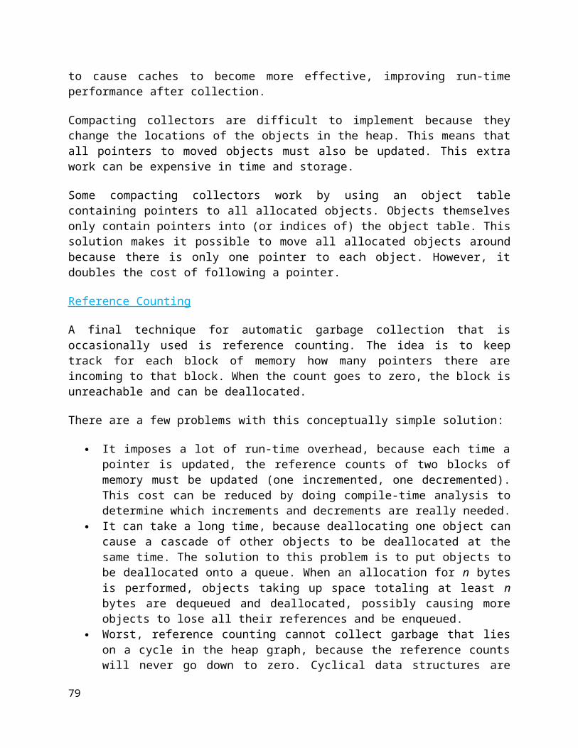
break; case 6:

display(root,1);break;

case 7:exit();

default:printf("Wrong choice\n");

}}

}Questions

Objective What is BST?

Long Answer type- Explain the different methods of binary search tree traversal.With the sequence of input-10,8,20,5,3. Construct a BST.

79

Lecture-28B+ tree

B - Tree 

Tree structures support various basic dynamic set operations including Search , Insert , and Delete in time proportional to the height of the tree. Ideally, a tree will be balanced and the height will be log n where n is the number of nodes in the tree. To ensure that the height of the tree is as small as possible and therefore provide the best running time, a balanced tree structure like AVL tree , 2-3 Tree , Red Black Tree or B-tree must be used.

When working with large sets of data, it is often not possible or desirable to maintain the entire structure in primary storage (RAM). Instead, a relatively small portion of the data structure is maintained in primary storage, and additional data is read from secondary storage as needed. Unfortunately, a magnetic disk, the most common form of secondary storage, is significantly slower than random access memory (RAM). In fact, the system often spends more time retrieving data than actually processing data.

To reduce the time lost in retrieving data from secondary storage, we need to minimize the no. of references to the secondary memory. This is possible if a node in a tree contains more no. of values, then in a single reference to the secondary memory more nodes can be accessed. The AVL trees or red Black Trees can hold a max. of 1 value only in a node while 2-3 Trees can hold a max of 2 values per node. To improve the efficiency Multiway Search Trees are used.

Multiway Search Trees    

A Multiway Search Tree of order n is a tree in which any node can have a maximum of n-1 values & a max. of n children. B - Trees are a special case of Multiway Search Trees.

A B Tree of order n is a Multiway Search Tree of order n with the following characteristics:

A. All the non leaf nodes have a max of n child nodes & a min of n/2 child nodes. B. If a root is non leaf node, then it has a max of n non empty child nodes & a min of 2 child

nodes. C. If a root node is a leaf node, then it does not have any child node. D. A node with n child nodes has n-1 values arranged in ascending order. E. All values appearing on the left most child of any node are smaller than the left most

value of that node while all values appearing on the right most child of any node are greater than the right most value of that node.

F. If x & y are two adjacent values in a node such that x < y, ie they are the i th & (i+1) th values in the node respectively, then all values in the (i+1) th child of that node are > x but < y.

80

REPRESENTATION OF B - TREE The B - Tree is represented as follows using structure:

        Struct btnode       {           int count;           int value[max+1];           Struct btnode * child[max + 1];       };

Count is the no. of children of any node. The values of node are in the array value. The addresses of child nodes are in child array while the Max is a macro that defines the maximum no. of values any node can have.

THE following operations can be done on a B - Tree :

1. Searching 2. Insertion 3. Deletion

When we try to insert the H, we find no room in this node, so we split it into 2 nodes, moving the median item G up into a new root node. Note that in practice we just leave the A and C in the current node and place the H and N into a new node to the right of the old one.

81

      Inserting E, K, and Q proceeds without requiring any splits:    

Inserting M requires a split. Note that M happens to be the median key and so is moved up into the parent

82

DELETION IN A B - TREE     Deletion in a B -Tree is similar to insertion.At first the node from which a value is to be deleted is searched.If found out, then the value is deleted. After deletion the tree is checked if it still follows B - Tree properties. Let us take an example.THe original B - Tree taken is as follows:    

         

Delete H. first it is found out.Since H is in a leaf and the leaf has more than the minimum number of keys, this is easy. We move the K over where the H had been and the L over where the K had been. This gives:

Next, delete the T. Since T is not in a leaf, we find its successor (the next item in ascending order), which happens to be W, and move W up to replace the T. That way, what we really have to do is to delete W from the leaf, which we already know how to do, since this leaf has extra keys. In ALL cases we reduce deletion to a deletion in a leaf, by using this method

83

             Next, delete R. Although R is in a leaf, this leaf does not have an extra key; the deletion results in a node with only one key, which is not acceptable for a B-tree of order 5. If the sibling node to the immediate left or right has an extra key, we can then borrow a key from the parent and move a key up from this sibling. In our specific case, the sibling to the right has an extra key. So, the successor W of S (the last key in the node where the deletion occurred), is moved down from the parent, and the X is moved up. (Of course, the S is moved over so that the W can be inserted in its proper place.)

     

Finally, let's delete E. This one causes lots of problems. Although E is in a leaf, the leaf has no extra keys, nor do the siblings to the immediate right or left. In such a case the leaf has to be combined with one of these two siblings. This includes moving down the parent's key that was between those of these two leaves. In our example, let's combine the leaf containing F with the leaf containing A C. We also move down the D.

84

                Questions

Objective What is b+ tree give one example.

Long Answer type- Write short notes on B-tree and B+tree.

85

Lecture-29AVL Tree

INTRODUCTION   As we know that searching in a binary search tree is efficient if the height of the left sub-tree and right sub-tree is same for a node. But frequent insertion and deletion in the tree affects the efficiency and makes a binary search tree inefficient. The efficiency of searching will be ideal if the difference in height of left and right sub-tree with respect of a node is at most one. Such a binary search tree is called balanced binary tree (sometimes called AVL Tree).

REPRESENTATION OF AVL TREE

In order to represent a node of an AVL Tree, we need four fields :- One for data, two for storing address of left and right child and one is required to hold the balance factor. The balance factor is calculated by subtracting the right sub-tree from the height of left sub - tree.

The structure of AVL Tree can be represented by : - Struct AVL          {              struct AVL *left;               int data;               struct AVL *right;               int balfact;           };

DETERMINATION OF BALANCE FACTOR

The value of balance factor may be -1, 0 or 1. Any value other than these represent that the tree is not an AVL Tree

1. If the value of balance factor is -1, it shows that the height of right sub-tree is one more than the height of the left sub-tree with respect to the given node.

2. If the value of balance factor is 0, it shows that the height of right sub-tree is equal to the height of the left Sub-tree with respect to the given node.

3. If the value of balance factor is 1, it shows that the height of right sub-tree is one less than the height of the left sub-tree with respect to the given node .

86

Types of rotation-o LL rotation,RR rotation,LR rotation,RL rotation

Operations on AVL tree. Insertion,deletion

INSERTION OF A NODE IN AVL TREE              

Insertion can be done by finding an appropriate place for the node to be inserted. But this can disturb the balance of the tree if the difference of height of sub-trees with respect to a node exceeds the value one. If the insertion is done as a child of non-leaf node then it will not affect the balance, as the height doesn't increase. But if the insertion is done as a child of leaf node, then it can bring the real disturbance in the balance of the tree.

This depends on whether the node is inserted to the left sub-tree or the right sub-tree, which in turn changes the balance factor. If the node to be inserted is inserted as a node of a sub-tree of smaller height then there will be no effect. If the height of both the left and right sub-tree is same then insertionto any of them doesn't affect the balance of AVL Tree. But if it is inserted as a node of sub-tree of larger height, then the balance will be disturbed.

To rebalance the tree, the nodes need to be properly adjusted. So, after insertion of a new node the tree is traversed starting from the new node to the node where the balance has been disturbed. The nodes are adjusted in such a way that the balance is regained.

ALGORITHM FOR INSERTION IN AVL TREE   int avl_insert(node *treep, value_t target)           { /* insert the target into the tree, returning 1 on success or 0 if it * already existed */

87

          node tree = *treep;           node *path_top = treep;                 while (tree && target != tree->value)                     {                         direction next_step = (target > tree->value);                         if (!Balanced(tree)) path_top = treep;                         treep = &tree->next[next_step];                         tree = *treep;                     }                 if (tree) return 0;                     tree = malloc(sizeof(*tree));                     tree->next[0] = tree->next[1] = NULL;                     tree->longer = NEITHER;                     tree->value = target;                     *treep = tree;                     avl_rebalance(path_top, target);       return 1;           }

ALGORITHM FOR REBALANCING IN INSERTION

  void avl_rebalance_path(node path, value_t target)                {/* Each node in path is currently balanced. Until we find target, mark each node as longer in the direction of rget because we know we have inserted target there */                        while (path && target != path->value) {                        direction next_step = (target > path->value);                        path->longer = next_step;                        path = path->next[next_step];                     }               }  void avl_rebalance(node *path_top, value_t target)                {                    node path = *path_top;                    direction first, second, third;                    if (Balanced(path)) {                    avl_rebalance_path(path, target);                    return;                 }         first = (target > path->value);                 if (path->longer != first) {

88

                   /* took the shorter path */                    path->longer = NEITHER;                    avl_rebalance_path(path->next[first], target);                    return;                 }/* took the longer path, need to rotate */ second = (target > path->next[first]->value);          if (first == second) { /* just a two-point rotate */                path = avl_rotate_2(path_top, first);                avl_rebalance_path(path, target);                return;                }/* fine details of the 3 point rotate depend on the third step. However there may not be a third step, if the third point of the rotation is the newly inserted point. In that case we record the third step as NEITHER */ path = path->next[first]->next[second];        if (target == path->value) third = NEITHER;                else third = (target > path->value);                         path = avl_rotate_3(path_top, first, third);                         avl_rebalance_path(path, target);                }

89

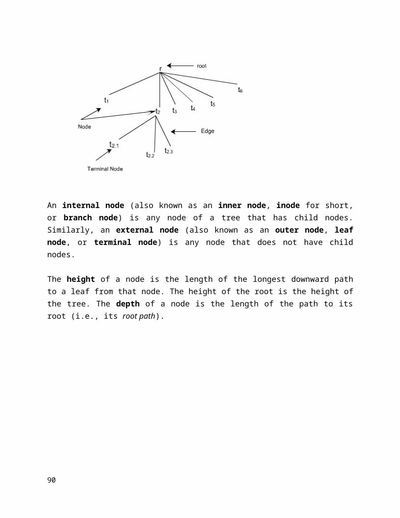
DELETION

A node in AVL Tree is deleted as it is deleted in the binary search tree. The only difference is that we have to do rebalancing which is done similar to that of insertion of a node in AVL Tree.The algorithm for deletion and rebalancing is given below:

REBALANCING OF AVL TREE When we insert a node to the taller sub-tree, four cases arise and we have different rebalancing methods to bring it back to a balanced tree form.

1. Left Rotation 2. Right Rotation 3. Right and Left Rotation 4. Left and Right Rotation

90

                          Before Rotation

After Rotation   EXPLANATION OF EXAMPLE  

In the given AVL tree when we insert a node 8,it becomes the left child of node 9 and the balance doesn't exist, as the balance factor of node 3 becomes -2. So, we try to rebalance it. In order to do so, we do left rotation at node 3. Now node 5 becomes the left child of the root. Node 9 and node 3 becomes the right and left child of node 5 respectively. Node 2 and node 4 becomes the left and right child of node 3 respectively. Lastly, node 8 becomes the left child of node 9. Hence, the balance is once again attained and we get AVL Tree after the left rotation.

RIGHT ROTATION

In general if we want to insert a node R(either as left or right child) to N1 as shown in figure. Here, as we see the balance factor of node P becomes 2. So to rebalance it, we have a technique called right rotation.

91

  EXAMPLE GENERAL DIAGRAM

Before Rotation After Rotation

EXPLANATION OF EXAMPLE

In the given AVL tree when we insert a node 7,it becomes the right child of node 5 and the balance doesn't exist, as the balance factor of node 20 becomes 2. So, we try to rebalance it. In order to do so, we do right rotation at node 20. Now node 10 becomes the root. Node 12 and node 7 becomes the right and left child of root respectively. Node 20 becomes the right child of

92

node 12. Node 30 becomes the right child of node 20. Lastly, node 5 becomes the left child of node 7. Hence, the balance is once again attained and we get AVL Tree after the right rotation RIGHT AND LEFT ROTATION   In general if we want to insert a node R(either as a left or right child)to N2 as shown in figure. Here, as we see the balance factor of node P becomes -2. So to rebalance it, we have to do two rotations. Firstly, right rotation and then left rotation.

Questions Objective

What is height balance Tree? What is balance factor?What are the types of rotation?

Long Answer type- Insert node in an AVL tree- 55,66,77,15,11,33,22,35,25,44

93

Lecture-30Complete Binary Tree representation

What is Complete Binary Tree?In a complete binary tree every level, except possibly the last, is completely filled, and all nodes are as far left as possible. It can have between 1 and 2h nodes, as far left as possible, at the last level h.[20] A binary tree is called an almost complete binary tree or nearly complete binary tree if mentioned exception holds, i.e. the last level is not completely filled. This type of binary tree is used as a specialized data structure called a Binary heap.

Questions Objective

What is Complete Binary Tree? Long Answer type-

What is heap tree? Discuss Heap tree with suitable example.Create a heap from the following sequence of integer-50,40,60,80,70,20,90,10,8,2,5,100.

94

Lecture-31 &32Tree traversals

Traversal of a binary tree means to visit each node in the tree exactly once. The tree traversal is used in all the applications of it.

In a linear list nodes are visited from first to last, but a tree being a non linear one we need definite rules. There are a no. of ways to traverse a tree. All of them differ only in the order in which they visit the nodes.

The three main methods of traversing a tree are:

Inorder Traversal Preorder Traversal Postorder Traversal

In all of them we do not require to do anything to traverse an empty tree. All the traversal methods are based on recursive functions since a binary tree is itself recursive as every child of a node in a binary tree is itself a binary tree.

To traverse a non empty tree in inorder the following steps are followed recursively.

Visit the Root Traverse the left subtree Traverse the right subtree

The inorder traversal of the tree shown below is as follows.

95

Inorder Traversal :

Algorithm The algorithm for inorder traversal is as follows.

Struct node{ struct node * lc; int data; struct node * rc; };

void inorder(struct node * root); { if(root != NULL) { inorder(roo-> lc); printf("%d\t",root->data); inorder(root->rc); } }

So the function calls itself recursively and carries on the traversal.

What is traversing? Types of traversing

Preorder, Inorder, Postorder. Algorithm to traverse a binary tree. Tree construction.

Questions Objective

96

What are the way to traverse a tree?

Long Answer type question-o Draw the BST from the key-39,24,12,11,43,73. Write the pre-order traversal of the same.o The in-order traversal of a tree produced the sequence D,B,H,E,A,I,F,J,C,G and the

preorder traversal of the same tree produced A,B,D,E,H,C,F,I,J,G .Draw the binary tree.Give a linear array representation of the above binary tree.Define a node structure in C,which can be used to implement a tree.

o Write a program to create a BT and traverse it.

97

Lect-33 Operation on Binary tree-Expression manipulation

Infix

Infix is the one we are all most familiar with. In this notation, all binary operators appear between the two operands. This provides several advantages to the other two notations- mainly, it is easy to see which operators are bound to which operands. At a glance (at least in my opinion) it is also easier to solve these equations mentally. Infix does create a few problems, however. Because operators appear where they do, when they are stacked and equations become more complex, it's hard to distinguish one operand from another. The solution is to use parentheses to group operations. Infix appears as:

((1+2) * (3-4))

Prefix

This type of notation is arguably the easiest to use. In prefix, all operators appear near the beginning of the equation, with the two operands appearing right after. When operations are stacked, it becomes difficult to see how these operands are grouped, but because of the nature of prefix notation, no parentheses are needed to group them. To stop nodes (the operands) from running together, spaces are added between each one of them. Prefix appears as:

* + 1 2 - 3 4

98

Evaluate Postfix Expression• Evaluate: 23+8*• Push the operands, 2, 3 until you get an operator.• When you get the operator +, pop the two topmost elements and apply the operator on them. Then push the result, 5 into the stack. Continue Pushing 8. Then apply * to 8 and 5 (after popping them). Thus, the expression evaluates to 40.

Expression Trees• Expression Trees are binary trees and compact representations of expressions• We shall discuss a technique to convert postfix expressions to trees.

Method: – If the symbol is an operand, create a one-node tree and push its pointer to a stack.– If the symbol is an operator, we pop twice to obtain pointers T1 and T2 to two trees.– If T1 is first popped, then form a tree with the operator as root. The left child points to T2 and right to T1.Then push the new pointer to the stack.

99

Traversing the expression treePostorder Traversal• abc*+de*f+g*+(gives back the postfix expression)

Evaluate the expression tree

Use Recursion1. If the root is an operand, return value.2. Else evaluate the left tree.3. Evaluate the right tree.4. Apply the operator on the two returned results.5. Return the result.

100

A possible representation• #define OPERATOR 0• #define OPERAND 1• struct nodetype{shortint utype;union{char chinfo;float numinfo;}info;struct nodetype *left;struct nodetype *right;};typedef struct nodetype *NODEPTR;

101

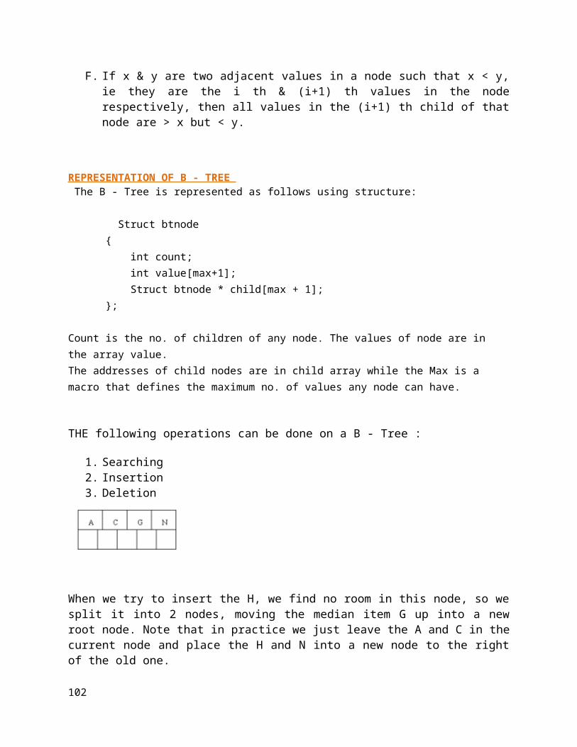
Lect. 35GRAPH

A graph consists of a set of nodes (or Vertices) and a set of arc (or edge). Each arc in a graph is specified by a pair of nodes. A node n is incident to an arc x if n is one of the two nodes in the ordered pair of nodes that constitute x. The degree of a node is the number of arcs incident to it. The indegree of a node n is the number of arcs that have n as the head, and the outdegree of n is the number of arcs that have n as the tail.

The graph is the nonlinear data structure. The graph shown in the figure represents 7 vertices and 12 edges. The Vertices are { 1, 2, 3, 4, 5, 6, 7} and the arcs are {(1,2), (1,3), (1,4), (2,4), (2,5), (3,4), (3,6), (4,5), (4,6), (4,7), (5,7), (6,7) }. Node (4) in figure has indegree 3, outdegree 3 and degree 6.              

Graph consists of a non empty set of points called vertices and a set of edges that link vertices.

Formal Definition :

Definition: A graph G= (V, E) consists of

a set V={v1 , v2 .....,vn } of n >1 vertices and a set of E={e1 ,e2 ,.....,em } of m>0 edges such that each edge ek is corresponds to an un ordered pair of vertices (vi ,vj) where 0 < i,j <= n and 0 < k <= m.

102

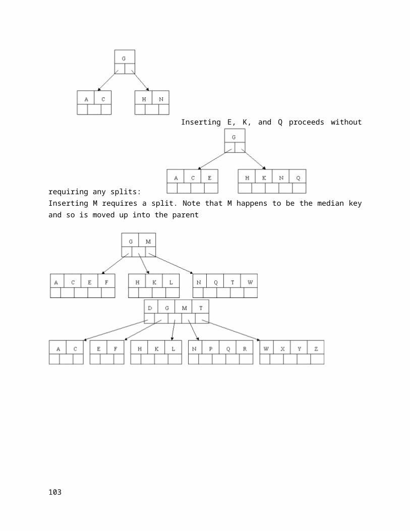
Example-

A road network is simple examples of a graph, in which vertices reprents cities and road connecting them are correspond to edges.

V= { Delhi, Chenai, Kolkata, Mumbai, Nagpur } E= { (Delhi, Kolkata), (Delhi, Mumbai}, (Delhi, Nagpur), (Chenai, Kolkata), (Chenai, Mumbai), (Chenai, Nagpur), (Kolkata, Nagpur), (Mumbai, Nagpur) }

Graph Terminology

A Graph without loops and parallel edges is called a simple graph. A graph with isolated vertices (no edges) is called null graph. Set of edges E can be empty for a graph but not set of vertices V. Incidence: if an vertex vi is an end vertex of an edge ek , we say vertex vi is incident on

ek and ek is incident on vi.   e1 is incident on v1 and v3 in the below figure.

v4 is incidnet on e3 , e4 , and e5 in the figure below. Degree: Degree of an vertex is number of edges incident on it, with loops counted twice.

      d(v1 ) = 2, d(v2 ) = 4, d(v3 ) = 3, and d(v4 ) = 3 in the figure below.

    

Adjacent Edges: Two non parallel edges are adjacent if they have a vertex in common. e1 and e2 , e2 and e6 , e2 and e3 , e1 and e4 are adjacent edges in the above diagram.

Adjacent vertices: Two vertices are adjacent if they are connected by an edge.   v1 and v3 , v1 and v2 , v2 and v4 are adjacent vertices in the above diagram.        

An isolated vertex is a vertex with degree zero; that is, a vertex that is not an endpoint of any edge.

A leaf vertex (also pendant vertex) is a vertex with degree one. A source vertex is a vertex with in degree zero, while a sink vertex is a vertex with out

degree zero.

103

Lect.36GRAPHS Representation :

         

Graph Representation: There are several different ways to represent graphs in a computer. Two main representaions are Adjacency Matrix and Adjacency list.

Adjacency Matrix Representation:      An adjacency matrix of a graph G=(V,E) (let V = { v 1 , v 2 ....., v n}) is a n X n matrix A, such that

A [i, j] = 1      if there is edge between vi and v j.

0     other wise    

I.

Adjacency List Representation:

It consists of a list of vertices, which can be represented either by linked list or array. For each vertex, adjacent vertices are represented in the form of a linked list.

An example is given below.

Size of the adjacency lists is proposnal to number of edges and vertices. It is an efficient memory use for sparse graphs. Accessing an element takes linear time, since it involves traversal of linked list.

104

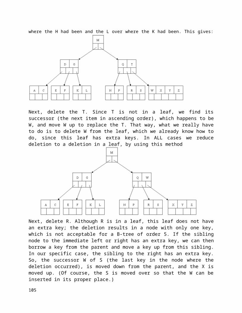
Lect.37 Graph Traversals

Many graph problems can be solved by visiting each and every vertex in a systamatic manner.

There are two main method to traversal graphs,

1. Depth First Search (DFS)

2. Breadth First Search (BFS).

Breadth First Search (BFS).

In graph theory, breadth-first search (BFS) is a strategy for searching in a graph when search is limited to essentially two operations: (a) visit and inspect a node of a graph; (b) gain access to visit the nodes that neighbor the currently visited node. The BFS begins at a root node and inspects all the neighboring nodes. Then for each of those neighbor nodes in turn, it inspects their neighbor nodes which were unvisited, and so on. Compare BFS with the equivalent, but more memory-efficient Iterative deepening depth-first search and contrast with depth-first search.

Input: A graph G and a root v of G

1 procedure BFS(G,v) is2 create a queue Q3 create a set V4 add v to V5 enqueue v onto Q6 while Q is not empty loop7 t ← Q.dequeue()8 if t is what we are looking for then9 return t10 end if11 for all edges e in G.adjacentEdges(t) loop12 u ← G.adjacentVertex(t,e)13 if u is not in V then14 add u to V15 enqueue u onto Q16 end if17 end loop18 end loop19 return none20 end BFS

105

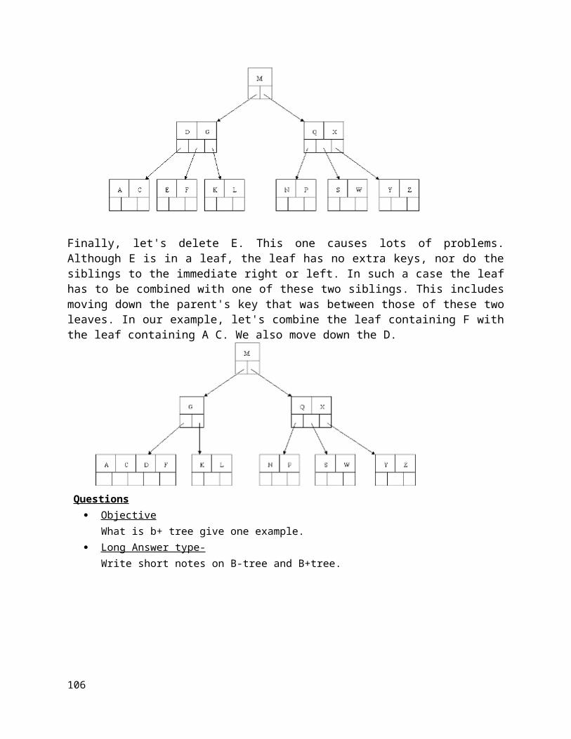
Path Matrix

The path matrix denoted by P, the P-matrix of a vertex-labeled connected simple graph G is a square V x V matrix whose entries are defined as follows:

[P]ij=

p'(i,j)/p if i ≠ j

0 otherwise

The concept of path matrix of G if G is a simple directed graph. A graph consists of a set of nodes which are also known as vertices and a set of arcs also known as edges. Each graph is specified by a pair of nodes. If the pairs of nodes that make up the arcs are ordered pairs, the graph is said to be a directed graph. A directed graph, or "digraph", is a graph whose arcs have direction. Arrows on the arcs are used to show the directional information. An arc from node A to node B indicates that one may move from A to B but not from B to A. This is most commonly known as the simple directed graph.

In a simple directed graph to show adjacent nodes we use the concept of adjacency matrix. Adjacency matrix is a matrix stored in the form of a two dimensional array in memory that represents every possible ordered pair of nodes in a simple directed graph. The graph could be totally described by its adjacency matrix. The adjacency matrix is filled with Boolean values 0 and 1. If for example a graph exists with two nodes A and B and the direction is denoted by an arrow from A B then the value <A,B> = 1 but <B,A>= 0 like wise by doing so for all the nodes in the graph we create the adjacency matrix. For example consider the following simple directed graph G.

106

Above shown is the adjacency matrix for the simple directed graph G portrayed above. Here from the above matrix what we can mainly describe is the relationships between the adjacent nodes. However we are able to see that other relationships also exist. In the above if we consider the three nodes B, C and E we see that <B, C> = 1 and also <C, E> = 1 hence it is understood that there is a link directed from B to E through C. Thus in order to show such relationship we use the concept of path matrix. Just like its name describes it represents paths of certain length. In the above case when we consider nodes B, C and E only two arcs were used hence we say that it is a path of length 2. And furthermore if we consider all such paths of length 2 we could represent them using a path matrix of length 2. It is as shown below.

The path matrix of length 2 can be easily obtained by getting the Boolean product of the adjacent matrix with itself. We could move on further and consider all paths of length 3 in the above graph. Thus the following could be obtained.

Above matrix is known as a path matrix of length 3. Therefore we could define path matrices of certain lengths to show paths among nodes in a graph if they exist. Furthermore by getting the OR of the adjacency matrix and all the path matrices we could obtain the matrix path.

107

Lect.38 Depth First Search (DFS)

This method is called depth first search since searching is done forward (deeper) from current node. The distance from start vertex is called depth.

Deapth First Search (DFS): Initially all vertices of the graph are unvisited. Start visiting the graph from any vertex, say v. For each unvisited adjacent vertex of v, search recursively. This process stops when all vertices reachable from v are visited. If there are any more unvisited vertices are present select any unvisited vertex and repeat the same search process.

Depth-first search (DFS) is an algorithm for traversing or searching tree or graph data structures. One starts at the root (selecting some arbitrary node as the root in the case of a graph) and explores as far as possible along each branch before backtracking.

Input: A graph G and a vertex v of G

Output: All vertices reachable from v labeled as discovered

A recursive implementation of DFS:

1 procedure DFS(G,v):2 label v as discovered3 for all edges from v to w in G.adjacentEdges(v) do4 if vertex w is not labeled as discovered then5 recursively call DFS(G,w)

A non-recursive implementation of DFS:

1 procedure DFS-iterative(G,v):2 let S be a stack3 S.push(v)4 while S is not empty5 v ← S.pop() 6 if v is not labeled as discovered:7 label v as discovered8 for all edges from v to w in G.adjacentEdges(v) do9 S.push(w)

108

Lect. 39 Topological sort

In computer science, a topological sort (sometimes abbreviated topsort or toposort) or topological ordering of a directed graph is a linear ordering of its vertices such that for every directed edge uv from vertex u to vertex v, u comes before v in the ordering. For instance, the vertices of the graph may represent tasks to be performed, and the edges may represent constraints that one task must be performed before another; in this application, a topological ordering is just a valid sequence for the tasks. A topological ordering is possible if and only if the graph has no directed cycles, that is, if it is a directed acyclic graph (DAG). Any DAG has at least one topological ordering, and algorithms are known for constructing a topological ordering of any DAG in linear time.

The canonical application of topological sorting (topological order) is in scheduling a sequence of jobs or tasks based on their dependencies; topological sorting algorithms were first studied in the early 1960s in the context of the PERT technique for scheduling in project management (Jarnagin 1960). The jobs are represented by vertices, and there is an edge from x to y if job x must be completed before job y can be started (for example, when washing clothes, the washing machine must finish before we put the clothes to dry). Then, a topological sort gives an order in which to perform the jobs.

In computer science, applications of this type arise in instruction scheduling, ordering of formula cell evaluation when recomputing formula values in spreadsheets, logic synthesis, determining the order of compilation tasks to perform in makefiles, data serialization, and resolving symbol dependencies in linkers. It is also used to decide in which order to load tables with foreign keys in databases.

The graph shown to the left has many valid topological sorts, including:

7, 5, 3, 11, 8, 2, 9, 10 (visual left-to-right, top-to-bottom) 3, 5, 7, 8, 11, 2, 9, 10 (smallest-numbered available vertex

first) 5, 7, 3, 8, 11, 10, 9, 2 (fewest edges first) 7, 5, 11, 3, 10, 8, 9, 2 (largest-numbered available vertex

first) 7, 5, 11, 2, 3, 8, 9, 10 (attempting top-to-bottom, left-to-right) 3, 7, 8, 5, 11, 10, 2, 9 (arbitrary)

Algorithm

L ← Empty list that will contain the sorted elementsS ← Set of all nodes with no incoming edgeswhile S is non-empty do remove a node n from S

109

add n to tail of L for each node m with an edge e from n to m do remove edge e from the graph if m has no other incoming edges then insert m into Sif graph has edges then return error (graph has at least one cycle)else return L (a topologically sorted order)

110

Lect.40 Floyd–Warshall algorithm

In computer science, the Floyd–Warshall algorithm (also known as Floyd's algorithm, Roy–Warshall algorithm, Roy–Floyd algorithm, or the WFI algorithm) is a graph analysis algorithm for finding shortest paths in a weighted graph with positive or negative edge weights (but with no negative cycles, see below) and also for finding transitive closure of a relation . A single execution of the algorithm will find the lengths (summed weights) of the shortest paths between all pairs of vertices, though it does not return details of the paths themselves.

The Floyd–Warshall algorithm compares all possible paths through the graph between each pair of vertices. It is able to do this with Θ(|V |3) comparisons in a graph. This is remarkable considering that there may be up to Ω(|V |2) edges in the graph, and every combination of edges is tested. It does so by incrementally improving an estimate on the shortest path between two vertices, until the estimate is optimal.

Consider a graph G with vertices V numbered 1 through N. Further consider a function shortestPath(i, j, k) that returns the shortest possible path from i to j using vertices only from the set {1,2,...,k} as intermediate points along the way. Now, given this function, our goal is to find the shortest path from each i to each j using only vertices 1 to k + 1.

For each of these pairs of vertices, the true shortest path could be either (1) a path that only uses vertices in the set {1, ..., k} or (2) a path that goes from i to k + 1 and then from k + 1 to j. We know that the best path from i to j that only uses vertices 1 through k is defined by shortestPath(i, j, k), and it is clear that if there were a better path from i to k + 1 to j, then the length of this path would be the concatenation of the shortest path from i to k + 1 (using vertices in {1, ..., k}) and the shortest path from k + 1 to j (also using vertices in {1, ..., k}).

If is the weight of the edge between vertices i and j, we can define shortestPath(i, j, k + 1) in terms of the following recursive formula: the base case is

and the recursive case is

This formula is the heart of the Floyd–Warshall algorithm. The algorithm works by first computing shortestPath(i, j, k) for all (i, j) pairs for k = 1, then k = 2, etc. This process continues until k = n, and we have found the shortest path for all (i, j) pairs using any intermediate vertices. Pseudocode for this basic version follows:

1 let dist be a |V| × |V| array of minimum distances initialized to ∞ (infinity)2 for each vertex v3 dist[v][v] ← 04 for each edge (u,v)

111

5 dist[u][v] ← w(u,v) // the weight of the edge (u,v)6 for k from 1 to |V|7 for i from 1 to |V|8 for j from 1 to |V|9 if dist[i][j] > dist[i][k] + dist[k][j] 10 dist[i][j] ← dist[i][k] + dist[k][j]11 end if

Prior to the first iteration of the outer loop, labeled k=0 above, the only known paths correspond to the single edges in the graph. At k=1, paths that go through the vertex 1 are found: in particular, the path 2→1→3 is found, replacing the path 2→3 which has fewer edges but is longer. At k=2, paths going through the vertices {1,2} are found. The red and blue boxes show how the path 4→2→1→3 is assembled from the two known paths 4→2 and 2→1→3 encountered in previous iterations, with 2 in the intersection. The path 4→2→3 is not considered, because 2→1→3 is the shortest path encountered so far from 2 to 3. At k=3, paths going through the vertices {1,2,3} are found. Finally, at k=4, all shortest paths are found.

Algorithm Dijkstra_shortest_path (G, v_0)

Step 1: for each vertex vi in V do Step 2:     dist[vi} = infinity Step 3: distance[v0] = 0;

112

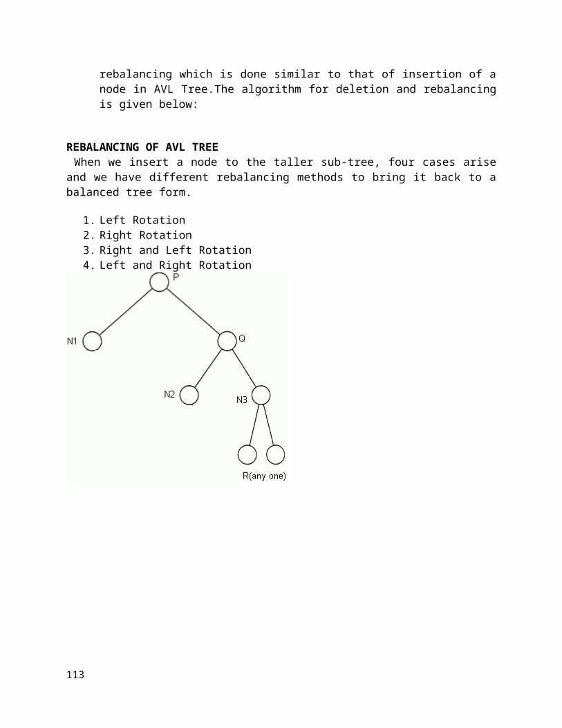
Step 4:     for each vertex v_i in V do Step 5:         insert(Q, vi)Step 6: S = emptyStep 7: while (Q not empty) doStep 8:         vi = Min(Q) Step 9:         for each vertex vj adjacent to vi do Step 10:       distance[vj] = Minimum (distance[vj], distance[vi] + w[vi,vj])

Consider the following graph:

     

113

Lecture-41 Sorting

Bubble sort

Bubble sort, sometimes referred to as sinking sort, is a simple sorting algorithm that works by repeatedly stepping through the list to be sorted, comparing each pair of adjacent items and swapping them if they are in the wrong order. The pass through the list is repeated until no swaps are needed, which indicates that the list is sorted. The algorithm gets its name from the way smaller elements "bubble" to the top of the list. Because it only uses comparisons to operate on elements, it is a comparison sort. Although the algorithm is simple, it is too slow for practical use, even compared to insertion sort.

Step-by-step example

Let us take the array of numbers "5 1 4 2 8", and sort the array from lowest number to greatest number using bubble sort. In each step, elements written in bold are being compared. Three passes will be required.

First Pass:

( 5 1 4 2 8 ) ( 1 5 4 2 8 ), Here, algorithm compares the first two elements, and swaps since 5 > 1.( 1 5 4 2 8 ) ( 1 4 5 2 8 ), Swap since 5 > 4( 1 4 5 2 8 ) ( 1 4 2 5 8 ), Swap since 5 > 2( 1 4 2 5 8 ) ( 1 4 2 5 8 ), Now, since these elements are already in order (8 > 5), algorithm does not swap them.Second Pass:( 1 4 2 5 8 ) ( 1 4 2 5 8 )( 1 4 2 5 8 ) ( 1 2 4 5 8 ), Swap since 4 > 2( 1 2 4 5 8 ) ( 1 2 4 5 8 )( 1 2 4 5 8 ) ( 1 2 4 5 8 )Now, the array is already sorted, but our algorithm does not know if it is completed. The algorithm needs one whole pass without any swap to know it is sorted.Third Pass:( 1 2 4 5 8 ) ( 1 2 4 5 8 )( 1 2 4 5 8 ) ( 1 2 4 5 8 )( 1 2 4 5 8 ) ( 1 2 4 5 8 )( 1 2 4 5 8 ) ( 1 2 4 5 8 )

The algorithm can be expressed as (0-based array):

procedure bubbleSort( A : list of sortable items ) n = length(A) repeat

114

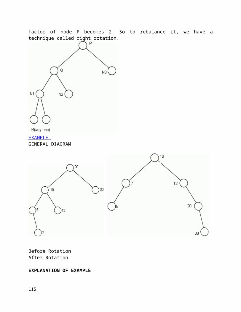
swapped = false for i = 1 to n-1 inclusive do /* if this pair is out of order */ if A[i-1] > A[i] then /* swap them and remember something changed */ swap( A[i-1], A[i] ) swapped = true end if end for until not swappedend procedure

115

Lecture-42 Insertion sort

Insertion sort is a simple sorting algorithm that builds the final sorted array (or list) one item at a time. It is much less efficient on large lists than more advanced algorithms such as quicksort, heapsort, or merge sort. However, insertion sort provides several advantages:

Simple implementation: Bentley shows a three-line C version, and a five-line optimized version[1]:116

Efficient for (quite) small data sets More efficient in practice than most other simple quadratic (i.e., O(n2)) algorithms such as

selection sort or bubble sort Adaptive, i.e., efficient for data sets that are already substantially sorted: the time complexity is

O(nk) when each element in the input is no more than k places away from its sorted position Stable; i.e., does not change the relative order of elements with equal keys In-place; i.e., only requires a constant amount O(1) of additional memory space Online; i.e., can sort a list as it receives it

Example: The following table shows the steps for sorting the sequence {3, 7, 4, 9, 5, 2, 6, 1}. In each step, the key under consideration is underlined. The key that was moved (or left in place because it was biggest yet considered) in the previous step is shown in bold.

o 3 7 4 9 5 2 6 1o 3 7 4 9 5 2 6 1o 3 7 4 9 5 2 6 1o 3 4 7 9 5 2 6 1o 3 4 7 9 5 2 6 1o 3 4 5 7 9 2 6 1o 2 3 4 5 7 9 6 1o 2 3 4 5 6 7 9 1o 1 2 3 4 5 6 7 9

Selection Sort

In computer science, selection sort is a sorting algorithm, specifically an in-place comparison sort. It has O(n2) time complexity, making it inefficient on large lists, and generally performs worse than the similar insertion sort. Selection sort is noted for its simplicity, and it has performance advantages over more complicated algorithms in certain situations, particularly where auxiliary memory is limited.

The algorithm divides the input list into two parts: the sublist of items already sorted, which is built up from left to right at the front (left) of the list, and the sublist of items remaining to be sorted that occupy the rest of the list. Initially, the sorted sublist is empty and the unsorted sublist is the entire input list. The algorithm proceeds by finding the smallest (or largest, depending on sorting order) element in the unsorted sublist, exchanging it with the leftmost unsorted element (putting it in sorted order), and moving the sublist boundaries one element to the right.

116

Here is an example of this sort algorithm sorting five elements:

64 25 12 22 11 // this is the initial, starting state of the array

11 25 12 22 64 // sorted sublist = {11}

11 12 25 22 64 // sorted sublist = {11, 12}

11 12 22 25 64 // sorted sublist = {11, 12, 22}

11 12 22 25 64 // sorted sublist = {11, 12, 22, 25}

11 12 22 25 64 // sorted sublist = {11, 12, 22, 25, 64}

117

Lecture-43 QUICK SORT

Quicksort, or partition-exchange sort, is a sorting algorithm developed by Tony Hoare that, on average, makes O(n log n) comparisons to sort n items. In the worst case, it makes O(n2) comparisons, though this behavior is rare. Quicksort is often faster in practice than other O(n log n) algorithms. Additionally, quicksort's sequential and localized memory references work well with a cache. Quicksort is a comparison sort and, in efficient implementations, is not a stable sort. Quicksort can be implemented with an in-place partitioning algorithm, so the entire sort can be done with only O(log n) additional space used by the stack during the recursion.

#include <stdio.h>#define MAX 500void quickSort(int A[], int maxsize);void sort(int A[], int left, int right);int A[MAX];

void main(){int i, max;clrscr();printf("\nHow many elements you want to sort: ");scanf("%d",&max);printf("\nEnter the values one by one: ");

for (i = 0; i < max; i++)scanf("%d",&A[i]);

printf("\nArray before sorting:");for (i= 0;i< max;i++)printf("%d",A[i]);

printf ("\n");

quickSort(A, max);

printf("\nArray after sorting:");for (i = 0; i < max; i++)printf("%d ", A[i]);getch();}

118

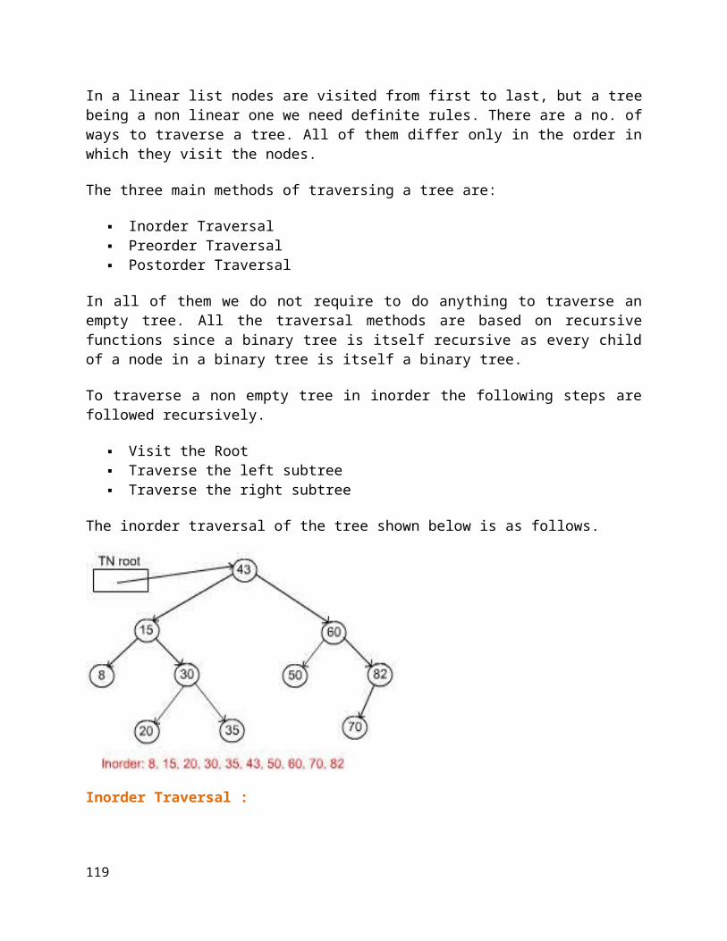
void quickSort(int A[], int max){sort(A,0,max - 1);}

void sort(int A[], int left, int right){int pivot, l, r;l = left;r = right;pivot = A[left];while (left < right){

while ((A[right] >= pivot) && (left < right))right--;if (left != right){

A[left] = A[right];left++;

}while ((A[left] <= pivot) && (left < right))left++;if(left != right){

A[right] = A[left];right--;

}}A[left] = pivot;pivot = left;left = l;right = r;

if (left < pivot)sort(A, left, pivot - 1);if (right > pivot)sort(A, pivot + 1, right);}

119

MERGE SORT

In computer science, merge sort (also commonly spelled mergesort) is an O(n log n) comparison-based sorting algorithm. Most implementations produce a stable sort, which means that the implementation preserves the input order of equal elements in the sorted output. Mergesort is a divide and conquer algorithm that was invented by John von Neumann in 1945.

#include<stdio.h>#define MAX 50void mergeSort(int arr[],int low,int mid,int high); void partition(int arr[],int low,int high);void main(){ int merge[MAX],i,n; printf("Enter the total number of elements: "); scanf("%d",&n); printf("Enter the elements which to be sort: "); for(i=0;i<n;i++)

scanf("%d",&merge[i]);

partition(merge,0,n-1); printf("After merge sorting elements are: "); for(i=0;i<n;i++)

printf("%d ",merge[i]);getch();}void partition(int arr[],int low,int high){ int mid; if(low<high) {

mid=(low+high)/2; partition(arr,low,mid); partition(arr,mid+1,high); mergeSort(arr,low,mid,high);

}}

void mergeSort(int arr[],int low,int mid,int high){

120

int i,m,k,l,temp[MAX]; l=low; i=low; m=mid+1; while((l<=mid)&&(m<=high)) {

if(arr[l]<=arr[m]) { temp[i]=arr[l];

l++;}else{ temp[i]=arr[m]; m++;}

i++; } if(l>mid) {

for(k=m;k<=high;k++){ temp[i]=arr[k]; i++; }

} else {

for(k=l;k<=mid;k++) { temp[i]=arr[k]; i++; }

}for(k=low;k<=high;k++) arr[k]=temp[k];

}

121

Lecture-44 HEAP SORT

Heap sort is an efficient sorting algorithm with average and worst case time complexities are in O(n log n).

Heap sort is an in-place algorithm i.e. does not use any extra space, like merge sort. This method is based on a data structure called Heap. Heap data structure can also be used as a priority queue.

Heap :

A binary heap is a complete binary tree in which each node other than root is smaller than its parent.

Heap example:

            Fig 1

Heap Representation:

A Heap can be efficiently represented as an array The root is stored at the first place, i.e. a[1]. The children of the node i are located at 2*i and 2*i +1.

In other words, the parent of a node stored in i th location is at floor . The array representation of a heap is given in the figure below.

  Heapification                    

Before discussing the method for building heap of an arbitrary complete binary tree, we discuss a simpler problem.

Let  us consider a binary tree in which left and right subtrees of the root satisfy the heap property, but not the root. See the following figure.

122

Now the question is how to transform the above tree into a heap? Swap the root and left child of root, to make the root satisfy the heap property. Then check the subtree rooted at left child of the root is heap or not.If it is, we are done.

If not, repeat the above action of swapping the root with the maximum of its children. That is, push down the element at root till it satisfies the heap property. The following sequence of figures depicts the heapification process.

                     

 

The following sequence of the figures illustrates the build heap procedure.

123

            (a)

            (b)

  (c)(d)

  (e)

  (f)

124

      (h)(g)

Heap sort

Given an array of n element, first we build the heap. The largest element is at the root, but its position in sorted array should be at last. So,

swap the root with the last element and heapify the tree with remaining n-1 elements. We have placed the highest element in its correct position. We left with an array of n-1

elements. repeat the same of these remaining n-1 elements to place the next largest element in its correct position.

Repeat the above step till all elements are placed in their correct positions.

   

   

125

     

Program

# include <stdio.h># include<conio.h>int arr[20],n;

void create_heap();void insert(int,int);void del_root(int);

void create_heap(){

int i;for(i=0;i<n;i++)insert(arr[i],i);

}void insert(int num,int loc){

int par;while(loc>0){

par=(loc-1)/2;if(num<=arr[par]){

arr[loc]=num;return;

}arr[loc]=arr[par];loc=par;

}

arr[0]=num;}

void heap_sort(){

126

int last;for(last=n-1;

last>0; last--)

del_root(last);}

void del_root(int last){

int left,right,i,temp;i=0;

/*Since every time we have to replace root with last*//*Exchange last element with the root */temp=arr[i];arr[i]=arr[last];arr[last]=temp;left=2*i+1;

/*left child of root*/right=2*i+2;

/*right child of root*/while( right < last){

if( arr[i]>=arr[left] && arr[i]>=arr[right] )return;

if( arr[right]<=arr[left] ){

temp=arr[i];arr[i]=arr[left];arr[left]=temp;i=left;

}else{

temp=arr[i];arr[i]=arr[right];arr[right]=temp;i=right;

}left=2*i+1;right=2*i+2;

}

127

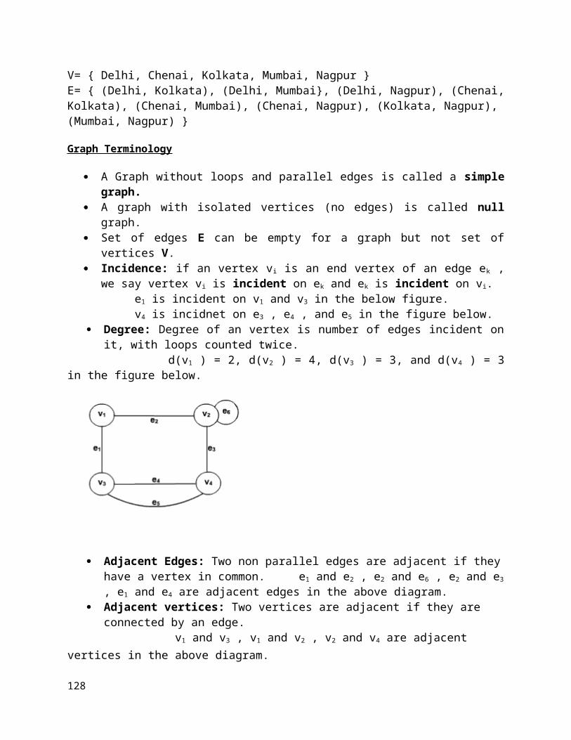
if( left==last-1 && arr[i]<arr[left] )/*right==last*/{

temp=arr[i];arr[i]=arr[left];arr[left]=temp;

}}

void main(){

int i;printf("Enter number of elements : ");scanf("%d",&n);for(i=0;i<n;i++){

printf("Enter element %d : ",i+1);scanf("%d",&arr[i]);

}printf("Entered list is :\n");

for(i=0;i<n;i++)printf("%d ",arr[i]);printf("\n");

create_heap();

printf("Heap is :\n");for(i=0;i<n;i++)printf("%d ",arr[i]);printf("\n");

heap_sort();

printf("Sorted list is :\n");for(i=0;i<n;i++)printf("%d ",arr[i]);printf("\n");getch();

}Radix Sort

128

In computer science, radix sort is a non-comparative integer sorting algorithm that sorts data with integer keys by grouping keys by the individual digits which share the same significant position and value. A positional notation is required, but because integers can represent strings of characters (e.g., names or dates) and specially formatted floating point numbers, radix sort is not limited to integers.

As an example, consider the list of integers:

36 9 0 25 1 49 64 16 81 4

n is 10 and the numbers all lie in (0,99). After the first phase, we will have: Bin 0 1 2 3 4 5 6 7 8 9

Content 0 181 - - 64

425 36

16- - 9

49

Note that in this phase, we placed each item in a bin indexed by the least significant decimal digit.

Repeating the process, will produce:

Bin 0 1 2 3 4 5 6 7 8 9

Content0149

16 25 36 49 - 64 - 81 -

In this second phase, we used the leading decimal digit to allocate items to bins, being careful to add each item to the end of the bin.

We can apply this process to numbers of any size expressed to any suitable base or radix.

Lecture-45 Linear and binary search methods

129

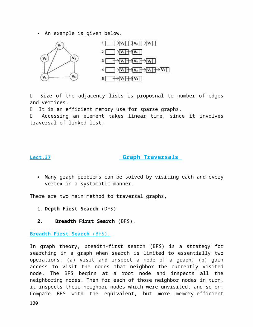
Binary searchIn computer science, a binary search or half-interval search algorithm finds the position of a specified input value (the search "key") within an array sorted by key value.[1][2] For binary search, the array should be arranged in ascending or descending order. In each step, the algorithm compares the search key value with the key value of the middle element of the array. If the keys match, then a matching element has been found and its index, or position, is returned. Otherwise, if the search key is less than the middle element's key, then the algorithm repeats its action on the sub-array to the left of the middle element or, if the search key is greater, on the sub-array to the right. If the remaining array to be searched is empty, then the key cannot be found in the array and a special "not found" indication is returned.

Program

#include <stdio.h> int main(){ int c, first, last, middle, n, search, array[100];  printf("Enter number of elements\n"); scanf("%d",&n);  printf("Enter %d integers\n", n);  for ( c = 0 ; c < n ; c++ ) scanf("%d",&array[c]);  printf("Enter value to find\n"); scanf("%d",&search);  first = 0; last = n - 1; middle = (first+last)/2;  while( first <= last ) { if ( array[middle] < search ) first = middle + 1; else if ( array[middle] == search ) { printf("%d found at location %d.\n", search, middle+1); break; } else last = middle - 1;

130

  middle = (first + last)/2; } if ( first > last ) printf("Not found! %d is not present in the list.\n", search);  return 0; }

Linear search

In computer science, linear search or sequential search is a method for finding a particular value in a list that consists of checking every one of its elements, one at a time and in sequence, until the desired one is found.

Linear search is the simplest search algorithm; it is a special case of brute-force search. Its worst case cost is proportional to the number of elements in the list; and so is its expected cost, if all list elements are equally likely to be searched for. Therefore, if the list has more than a few elements, other methods (such as binary search or hashing) will be faster, but they also impose additional requirements.

Program

#include <stdio.h> int main(){ int array[100], search, c, n;  printf("Enter the number of elements in array\n"); scanf("%d",&n);  printf("Enter %d integer(s)\n", n);  for (c = 0; c < n; c++) scanf("%d", &array[c]);  printf("Enter the number to search\n"); scanf("%d", &search);  for (c = 0; c < n; c++) { if (array[c] == search) /* if required element found */ { printf("%d is present at location %d.\n", search, c+1);

131

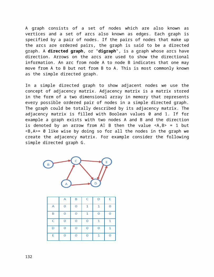
break; } } if (c == n) printf("%d is not present in array.\n", search);  return 0;}

Lecture -46 &47 Hashing Techniques    

132

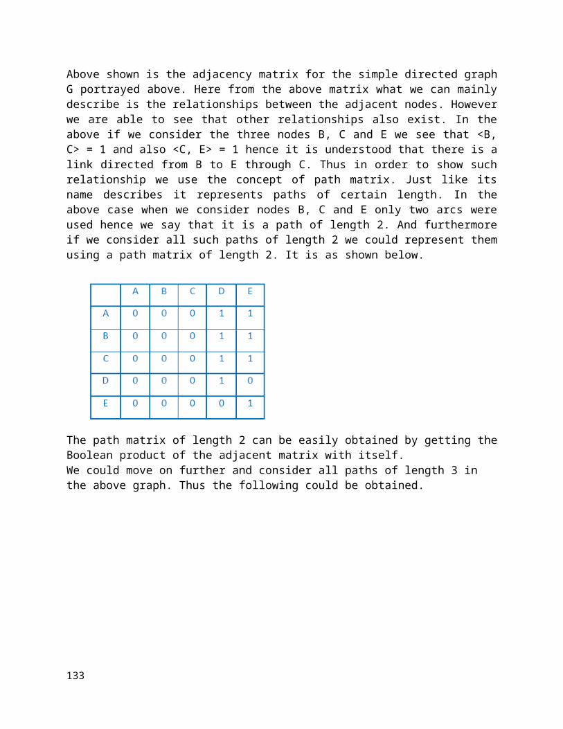
Hashing is a method to store data in an array so that sorting, searching, inserting and deleting data is fast. For this every record needs unique key.

The basic idea is not to search for the correct position of a record with comparisons but to compute the position within the array. The function that returns the position is called the 'hash function' and the array is called a 'hash table'.

WHY HASHING?

In the other type of searching, we have seen that the record is stored in a table and it is necessary to pass through some number of keys before finding the desired one. While we know that the efficient search technique is one which minimizes these comparisons. Thus we need a search technique in which there is no unnecessary comparison.

If we want to access a key in a single retrieval, then the location of the record within the table must depend only on the key, not on the location of other keys(as in other type of searching i.e. tree). The most efficient way to organize such a table is an array.It was possible only with hashing.

HASH CLASH  

Suppose two keys k1 and k2 are such that h(k1) equals h(k2).When a record with key two keys can't get the same position. such a situation is called hash collision or hash clash.

METHODS OF DEALING WITH HASH CLASH

There are three basic methods of dealing with hash clash. They are:

1. Chaining 2. Rehashing 3. Separate chaining.

CHAINING

It builds a link list of all items whose keys have the same value. During search, this sorted linked list is traversed sequentially from the desired key. It involves adding an extra link field to each table position. There are three types of chaining

1. Standard Coalsced Hashing 2. General Coalsced Hashing 3. Varied insertion coalsced Hashing

133

Standard Coalsced Hashing It is the simplest of chaining methods. It reduces the average number of probes for an unsuccessful search. It efficiently does the deletion without affecting the efficiency General Coalsced Hashing. It is the generalization of standard coalesced chaining method. In this method, we add extra positions to the hash table that can be used to list the nodes in the time of collision.

SOLVING HASH CLASHES BY LINEAR PROBING     The simplest method is that when a clash occurs, insert the record in the next available place in the table. For example in the table the next position 646 is empty. So we can insert the record with key 012345645 in this place which is still empty. Similarly if the record with key %1000 = 646 appears, it will be inserted in next empty space. This technique is called linear probing and is an example for resolving hash clashes called rehashing or open addressing.

DISADVANTAGES OF LINEAR PROBING

It may happen, however, that the loop executes forever. There are two possible reasons for this. First, the table may be full so that it is impossible to insert any new record. This situation can be detected by keeping an account of the number of records in the table.

When the count equals the table size, no further insertion should be done. The other reason may be that the table is not full, too. In this type, suppose all the odd positions are emptyAnd the even positions are full and we want to insert in the even position by rh(i)=(i+2)%1000 used as a hash function. Of course, it is very unlikely that all the odd positions are empty and all the even positions are full.

However the rehash function rh(i)=(i+200)%1000 is used, each key can be placed in one of the five positions only. Here the loop can run infinitely, too.

134

SEPARATE CHAINING

As we have seen earlier, we can't insert items more than the table size. In some cases, we allocate space much more than required resulting in wastage of space. In order to tackle all these problems, we have a separate method of resolving clashes called separate chaining. It keeps a distinct link list for all records whose keys hash into a particular value. In this method, the items that end with a particular number (unit position) is placed in a particular link list as shown in the figure. The 10's, 100's not taken into account. The pointer to the node points to the next node and when there is no more nodes, the pointer points to NULL value.

ADVANTAGES OF SEPERATE CHAINING

1. No worries of filling up the table whatever be the number of items. 2. The list items need not be contiguous storage

It allows traversal of items in hash key order.

CLUSTERING

There are mainly two types of clustering: 1. Primary clustering

When the entire array is empty, it is equally likely that a record is inserted at any position in the array. However, once entries have been inserted and several hash clashes have been resolved, it doesn't remain true. For, example in the given above table, it is five times as likely for the record to be inserted at the position 994 as the position 401. This is because any record whose key hashes into 990, 991, 992, 993 or 994 will be placed in 994, whereas only a record whose key hashes into 401 will be placed there. This phenomenon where two keys that hash into different values compete with each other in successive rehashes is called primary clustering. CAUSE OF PRIMARY CLUSTERING Any rehash function that depends solely on the index to be rehashed causes primary clustering WAYS OF ELEMINATING PRIMARY CLUSTERING One way of eliminating primary clustering is to allow the rehash function to depend on the number of times that the function is applied to a particular hash value. Another way is to use random permutation of the number between 1 and e, where e is (table size -1, the largest index of the table). One more method is to allow rehash to depend on the hash value. All these methods allow key that hash into different locations to follow separate rehash paths.

2. SECONDARY CLUSTERING   In this type, different keys that hash to the same value follow same rehash path.  

WAYS TO ELIMINATE SECONDARY CLUSTERING

135

All types of clustering can be eliminated by double hashing, which involves the use of two hash function h1(key) and h2(key).h1 is known as primary hash function and is allowed first to get the position where the key will be inserted. If that position is occupied already, the rehash function rh(i,key) = (i+h2(key))%table size is used successively until an empty position is found. As long as h2(key1) doesn't equal h2(key2),records with keys h1 and h2 don't compete for the same position. Therefore one should choose functions h1 and h2 that distributes the hashes and rehashes uniformly in the table and also minimizes clustering.

Lecture-48

136

Beyond Syllabus-Time complexity. Dijkstra’s algorithm

In computer science, the time complexity of an algorithm quantifies the amount of time taken by an algorithm to run as a function of the length of the string representing the input.Time complexity of an algorithm signifies the total time required by the program to run to completion. The time complexity of algorithms is most commonly expressed using the big O notation.

Time Complexity is most commonly estimated by counting the number of elementary functions performed by the algorithm. And since the algorithm's performance may vary with different types of input data, hence for an algorithm we usually use the worst-case Time complexity of an algorithm because that is the maximum time taken for any input size.

Calculating Time ComplexityNow lets tap onto the next big topic related to Time complexity, which is How to Calculate Time Complexity. It becomes very confusing some times, but we will try to explain it in the simplest way.

Now the most common metric for calculating time complexity is Big O notation. This removes all constant factors so that the running time can be estimated in relation to N, as N approaches infinity. In general you can think of it like this : statement;

Above we have a single statement. Its Time Complexity will be Constant. The running time of the statement will not change in relation to N.

for(i=0; i < N; i++){ statement;}The time complexity for the above algorithm will be Linear. The running time of the loop is directly proportional to N. When N doubles, so does the running time.

for(i=0; i < N; i++) { for(j=0; j < N;j++) { statement; }}This time, the time complexity for the above code will be Quadratic. The running time of the two loops is proportional to the square of N. When N doubles, the running time increases by N * N.

while(low <= high) {

137

mid = (low + high) / 2; if (target < list[mid]) high = mid - 1; else if (target > list[mid]) low = mid + 1; else break;}This is an algorithm to break a set of numbers into halves, to search a particular field(we will study this in detail later). Now, this algorithm will have a Logarithmic Time Complexity. The running time of the algorithm is proportional to the number of times N can be divided by 2(N is high-low here). This is because the algorithm divides the working area in half with each iteration.

void quicksort(int list[], int left, int right){ int pivot = partition(list, left, right); quicksort(list, left, pivot - 1); quicksort(list, pivot + 1, right);}Taking the previous algorithm forward, above we have a small logic of Quick Sort(we will study this in detail later). Now in Quick Sort, we divide the list into halves every time, but we repeat the iteration N times(where N is the size of list). Hence time complexity will be N*log( N ). The running time consists of N loops (iterative or recursive) that are logarithmic, thus the algorithm is a combination of linear and logarithmic.

NOTE : In general, doing something with every item in one dimension is linear, doing something with every item in two dimensions is quadratic, and dividing the working area in half is logarithmic.

Types of Notations for Time ComplexityNow we will discuss and understand the various notations used for Time Complexity.

1. Big Oh denotes "fewer than or the same as" <expression> iterations.2. Big Omega denotes "more than or the same as" <expression> iterations.3. Big Theta denotes "the same as" <expression> iterations.4. Little Oh denotes "fewer than" <expression> iterations.5. Little Omega denotes "more than" <expression> iterations.

Understanding Notations of Time Complexity with ExampleO(expression) is the set of functions that grow slower than or at the same rate as expression.

138

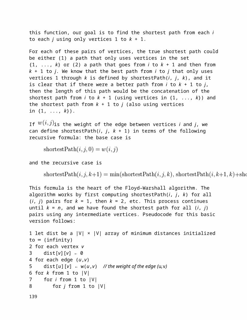
Omega(expression) is the set of functions that grow faster than or at the same rate as expression.

Theta(expression) consist of all the functions that lie in both O(expression) and Omega(expression).

Suppose you've calculated that an algorithm takes f(n) operations, where,

f(n) = 3*n^2 + 2*n + 4. // n^2 means square of nSince this polynomial grows at the same rate as n^2, then you could say that the function f lies in the set Theta(n^2). (It also lies in the sets O(n^2) and Omega(n^2) for the same reason.)

The simplest explanation is, because Theta denotes the same as the expression. Hence, as f(n) grows by a factor of n^2, the time complexity can be best represented as Theta(n^2)

Dijkstra’s algorithm

Dijkstra's algorithm solves the single-source shortest-path problem when all edges have non-negative weights. It is a greedy algorithm and similar to Prim's algorithm. Algorithm starts at the source vertex, s, it grows a tree, T, that ultimately spans all vertices reachable from S. Vertices are added to T in order of distance i.e., first S, then the vertex closest to S, then the next closest, and so on. Following implementation assumes that graph G is represented by adjacency lists.

DIJKSTRA (G, w, s)

1. INITIALIZE SINGLE-SOURCE (G, s)2. S ← { }     // S will ultimately contains vertices of final

shortest-path weights from s3. Initialize priority queue Q i.e., Q  ←  V[G]4. while priority queue Q  is not empty do5.     u  ←  EXTRACT_MIN(Q)    // Pull out new vertex6.     S  ←  S{u}

    // Perform relaxation for each vertex v adjacent to u7.     for each vertex v in Adj[u] do8.         Relax (u, v, w)

Analysis

Like Prim's algorithm, Dijkstra's algorithm runs in O(|E|lg|V|) time.

 

139

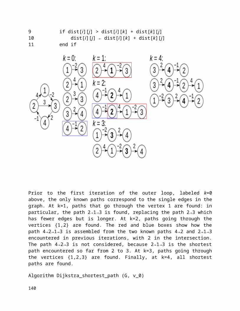
Example: Step by Step operation of Dijkstra algorithm.

 

Step1. Given initial graph G=(V, E). All nodes nodes have infinite cost except the source node, s,  which has 0 cost.

Step 2. First we choose the node, which is closest to the source node, s. We initialize d[s] to 0. Add it to S. Relax all nodes adjacent to source, s. Update predecessor (see red arrow in diagram below) for all nodes updated.

Step 3. Choose the closest node, x. Relax all nodes adjacent to node x. Update predecessors for nodes u, v and y (again notice red arrows in diagram below).

140

Step 4. Now, node y is the closest node, so add it to S. Relax node v and adjust its predecessor (red arrows remember!).

Step 5. Now we have node u that is closest. Choose this node and adjust its neighbor node v.

Step 6. Finally, add node v. The predecessor list now defines the shortest path from each node to the source node, s.

141

 

----------------------------------------------------- X X X ------------------------------------------------------

142