lecture notes for algorithm design - rutgers universitycrab.rutgers.edu/~guyk/alg.pdf · lecture...
TRANSCRIPT

Algorithms lecture notes 1
Lecture notes for algorithmdesign
Guy Kortsarz

Algorithms lecture notes 2
What are programs? What are algorithms?
What do they do?
Programs versus algorithms
A program is a finite collection of lines Every
line states a finite number of commands.
Every command must have a clear meaning
that a computer can execute.
A program has to be written in a computer
language.
Examples: LISP, C, C++, JAVA, PASCAL,
COBOL, FORTRAN, PROLOG, Python,
Algol (one of the very first)
What do programs do? They manipulate some
data we call The input and get some answer
called The output.
Thus programs create a mapping from inputs
to outputs.
So what is an algorithm? It is the high level
description of a program.
We use some universal syntax. A pseudocode.

Algorithms lecture notes 3
What is a combinatorial problem?
What do algorithms (and thus programs) solve?
Combinatorial problems (combinatorial is for
discrete)
A problem is not:
Not a riddle (like the one of the Sphinxes). Not
a direct information question (Where do the
ducks go in winter when the lake is frozen?).
The main difference is that our problems have
infinite many inputs and to each one exact
expected output. You will learn (theory of
computing) that a combinatorial problem with
finite number of inputs is a completely
absurd notion.
The program written has to be correct
(compute the correct function) on any input.
Exception: randomized algorithms.

Algorithms lecture notes 4
An example for a problem
Example:
Input: A collection of numbers
Required: The maximum
Note that we need to get it right regardless of
the input in the array

Algorithms lecture notes 5
An example
Input: 7, 2, 3, 1, 4, 8, 5, 4
The output: must be 8.

Algorithms lecture notes 6
PROGRAMS ARE NOT
ALLOWED IN HOMEWORK
You know how to program. This is not what I
am trying to teach.
One can describe answer via pseudocodes. A
universal syntax to be discussed.
An algorithm in fact is best described in words,
and at least toward the end I hope you will be
able to do it.
WARNING: IF YOUR ANSWER IS A
CODE IN ANY LANGUAGE, AT FIRST
YOU LOOSE POINTS AND LATER YOU
LOOSE ALL THE POINTS.
LEARN TO WRITE IN PSEUDOCODE OR
EXPLAIN IN WORDS.
For example for assignment we use x← y for x
gets the value in y

Algorithms lecture notes 7
Some issues we abstract when
writing an algorithm
1. Reading the input: We will assume that the
input was already read into the appropriate
variables. Usually in an array (see later).
2. The variable type is implicit in the
command. If the command is x← F (F
stands for False) then x is a boolean
variable. The type of a variable follows
from its context
3. The exact way to output is abstracted by
the command Return(). This exits the
algorithm and returns a solution.
We will use while and for loops like in
programs, and similarly we shall use the
If-then-else scheme. We also use recursion.

Algorithms lecture notes 8
Arrays
An array is a block of contiguous addresses in
the memory. An array is typically denoted
A[1..n]. We assume that it contains data
(usually numbers).
We assume that A starts at 1 and ends in n for
some n. For any 1 ≤ j ≤ n A[j] already has
some value. Getting to A[⌈n/2⌉] requires onetime unit.
A[7]← A[16] for example inserts the value of
A[16] into A[7].
A[7]← 16 puts the value 16 in A[7].
A typical input would be denoted as, for
example A < 7, 2, 3, 8, 9, 12,−4 >. In this case
n = 7 and A[4] = 8 etc.

Algorithms lecture notes 9
Segmentation mistakes
Say that n = 50. A command like
A[51]← A[50] creates unclear (machine
dependent) result. In UNIX that the computer
will stop the execution and will say
“Segmentation fault, core dumped”.
Segmentation: a wrong address.
The core records the run of the algorithm. In a
fatal error the core is removed (namely
dumped).

Algorithms lecture notes 10
Finding the maximum
The idea:
Go over the array from left to right
Maintain at each time the largest number
found so far.
Again: an algorithm is an idea.
1. M ← A[1]
2. For i← 2 to n do
(a) If A[i] > M then M ← A[i]
3. Return(M)

Algorithms lecture notes 11
Can we do with less than n− 1
comparisons?
The question is less simple than appeared.
Say that we partition the elements into pairs
and compare them.
And then continue.
Use transitivity (a < b and b < c to get a < c)
to try and derive less than n comparisons.
Is the above possible? The answer is no! Any
comparison based algorithm requires at least
n− 1 comparisons.
Why?: Every companions has a winner and
looser.
Hence call A[i] a looser if it lost in at least one
comparison.
After n− 2 comparisons there are at most
n− 2 losers (and even the n− 2 is true if no
element lost twice).
So at least 2 elements never lost. So we cant
tell which one of them is the maximum.

Algorithms lecture notes 12
Average and worst case: Searching
for x in A[1..n]
1. Found← F
2. i← 1
/* This is an initialization: we set the
boolean variable found to “not yet” /*
3. While not(Found) do:
(a) If A[i] = x then Return(i)
/* The case x was found */
(b) Else, i← i+ 1
/* Contrary to the for loop, the
program is required to augment i */
4. Return(”x is not in A”)
Assuming x ∈ A then the average case is n/2.
The worst case is n− 1 comparisons.

Algorithms lecture notes 13
Recursion
A program that calls itself.
For example to compute n!
Fact(n)
1. If n = 1 return 1
2. Else return n · Fact(n− 1)
If you give it a negative integer, an infinite
loop.

Algorithms lecture notes 14
Reversing a string
Say that A has a collection of characters that
we want to reverse
We wil assume that given two strings (as
arrays) there is a command conc that
concatenate the two strings to one string
namely two arrays to one.
conc(< g, e, t, l, o >< s, t >)
=< g, e, t, l, o, s, t >.
Reverse(A[1, n])
1. if n = 1 return A
2. Return
conc(A[n], Reverse(A < 1..n− 1 >))

Algorithms lecture notes 15
Example
Example: A < d, i, p, u, t, s >
We get < s > ·Revers(d, i, p.u, t) =< s, t >
·Reverse(s, i, p, u) =< s, t, u >
·Reverse(d, i, p) =< s, t, u, p >
·Reverse(d, i) =< s, t, u, p, i > ·Reverse(d) =<
s, t, u, p, i, d >.

Algorithms lecture notes 16
Finding the maximum in an
increasing decreasing sequence
An increasing decreasing sequence is an array
of numbers that increases to a certain point
and then starts decreasing.
Examples:
2, 8, 13, 25, 23, 22, 20, 7, 1
4, 5, 9, 12, 40, 50, 80, 81
Thus, an increasing sequence is also
increasing-decreasing
21, 13, 9, 4, 2, 1
And so is a decreasing sequence
To find the maximum we may scan the list
from left to right
As soon as A[i] > A[i+ 1] we may return A[i]
But in the worst case (which is our concern) its
still n− 1 comparisons
Can we do better?

Algorithms lecture notes 17
Reducing from n to log n
We will define log n later. For now think of it
as a very small function of n. The following
algorithm does much better.
The idea: compare the two middle elements
If the sequence still increases choose the right
half (the left half is discarded)
Else, choose the left half (half of the elements
are discarded)
1. left← 1; right← n
2. While left < right do:
(a) middle← ⌊(left+ right)/2⌋(b) If A[middle+ 1] > A[middle]
left← middle+ 1
(c) Else right← middle
3. Return(A[left])

Algorithms lecture notes 18
GO TO LEFT HALF
GO TO RIGHT HALF

Algorithms lecture notes 19
A run of the algorithm
7 13 17 22 28 36 42 16 9 7 2 −3
1 2 3 4 5 6 7 8 9 1110 1312
left right
7 13 17 22 28 36 42 16 9 7 2 −3
7 13 17 22 28 36 42 16 9 7 2 −3
49
49
49
right
rightleft
7 13 17 22 28 36 42 49 16 9 7 2 −3
rightleft
7 13 17 22 28 36 42 49 16 9 7 2 −3
left
right
left

Algorithms lecture notes 20
The number of comparisons
Each time a comparison is made the number of
remaining elements becomes at most 1/2 the
current. log n is the number of times you can
divide a number by 2 until it gets to 1.
For example: n = 128, n = 64, n = 32, n =
16, n = 8, n = 4, n = 2, n = 1
Thus, starting with 128 after 7 times we divide
by 2 we get 1
Thus: log2 128 = 7 or 27 = 128
log2 n = x is equivalent to 2x = n
The log n function, examples:
log2 1024 = 10
log2 106 is roughly 20.
log2 1012 is roughly 40
Let x = 2300. x > number of atoms in the
known universe. log2 x = 300.
Thus log n increases very slowly and for large
enough n: any constant < log n <<< n

Algorithms lecture notes 21
The log: slowly increasing function
The log2 n is the exponent we need to get to n.
Namely 2log2m = m.
The relation between n and log n is like
between n, 2n
⌈log n⌉ is the number of binary bits required to
represent n
The value ⌈log2 n⌉ is also the number of times
we can divide n by 2 until we get to 1.
The log n function is not constant
But grows very slowly
Thus n · log n << n2
But n < n · log n
Algorithms lecture notes 22
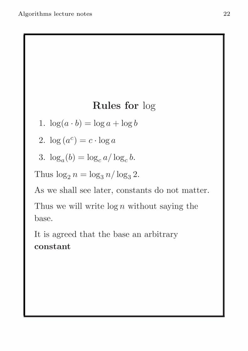
Rules for log
1. log(a · b) = log a+ log b
2. log (ac) = c · log a
3. loga(b) = logc a/ logc b.
Thus log2 n = log3 n/ log3 2.
As we shall see later, constants do not matter.
Thus we will write log n without saying the
base.
It is agreed that the base an arbitrary
constant
Algorithms lecture notes 23
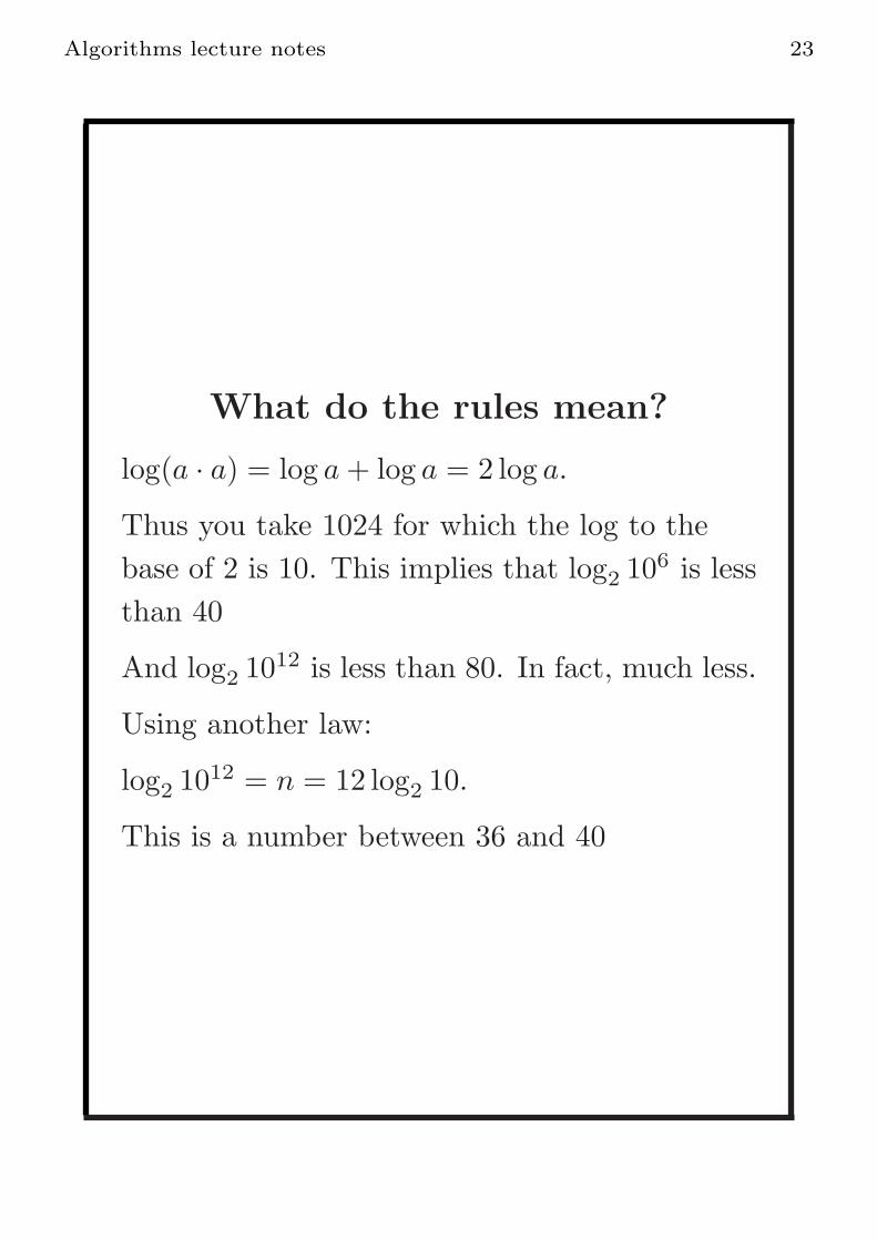
What do the rules mean?
log(a · a) = log a+ log a = 2 log a.
Thus you take 1024 for which the log to the
base of 2 is 10. This implies that log2 106 is less
than 40
And log2 1012 is less than 80. In fact, much less.
Using another law:
log2 1012 = n = 12 log2 10.
This is a number between 36 and 40

Algorithms lecture notes 24
If the input is a single number p
what is the size?
We use a binary representation.
The representation requires ⌈log p⌉. That ishow much space it takes to represent the single
number. Hence that is the size of the input.
If the input is a number and an algorithm runs
in time Θ(p) or Θ(√p) it is not a polynomial
time algorithm.

Algorithms lecture notes 25
A single number as input
p = 2log p
√p = p1/2 = 2log p/2 =
√2pwhich is
exponential.
Definition: An exponential algorithm.
Runs in time cpoly(n) for a constant c > 1 with
n the size of the input. Thus 2p is exponential
time.
In fact, only polynomial time algorithm (more
precisely algorithm whose run time is bounded
by a polynomial in the size of the input) are
consider tractable.
If the input is just p, a polynomial algorithm
would be for example an algorithm that runs in
time O((log p)4)

Algorithms lecture notes 26
Running time for algorithms: a
definition
1. We count basic operations ·,+←, if, . . .
not time
/* Time is machine dependent. All
operation 1 time unit */
/* Maybe its not fair to say that very basic
command takes one unit */
/* However today multiplication takes as
much time as addition */
2. The running time is as a function of the
size (which is more or less number of items
unless the input contains huge numbers)
/* Running times will be bounded by some
function of the size n. For example 7n2 or√n/ logn */
3. We always compute the running time for
the worst case of the algorithm.
/* This is a political, namely, subjective,
decision */

Algorithms lecture notes 27
What is not important?
1. Low order terms are ignored
/* Example: a polynomial of rank is d,
implies time is nd */
/* We need later a way to find out who is
the leading term */
2. Constant do not matter except in the
exponent.
/* Constants can be overcome by a faster
computer */
3. If you have a sum of finite many terms
only the leading term defines the function
4. All these things are suspect from a
practical view
/* For example: In practice bad constant
can ruin an algorithm */

Algorithms lecture notes 28
The theoretical running times and
their problems
An algorithm that is faster than another is
indeed faster in a very narrow sense.
/* In the worst case and perhaps for very large
n */
/* This is true regardless of the computer that
the algorithm runs on */
/* Because the speed difference between
computers is constant */
The worst case assures us that the number of
operations is never more than what we
computed
/* Yes, but it may not reflect the typical
running time */
The worst case is easier to analyze than the
average case
/* Yes, but harder to analyze does not mean
its not a better definition */

Algorithms lecture notes 29
Continued
The Algorithm called Quicksort is the best
sorting algorithm in practice to sort numbers
from small to large.
Better than the (theoretically better) Mergesort
The reason: Quicksort is better on average
(smaller constants).

Algorithms lecture notes 30
How does Quicksort and
Mergesort compare
QUICKSORT
MERGESORT
SAYING MERGESORT IS BETTER MAY BE UNFAIR.

Algorithms lecture notes 31
Bubble-sort
Bubble-sort(A)
1. For i← 1 to n− 1 do:
(a) For j ← 1 to n− i do if A[j + 1] < A[j]
Swap A[j] and A[j + 1]
2. Return(A)
We constantly scan the array from left to right
Check if A[1] smaller than A[2] and if so swap
them, then if A[2] smaller than A[3] and swap,
if so, etc.
After the first round, the maximum is at the
end.
After i rounds, the last i numbers are correct

Algorithms lecture notes 32
An example of a run
12 3 7 5 14 13 10486 2
3
AN EXAMPLE FOR A RUN OF THE ALGORITHM
3 6 4 7 58
3
3 4 2
3 4 5 2 8 10 12 13 14 15
13 10 14
5
5
5 6 4
122
7 5 2 8 14131012
5 4 6 5 2 7 8 10 12 13 14
5 5 6 7 8 10 12 13 14
5 6

Algorithms lecture notes 33
Running time
In first round n− 1 comparisons
In second round n− 2.
In general
1 + 2 + 3 + . . . (n− 1)
It turns out that:
((n− 1) + 1) = ((n− 2) + 2) = ((n− 3) + 3) . . .
Thus the sum if n(n− 1)/2
Thus running time n2 because constants are
ignored
Reverse sorted array shows the time is Θ(n2).

Algorithms lecture notes 34
Insertion sort
Another basic sorting algorithm:
Insertion− Sort(A)
1. For i = 2 to n do:
/* Put A[i] in its proper place on the
sorted array A[1 . . . i−] */(a) rp← i
(b) While rp > 1 and A[rp− 1] > A[rp]
Do:
(c) i. Swap A[rp] and A[rp− 1]
ii. rp← rp− 1
2. Return(A)

Algorithms lecture notes 35
An example of a run
12 3 7 5 14 13 1048156 2
3
AN EXAMPLE FOR A RUN OF THE ALGORITHM
3
3
3 6
3 4
12 6
12
15 8 4 7 5 2 14 13 10
6 15 8 4 7 5 2 14 13 10
6 8 12 15 4 7 5 2 14 13 10
8 12 15 7 5 2 14 13 104
6 7 8 12 15 5 2 14 13 10

Algorithms lecture notes 36
Finding 17 via binary search
3 7 14 17 21 22 14 26 32 35 40
3 7 14 17
13
13
O(LOG N) RUNNING TIME
1 2 3 4 5 7 8 9 11 12
14
10
17
17

Algorithms lecture notes 37
O(),Ω, Θ()
If the running time is n2 or less up to constants
we denote that by T (n) = O(n2)
Very bad notation T (n) = O(n2) means T (n) is
at most n2 up to constants. For example
n = O(n2). Its ≤ and not equal.
Ω(n2) at least n2 up to constants.
Θ(n2) means both O() and Ω(). Real equality.
A formal definition:
f(n) = O(g(n)) iff there exists c, so that for
every n f(n) ≤ c · g(n).

Algorithms lecture notes 38
Example
For 100 · n ≤ c · n2/100.
Choose c = 10000. This gives
100 · 100 · n ≤ 100000 · n2 and this is true.
Many time O() is defined with a multiplicative
and an additive constants so that the
constant will not be too large.
For simplicity, I avoid that.
Example: a polynomial is Θ(nd) with d the
highest exponent.

Algorithms lecture notes 39
Discussion
O is at most Ω() is at least and Θ() means the
same.
We say that f(n) = Θ(g(n)) if f(n) = O(g(n))
and g(n) = O(f(n))
if f(n) = O(g(n)) then g(n) = Ω(f(n)).
A new definition.
f(n) = o(g(n)) if f is strictly less than g(n)
namely f(n) = O(g(n)) holds and
g(n) = O(f(n)) is not true.
For example n = o(n logn).
1000 · n = o(n · log n).

Algorithms lecture notes 40
Theoretical running time is
important for your grade
1. For us there is only worst case.
2. This is a course in theory
3. If you can have a time Θ(n · log n)algorithm versus and Θ(n2) algorithm the
first is BETTER IN THIS COURSE.
4. In fact, the slower algorithm from a
theoretical point of view WILL NOT GET
ALL POINTS!
5. Another example (Maybe) in biology
theory fits, as in the DNA n is huge.
If you want, check the Data Structure lecture
notes. They have an exercise that practices
comparing the order of magnitude of functions.

Algorithms lecture notes 41
Selection sort
Consider an algorithm that sorts like that: It
finds the maximum, puts it in the end. Then
sets the end of the array to n− 1. Find the
new maximum and put it in place n− 1 and so
on. What is the best average and worst case of
this algorithm
All the there running times are the same. Its
for loops.
At the beginning we make n− 1 comparison
After that n− 1 and so on
So Θ(n2) running time

Algorithms lecture notes 42
General techniques for solving
algorithms: Exhaustive search
Input: and array A and a number S.
Question: are there A[i], A[j], i 6= j so that
A[i] +A[j] = S
1. For i = 2 to n do:
(a) For j = 1 to i− 1 do: If A[i] +A[j] = S
return ”Yes”
2. Return ”No”
Trying all pairs. Going over all possible
candidate solutions.

Algorithms lecture notes 43
Exhaustive search
For a question that asks what is the best
ordering on a line, the number of possibilities is
n!.
When the answer is a subset, 2n possibilities.
Choosing all subsets of size k is(
nk
)
which
equals roughly 2n for k = n/2
In general exhaustive search is what you do
when you do not have any good idea.
Algorithms lecture notes 44
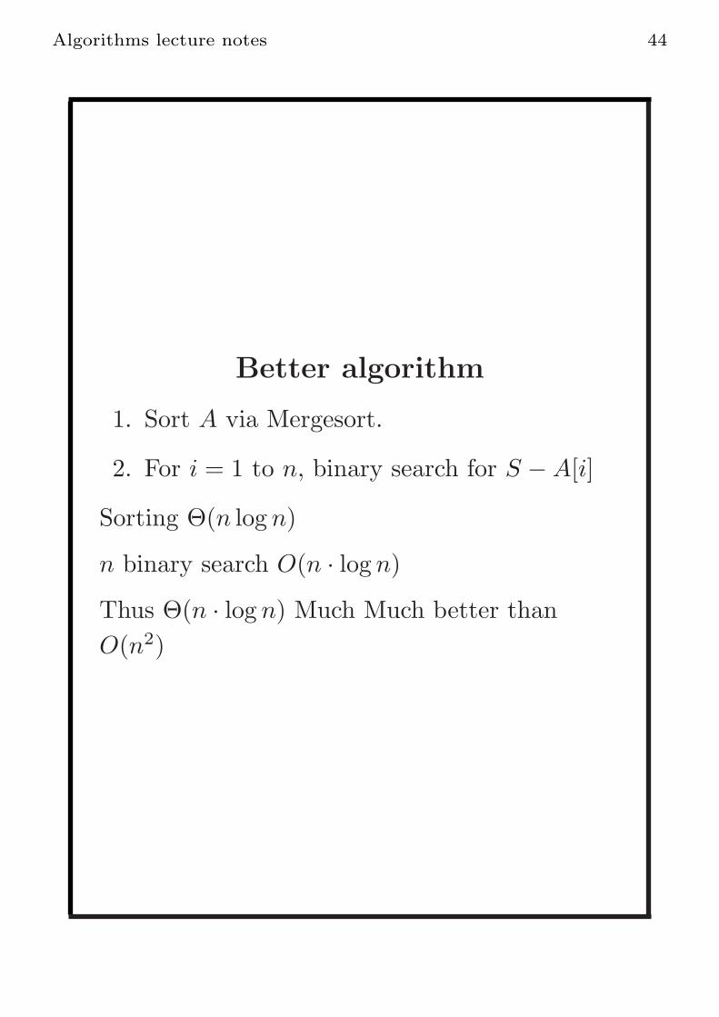
Better algorithm
1. Sort A via Mergesort.
2. For i = 1 to n, binary search for S −A[i]
Sorting Θ(n logn)
n binary search O(n · log n)Thus Θ(n · log n) Much Much better than
O(n2)

Algorithms lecture notes 45
Divide and conquer
1. Partition P into say 2 Disjoint problems
P1, P2
2. Solve P1, P2 by recursion
3. A merge step: get a solution for P based
on the solution for P1, P2.
The disjointness is critical

Algorithms lecture notes 46
Example: The height of a binary
tree
Let p be a pointer to the root.
Let left(p) and right(p) be the pointers to the
left and right child of p.
The height is the longest path from a root to a
leaf (a path goes from a child to a parent or
vice versa).
Algorithm Height(p)
1. If p = null Return(−1)
2. Else Return
maxHeight(left(p)), Height(right(p))+1.

Algorithms lecture notes 47
How is the height defined
H−1 H−7
(H−1)+1=H

Algorithms lecture notes 48
A partial run of the algorithm
A
B
1
2
C
3
4
56
7
8
D
E
F
X
Y
W P
9
10
11
12
1314
15
16
H=0
H=1
17
18
19
20
H=1
H=2
H=3

Algorithms lecture notes 49
The number of the vertices of a
tree
Algorithm Num(p)
1. If p = null Return(0)
2. Else Return
Num(left(p)) +Num(right(p)) + 1.

Algorithms lecture notes 50
The number of leaves in a tree
Algorithm Leaves(p)
1. If p = null Return(0)
2. If left(p) = right(p) = null return 1
3. Else Return
Num(left(p)) +Num(right(p)).

Algorithms lecture notes 51
The longest path in the tree
Let p be a pointer to the root.
Try to write an algorithm for this.
You will need for any tree to keep both its
height hℓ, hr and its diameter Diam(p).
Note that if the diameter does not go via r the
diameter is simply
maxDiam(left(p)), Diam(right(p)).If the diameter goes via r, then it equals
h(left(p)) + h(right(p)) + 2.
You simply compare these two quantities and
return the largest one.

Algorithms lecture notes 52
Divide and conquer: Quicksort
The input A[ℓ, r] for ℓ ≤ r. We call the
algorithm globally ℓ = 1 and r = n.
Algorithm A[ℓ, r]
1. If ℓ = r return A
2. Let p be the number of elements less than
or equal A[ℓ]
3. Put all numbers less than or equal to A[ℓ]
(but A[ℓ]) in places ℓ, ℓ+ 1, . . . , ℓ+ p− 1.
4. Put A[ℓ] in A[p]
5. Put the rest of the number in places
p+ 1, p+ 2, . . . , r
6. Quichsort[ℓ, ℓ+ p− 1]
7. Quicksort(p+ 1 + ℓ, r]
8. Return(A)
Can cause infinite loop if A[ℓ] is either the
maximum or the minimum.
We avoid that by taking A[ℓ] from the array of
the small ones, and from that of the big ones.

Algorithms lecture notes 53
How does the divide and conquer
go?
The divide does most of the work. Divides to
smaller than A[1] and larger than A[1] which
requires Θ(n).
The conquer: recursion.
The merging: trivial.

Algorithms lecture notes 54
A run of Quicksort
5, 7, 6, 4, 1, 9, 2, 10, 3, 8
4, 1 ,2 3 5 97, 6, , 10, 8
1,2,3 4 5 6 7 9 , 10 , 8
1 2, 3 4 5 6 7 8 9 10
1 2 3 4 5 6 7 8 9 10

Algorithms lecture notes 55
A bad example: sorted array
1 2 3 4 n
2 3 41
1 2 3 4 5
2) In the worst case.SHOWING THAT QUICKSORT RUNS IN TIME O(n
Algorithms lecture notes 56
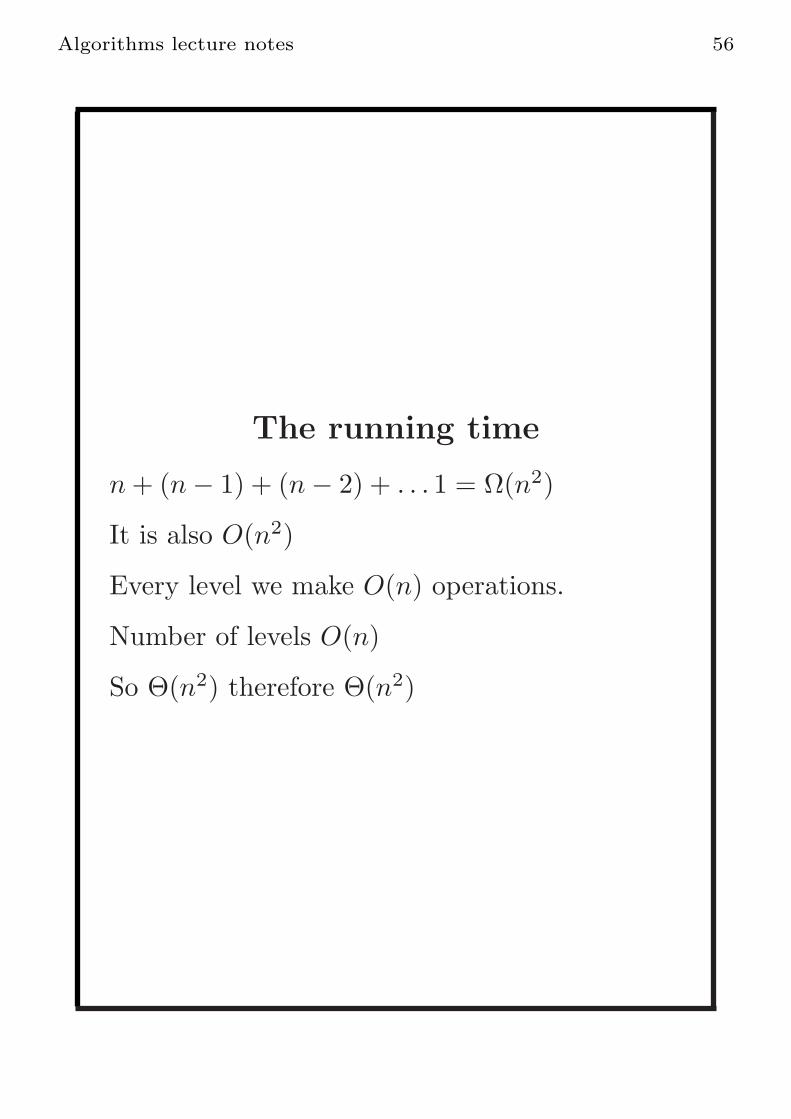
The running time
n+ (n− 1) + (n− 2) + . . . 1 = Ω(n2)
It is also O(n2)
Every level we make O(n) operations.
Number of levels O(n)
So Θ(n2) therefore Θ(n2)

Algorithms lecture notes 57
Divide an conquer: Mergesort
How to merge two sorted arrays
1. While BOTH A and B have elements do;
(a) If A[1] > B[1] Add B[1] to the end of C,
remove B[1] from B
/* This means that B[2] becomes B[1]
/*
(b) Else add A[1] to the end of C and
remove A[1] from A
(c) While A has elements do: add A[1] to
to the end of C and remove A[1] from A
(d) while B has elements do Add B[1] to
the end of C and remove B[1] from B
2. Return C

Algorithms lecture notes 58
Mergesort
Mergesort(A < i..j >)
1. if i = j Return(A)
2. Mergesort(A < i, ⌈(i+ j)/2⌉ >)
3. Mergesort(A < ⌈(i+ j)/2⌉+ 1, j >
4. Merge the two sorted arrays and return the
resulting array.
We call it with i = 1 and j = n.

Algorithms lecture notes 59
How does the divide and conquer
work here?
The divide is trivial.
The recursion is costly as usual
But the merge step is the one that does most of
the work.
At the end merges two disjoint arrays of size
n/2 each and this takes θ(n) operations.
In binary trees the divide is given for free and
the merge is usually one line

Algorithms lecture notes 60
A run of Mergesort
10 7 4 3 11 2 7 6
7 10 3 42 11 6 7
3 4 7 102 6 7 11
2 3 4 6 7 10 117

Algorithms lecture notes 61
The running time of Mergesort
n
n/2 n/2
n/4 n/4 n/4 n/4
n/8 n/8 n/8 n/8 n/8 n/8 n/8 n/8

Algorithms lecture notes 62
Greedy algorithm
Say for example that we want to find a ”good”
subset.
A greedy algorithm will go over the elements
and at every moment chooses the element that
seems the best now.
Seems unlikely that such a ”local” strategy
would work. But it does for many problems.
Showing that a greedy algorithm is optimal:
Always the same way.
Let A be the set of elements chosen so far.
We need to prove: There exists some OPT so
that A ⊆ OPT .
In greedy you do not delete so one wrong move
and you are done.
Like in ”Riding in Cars with Boys”.
Algorithms lecture notes 63
Coin Exchange
Input: An integer n and the definition of legal
coins.
Output: A collection of coins that adds to n.
We always assume that there is a coin of value
1 so that there always be a solution.
1. R← n; L ← ∅.
2. While R > 0 do
(a) Let c be the largest coin value so that
c ≤ R
(b) Add c into the solution L.(c) R← R− c
3. Output L.

Algorithms lecture notes 64
Example
T=66
We choose 25 twice.
What remains is 16
We choose 10 once.
What remains is 6.
We choose 5 once
And then 1 once.

Algorithms lecture notes 65
A proof that it works for America
coins
The America coins lets say 1, 5, 10, 25.
This implies some rules:
1. There are at most 4 1, as otherwise replace
with a 5.
2. The 1, 5 can be at most 9 otherwise we
replace by 10.
3. The 1, 5 and 10 can get to at most 24 as
otherwise replace by 25,
4. This implies the greedy algorithm is
correct. For example, as long as x ≥ 25
take 25 because the others sum to only 24.
And the same for taking 10 and taking 5

Algorithms lecture notes 66
But does it work in Sweden?
For the sake of example let the coins be 1, 5, 11.
Let us say that we want to get to 15
The greedy will take one 11 and 4 1.
The optimum takes 3 times 5.
The greedy does not work for any set of coins.
Works for example if all numbers are a power
of some constant.

Algorithms lecture notes 67
Maximum independent set on a
tree
In a rooted tree we say that a set is
independent, if no vertex and its parent belong
to the set.
Say that we need to choose who to invite to a
party but P (v) and v can not be invited
together (because they hate each other).
We may assume the following simple property:
Every leaf in the tree belongs to the
independent set.
Otherwise let ℓ be a leaf. Why is it not in the
independent set? P (ℓ) must be there.
Remove P (ℓ) and add ℓ
The value is still optimal.
Thus this works: put all leaves in, remove all
their parents and recurse. The running time is
O(n)

Algorithms lecture notes 68
An example of a run of the
algorithm
A
B
C
D
E
FG
H
K
L
M
N
OP
Q
R
S
TU
V
W
X
Z
J
Y
I

Algorithms lecture notes 69
What remains
C
V
W Z
Y
I

Algorithms lecture notes 70
Activity selection
We have a factory and a machine.
Clients ask for maintenance starting at a
certain time.
We know how much each job takes. So this
defines an interval [si, fi] for job i: si is the
time the costumer asked to start and fi − si is
the time it takes to start to finish of the
maintenance of job i.
Say that we have an interval [2, 5].
Say that there is another client its interval is
[4, 6].
Since there is only one machine, we can not
choose both of them.

Algorithms lecture notes 71
Problem definition continued
Two jobs that can be selected together are
called independent jobs. An independent set is
a collection of jobs so that every two are
independent.
If si, fi and sj , fj are independent then either
fi ≤ sj or fj ≤ si. Equality still means
independence.
Every job pays a dollar. The problem:
Input: A collection of intervals (si, ti)ki=1.
Objective: Find a maximum size independent
set

Algorithms lecture notes 72
An example of an input for the
activity selection problem
A B
C
D
E
F G H
I
A B EG H

Algorithms lecture notes 73
A good rule of thumb?
Some rules do not work such as choose the
shortest interval and remove the conflicting
interval and iterate.
Also does not work ”Choose the interval that
intersects the minimum number of intervals”
does not work. The counter example a bit big.
Also does not work: choose an interval that
starts first remove its neighbors and iterate.

Algorithms lecture notes 74
Rules that do not workCHOSING THE SHORTEST DOES NOT WORK
CHOOSING THE ONE WHO STARTS FIRST DOES NOT WORK

Algorithms lecture notes 75
Let L be the legal for addition
intervals (or Superman)
Algorithm: If the graph has one interval or
none, its the stopping condition.
In general:
1. L ← I
2. S ← ∅
3. While L 6= ∅ do(a) Add to S the interval I in L that ends
first
(b) Remove from L all intervals that
intersect I
4. Return S

Algorithms lecture notes 76
A run of the algorithm, example
A B
C
D
E
F G H
I
A B EG H
CHOOSE A REMOVE C CHOOSE B REMOVE D CHOOSE E REMOVE F CHOOSE GREMOVE I CHOOSE H

Algorithms lecture notes 77
Why does it work?
Its always the same proof. For every subset of
intervals S we need a witness that is some
OPT so that S ⊆ OPT .
Given an instance of the activity selection
problem, let I be the interval to end first
(breaking ties arbitrarily).
Then there exists an optimum that contains
I.

Algorithms lecture notes 78
The reason it works
X Z
Y
Y CAN NOT INTERSECT Z FOR OTHERWISE X END FIRST.
THIS MEANS THAT Y INTERSECTS EXACTLY ONE INTERVAL IN OPT
REMOVE
THUS THERE IS AN OPT CONTAINING Y
X FROM THE ABOVE AND ADD Y
Algorithms lecture notes 79
New witness
Let OPT1 be the witness that contains S.
Set OPT2 ← OPT1 + Y −X
We removed one interval and added another
one hence still optimum.
And contains Y .
By the same reasoning, at every stage we can
add the interval to end first from L.Hence the algorithm is optimal

Algorithms lecture notes 80
Gas pumping
Say that k cars come at the same time to a Gas
station that has only one machine.
Say that every car has a filling time si.
If the cars are treated in the order 1, 2, . . . n
then car i has to wait Fi =∑i−1
i=1 si
Give a greedy algorithm that minimizes the
sum of waiting times∑k
i=1 si.
Any suggested strategy?

Algorithms lecture notes 81
Huffman trees
We represent, say, the English alphabet. 26
letters. But also a versus A, etc. So 52
The characters ‘0′, ‘1′, . . . ‘9′ (not the numbers)
And many other symbols such as:
&, %, #, $
and so on.
There exists a standard code. The ASCII code.
American Standard code for information
interchange.
Since 8 bits we may represent up to 128
characters
The eight bit was first designed to be a check
bit (this is why 128 not 256). But now was
extended to 256.

Algorithms lecture notes 82
Some examples
00000000 is the Null character
00000001 is the start of a header
00000011 a character that marks the end of
text
The letter of a to z are: 01100001 to 01111010
in a contiguous way.
In many languages you can do “a”− “b” = 1
The capital letters are A = 01000001 and then
contiguous.
An extension exists known as Unicode
216 > 65000 characters

Algorithms lecture notes 83
Compressing: Huffman
Compression (save space) is important.
For example, in a DNA sequence instead of
writing AAAAAAAA, write A8.
But, more frequent is the need to compress
texts.
Letter do not have the same frequency. Clearly
A, a appear more than X,x
Hence in saving space we should give frequent
letters smaller codes
Every text may be different (frequency of
letters may vary) and so some times you
compress only after computing the frequencies.
The optimal compression method according to
frequencies is due to Huffman

Algorithms lecture notes 84
The difficulty with varying sizes
How would the computer know when a letter
ends
It will have a table with codes of letters.
But what happens if A=001, B=0011? How
can the computer tell them apart?
Rule: any code of a letter is not the beginning
(prefix) of the code for another letter.
To do this we use : Hierarchical trees

Algorithms lecture notes 85
I
XZ
E A
O
B
0 1
0 1 0 1
0 1 0 1
01

Algorithms lecture notes 86
Reading the codes
The paths from root to leaf would be the code.
I = 00, E = 010, A = 011, O = 10, B =
110, X = 1110, Z = 1111
The idea: frequent letters should get small
code.
Frequent, depends on the specific text
Not enough, many times, as the application is
typically “on-line” /Inorder
Lempel-Ziv: well known on-line compression
Algorithms lecture notes 87
A systematic way to create the tree
The tree is built from the leaves up
Each time, choose two (super)vertices with
lowest frequency and make them brothers
(sisters siblings).
A greedy algorithm as goes for the two lowest.
Making two letters sibling means that the path
until their parent would be equal
Which two letters should we “unite” first?
Clearly, the two less frequent
If A,B unit then create a virtual letter called
AB with frequency equal to sum of frequencies
Then continue in the same way

Algorithms lecture notes 88
A specific input
Note: the numbers sum to 1.
f(X) = 0.05, f(Y ) = 0.05, f(A) = 0.1, f(Z) =
0.2, f(B) = 0.2, f(C) = 0.4,
What is the optimal code?

Algorithms lecture notes 89
The resulting tree
X Y
XY A
XYA
0
0
1
1
Z B
ZB
XYAZB
01
C
XYAZBC
01
01
0.05 0.05
0.1
0.1
0.2
0.2 0.2
0.4
0.4
0.6

Algorithms lecture notes 90
Prolog for Dynamic programing
Computing Fibonacci numbers
F0 = 0, F1 = 1. F [i] = F [i− 1] + F [i− 2].
0, 1, 1, 2, 3, 5, 8, 13, 21 . . ..
A recursive algorithm
Fib(n)
1. If n ≤ 1 return n
2. Else return Fib(n− 1) + Fib(n− 2)
This is a terrible algorithm.
I got the bomb.

Algorithms lecture notes 91
The problems are not disjoint.
Recomputing which is not required
6
4 5
43 2
2 1 1 0
1 0
Computing over and over again the same things.

Algorithms lecture notes 92
What is the running time?
The running time is actually the n Fibonacci
number.
It is very close to ((1 +√5)/2)
n
Exponential algorithms certainly never
allowed.
In fact remember that we defines an algorithm
as acceptable if it is bounded by a polynomial
in the input.

Algorithms lecture notes 93
Serial Fibonacci
Ser − Fib
1. Sec← 0, Fir ← 1
2. For i← 1 to n− 2 do:
(a) tmp← Sec
(b) Sec← Fir
(c) Fir ← tmp+ Second
3. Return Fir
The running time is linear in n.

Algorithms lecture notes 94
Dynamic programming in general
Say that we try divide and conquer but the
problems are not disjoint.
Imagine you do the recursion in our head.
The tree may be huge. But with few entries
that appear again and again and again.
If we are lucky, the subproblems that you need
to solve are few and just appear many times.
The number of states the recursion can
generate is the number of possible different
recursive call.
In the recursion of Fib(n), F ib(n− 1) the
number of subproblems is only n:
Fib(1), F ib(2), . . . , F ib(n).
Many cases an exponential tree with very few
values return again and again.
Do not recompute them.

Algorithms lecture notes 95
The golden ticket example
The input is a line of stores.
Let us call these stores by 1, 2 . . . n
Store i wants to give you ci golden tickets.
A rule: you can choose stores i and i+ 1 as its
rude.
We go to our n is inside the solution or is not.
The maximum for n. If n 6∈ Sol then
sol[n− 1] = sol[n]
Otherwise sol[ln] = cn + sol[n− 2].
Every problem that can appear in the recursion
tree is just defined by [1, 2 . . . i].

Algorithms lecture notes 96
Golden ticket algorithm
1. A[1]← c1.
2. A[2]← maxA[1], c2.
3. For i = 3 to n do
A[i]← maxA[i− 1], A[i− 2] + ci
4. Return A[n]

Algorithms lecture notes 97
Example
c1 = 3, c2 = 2, c3 = 4, c4 = 2, c5 = 6, c6 =
1, c7 = 9, c8 = 10, c9 = 6, c10 = 9, c11 = 3
A[1] = 3, A[2] = 3
A[3]← max3, A[1] + 4 = 7.
A[4]← max7, A[2] + 2 = 7.
A[5]← max7, A[3] + 6 = 13.
A[6]← max13, A[4] + 1 = 13
A[7]← max13, A[5] + 9 = 22.
A[8]← max22, A[6] + 10 = 23.
A[9]← max23, A[7] + 6 = 28.
A[10]← max28, A[8] + 9 = 32.
A[11]← max32, A[9] + 3 = 32.
Algorithms lecture notes 98
Minimum steps to 1
Say that given a positive integer we are allowed
to make one of the 3 possible actions:
1. n← n− 1
2. If 2 divides n we can set n← n/2
3. If 3 divides n we can set n← n/3.
The question is to find the minimum number of
steps to get to 1

Algorithms lecture notes 99
A counter example for greedy
Say n = 10. If we go by the choice that makes
n smallest we get n = 5
Next step n← 4
Then n← 4/2 = 2
And finally n← 2/2 = 1.
The best solution requires only 3 steps:
10← 9, 9← 9/3 = 3, 3← 3/3 = 1.

Algorithms lecture notes 100
Getting a recursive relation
Let f(i) be the minimum number of steps for i.
Then the new n is either n− 1, n/2 or n/3.
Namely
f(n) = 1 +minf(n− 1), f(n/2), f(n/3).If you do it with recursion you will get an
exponential time which is much worse than
Fibonacci.
But imagine in your head what subproblems
can appear.
There are only n− 1, f(1).f(2), . . . , f(n− 1).
Thus we can fill the vector starting with a
stopping condition

Algorithms lecture notes 101
The algorithm
Set f(1) = 0 as you are already value 1.
Now say that we filled up to i. Filling i+ 1 can
be done as follows:
f(i+ 1) will be the minimum between f(i) + 1
(for a choice of 1) and if 2 divides i+ 1 we get
value f(i+ 1/2) + 1 and 3 divides i+ 1 we get
1 + f(i+ 1/3). We will take the minimum.
1. p[1]← 0
2. For i = 2 to n do
(a) Let v2 =∞ if i is odd and v2 ← p[i/2]
otherwise.
(b) Let v3 =∞ if i is not divisible by 3 and
let v3 ← p[i/3] otherwise
(c) Set f(p) = 1 +minf(p− 1), v2, v3
3. Return p[n].

Algorithms lecture notes 102
An example
n = 16
Start with p[1] = 0.
p[2]← 1 (divide by 2)
p[3]← 1 + p[1] = 1 (v3 = p[3/3] = p[1] = 0)
p[4]← 1 + p[2] = 2 (v2 = p[4/2] = p[2] = 1).
p[5]← 1 + p[4] = 3 (after we reduce by 1 we get
p[4]).
p[6]← 1 + p[2] = 2 (v3 = p(6/3) = p[2] = 1)
p[7]← 1 + p[6] = 3 (reduce 1 and do p[6]).
p[8]← 1 + p[4] = 3 (v2 = p[8/2] = p[4] = 2)

Algorithms lecture notes 103
continue
p[9]← 1 + p[3] = 2 (v3 = p[9/3] = p[3] = 1)
p[10]← 1 + p[9] = 3
p[11]← 1 + p[10] = 4
p[12]← 1 + p[4] = 3 (v3 = p[12/3] = p[4] = 2 is
the best).
p[13]← 1 + p[12] = 4
p[14]← 1 + p[7] = 4 (v2 = p[14/7] = p[7] = 3 is
the best).
p[15]← 1 + p[5] = 4 (v3 = p[15/3] = p[5] is the
best).
p[16]← 1 + p[8] = 4 (v2 = p[16/2] = p[8] = 2)
Example: For 16, you must divide by 2.
1 + p[15] = 5 will not work.

Algorithms lecture notes 104
Computing(
n
k
)
with additions only
Use the formula:
(
n
k
)
=
(
n− 1
k − 1
)
+
(
n− 1
k
)
.
Please verify that by the formula:
(
n
k
)
=n!
k! · (n− k)!.
Here is the fames Pascal Triangle

Algorithms lecture notes 105
Pascal triangle
1
1 2 1
1 33
6
1
4 141
1 5 10 5 110
1 6 15 15 6 120

Algorithms lecture notes 106
An algorithm for subset sum
The input, and array A[1, . . . , n] of numbers
and a number S. The question is: can we find
a subset of the elements that sums to S.
Namely, a solution Sol is part of the numbers
so that∑
A[i]∈Sol A[i] = S.
Think on what the recursion can give. A[n] can
be or not be in the solution.
If we do not take A[n] its simple the problem
with A[1, 2, . . . , n− 1] and the same S.
But if we take A[n] the problem is with
A[1, 2, . . . , n− 1] and the same S −A[n].

Algorithms lecture notes 107
Continued
For every 0 ≤ x ≤ S, 0 ≤ i ≤ n a problem
A[1, 2, . . . , i], x MAY appear by the recursion.
Define a problem Pi,x for every 0 ≤ i ≤ n. The
Pi,x problem asks: can we choose a sub-array
of A[1, . . . , i] (the first i elements) whose sum is
x?

Algorithms lecture notes 108
Filling a matrix
We keep a boolean matrix p[i, x] for 0 ≤ i ≤ n
and 0 ≤ x ≤ S.
The p[i, x] entry will (at the end of the run of
the algorithm) contain the solution (T or F )
for Pi,x.
For i = 0, namely, the empty array, we get
p[0, 0] = T (the emptyset gives zero sum) and
p[0, x] = F, for all x 6= 0.

Algorithms lecture notes 109
A reminder: what do we do?
For p[i, x] we ask if A[i] is in the solution or
not.
If it is not we get the value p[i− 1, S].
Else we get the value p[i− 1, S −A[i]]

Algorithms lecture notes 110
Algorithm
Subset-sum(A[1,. . . ,n],S)
1. p[0, 0]← T .
2. For x← 1 to S, p[0, x]← F .
3. For i = 1 to n Do:
(a) For x← 0 to S Do:
(b) If x < 0 then p[i, x]← F .
(c) Else,
p[i, x]← p[i− 1, x]V p[i− 1, x−A[i]]
4. Output p[n.S]
The running time is O(S · n).

Algorithms lecture notes 111
< 2, 1, 4, 6, 9> S=14
0
1
2
3
4
5
10 2 3 4 5 6 7 8 9 10 11 12 13 14
T F F F F F F F F F F F F F F
T
T
T
T
T
F T F F F F F F F F F F F F
T T T F F F F F F F F F F F
T T T T T

Algorithms lecture notes 112
Graphs: definitions
An (undirected) graph G(V,E) has a collection
of vertices V = v1, v2 . . . vn of vertices with a
collection E = e1, e2, . . . , em of edges.Each edge connects two vertices.
Examples: Friendship graph. People are
vertices and there is an edge between them if
they are friends.
This assumes that friendship is symmetric.
But have you seen the film ”Cable Guy”?

Algorithms lecture notes 113
Example: Friendship graph
No politicians, so (v, v) is not an edge (we will
see applications for which such edges exist).
An edge (v, v) is called a self loop.
We assume that there are no two people that
are friends in more ways than one
I know it sounds naughty. Edges e1, e2 having
the same endpoints are called parallel edges.
We will later have parallel edges in an example.

Algorithms lecture notes 114
The friendship graph of the kinder
garden of Osama Bin-Laden
A E
B
G
F D
C
e1
e5
e8 BIN LADEN
H
e10
e4
e9
e7
e\6e3
e2

Algorithms lecture notes 115
Driving among the nuts:
Philadelphia
I do not mean crazy people. I mean that they
have streets called Walnut and Chestnut.
Every intersection is a vertex.
An edge from a to b if there is a direct road
between a, b (you need to be able to go in both
directions).
Later we will have that: Directed graphs.
The web. Users are vertices and you connect
two vertices they are on their bookmarks.
Very likely to be directed in that case.
A LAN. Computers, that some are connected
and some are note. Passing messages between
computers can not be done directly but by
what I call a path.

Algorithms lecture notes 116
Graph terminology
In the above graph for e4 = (F,D) we say that
F and D touch e4, and that e4 touches F,D.
Or that this edge is incident on the vertex.
For edges we will say that (F,D) is an edge of
F but also an edge of D.
We also say that F and D are the two
endpoints of e4.
Two vertices are are independent if they share
no edge. Otherwise they are neighbors.
The degree of a vertex deg(v) is the number of
edges touching the vertex. For example
deg(F ) = 4 in the above graph.
A self loop adds 2 to the degree. And i parallel
edges add i to the degree of both endpoints.
A path is a walk over the edges for example
A− E −D −G−D − C.
A path is simple if it does not contain any
vertex more than once.

Algorithms lecture notes 117
The handshake lemma for
undirected graphs
The number of vertices of odd degree is always
even.
We shall explain why.
Let m be the number of edges then:∑
v∈V deg(v) = 2m.
This follows because each endpoint of an edge
contributes 2 to the sum

Algorithms lecture notes 118
Directed graphs
u 7→ v. You can not go from v to u but only
from u to v.
Can be represented by a matrix
degin(v) are the number of edges that enter v
degout(v) are the number of edges leaving v.
Clearly∑
v∈V degout(v) =∑
v∈V degin(v) = m.
When represented by linked lists we add to the
list of A[i] only vertices j so that i 7→ j exists.
Those who have edges into v are NOT his
neighbors
In fact the distance from v may be infinite.

Algorithms lecture notes 119
An example of a directed graph

Algorithms lecture notes 120
Representing directed graphs by a
matrix and linked lists
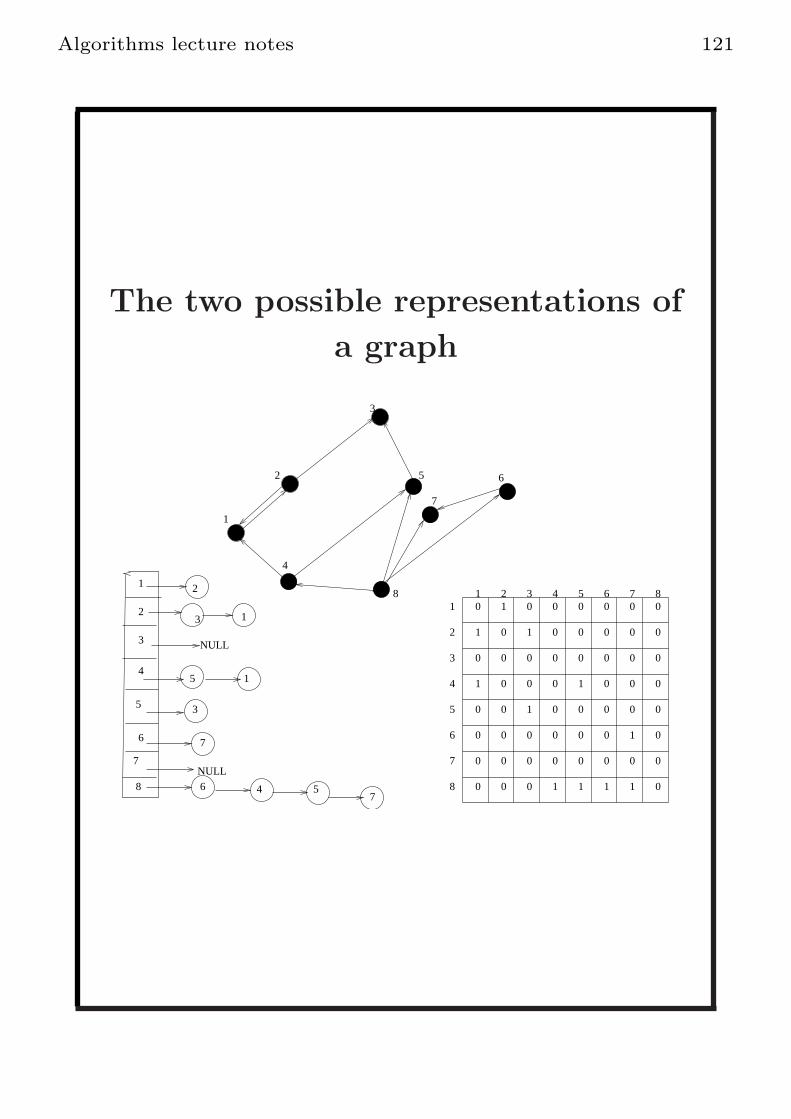
Say that the vertices are 1, 2, . . . , n.We build an n× n matrix and we put 1 in
A[i, j] if i 7→ j ∈ E and 0 otherwise.
Space n2.
Representing by linked lists
In A[i], A[i] points to the linked listt of
neighbors A[i] (the order could be any order
and depends on how the input was entered.).
Here the 0 of the Matrix are not represented
Algorithms lecture notes 121
The two possible representations of
a graph
1
2
3
4
5
8
6
1
2
3
4
5
6
7
8
2
3 1
NULL
5 1
3
7
NULL
6 4 57
1
2
3
4
5
6
7
8
0
0
0
0
0
0
0
0
1 2 3 4 5 6 7 81 0 0 0 0 0 0
1 0 0 0 0 0
0 0 0 0 0 0 0
1 0 0 1 0 0 0
0 0 1 0 0 0 0
0 0 0 0 0 1 0
0 0 0 0 0 0 0
0 0 0 1 1 1 1
1
7

Algorithms lecture notes 122
Computing the degrees of all
vertices
Say the graph is represented by a matrix.
1. For i = 1 to n do
(a) deg(i)← 0.
(b) For j = 1 to n do: if A[i, j] = 1 then
deg(i)← deg(i) + 1
2. Return D
The running time here is Θ(n2).

Algorithms lecture notes 123
Using linked list
We go to A[i] for every i, which is n.
In the directed case we spend degout(u) at U
and in total Θ(∑
u degout(u)) = Θ(m)
Total Θ(n+m) that may be much smaller than
n2.
For undirected graph the sum is 2m which is
insignificant.

Algorithms lecture notes 124
Relation between the number of
vertices n and the number of edges
m
If the graph is connected (one piece or finite
distance between any two vertices) we shall see
that m ≥ n− 1.
The maximum m can be is(
n2
)
< n2. Thus
m = O(n2).
For example (assuming no self loops or parallel
edges),√m = O(n).
The distance between a and b is the number
of edges in the shortest path between a, b
Do not say shortest distance. Distance is
already shortest.

Algorithms lecture notes 125
Distances
A B
C D E
X Y
THE DISTANCE BETWEEN A AND B IS 3
THE DISTANCE BETWEEN X AND A IS INFINITE.
THE DISTANCE BETWEEN X AND E IS 2

Algorithms lecture notes 126
A remark
Say that we add a collection of odd numbers.
Note that the sum is even if and only if
the amount of numbers is even.
In fact adding an odd number changes the
even/non-even status.
While adding even numbers leaves the status as
it was

Algorithms lecture notes 127
The number of odd degree vertices
We prove that the number of odd degree
vertices is always even.
A vertex can have either odd or even degree.
The two set VO of odd degree vertices and VE
of even degree vertices are disjoint.
So we can say that∑
v∈V deg(v) =∑
v∈VOdeg(v) +
∑
v∈VEdeg(v) = 2m
The last equality we have shown before.

Algorithms lecture notes 128
Continued
Thus∑
v∈Vo= 2m−∑
v∈VEdeg(v).
Note that∑
v∈VEdeg(v) is an even number.
This implies that∑
v∈Vo= 2m−∑
v∈VEdeg(v)
is even.
By the comment we made before, this implies
that |VO| is even

Algorithms lecture notes 129
Euler paths
This is a path that goes over every edge once.
It started because someone asked Euler about
the Seven Bridges of Knigsberg problem.
This was an area of water. Every vertex was
some ”island” and we put an edge between two
Islands if there is a bridge between them.
A person asked him if you can cross all the
bridges walking and go over all bridges exactly
once.
Walking means path.
Going over all the edges once: Euler path.

Algorithms lecture notes 130
An Euler path
e1 e2
e3
e4e5
e6
A
BC
D E
D E B C A B D C E
AN EULER PATH
e7e8
Algorithms lecture notes 131
Hotel California
An odd vertex can not be in the middle
(namely must start the path or end) of an
Euler path.
Like hotel California.
Say that deg(v) = 21 and we walk the path.
Each time we enter and leave v.
21 becomes 19, 17, 15, 13, 11 9, 7, 5, 3, 1.
At that moment v has degree 1 so after you
walk into v you are stuck.
You can check out any you like, but you can
never leave
So what happens if there are 4 or more odd
degree vertices?
No Euler path because only two vertices can
start and end the path

Algorithms lecture notes 132
The case of 2 and 0 vertices of odd
degree
If there are two odd degree vertices a, b we are
going to prove that there is an Euler path
that starts at a and ends at b.
If there are 0 vertices of odd degree we will
show that there exists an Euler cycle namely
an Euler path that starts and ends at the same
vertex.
Define the free degree of a vertex to be the
number of edges of v not yet traversed
We concentrate on the case of 0 odd degree
vertices. The case of 2 is similar. After you
enter and leave u the degree goes down by 2.
So all the time all free degrees are even.

Algorithms lecture notes 133
Expanding until you get stuck
Start at a vertex v. As long as the current
ending vertex u of the path has free degree
larger than 0 add an edge (u,w) that did not
appear yet, in the path at the end of the pat6h.
The path becomes larger by 1.
Getting stuck: If you get to a vertex of free
degree 0.
It seems that we ”failed” in this case to create
an Euler cycle.
But this is not true. The cycle can be made
larger and larger which means that at the end
its an Euler cycle

Algorithms lecture notes 134
An example of getting stuck
e1 e2
e3
e4e5
e6
A
BC
D E
E
e7e8
D E B C E

Algorithms lecture notes 135
Where can you get stuck?
If you started at v the free degree of every
vertex u but v is even after we cross u (namely
enter and leave).
You can not get stuck on a vertex with even
degree.
If you entered the free degree is even and at
least 2.
So you use one free edge to enter and one free
edge to leave and you do not get stuck.
Since the free degree of v is odd, you may get
stuck in v.
If you get stuck we have a cycle. It does not
matter where you started (in that you can
make the Euler path start at any vertex).

Algorithms lecture notes 136
We got stuck. The vertex we
started at is not important
1
2
3 4
5
6
89
10
11
12
7

Algorithms lecture notes 137
Extending a cycle
Because we closed a cycle and we got stuck and
the cycle does not contain ALL edges. There
are vertices of free degree larger than 0.
We start a new cycle at a vertex z of free degree
larger than 0 (hence at least 2) until we may
get stuck again. Again, we must get stuck at z.

Algorithms lecture notes 138
Treating the new cycle as a detour
Now we have two cycles.
The initial one.
And there is a cycle containing z. A second
cycle with new edges that did not appear before
Let the first cycle be C and the second C ′.
Create a new cycle: walk on C until z, and
then suspend walking on C.
Insert in the middle of the edges of C ′ until you
return to z.
Continue with the edges of C.

Algorithms lecture notes 139
Making the two cycles one
1
11
12
13
14
1516
17
18
19
2
34
5
6 7
8
9
10

Algorithms lecture notes 140
Our original example. The new
cycle starts and ends at B
.
e1 e2
e3
e4e5
e6
A
BC
D E
E
e7e8
D E B C Ee6 e5 e3 38
D E B A C D B C E

Algorithms lecture notes 141
Cycles upon cycles upon cycles
1
23
4
3
5
6
5
3
2
1

Algorithms lecture notes 142
And also:
WHO IS THE LEADER OF THE CLUB THA IS MADE FOR YOU AND ME?
Algorithms lecture notes 143
Directed graphs
An Euler cycle if and only if all the in degree of
vertices equals the out degree of the vertices.
Now, discuss the domino game.
The next picture will explain the domino rules
And the question is: can we put all the domino
pieces on a line so that all pieces are in, and
the configuration is a legal domino one.

Algorithms lecture notes 144
Playing domino
The peaces i, i for = 0 to 6 also exist.
THE DOMINO ROOLEES
P Q
P AND Q TAKE ALL NUMBERS BETWEEN 0 AND 6
2 3
3 4
4 4
4 2
28 PIECES.
A LEGAL: DOMINO SEQUENCE.

Algorithms lecture notes 145
It turns out that a legal Euler
alignment with all pieces is just an
Euler path in the graph below
DOPES THIS GRAPH HAVE AN EULER PATH
0 1
2
34
5
6

Algorithms lecture notes 146
All degrees are 8
Hence we do not have all pieces aligned in a
line. They are aligned in a circle.
How can we make a line out of them?

Algorithms lecture notes 147
The story of the Gordian Knot
No one was able to open a complex Knot
Alexander III of Macedon took a sword and cut
the knot. He must have been an Israeli.
He is also called Alexander the great.
The name of the hero of ”A clockwork Orange”
is Alexander De-Large.
How can we put the pieces on a line?

Algorithms lecture notes 148
The solution
Open the cycle and put the pieces in a line.
As simple as that.
We got a property that without Euler theory
we could never have known.
In every legal alignment of the pieces, the open
value at the start and the open value at the
end are equal.

Algorithms lecture notes 149
Directed acyclic graphs
Directed graph not containing directed cycles.
All paths are simple.
Extending paths in a DAG (Directed Acyclic
graph) shows two interesting things.
Say we start at u0 7→ u1 as a directed edge.
If there is an edge z1 7→ u0 we add it getting a
path z1 7→ u0 7→ u1
And z2 7→ z1 7→ u0 7→ u1.
Note that every z is a new vertex for otherwise
we got a cycle. This must finish. Hence we
have shown:
Remark: Every DAG has at least one vertex
of indegree 0.
The same argument shows that every DAG has
a vertex with out degree 0

Algorithms lecture notes 150
An example of a directed graph
with no directed cycles
A
B
C
D
E
F
G

Algorithms lecture notes 151
Topological sorting
Claim: in a DAG you have vertices of indegree
0 and outdegree 0.
Proof: extend a path until you cant, namely x1
the first vertex has no entering edges to new
vertices and the vertex and xk at the end does
not have out edges to new vertices.
Let P be path. There could not be an edge
from xp into x1, 1 < p as otherwise we get a
cycle. There could not be an edge from xk into
the path as this gives a cycle.
This means that x1 has indegree 0 and xk has
outdegree 0.
A topological sorting is arranging thee vertices
us u1, u2, . . . , un on a line so that every edge
that start at some vertex ui and end on uj has
i < j (all edges go right).
In general directed graph a cycle of size 3
implies that this is not possible.

Algorithms lecture notes 152
An algorithm to find a topological
ordering on a DAG
1. W ← V , G′ ← G.
2. While W 6= ∅ do:(a) recompute the in degrees in G′
(b) Let w be a vertex of indegree 0 in G′
(c) Output w as next in the order
(d) W ←W − w and G′ ← G− w
3. Return the ordering

Algorithms lecture notes 153
A DAG and one of the topological
orderings
A
B
C
D
E
F
G
A G F C B D E

Algorithms lecture notes 154
Why does it work
When adding the i consider a vertex j < i.
By definition after we remove 1, 2, . . . , j − 1
deg(j) = 0.
Which by definition means that vertices in
W = V − 1, 2, . . . , j − 1 do not have edges
into j.
This is a partial order. Edges go only to the
right. But some vertices can not be compared.
If we have a cycle of size 3 no matter the
ordering, one edge will go backward and so
there is no topological ordering

Algorithms lecture notes 155
The longest path on a DAG is a
polynomial question
In a DAG all paths are simple.
So to see if there is a paths of size k or more
can be done in polynomial time.
Try all vertices as start vertices of the path.
For v you go to the neighbors of v, and give
them distance 1, and go the the neighbors of
neighbors that did not get a distance yet and
give them distance 2. And so on. If the graph
is not exhausted before we get a path of length
k, it exists. This is because every new neighbor
did not appear before.
In general directed graphs this would have
produced cycles. Hence non simple paths hence
fails.
A famous NPC problem the longest path can
be solved in DAGS. In general directed graph it
does not work since the paths we find are not
simple.

Algorithms lecture notes 156
Shortest path on a DAG
When edges have weights, the length of a path
is the minimum sum of lengths among all
paths. In fact this path may have much more
edges than the case all edges have length 1.
Using the topological ordering gives fast
running time. The distances from s to all the
rest.
We have a number λ(v) for every v. Let
e = u 7→ v be an edge.
Definition:
To relax over the edge u 7→ v is to check if
λ(u) + ℓ(u, v) < λ(v) and if so, set
λ(v)← λ(u) + ℓ(u, v).

Algorithms lecture notes 157
Continued
Property 1: Take an exercise to prove by
induction that for the following algorithm if the
value of w is λ(w), there exists an s to w path
of length λ(w).
Note that we do not mind if edges have
negative distance (we need this for flow).
Because there are no cycles and so no negative
cycles
We can also find a distance with negative
weights if the source can not reach a negative
cycle or if there are no negative cycles at all.

Algorithms lecture notes 158
Shortest path from s algorithm
Algorithm(Short(G, s)
1. λ(s)← 0, and λ(u)←∞ for every u 6= s.
2. Find a topological sorting of G
3. Let the vertices be s = u1, u2, . . . , un and
assume without loss of generality that this
is a topological ordering.
4. For i = 1 to n− 1, relax all the edges going
out of ui
5. Return λ(uini=1

Algorithms lecture notes 159
Example
Relaxing S 7→ T , S 7→ X
Relaxing T 7→ Y and T 7→ Z.
R5
S
0
T X Y Z
6
infty
3
1
4 6
2 7 −1 −2
3
5R
2
16
T XY Z
4
6
5
6
S T
7
72
6
Y
Z
4
66
−1 −2
−1 −2
Lambda(x)=6
Lambda(T)=2
x
Lambda(Y)=6
Lambda(z)=8
S
S
Lambda(X)=9

Algorithms lecture notes 160
Example
Relaxing X 7→ Y , X 7→ Z
Relaxing Y 7→ T
R5
S
0
T X Y Z
6
infty
3
1
4 6
2 7 −1 −2
3
5R
2
16
T XY Z
4
6
5
6
S T
7
72
6
Y
Z
4
66
−1 −2
−1 −2x
Lambda(Y)=6
Lambda(Y)= 5
Lambda(z)= 3
No Change.
Lambda(Z)= 8
Lambda(Z)=7
Lambda(X)=6
Lambda(X)=6
Lambda(Z)=6
Lambda(Y)= 5

Algorithms lecture notes 161
Running time
Go over every vertex and its out degree.
Sum of outdegree is m (the number of edges.
So O(m+ n).
But why is it correct?
We need to prove this by induction.
The induction is on the iteration.
Since the iterations are a collection of integers
First namely 1, second, namely 2, etc.
The base case is S. Clearly gets 0 the right
value.

Algorithms lecture notes 162
Consider iteration i+ 1
It did relax to all the edges of the first i
vertices.
Let u be the i+ 1 vertex.
A path from s must have a one but last vertex
v.
So that dist(s, u) = dist(s, v) + ℓ(u, v)
But v is a vertex that lies in a shortest path
between s and v. So it was relaxed.
By induction hypothesis λ(v) = dist(s, v).
So by definition, since
λ ≤ dist(s, u) + ℓ(e) = dist(s, u)
But also λ(s, v) ≥ dist(s, v) by Property 1.
Hence λ(u) = dist(s, u).

Algorithms lecture notes 163
Finding shortest paths in general
directed graphs
The unweighted case. Special case.
If all distances are 1 then distance 1 is your
neighbors.
Distance 2 are the neighbors of neighbors.
This is tricky, a neighbor of a neighbor can be
also a direct neighbor
So when v gets a value, we cant allow it to get
a value again.
Later we shall see that for positive weights, the
value of the distance of v changes many times.

Algorithms lecture notes 164
If a vertex already has a value, do
not change it
Distances from A. B,C get distance 1. When
we go to B, be careful not to give value 2 to C.
New values are given only to vertices of infinite
distance from A.
A
BC
C IS A NEIGHBOR OF A BUT ALSO OF B. RISK THAT C WILL GET 2.

Algorithms lecture notes 165
The BFS algorithm
1. Q← s
2. For all v ∈ V \ s dist(s, v)←∞.
dist(s, s)← 0.
3. While Q 6= ∅ do(a) v ← Delete(Q).
(b) u← N(v)
(c) While u 6= Null do:
i. If dist(s, u) =∞ then
A. dist(s, u)← dist(s, v) + 1
B. Add(Q, u)
ii. u← next(u)
4. Output the distance vector.

Algorithms lecture notes 166
A run of BFS
A
B
CD
E F G H
X Y Z
P Q R S
M
A C D B
B
C H G D
D
E Y X
F
G Z
H
X P
Y R Q
Z S
P G
Q F M
R
S D
M
A
C
D
B
11 1
1 23
45
2 2
E F
G
H
2
2
3 3
Z
X
Y
E
F
3

Algorithms lecture notes 167
A run of BFS, continued
A
B
CD
E F G H
X Y Z
P Q R S
M
A C D B
B
C H G D
D
E Y X
F
G Z
H
X P
Y R Q
Z S
P G
Q F M
R
S D
M
11 1
1 23
45
2 2
E F
2
2
3 3 3
Z
X
Y
4
S
R
Q
P
4 4
6 7
5
M
Algorithms lecture notes 168
Correctness of BFS
We prove: All the vertices of layer i (namely, at
distance i from s) enter the queue before all the
vertices of layer i+ 1.
If this is true it is clear that BFS is correct.
A problem can be established if a neighbor of v
at level i+ 1 enters the Queue before a
neighbor of v in level i− 1 and thus v gets the
wrong distance: i+ 2.

Algorithms lecture notes 169
Proof by induction
The induction on the iteration starts with
i = 0. This is the vertex s and the claim is
clear by the algorithm.
Assume the claim hold for i. We shall see that
all the i+ 1 layer vertices, enter the queue
before the i+ 2 vertices.
Let u be a vertex in layer i+ 1, and let w be a
vertex of layer i+ 2.

Algorithms lecture notes 170
Continued
By definition, there are, respectively, vertices
u1 and w1 in layers i and i+ 1, so that
(u1, u), (w1, w) ∈ E.
Note that by the induction hypothesis, u1 will
enter the queue before w1 (or any other vertex
in layer i+ 1, that has w as a neighbor).
When we scan u1, (maybe before) u will enter
the queue. This implies that u enters the queue
before w (as no w1 vertex with (w1, w) ∈ E can
have been scanned yet, by the induction
hypothesis). The claim follows

Algorithms lecture notes 171
Running time of BFS
The algorithm goes over all vertices.
If we do this in linked list implementation, for
every vertex u in the worst case it goes over
all the edges of u once.
An edge of u is not traversed twice because u
can no longer help his neighbors.
Since∑
v∈V degout(v) = m the running time is
linear.
Namely Θ(n+m).

Algorithms lecture notes 172
The running time on a connected
undirected graph
Here m ≥ n− 1.
Thus n ≤ 2m.
Thus n = O(m).
Thus for a connected graph the running time is
Θ(n) in the worst case.

Algorithms lecture notes 173
An algorithm is an idea: Strongly
connected graphs
Strongly connected graph: All distances
between any two vertices, finite.
A simple algorithm:
Run BFS on all v and check that no vertex in
V − v has infinite distance. Θ(n2).
Alternative:
Claim: A graph is strongly connected if and
only if there exists a vertex v so that V − v has
both finite distances from v and to v.
Why? If strongly connected the above is clear.
Also, if a wants to reach b a takes the path to v
and then the path from v to b.
Two BFS runs. One with edges reversed to see
that all V − v vertices have a path to v. O(n)

Algorithms lecture notes 174
Finding shortest path from s to
V \ S when there are non uniform
cost over edges: The algorithm of
Dijkstra
We assume a data structure that supports
insert and delete min in time O(log n) each.
Recall what relaxing is.
Let λ(v) be the shortest path we found so far
from s to v.
Recall: To relax over an edge e = u 7→ v is
to check if u can help them get a lower path
from s.
Namely, if λ(u) + ℓ(u, v) < λ(v), set
λ(v) = λ(u) + ℓ((u, v)).
We just found a shortest path for v, namely the
path of length λ(u) from s to u and the direct
edge u 7→ v.

Algorithms lecture notes 175
A priority QUEUE
Aranges items with real keys so that we can do
fast the following operations.
1) Insert(S, x)
2) Delete−Min(S)
3) Decrease−Key(S, x, y). The key is unique.
So reduce the x into y.
Fibonacci Heaps (more or less) can do 1,2, in
O(log n) and Decrease−Key in O(1)

Algorithms lecture notes 176
The algorithm of Dijkstra
1. For all v 6= s set λ(v) =∞
2. Build a priority Queue of V with respect to
λ.
3. While S 6= ∅ do:(a) u← Delete−Min(S)
(b) For any neighbor v of u relax(u 7→ v).
/* This is a dcrease key operatio */
4. Return λ(v).

Algorithms lecture notes 177
A run of the algorithm of Dijkstra
2
3
8
10
1
3
A
D
T
INFTY INFTY
0
B
2
2 10
INFTY
T INFTY
INFTY
A
B
A
2
3
INFTY
6
8
1
3
3
5C
102
6
8
1
3
6
6
5
6
6
6
INFTY 12
6
B
INFTY
INFTY
EC
INFTY
12
5
11
INFTY
INFTY
T
2B
6
INFTY
1
1
1
E
E
13

Algorithms lecture notes 178
A run of the algorithm of Dijkstra
Continued
2
3
8
10
1
3
A
B
C
D
E
T
INFTY INFTY
INFTY INFTY
INFTY
0
B
2
2
INFTY
D10
INFTY
T
INFTY
INFTY
INFTY
A
B
A
2
3
INFTY
6
6 8
1
3
3
5C
10 12
2
6
8
1
3
2
12
11
13
65
6
6
5
65
6
6
INFTY 1211
13
D12
6
B
C
B
12
INFTY 13
12
12
INFTY
INFTY
11
14
114
13
1
1

Algorithms lecture notes 179
A basic property of shortest path
Say that P is a shortest path from s to t.
Then we claim:
Claim 1: If a and b belong to the shortest path
P from s to u, the part of the path between a
and b is a shortest path as well.
13S
P
TA B
12
STA B
Indeed, if it was not a shortest path, we could
replace the subpath of a to b by a shorter one
and thus P is not a shortest path,
contradiction.

Algorithms lecture notes 180
The vertices x and y
Consider a shortest path P from s to u.
As s is to the left of u and was chosen, the
concept of the rightmost vertex that is not
u that was chosen is well defined.
Let x be such a vertex. Let y be the vertex
right after x (so not chosen).
dist(s, x) = λ(x) by the induction hypothesis.
But by the property of shortest paths
distP (s, y) = dist(s, y).
Remark: our main goal is to show that
dist(s, y) = λ(y). If all vertices to the left of u
are chosen this follows from the induction
hypothesis.

Algorithms lecture notes 181
illustration
S X
HE RIGHTMOST TO BE CHOSEN
Y
BY INDUCTYION
UP
LAMBDA(X)= DIST(S,X)
BY SHORTEST PATH PRINCIPALDIST(S,Y)=DIST(S,Y)P
Algorithms lecture notes 182
A property that always holds in all
shortest path algorithms
PROPERTY 1: If the value of z is λ(z) then
there is a path from s to z of length λ(z)
In fact λ gets smaller and smaller (except for
BFS) until its the right distance.
Prove this property by induction as an exercise.

Algorithms lecture notes 183
Showing that dist(s, y) = λ(y)
Equation 1: dist(s, y) = λ(y)
PROOF
Since the distance on P from s to y is the
distance from s to y:
distP (s, x) + ℓ((y, x)) = distP (s, y) = dist(s, y)
Because of that and Property 1,
distP (s, y) = dist(s, y) ≤ λ(y).

Algorithms lecture notes 184
It can not be that λ(y) > dist(s, y)
Note that x is an already chosen vertex,
Hence the edges x 7→ y was already relaxed.
Thus λ(y) ≤ λ(x) + ℓ(x 7→ y) =
dist(s, x) + ℓ(x 7→ y) = dist(s, y).
The equality λ(x) = dist(s, x) follows from the
induction htpothesis.
This proves Equation 1 END PROOF

Algorithms lecture notes 185
Ending the proof
By definition u was the last chosen vertex.
This means that λ(u) ≤ λ(y) since we pick u
with minimum λ value.
We show that when a vertex u is chosen
λ(u) = dist(s, u).
Since all vertices are chosen, the distances are
correct.

Algorithms lecture notes 186
Proof continued
For the sake of contradiction assume
λ(u) 6= dist(s, u). Note that λ(u) < dist(s, u)
cant happen because of PROPERTY 1.
We are left with one possibility only
λ(u) > dist(s, u)

Algorithms lecture notes 187
Proof continued
Getting a contradiction
λ(u) ≤ λ(y) as u was chosen before y
= dist(s, y) By Equation 1
< dist(s, u) y is closer to s than u
≤ λ(u) Because of EQUATION 1
We got λ(u) < λ(u), contradiction.

Algorithms lecture notes 188
Running time
We have n time Delete-Min and a Priority
QUEUE can do it in O(log n) for a total of
O(n logn).
The rest is relaxing. Note that there is at most
one relaxing per edge because if we do relaxing
for the neighbors of u, u was selected,
λ(u) = dist(s, u) and thus there will be no
more relaxing for any edge of u.
The relaxing is a Decrease-Key operation.
Fibonacci-Heaps can do Decrease-Key in O(1).
Running time Θ(n logn) + Θ(m).
If m ≥ n logn the time is linear namely
O(m+ n).
But the time is not linear.
This is an open question (as far as I know).

Algorithms lecture notes 189
Finding the minimum distances
from s when there are negative
values
Important for flow, later.
We must detect a negative cycle which can
make distance −∞.
The Bellman Ford algorithm
1. Arrange the edges of the graph as
e1, e2, . . . , em.
2. For every v 6= s λ(v)←∞.
3. For i = 1 to n− 1 do
(a) For e = e1 to em relax(e)
4. Return λ(v)

Algorithms lecture notes 190
Correctness
Assume no negative cycles.
Claim: any relaxation keeps the property that
λ(v) ≥ dist(s, v)
Because λ(v) is the length of some path to v.
Claim: If no negative cycles, after i rounds,
λ(u) is the shortest path from s to u among all
paths with at most i edges.
Proof, by induction. Consider iteration i+ 1
and a vertex v. For all u 7→ v ∈ E, e = u 7→ v
was relaxed. Let us say that relax(x, v) gave
the shortest value. By the induction
hypothesis, λ(s, x) is at the moment the
shortest path from s to x among paths with i
edges.
By definition: the shortest path from s to v
with i+ 1 is the shortest path to some x among
paths of length i, plus the edge ℓ(x, v).
Algorithms lecture notes 191
Correctness of Bellman Ford
The algorithm is correct, assuming
no negative cycles
Proof: By the claim above and since a (simple)
path contains at most n− 1 edges, the claim
follows.
Detecting a negative cycle
After the algorithm is done, we look for u 7→ v
so that dist(s, v) > λ(u) + ℓ(u 7→ v)
If there were no negative cycles, the distances
were correct and so by the definition of
distance, dist(s, v) ≤ dist(s, u) + ℓ(u, v) as
u 7→ v was relaxed.
The fact that this does not hold, means a
negative cycle. If there is a negative cycle we
can always relax.
So an inequality as above will happen Running
time O(n ·m).

Algorithms lecture notes 192
Free (namely non rooted) trees
Definition: a graph is a tree if it is connected
and has no cycles.
STAR PATH
Algorithms lecture notes 193
A basic property
In a tree:
1) There is a unique path between two vertices,
because its connected and two different paths
give a cycle.
A leaf is a vertex of degree 1.
2) We shall show that there are always at least
2 leaves in a tree. By growing a path.
Start with (a, b) (any edge). Let x, y be the
endpoints of the path P .
If x has a path outside to some z 6∈ P extend P
by z. The same goes for y. When we cant do it
anymore x, y are leaves: no edge to a vertex
outside P and no additional edge inside P as
this gives a cycle.

Algorithms lecture notes 194
Example
A
B
C
DE

Algorithms lecture notes 195
The number of edges in a tree
Noah’s Ark.
In iteration marry a leaf and a its vertex.
Until one vertex remains.
Because its one to one an onto (disjoint pairs)
we get that besides the last vertex left there
are the same number of vertices and edges.
So m = n− 1.

Algorithms lecture notes 196
By induction
We will prove by induction that a tree of n
vertices.
When n = 1 the number of edges is 0 (a self
loop is a cycle).
Say that its true up to n and let T be a tree of
n+ 1 vertices. Removing a leaf ℓ makes the
resulting graph still a tree, and by induction
this tree has n vertices and n− 1 leaves
After adding the leaf back we get n+ 1 vertices
and n edges and the proof is finished.

Algorithms lecture notes 197
The minimum connectivity
property of a tree
A spanning tree is a tree containing all vertices.
If you add an edge to a tree say (a, b) to a
spanning tree then a unique cycle is closed
because there is already a path from a to b.
If you remove any edge e from a tree, we get
two trees and a disconnected graph. It cant be
that T − e is still a spanning tree, because in
such a case e belonged to a cycle.
Now say that we want to lay train tracks so
that all important cities in the country can get
to all other important cities by a train

Algorithms lecture notes 198
The research department
Produce a graph.
The vertices will be the big cities.
There will be edges between two cities if it is
possible to lay train track between the two
cities. Some time its impossible (”Blazing
Saddles”) because there is a lake or the likes
between the two cities.
Each edge has a cost that says how much
money will it take to lay a train truck between
the two cities.
We want to choose a collection of edges that
connect every two cities (namely the graph is
connected) and among all such graphs, choose
one with minimum cost.

Algorithms lecture notes 199
A
BC
D
EF
GH
I
JK
1
11
1
1 12
33
2
2
4 51
1
A
B
H
1
1
1
1
2
J2
1
I
K
F
1
6
D
1
3
J
2
C
1
G

Algorithms lecture notes 200
The minimum spanning tree
problem
A subgraph that connects in minimum cost
every two vertices (cities) will be a spanning
tree.
It must be connected by definition.
But if we have a cycle, we can clearly remove
an edge from the cycle, keep connectivity and
get a lower cost.
Thus we need to choose a spanning tree
T (V,E′) and among all spanning trees the one
whose edge wights sum is minimum.

Algorithms lecture notes 201
The distance of a vertex from a
tree
Given a non spanning tree T a vertex u can
have many neighbors in T .
Say that the one with least price is near(T, v)
We use costs as distance.
Let u← near(T, v)
Define dist(v, u) = c(u, v).
We are going to present a greedy algorithm that
add leaves to a tree, and each time adds the
closest leaf.

Algorithms lecture notes 202
The Prim algorithm
Let the vertices be 1, 2, . . . , n so that some i, j
have an edge and the cost is c(i, j).
1. E′ ← ∅.
2. T ← 1
3. While T is not a spanning tree do:
(a) For every v 6∈ T compute dist(v, T )
(b) Let j be the vertex with minimum
distance from the tree of cost dist(j, T )
(c) Say that j achieves the minimum with
edge e.
(d) E′ ← E′ ∪ e.
4. Output(E′).

Algorithms lecture notes 203
A run of Prime
. The numbers give the order by which edges
are added (do not confuse with weights).
A
B
C
D
F
G
H
X
ZR
1
1
1
2
3
2
2
2
4
3 2
2
2
1
A
B1
2
D
3
3
C
3
4
5
G
67
8
X
H
Z
F
10
R
G 2
THE ORDER BY WHICH THE EDGES ARE ADDED.

Algorithms lecture notes 204
Correctness for Prim
1. Extendible set E′: A set so that there exist
some optimum collection of edges OPT so
that E′ ⊆ OPT .
2. In such a case OPT is called a witness for
E′.
3. Let E′ be the set of edges of the current
Prim tree. By the induction hypothesis,
there is some OPT1 that E′ ⊆ OPT1.
We are adding an edge e to E′. Our problem is
that it may be that e /∈ OPT1, so
E′ ∪ e 6⊆ OPT1.
So wee need a new witness OPT2. This should
be a MINIMUM SPANNING TREE
THAT CONTAINS BOTH E′ and e.

Algorithms lecture notes 205
The idea of the proof of correctness
The idea how to get to OPT2 from OPT1.
Add e to OPT1. The resulting structure is not
a tree, so cant be a witness.
Since OPT1 is a spanning tree, OPT1 + e has
a unique cycle C.
Find an edge e′ to remove from OPT1 ∪ e sothat:
1. OPT2 = (OPT1 ∪ e) \ e′.
2. OPT2 is a tree.
3. c(e) = c(e′)
This edge e′ MUST BE ON THE CYCLE
C AS WELL as otherwise you dont get that
OPT2 is a tree.

Algorithms lecture notes 206
Making sure c(e) = c(e′)
The first edge e = (u, v) in the cycle goes
inside T .
Namely u 6∈ T and v ∈ T .
The cycle also ends outside T . Thus the cycle
must have another touching edge different than
e (as otherwise we stay in T ).
By the definition of e, c(e) ≤ c(e′).
Since both trees are minimum cost spanning
trees c(e) = c(e′)

Algorithms lecture notes 207
1
1
1
2
2
2
4
5
1
1
a
c
d
f
g
1
x
x
a
d
g
C
e’
x
a
d
f
g
OPT1
OPT2
ey
THE EDGE e
fcc
y
y
ANOTHER TOUCHING EDGE
e
d y
f
a
x
c
g

Algorithms lecture notes 208
In summary
OPT2 is OPT1 with the difference that we add
e and remove some e′.
But since c(e) = c(e′) they have the same cost.
So OPT2 is also a minimum spanning tree.
So we found a witness to E′ + e.At the end |E′| = n− 1. And is contained in a
minimum spanning tree.
But since a spanning tree also has n− 1 edges,
Clearly G(V,E′) is a minimum spanning tree

Algorithms lecture notes 209
The algorithm of Kruskal;
1. Sol← ∅
2. Sort all edges in non decreasing weights
3. Let the sorted edges be e1, e2, . . . , em
4. For = 1 to m, if Sol + ei has a cycle,
discard ei
5. Else Solu← Sol ∪ ei

Algorithms lecture notes 210
A run of the Kruskal algorithm
A
B
C
D
F
G
H
X
ZR
1
1
1
2
3
2
2
2
4
3 2
2
2
1
A
B
D
3
3
C
35
G
X
H
Z
F
R
THE ORDER BY WHICH THE EDGES ARE ADDED.
12
4
6
7
H
8
9
10

Algorithms lecture notes 211
Correctness
We have to show a witness OPT that contained
Sol even after we add the next edge e.
The base is trivial correct since Sol = ∅.Say that the witness now is Sol ⊆ OPT1.
Say that e 6∈ OPT1.
Add e to OPT1. A unique cycle is closed.
At the moment e is added it connects together
two connected components C1 and C2.
Without e, therefore, there is a path from C1
to C2.
Thus there is another edge going with one end
point in C1 and one endpoint outside C1.
Let this edge be e′.
By definition w(e) ≤ w(e′).
Which means w(e) = w(e′).
Thus OPT1 + e− e′ is a new witness

Algorithms lecture notes 212
Running time: Union-Find
We maintain a forest
Once an edge e = (a, b) arrives we need to
know (fast if possible) if a and b are in the
same connected component.
If so we skip a, b.
Else we need a way to do Union: represent the
union of the two connected components as one.
This data structures is called Union Find

Algorithms lecture notes 213
Union Find
The edges start as sets of size 1.
Then we unite two connected components to
one.
Method: Every connected component will be
represented by a linked list of its vertices.
Uniting two connected components S1, S2 is
the operation Union(S1, S2). It means that we
just added an edge from S1 to S2.
The connected component needs a name:
Show me to your leader.
Every vertex has a second pointer L(x) called a
leader pointer to the first vertex in the linked
list (the leader).
We also need to implement the operation
Same(a, b) which asks: the next edge is (a, b).
Do a and b lie in the same connected
component?
This is implemented by comparing L(a) and
L(b). Requires O(1) time.

Algorithms lecture notes 214
Representation
x y w z q p

Algorithms lecture notes 215
A union
x y w z q p
a bc
x y w z q p a b c
CHANGE THE LEADER POINTERS OF THE SMALLER SET TO THE LEADER OF THE LARGER SET

Algorithms lecture notes 216
The total running time
Say we have m finds and Same(x, y). Same is
executed by taking the leader pointers and
comparing them. O(1) operation. Thus Θ(m)
for all Same and Find
The number of unions is at most n− 1.
The time spent on unions is the number of
times each element gets a new leader.
Basic property: if you get a new leader the size
of your list at least doubles.
Thus no item has more than log2 n changes.
So the total number of operations in union
requires O(n · log n).

Algorithms lecture notes 217
An implementation of Union Find
via trees
We maintain trees.
To check the leader of the tree requires the
height of the tree.
A new item is added as a leaf.
When we do Find all the vertices in the path
become children of the root.

Algorithms lecture notes 218
How to improve the find tree
A
B
C
D
E
A
C
D E
FIND(E)
B

Algorithms lecture notes 219
Running time
Union: the tree with smaller (or equal) height
becomes the child of the root of the other tree.
O(1) operations.
The improvement seen in the figure is vital.
It can be seen by a complex analysis that the
total number of operations is n · α(n) with α(n)
the inverse Ackerman function.
This was, I think, the Ph D. thesis of Tarjan.
The inverse Ackerman function when applies
on 2300 (more than the number of atoms in the
known universe) is 4.
It is not linear as α(n) goes to infinite when n
does.
But for all practical purposes, its at most 4.
Tarjan showed an example when the n · α(n) isindeed the running time, hence its tight.
I also showed it. In the homework

Algorithms lecture notes 220
Maximum flow in a networks
The input for the maximum flow problem is a
directed graph G(V,E) with capacity c(e) > 0
for every e ∈ E and two distinguished nodes: a
source s and a target t
We will assume no edge enters s and no edge
leaves t
A legal flow is a flow function f : E 7→ R+ that
obeys the following restrictions:
1. Capacity constraint: f(e) ≤ c(e) for every
e ∈ E
2. Flow conservation constraint: for every
v 6= s, v 6= t,∑
e∈in(v)
f(e) =∑
e∈out(v)
f(e).

Algorithms lecture notes 221
The goal in a maximum flow
problem
The scenario described is that some
commodities (could be fluids or electricity or
automobiles) from s to t
The middle vertices do not create nor waste
flow.
Hence the goal is to maximize:
∑
e∈in(t)
f(e).

Algorithms lecture notes 222
Example
3
8
1
5
1
6
1,
2,
2
1,
1,
91,
10
2,
1,
2,
a
b c
d
st

Algorithms lecture notes 223
A basic flow property
The flow can be measured at every cut.
A cut (S, S) is a partition of V into V = S ∪ S,
S ∩ S = ∅ so that s ∈ S and t ∈ S.
The flow along the cut is:
∑
e∈e(S,S)
f(e)−∑
e∈e(S,S)
f(e)
This is called the net flow along the cut

Algorithms lecture notes 224
Example
3
8
1
5
1
6
1,
2,
2
1,
1,
91,
10
2,
1,
2,
a
b c
d
st
s
d
b
t
a
c
1
2
1
1
1+2+1−1−1=3

Algorithms lecture notes 225
All net flows are equal
S
v
x w
z
y
y
xz
w
Z−Y=X−W
Z+W=X+Y

Algorithms lecture notes 226
The net flow does not depend on
the cut
Since moving a single vertex from left to right
does not change the flow (and similarly, moving
a vertex from right to left does not change the
flow) by moving vertices (except for s, t)
around we can get any proper partition.
Thus, for any S, S,
f(S) =∑
e∈S 7→S −∑
e∈S 7→S = |f |For example, the value of the flow also equals
the amount of flow that goes out of s

Algorithms lecture notes 227
The capacity of a cut
Given a cut S, S, s ∈ S, and t ∈ S the capacity
of the cut is defined by:
c(S)∑
e∈S 7→S
c(e).
Remarks:
• The capacity of a cut depends on the
graph and the partition. In does not
depend on any specific flow
• In the capacity of a cut (unlike net flow)
we only take edges that go from S to S

Algorithms lecture notes 228
Every cut capacity bounds any
flow value
Claim 1. For every cut S, S, and legal flow f ,
|f | ≤ c(S).
Proof.
|f | =∑
e∈e(S,S)
f(e)−∑
e∈e(S,S)
f(e)
≤∑
e∈e(S,S)
f(e) ≤∑
e∈e(S,S)
c(e)
= c(S)

Algorithms lecture notes 229
The world of the dwarfs and giants
Every cut capacity bounds from above any flow
value. If there are f∗ and S∗ so that
|f∗| = c(S∗) then the flow is maximum and the
capacity is minimum

Algorithms lecture notes 230
c(S)
c(S’)
ff’
f’’f * S *

Algorithms lecture notes 231
The min-cut max-flow theorem
We are going to prove:
Theorem 1. For every network, the min-cut
equals the max-flow
This was proved by Ford and Fulkerson in
1955. The proof used the first ever algorithm
for finding the max-flow.
The min-cut is also discovered

Algorithms lecture notes 232
How do we compute a max-flow?
Improvements: the simple possibility:
s
a
b
t
M
M
M
1
M
+1
+1
+1
M
1,M
1,1
1,M
0,M

Algorithms lecture notes 233
Some time flow reduction on edges
help
s
a
b
t
M
M
M
1
1,
1,
1, M
+1
−1
+1

Algorithms lecture notes 234
The residual graph
s
a
b
t
M
M
M
1
1,
1,
1, M
M M−11
M−1
1M
1,M
1,M
1,M1,M
0,1

Algorithms lecture notes 235
The residual graph: definition
If an edge e = (u, v) has capacity c and flow f
then:
1. It has an edge in the same direction of e iff
f < c
2. It has an edge in the reverse direction of e
(this means the edge (v, u)) if and only if
f > 0
3. If f < c then the edge in the same
direction as e has capacity c− f .
4. If f > 0 the edge in the reverse direction to
e has capacity f .

Algorithms lecture notes 236
Intuition
Idea: we are splitting the edges into original
and reverse edges.
Original edges: how much can we increase f?
No more than c− f .
Reverse edges: how much can we decrease f?
By no more than f .
Instead of going in a “no entry” street (on
edges in the reverse direction) we simply add
the anti-parallel edge

Algorithms lecture notes 237
s to t paths in R(G, f)
Claim: if there is an s to t path in P in
R(G, f) we can increase f .
The idea: let
d1 = mine that is an original edge in P
c(e)− f(e),
d1 = mine that is a reverse edge in P
f(e),
d = mind1, d2.
It must be that d > 0 because there is a path in
R(G, f) between s and t.
Add d units of flow to every original edge in P
and subtract d flow units from every reverse
edge

Algorithms lecture notes 238
The flow is still legal
+d +d
+d −d
−d −d
−d +d

Algorithms lecture notes 239
The flow has increased
Since the path is from s to t it starts with an
original edge (s, x).
The flow along (s, x) was increased by d.
Thus the value of the flow is larger: the value
of the flow can be measured at s.
But: if no s to t path exists in R(G, f) does
this mean that f is a maximum flow? Yes!

Algorithms lecture notes 240
Proof of the min-cut max-flow
theorem
Consider all vertices that are reachable in
R(G, f) from s:
a
b
c
s
f=c
f=c
f=0
f=0

Algorithms lecture notes 241
The cut that equals the flow
The vertex s with all the other vertices it can
reach in R(G, f) is a subset S ⊆ V
The subset S contains s but not t
All edges that go from S to S are saturated
All edges that go from S to S have flow zero
Therefore c(S, S) = |f |Thus, the flow is maximum and the cut is
minimum
We still need to show an algorithm that finds a
flow with no augmenting paths in polynomial
in the input time
Algorithms lecture notes 242
The Ford and Fulkerson algorithm
Find a directed path between s and t in
R(G, f). How? See later (BFS).
Augment the flow along the path by the
bottleneck.
Iterate.
The following example shows that this
algorithm can have bad running time:
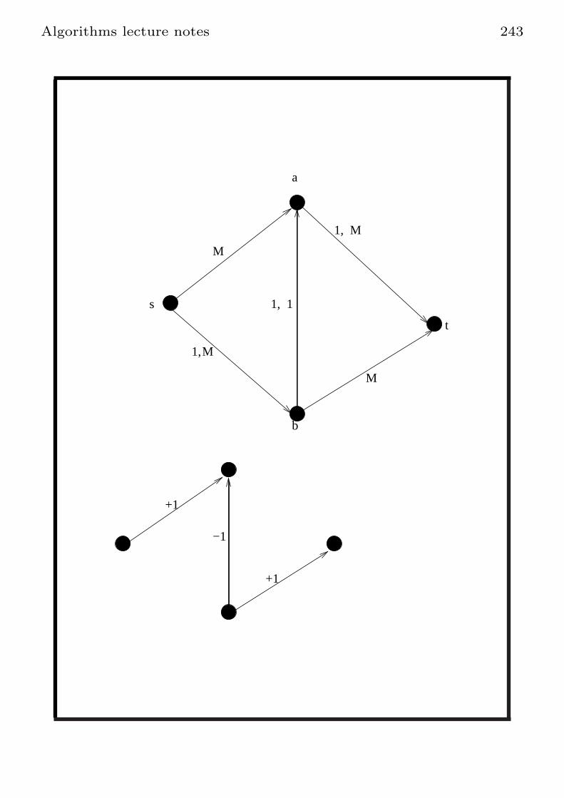
Algorithms lecture notes 243
s
a
b
t
M
M
M
1
1,
1,
1, M
+1
−1
+1

Algorithms lecture notes 244
The running time of FF and better
algorithms
The above example shows the running time can
be O(M).
Thus not polynomial in the size of the input
Two choices give polynomial time algorithms:
1. Select the least number of edges paths
when you augment (later we see how to
find such path)
2. Select the highest bottleneck path

Algorithms lecture notes 245
The Edmonds-Karp algorithm
Select BFS paths. Requires O(|E|).Claim: The distance in R(G, f) from s to x can
never decrease
Try to prove it at home. Provide proof later
Claim: The number of augmenting paths is
O(|E| · |V |)Proof: the distance between s and t can be
only 1 or 2, and so on up to |V | − 1.
How much time can the distance stay at k?
Claim: at most |E| augmenting paths can the
distance stay at k.
If we prove it we get O(|E| · |V |) augmentations
for O(|E|2|V |) running time

Algorithms lecture notes 246
Proof
A single augmentation reverses an edge
This edge can no longer serve in any shortest
path
d=10
d=9
d>=10
d=9
Therefore after O(|E|) augmenting paths there
is no length k path from s to t

Algorithms lecture notes 247
The bottleneck algorithm
Let R be the difference between the maximum
flow and the flow at the moment.
Claim: there is always a single path that
augments the flow by at least R/m for m = |E|.Before we prove it, let us see that this gives:
Claim: the bottleneck algorithm runs in
O (m · (log n+ logM)) time with M the
maximum capacity. Note: this is a polynomial
in the input time.

Algorithms lecture notes 248
Proof
Let f be the maximum flow value.
After the next augmentation,
Ri+1 = R
(
1− 1
m
)
.
Therefore after m · ln f augmentations:
Ri+1 ≤ f ·(
1− 1
m
)m·ln f
≤ 1.
We show this by noting that(
1− 1
m
)m
≤ 1
e.
So
f
(
1− 1
m
)m ln f
= f
((
1− 1
m
)m)ln f
≤ f ·(
1
e
)ln f
= 1

Algorithms lecture notes 249
Flow decomposition
The path claim: Given some flow f with value
|f | = x we show that we can select an s to t
path and a number 0 < d ≤ x so that:
: There exists a path P from s to t in G and
all the edges on the path carry at least d
units of flow
At least one edge in P carries d units of flow
exactly
If we can do that, we get the bottleneck claim

Algorithms lecture notes 250
The path claim implies the
bottleneck claim
Find P as promised in the path claim
Zero the flow on P
Iterate.
The process defines at most m paths because
for every P chosen the flow of at least one edge
is zeroed.
Conclusion: the reverse augmentation shows
that we may augment the flow to maximum in
at most m paths (always!).
Let |f | be the maximum flow and R the current
one. By averaging, at least one of the paths
carries (|f | −R)/m flow units or more
Remark: there are m paths that ONLY
INCREASES FLOW ALONG EDGES.

Algorithms lecture notes 251
The path claim
Start with |f |. Let e1 = (v, t) be an edge
entering t. Decrease the flow on this edge by 1.
There most be an edge entering v with
positive flow. Choose e2 = (u, v), f(e2) > 0 and
decrease the flow on e2 by 1.
There must be still flow entering u. Select e3
entering u and reduce the flow along e3 by 1,
etc.
A problem that may happen is the formation of
cycles

Algorithms lecture notes 252
A cycle
t

Algorithms lecture notes 253
Proof, continued
But cycles can be discarded and the process
can continue.
Until we get to s.
We found a path from s to t and define d to be
the least flow on this path.
Thus the path claim and the decomposition
claim both hold.
Question: why do we not get O(|E|2) time
algorithm?

Algorithms lecture notes 254
Maximum independent sets in
bipartite graphs
Given a graph G(V,E), a set W ⊆ V is an
independent set if there are no edges internal to
W .
A graph is bipartite if V can be split into two
independent sets V = V1 ∪ V2 and V1 ∩ V2 = ∅Let G(V1, V2, E) be a bipartite graph.
We show how to find a maximum independent
set in G.

Algorithms lecture notes 255
The flow network
Form the following flow network: direct the
edges of E from V1 to V2.
Add a source s and a directed edge from s to
each v1 ∈ V1 with capacity 1.
Add a directed edge from each vertex in V2 to t
with capacity 1.
Give all the edges of E capacity ∞.

Algorithms lecture notes 256
The minimum cut
Consider the minimum cut in the network.
Let V s1 be the vertices of V1 in the side of s in
the cut, and V t1 = V \ V s
1 be the vertices of V1
in the side of t in the cut.
Similarly for t.
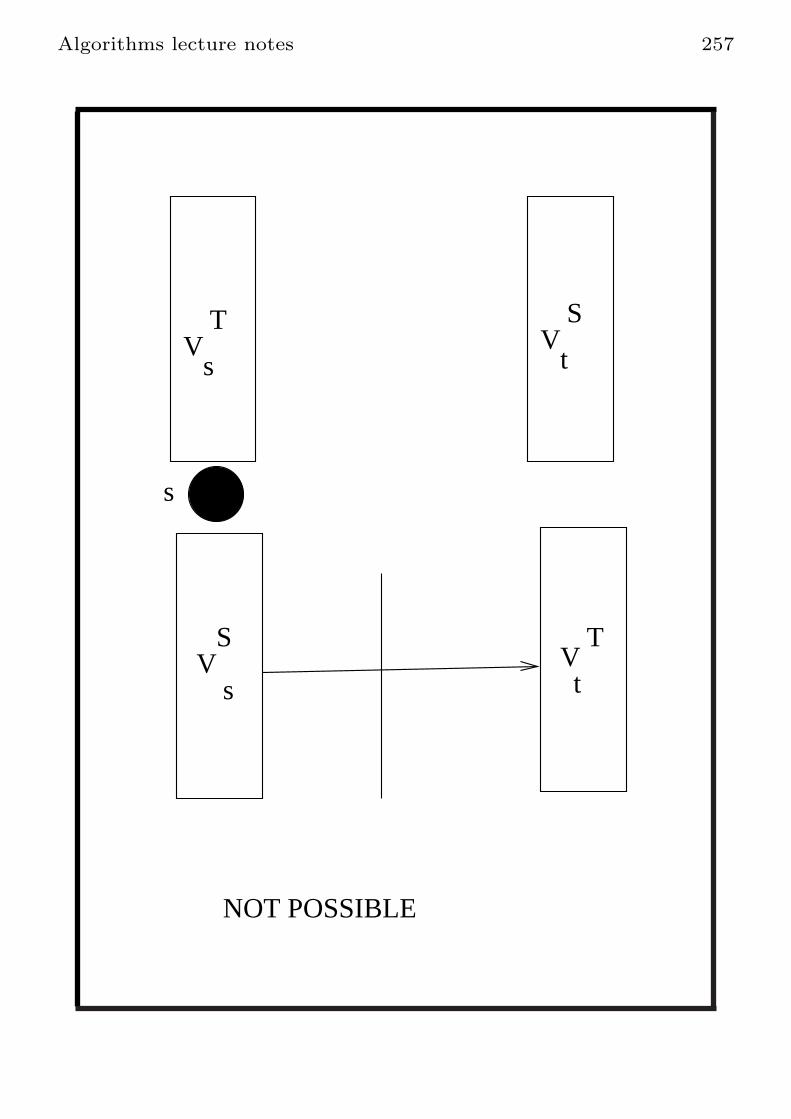
Algorithms lecture notes 257
VT
s
VS
s
s
VS
t
VT
t
NOT POSSIBLE

Algorithms lecture notes 258
A crucial property
The cut containing in the left side s and in
the right side V \ s has capacity of |V1|: thereare |V1| capacity 1 edge from s to all of V1.
Any edge from V S1 to V t
2 has capacity ∞.
Thus, it can not be the case that this edge will
participate in a minimum cut, as there are
finite cuts.
So there are no edges from any vertex in V S1 to
any vertex from V t2

Algorithms lecture notes 259
The size of the cut
We show that the capacity of the cut is
|V t1 |+ |V s
2 |.Check which edges go from the side of s in the
cut to the side of t. There are no edges from
V s1 to V t
2 by the previous answer.
The edges from V t1 to V s
2 are in the “wrong”
direction (from the side of t to the side of s and
not vice-versa).
There certainly are no edges from V s1 to V s
2 or
V s2 to V t
2 , because the graph is bipartite.
There are edges from s to V t1 , each edge of
capacity 1, so |V t1 | in total, and similarly, from
V s2 to t, with a capacity of V s
2 in total.
So, the minimum cut (or maximum flow)
equals |V t1 |+ |V s
2 |.

Algorithms lecture notes 260
V s
1∪ V t
2is a maximum independent
set
V s1 ∪ V t
2 is an independent set.
Under this restriction, we need to minimize
|V t1 |+ |V s
2 |, because this is the capacity of the
cut.
So, we maximize
(|V | − (|V t1 |+ |V s
2 |)) = |V s1 |+ |V t
2 |So V s
1 ∪ V t2 is a maximum independent set

Algorithms lecture notes 261
Finding undirected global min-cuts
The global minimum cut on an UNDIRECTED
graph is the partition S, .S, S, S 6= ∅ so that
e(S, S) = e = (u, v) : u ∈ S, v ∈ S isminimum.
If we know x ∈ S, y ∈ S, the following flow
network gives the cut:
1. Every edge e = (u, v) is replaced by two
edges u 7→ v and v 7→ u
2. Let x be source and y be sink
3. Compute the max flow, and min-cut
This takes O(n2) cut computation.
Improvement: fix x to be any vertex. Search
only for y (n flow computations)

Algorithms lecture notes 262
Finding global min-cuts
1. Every edge e = (u, v) is replaced by two
edges u 7→ v and v 7→ u
2. Let x be source and y be sink
3. Compute the max flow, and min-cut
This takes O(n2) cut computation.
Improvement: fix x to be any vertex. fearch
only for y (n flow computations)

Algorithms lecture notes 263
An amazingly simple algorithm
(Karger)
Works for graphs with parallel edges and
creates parallel edges.
1. Choose a pair of vertices to contract: If the
total numbe of edges be W and the number
of parallel edges between a and b be q, the
pair is chosen with probability q/W
/* A pair of vertices is more likely
to be chosen if it has many parallel edges
*/
2. Contract the pair of vertices chosen.
Retain parallel edges but delete self loops
3. Let G′ be the new graph
4. Recurse on G′

Algorithms lecture notes 264
Example
A
B
C
D
EF
B
AF E
C
D
B
AF EDC
ABF
ED
C
p=6/7
p=5/6
p=4/5
p=2/3
ABF CDE
P(MINIMUM)=6/7*5/6*4/5*2/3
Figure 1: The Karger algorithm

Algorithms lecture notes 265
The probability that the min-cut
results
Use:
Pr(A1 ∩A2 . . . ∩AK) = Pr(A1) · Pr(A2 | A1)
· Pr(A3 | A1 ∩A2) · . . .
Say that the min-size of the cut is k
So, deg(v) ≥ k for every v.
So |E| ≥ n · k/2Therefore, the probability that an edge in the
cut is not contracted is:
1− k
nk/2= 1− 2
n.

Algorithms lecture notes 266
Computation
(
1− 2
n
)
·(
1− 2
n− 1
)
·(
1− 2
n− 2
)
· . . .
·(
1− 2
4
)
·(
1− 2
3
)
·
=
(
n− 2
n
)
·(
n− 3
n− 1
)
·(
n− 4
n− 2
)
·
· 3
5· 24· 13
=2 · 1
n · (n− 1)

Algorithms lecture notes 267
A randomized alg with one sided
error probability
Run the algorithm n(n− 1)/2 times.
The probability that non of those runs give the
min-cut is at most:
(
1− 2
n(n− 1)
)n(n−1)/2
< 1/e
If we run it n2 · (n− 1)/2 times probability of
error at most exp(−n)