lecture notes for chapter 2 introduction to data...

© Tan,Steinbach, Kumar Introduction to Data Mining 4/18/2004 ‹#›

Data Mining: Data

Lecture Notes for Chapter 2

Introduction to Data Mining

by

Tan, Steinbach, Kumar


Similarity and Dissimilarity

� Similarity

– Numerical measure of how alike two data objects are.

– Is higher when objects are more alike.

– Often falls in the range [0,1]

� Dissimilarity

– Numerical measure of how different are two data objects

– Lower when objects are more alike

– Minimum dissimilarity is often 0

– Upper limit varies

� Proximity refers to a similarity or dissimilarity


Similarity/Dissimilarity for Simple Attributes

p and q are the attribute values for two data objects.


Euclidean Distance

� Euclidean Distance

Where n is the number of dimensions (attributes) and pk and qk

are, respectively, the kth attributes (components) or data objects p and q.

� Standardization is necessary, if scales differ.

∑=

−=n

kkk qpdist

1

2)(


Euclidean Distance

0

1

2

3

0 1 2 3 4 5 6

p1

p2

p3 p4

point x y

p1 0 2

p2 2 0

p3 3 1

p4 5 1

Distance Matrix

p1 p2 p3 p4

p1 0 2.828 3.162 5.099

p2 2.828 0 1.414 3.162

p3 3.162 1.414 0 2

p4 5.099 3.162 2 0


Minkowski Distance

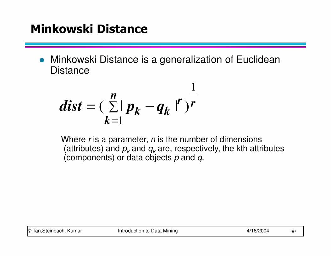
� Minkowski Distance is a generalization of Euclidean Distance

Where r is a parameter, n is the number of dimensions (attributes) and pk and qk are, respectively, the kth attributes (components) or data objects p and q.

rn

k

rkk qpdist

1

1

)||( ∑=

−=


Minkowski Distance: Examples

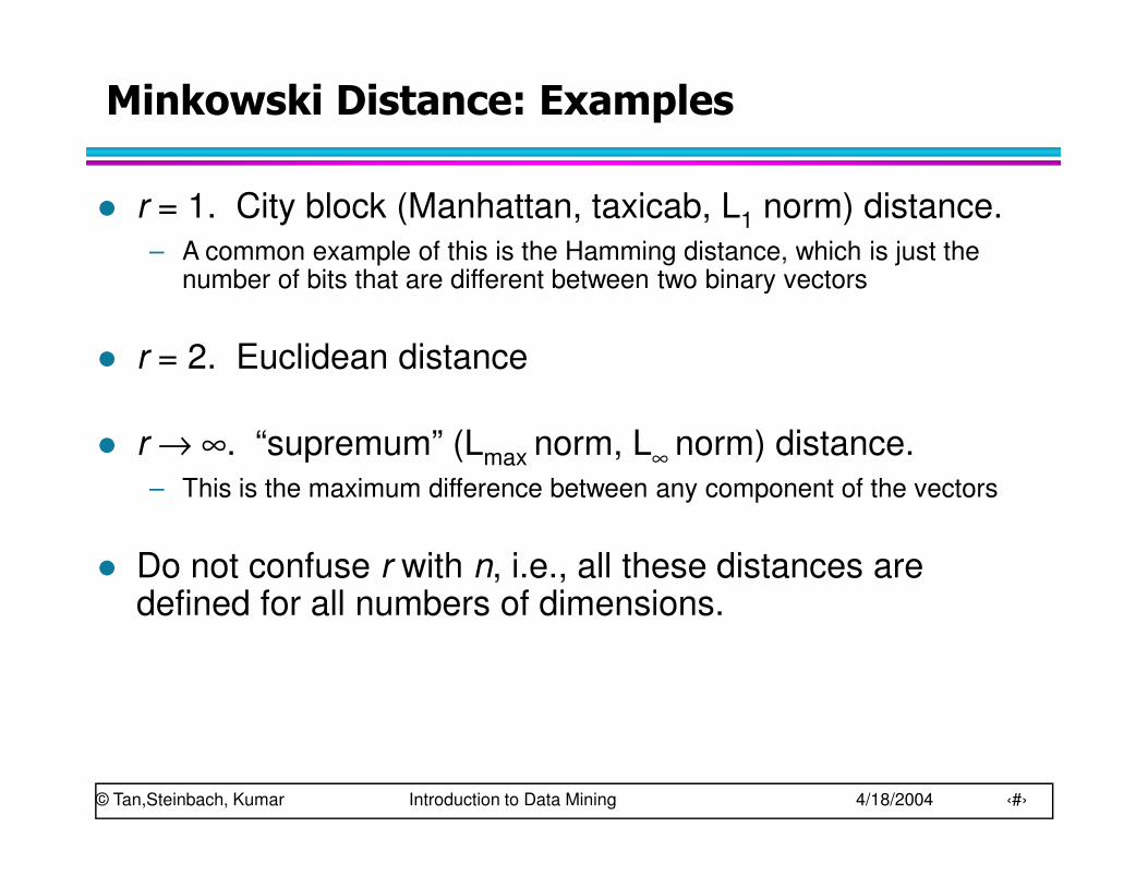
� r = 1. City block (Manhattan, taxicab, L1 norm) distance.

– A common example of this is the Hamming distance, which is just the number of bits that are different between two binary vectors

� r = 2. Euclidean distance

� r → ∞. “supremum” (Lmax norm, L∞

norm) distance.

– This is the maximum difference between any component of the vectors

� Do not confuse r with n, i.e., all these distances are defined for all numbers of dimensions.


Minkowski Distance

Distance Matrix

point x y

p1 0 2

p2 2 0

p3 3 1

p4 5 1

L1 p1 p2 p3 p4

p1 0 4 4 6

p2 4 0 2 4

p3 4 2 0 2

p4 6 4 2 0

L2 p1 p2 p3 p4

p1 0 2.828 3.162 5.099

p2 2.828 0 1.414 3.162

p3 3.162 1.414 0 2

p4 5.099 3.162 2 0

L∞∞∞∞ p1 p2 p3 p4

p1 0 2 3 5

p2 2 0 1 3

p3 3 1 0 2

p4 5 3 2 0


Mahalanobis Distance

Tqpqpqpsmahalanobi )()(),(1

−∑−=−

For red points, the Euclidean distance is 14.7, Mahalanobis distance is 6.

ΣΣΣΣ is the covariance matrix of the input data X

∑=

−−−

=Σ

n

i

kikjijkj XXXXn 1

, ))((1

1


Mahalanobis Distance

Covariance Matrix:

=Σ

3.02.0

2.03.0

B

A

C

A: (0.5, 0.5)

B: (0, 1)

C: (1.5, 1.5)

Mahal(A,B) = 5

Mahal(A,C) = 4


Common Properties of a Distance

� Distances, such as the Euclidean distance, have some well known properties.

1. d(p, q) ≥ 0 for all p and q and d(p, q) = 0 only if p = q. (Positive definiteness)

2. d(p, q) = d(q, p) for all p and q. (Symmetry)

3. d(p, r) ≤ d(p, q) + d(q, r) for all points p, q, and r. (Triangle Inequality)

where d(p, q) is the distance (dissimilarity) between points (data objects), p and q.

� A distance that satisfies these properties is a metric


Common Properties of a Similarity

� Similarities, also have some well known properties.

1. s(p, q) = 1 (or maximum similarity) only if p = q.

2. s(p, q) = s(q, p) for all p and q. (Symmetry)

where s(p, q) is the similarity between points (data objects), p and q.


Similarity Between Binary Vectors

� Common situation is that objects, p and q, have only binary attributes

� Compute similarities using the following quantitiesM01 = the number of attributes where p was 0 and q was 1

M10 = the number of attributes where p was 1 and q was 0



� Simple Matching and Jaccard Coefficients SMC = number of matches / number of attributes

= (M11 + M00) / (M01 + M10 + M11 + M00)

J = number of 11 matches / number of not-both-zero attributes values

= (M11) / (M01 + M10 + M11)


SMC versus Jaccard: Example

p = 1 0 0 0 0 0 0 0 0 0

q = 0 0 0 0 0 0 1 0 0 1

M01 = 2 (the number of attributes where p was 0 and q was 1)




SMC = (M11 + M00)/(M01 + M10 + M11 + M00) = (0+7) / (2+1+0+7) = 0.7

J = (M11) / (M01 + M10 + M11) = 0 / (2 + 1 + 0) = 0


Cosine Similarity

� If d1 and d2 are two document vectors, then

cos( d1, d2 ) = (d1 • d2) / ||d1|| ||d2|| ,

where • indicates vector dot product and || d || is the length of vector d.

� Example:

d1 = 3 2 0 5 0 0 0 2 0 0

d2 = 1 0 0 0 0 0 0 1 0 2

d1 • d2= 3*1 + 2*0 + 0*0 + 5*0 + 0*0 + 0*0 + 0*0 + 2*1 + 0*0 + 0*2 = 5

||d1|| = (3*3+2*2+0*0+5*5+0*0+0*0+0*0+2*2+0*0+0*0)0.5 = (42) 0.5 = 6.481

||d2|| = (1*1+0*0+0*0+0*0+0*0+0*0+0*0+1*1+0*0+2*2) 0.5 = (6) 0.5 = 2.245

cos( d1, d2 ) = .3150


Extended Jaccard Coefficient (Tanimoto)

� Variation of Jaccard for continuous or count

attributes

– Reduces to Jaccard for binary attributes


Correlation

� Correlation measures the linear relationship

between objects

� To compute correlation, we standardize data

objects, p and q, and then take their dot product

)(/))(( pstdpmeanpp kk −=′

)(/))(( qstdqmeanqq kk −=′

qpqpncorrelatio ′•′=),(


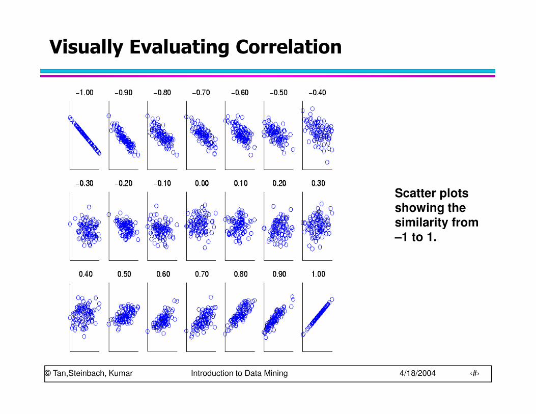
Visually Evaluating Correlation

Scatter plots

showing the similarity from

–1 to 1.


General Approach for Combining Similarities

� Sometimes attributes are of many different types, but an overall similarity is needed.


Using Weights to Combine Similarities

� May not want to treat all attributes the same.

– Use weights wk which are between 0 and 1 and sum to 1.


Density

� Density-based clustering require a notion of

density

� Examples:

– Euclidean density

� Euclidean density = number of points per unit volume

– Probability density

– Graph-based density


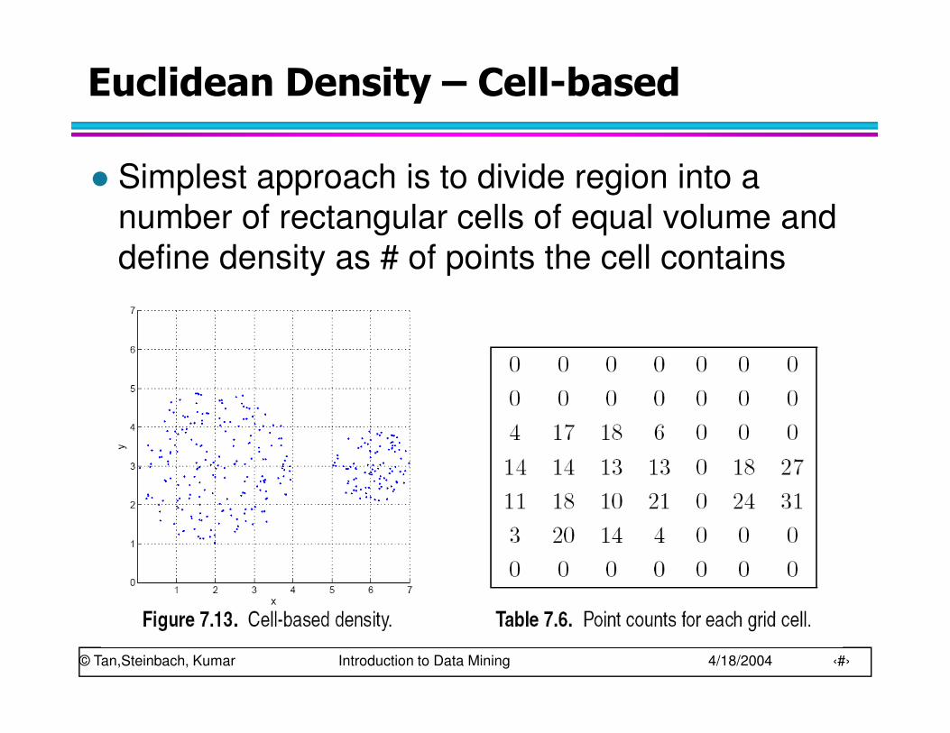
Euclidean Density – Cell-based

� Simplest approach is to divide region into a

number of rectangular cells of equal volume and

define density as # of points the cell contains


Euclidean Density – Center-based

� Euclidean density is the number of points within a

specified radius of the point

lecture notes for chapter 2 introduction to data...

Documents