Lecture Notes for Stat 375

Inference in Graphical Models

Andrea Montanari1

February 21, 2011

1Department of Electrical Engineering and Department of Statistics, Stanford University

Contents

1 Probability and graphs 21.1 Bayesian networks . . . . . . . . . . . . . . . . . . . . . . . . . . . . . . . . . . . . . . 21.2 Pairwise graphical models . . . . . . . . . . . . . . . . . . . . . . . . . . . . . . . . . . 41.3 Factor graphs . . . . . . . . . . . . . . . . . . . . . . . . . . . . . . . . . . . . . . . . . 4

1.3.1 Reduction from Bayesian networks to factor graphs . . . . . . . . . . . . . . . . 51.3.2 Reduction between to factor graphs . . . . . . . . . . . . . . . . . . . . . . . . 5

1.4 Markov random fields . . . . . . . . . . . . . . . . . . . . . . . . . . . . . . . . . . . . 61.5 Inference tasks . . . . . . . . . . . . . . . . . . . . . . . . . . . . . . . . . . . . . . . . 61.6 Continuous domains . . . . . . . . . . . . . . . . . . . . . . . . . . . . . . . . . . . . . 8

2 Inference via message passing algorithms 92.1 Preliminaries . . . . . . . . . . . . . . . . . . . . . . . . . . . . . . . . . . . . . . . . . 92.2 Trees . . . . . . . . . . . . . . . . . . . . . . . . . . . . . . . . . . . . . . . . . . . . . . 102.3 The sum-product algorithm . . . . . . . . . . . . . . . . . . . . . . . . . . . . . . . . . 122.4 The max-product algorithm . . . . . . . . . . . . . . . . . . . . . . . . . . . . . . . . . 122.5 Existence . . . . . . . . . . . . . . . . . . . . . . . . . . . . . . . . . . . . . . . . . . . 142.6 An example: Group testing . . . . . . . . . . . . . . . . . . . . . . . . . . . . . . . . . 152.7 Pairwise graphical models . . . . . . . . . . . . . . . . . . . . . . . . . . . . . . . . . . 162.8 Another example: Ising model . . . . . . . . . . . . . . . . . . . . . . . . . . . . . . . . 162.9 Monotonicity . . . . . . . . . . . . . . . . . . . . . . . . . . . . . . . . . . . . . . . . . 172.10 Hidden Markov Models . . . . . . . . . . . . . . . . . . . . . . . . . . . . . . . . . . . 18

3 Mixing 193.1 Monte Carlo Markov Chain method . . . . . . . . . . . . . . . . . . . . . . . . . . . . 19

3.1.1 Mixing time . . . . . . . . . . . . . . . . . . . . . . . . . . . . . . . . . . . . . . 203.1.2 Bounding mixing time using coupling . . . . . . . . . . . . . . . . . . . . . . . 213.1.3 Proof of the inequality (3.1.4) . . . . . . . . . . . . . . . . . . . . . . . . . . . . 223.1.4 What happens at larger λ? . . . . . . . . . . . . . . . . . . . . . . . . . . . . . 25

3.2 Computation tree and spatial mixing . . . . . . . . . . . . . . . . . . . . . . . . . . . . 253.2.1 Computation tree . . . . . . . . . . . . . . . . . . . . . . . . . . . . . . . . . . 25

3.3 Dobrushin uniqueness criterion . . . . . . . . . . . . . . . . . . . . . . . . . . . . . . . 30

4 Variational methods 324.1 Free Energy and Gibbs Free Energy . . . . . . . . . . . . . . . . . . . . . . . . . . . . 324.2 Naive mean field . . . . . . . . . . . . . . . . . . . . . . . . . . . . . . . . . . . . . . . 34

1

4.2.1 Pairwise graphical models and the Ising model . . . . . . . . . . . . . . . . . . 354.3 Bethe Free Energy . . . . . . . . . . . . . . . . . . . . . . . . . . . . . . . . . . . . . . 38

4.3.1 The case of tree factor graphs . . . . . . . . . . . . . . . . . . . . . . . . . . . . 394.3.2 General graphs and locally consistent marginals . . . . . . . . . . . . . . . . . . 414.3.3 Bethe free energy as a functional over messages . . . . . . . . . . . . . . . . . . 43

4.4 Region-Based Approximation of the Free Energy . . . . . . . . . . . . . . . . . . . . . 444.4.1 Regions and Region-Based Free Energy . . . . . . . . . . . . . . . . . . . . . . 444.4.2 Region-Based Approximation . . . . . . . . . . . . . . . . . . . . . . . . . . . . 464.4.3 Region Graph . . . . . . . . . . . . . . . . . . . . . . . . . . . . . . . . . . . . . 47

4.5 Generalized Belief Propagation . . . . . . . . . . . . . . . . . . . . . . . . . . . . . . . 484.6 Tree-based bounds . . . . . . . . . . . . . . . . . . . . . . . . . . . . . . . . . . . . . . 48

4.6.1 Exponential families . . . . . . . . . . . . . . . . . . . . . . . . . . . . . . . . . 494.6.2 Concavity of Bethe Free Energy on Trees . . . . . . . . . . . . . . . . . . . . . 51

4.7 Upper bound . . . . . . . . . . . . . . . . . . . . . . . . . . . . . . . . . . . . . . . . . 51

5 Learning graphical models 545.1 General setting and global approaches . . . . . . . . . . . . . . . . . . . . . . . . . . . 545.2 Local approaches: Parameter learning . . . . . . . . . . . . . . . . . . . . . . . . . . . 555.3 Local approaches: Structural learning . . . . . . . . . . . . . . . . . . . . . . . . . . . 58

2

Chapter 1

Probability and graphs

Graphical models are probability distributions that ‘factor’ according to a graph structure. Thespecific class of graph structures used and the precise meaning of ‘factor’ depend on the type ofgraphical model under consideration. Typically, factorization according to a graph encodes a specificclass of conditional independence properties.

There are two fundamental reasons that make graphical models interesting:

1. The class of probability distributions that factors accorting to a suitably sparse graph is alow-dimensional subclass of the set of all probability distribution over a given domain. Thisenables concise representation, and efficien learnability.

2. Sparse graph structures often correspond to weak dependencies, or to highly structured de-pendencies in the corresponding distributions. This leads to efficient algorithms for statisticalinference.

Specific families of graphical models include Bayesian networks, factor graphs, Markov randomfields. These allow to encode in various ways indepndency statements, and the choice of the mostsuitable formalism can be important in applications. On the other hand, they are loosely ‘reducible’to each other. By this we mean that a distribution that factors accordingly to a sparse graph structurein one formalism, also factors in other formalism according to a graph with the same sparsity.

This chapter provides a synthetic overview of the various formalisms. In the rest of the course, wewill focus on factor graphs but it is important to know how to pass from one formalism to another.

1.1 Bayesian networks

A Bayesian network describes the joint distributions of variables associated to the vertices of adirected acyclic graph G = (V,E), A directed graph is an ordinary graph with a direction (i.e. anordering of the adjacent vertices) chosen on each of its edges. The graph is acyclic if it has no directedcycle. In such a graph, we say that a vertex u ∈ V is a parent of v, and write u ∈ π(v), if (u, v)is a (directed) edge of G. A random variable Xv is associated with each vertex v of the graph (forsimplicity we assume all the variables to take values in the same finite set X ).

In a Bayesian network, the joint distribution of {Xv , v ∈ V } is completely specified by theconditional probability kernels {pv(xv|xπ(v))}v∈V , where π(v) denotes the set of parents of vertex v,and xπ(v) = {xu : u ∈ π(v)}. We also denote by π(G) the set of vertices that have no parent in G.

3

d1 d2 d3 d4 d5

f1 f2 f3 f4 f5 f6 f7 f8

Figure 1.1: Left: toy example of QMR-DT Bayesian network. Right: factor graph representation ofthe conditional distribution of the diseases d1, . . . d5, given the findings f1, . . . f8.

Given such a collection of conditional probabilities indexed by the vertices of G, we can constructin a unique way the joint distribution of all the variables µ on X V .

This is done according to the following definition.

Definition 1. Given a directed acyclic graph G = (V,E), and a probability distribution µ over X V ,we say that µ factors according to the Bayes network structure G (for short factors on G) if it canbe written as

µ(x) =∏

v∈π(G)

pv(xv)∏

v∈G\π(G)

pv(xv|xπ(v)) , (1.1.1)

for a set of conditional probability kernels p ≡ {pv}.If µ factors according to G, we say that the pair (G,µ) is a Bayesian network. Equivalently, we

will say that the triple (G, p,X ) is a Bayesian network.

Here is the conditional independence property encoded by G.

Proposition 1.1.1. The probability distribution µ over X V factors according to G if and only if,for each v ∈ V , and any S ⊆ V such that S∩descendants(v) = ∅, Xv is conditionally independent ofXS, given Xπ(v).

Here is an example showing the practical utility of Bayesian networks.Example: The Quick Medical Reference–Decision Theoretic (QMR-DT) network is a two level

Bayesian network developed for automatic medical diagnostic. A schematic example is shown inFig. 1.1. Variables in the top level, denoted by d1, . . . , dN , are associated with diseases. Variables inthe bottom level, denoted by f1, . . . , fM , are associated with symptoms or findings. Both diseases andfindings are described by binary variables. An edge connects the disease di to the finding fa wheneversuch a disease may be a cause for that finding. Such networks of implications are constructed on thebasis of accumulated medical experience.

The network is completed with two types of probability distributions. For each disease di we aregiven an a priori occurrence probability p(di). Furthermore, for each finding we have a conditionalprobability distribution for that finding given a certain disease pattern. This usually takes the socalled ‘noisy-OR’ form:

p(fa = 0|d) =1

zaexp

{−

N∑

i=1

θiadi

}. (1.1.2)

4

This network is to be used for diagnostic purposes. The findings are set to values determined by theobservation of a patient. Given this pattern of symptoms, one would like to compute the marginalprobability that any given disease is indeed present.

1.2 Pairwise graphical models

Pairwise graphical model are defined in terms of a simple graph G = (V, E) with vertex set V andedge set E . It is convenient to introduce a compatibility function ψi : X → R+ for each vertexi ∈ V, and one ψij : X × X → R+ for each edge (i, j) ∈ E . The joint distribution of (X1, . . . ,Xn),P(X = x) = µ(x) is then defined by

µ(x) =1

Z

∏

(i,j)∈E

ψij(xi, xj)∏

i∈V

ψi(xi) . (1.2.1)

The constant Z is called partition funtion and plays a quite important role. It is determined by thenormalization condition on µ, which implies

Z =∑

x∈XV

∏

(i,j)∈E

ψij(xi, xj)∏

i∈V

ψi(xi) . (1.2.2)

Example: A classical example of pairwise model is the Ising model from statistical physics. Inthis case X = {+1,−1}, and it is customary to parametrize the potentials in the form

ψij(xi, xj) = exp{Jijxixj

}, ψi(xi) = exp

{hixi

}. (1.2.3)

The same model is popular in machine learning under the name of Boltzmann machine (in thiscase one often takes xi ∈ {0, 1}. It includes as special cases some toy models for neural networks,such as the Hopfield model.

1.3 Factor graphs

A factor graph is a bipartite graph G = (V, F,E), whereby V and F are two (finite) sets of vertices,and E ⊆ V ×F a set of undirected edges. We will often identify V = [n] (set of the first n integers),F = [m]. We will call variable nodes the vertices in V , and use for them letters i, j, k, . . . , andfunction (or factor) nodes the vertices in F to be denoted by a, b, c . . . .

Given i ∈ V , the set of its neighbors is denoted by ∂i = {a ∈ F : (i, a) ∈ E}. The neighborhoodof a ∈ F , denoted by ∂a, is defined analogously.

A factor graph model (or graphical model) specifies the joint distribution of random variablesX = (X1, . . . ,Xn) = {Xi : i ∈ V } taking value in a domain X . As above, we shall assume1 that Xis a finite set. Indeed we shall mostly focus on the first case and write general equations in discretenotation. Finally, for any subset of variable nodes A ⊆ V , we write xA = {xi : i ∈ A}.

1In principle, the formalism can be defined whenever X is a measure space, but I do not know of any example thatis worth the effort.

5

Definition 2. The joint distribution µ over x ∈ X V factors on the factor graph G = (V, F,E) ifthere exists a vector of functions ψ = (ψ1, . . . , ψm) = {ψa : a ∈ F}, ψa : X ∂a → R+, and a constantZ such that

µ(x) =1

Z

∏

a∈F

ψa(x∂a) . (1.3.1)

We then say that the pair (G,µ) is a factor graph model. Equivalently, we will call the triple (G,ψ,X )a factor graph model.

The ψa’s are referred to as potentials or compatibility functions. The normalization constant isagain called the partition function and is given by

Z ≡∑

x

∏

a∈F

ψa(x∂a) . (1.3.2)

Notice that, in order for the distribution (1.3.1) to be well defined, there must be at least oneconfiguration x ∈ X V such that ψa(x∂a) > 0 for all a ∈ F . Checking this property is already highlynon-trivial, as shown by the following example.

Example. Let X = {0, 1}, G be a factor graph with regular degree k at factor notes, and forany a ∈ G let (x∗1(a), . . . , x

∗k(a)) ∈ X

∂a be given. Define

ψa(x∂a) = I(x∂a 6= x∗∂a) . (1.3.3)

The problem of checking whether this specifies a factor graph model is the k-satisfiability problemwhich is NP-complete. If it does, the resulting measure is the uniform measure over solutions of thek-satisfiability formula.

1.3.1 Reduction from Bayesian networks to factor graphs

Given a Bayesian network G and a set of observed variable O, it is easy to obtain a factor graphrepresentation of the conditional distribution p(xV \O|xO), by the following general rule is as follows:(i) associate a variable node with each non-observed variable (i.e. each variable in xV \O); (ii) foreach variable in π(G)\O, add a degree 1 function node connected uniquely to that variable; (iii) foreach non observed vertex v which is not in π(G), add a function node and connect it to v and to allthe parents of v; (iv) finally, for each observed variable u, add a function node and connect it to allthe parents of u.

1.3.2 Reduction between to factor graphs

Pairwise models can be reduced to factor graphs and viceversa.In order to get a reduction one has to construct, for any pairwise modelM, an associated factor

graph model M which describes the same distribution µ( · ), and viceversa. Reduction from pairwisemodels to factor graphs is straightforward. Use V as the set of variable nodes, and associate to eachedge (i, j) ∈ E and to each vertex V a factor node (in other words, set V = V and F ≃ V ∪ E).

Reduction from factor graphs to pairwise models is slightly less trivial. The basic idea is toreplace each factor node a by an ordinary vertex and associate to it a variable xa ∈ X

∂a which keepstrack of the values {xi :∈ ∂a}. We will fill the details in class.

6

1.4 Markov random fields

In order to reduce factor graph models to pairwise models, we had to enlarge the alphabet X . Ifyou do not like this, but still you prefer graphs to factor graphs, Markov random fields (sometimescalled Markov networks) are for you.

The underlying graph structure is an undirected graph G = (V,E).

Definition 3. The joint distribution µ over x ∈ X V is a Markov Random Field on G = (V, F,E)if there exists a vector of functions ψ = {ψC}C indexed by the cliques in G, ψC : XC → R+, and aconstant Z such that

µ(x) =1

Z

∏

C∈C

ψC(xC) . (1.4.1)

We then say that the pair (G,µ) (equivalently (G,ψ,X ))) is a Markov Random Field.

Reduction to and from factor graphs is trivial.The conditional independence property encoded in the graph structure is particularly crisp. Given

sets of vertices A,B,C ⊆ V , we say that C separates A from B if every path in G connecting avertex i ∈ A to a vertex j ∈ B has at least one vertex in C. We then have the following.

Theorem 1.4.1 (Hamersley, Clifford). If X = (Xi)i∈V is distributed according to a Markov RandomField (G,µ), then for any A,B,C ⊆ V , such that C separates A from B, XA is conditionallyindependent of XA, given XC .

Viceversa, if X ∼ µ, with µ(x) > 0 for all x ∈ X V is such that XA is conditionally independentof XA, given XC , for any A,B,C ⊆ V , such that C separates A from B, then µ is a Markov RandomField on G.

Proving the direct part is fairly obvious. The converse instead uses a clever construction of thefactors ψC( · ) form the probability distribution µ. At the moment do not need this construction, butwe will revisit Hammersley-Clifford theorem in Chapter 5.

1.5 Inference tasks

It is useful to keep in mind three inference problems that can be essentialy reduced to each other. Wedescribe them for factor graphs but little needs to be changed for other types of graphical models.

Computing marginals. Given a (typically small) subset of vertices A ⊆ V , compute theprobability P{XA = xA} = µ(xA).

Computing conditional probabilities. Given two subsets A, B ⊆ V , compute the condi-tional probability P{XA = xA|XB = xB} = µ(xA|xB).

Sampling. Sample a configuration of the random variables X ∼ µ.

Partition function. Compute the partition function Z, as per Eq. (eq:PartFun).

7

Reducibility between this tasks has been studied in detail in the Monte Carlo Markov Chain liter-ature within theoretical computer science: early references include [JVV86, JS89]. The ideas arestraightforward to describe informally.

Reduction between marginals and conditional probabilities. Obviously marginals are a special caseof conditional probabilities whereby B = ∅. In the opposite direction, computing the joint marginalµ(xA∪B) gives access to conditional probabilities via Bayes theorem.

A somewhat different way to obtain the second reduction consists in modifying the graphicalmodel. Namely, given an assignment x∗B to the variables in B construct the new model µ|B,x∗

Bby

adding for each node i ∈ B a new factor node with potebtial ψi(xi) = I(xi = x∗i ). It is then easy torealize that µ|B,x∗

B(xA) = µ(xA|x

∗B). Therefore computing conditional probabilities in the original

model is equivalent to computing marginals in the reduced model. We notice in passing that sincethe variables in B are fixed once and for all, we might as well eliminate them in the obvious way.We obtain a new model with vertex set V \B and factors ψa|B,x∗

B.

Reduction from marginals to sampling. If we can sample one configuration, we can as well samplemany of them X(1),X(2), . . . ,X(M). Estimate tha marginals of µ(xA) with the empirical distributionof xA in this sample. As long as A is bounded, precision ε can be achieved with probability latgerthan (1− δ) with O(ε−1/2 log(1/δ)) samples.

Reduction from sampling to marginals. Order the variable nodes arbitrarily, say 1, 2, 3, . . .n.Compute the marginal of the first variable µ(x1) and sample from it (this is easy because the alphabet

X is small). Let x∗1 be this sample. Reduce the model, by letting V1 = V \ {1} and ψ(1)a = ψa|{1},x∗

1.

Repeat.

Reduction from marginals to partition function. Let Z|A,x∗A

be the partition function of thereduced model. Then we have the identity

µ(x∗A) =Z|A,x∗

A

Z, (1.5.1)

which immediately yields the desired reduction.

Reduction from marginals to partition function. Again order variables as 1, 2, 3, . . .n, and choosespecial values x∗1, x

∗2, x

∗3, . . . x∗n. Also let A(ℓ) = {1, 2, . . . , ℓ} ⊆ V . We then have

Z =Z

Z|A(1),x∗A(1)

Z|A(1),x∗A(1)

Z|A(2),x∗A(2)

. . .Z|A(n−1),x∗

A(n−1)

Z|A(n),x∗A(n)

Z|A(n),x∗A(n)

. (1.5.2)

The last term is trivial to compute since

Z|A(n),x∗A(n)

=∏

a∈F

ψa(xa) . (1.5.3)

As for the n ratios they are just marginals. Indeed the identity (1.5.1) yields

Z|A(ℓ+1),x∗A(ℓ+1)

Z|A(ℓ),x∗A(ℓ)

= µ|A(ℓ),x∗A(ℓ)

(x∗ℓ+1) , (1.5.4)

which implies the claimed reduction.

8

1.6 Continuous domains

In the case X = R, Eq. (1.3.1) defines the density of (X1, . . . ,Xn) with respect to the productLebesgue measure (the ψa’s have to be measurable in this case).

9

Chapter 2

Inference via message passingalgorithms

Belief propagation (BP) is an umbrella term describing a family algorithms for approximate inferencein graphical models. These algorithms are also collectively referred to as message passing algorithms.Both of these are somewhat loose terms, but generally convey the idea that algorithms in this classproceed by updating estimates of local marginals of the graphical model µ. Local marginals areupdated by using information about marginals at neighboring nodes that is ‘passed’ along edges inthe graph.

2.1 Preliminaries

Throughout this chapter we will consider the factor graph model

µ(x) =1

Z

∏

a∈F

ψa(xa) , (2.1.1)

defined on the factor graph G = (V, F,E), and alphabet X ∋ xi.Consistently with our discussion of reduction between various inference tasks, we will focus on

the problem of computing local marginals, i.e. marginal distributions of a small subset of variables,e.g. µA(xA) = Pµ{XA = xA}. Explicitely

µA(xA) =∑

xV \A

µ(x) . (2.1.2)

To be definite, you can think of simple ‘one-point’ marginals A = {i}. The most popular message-passing algorithm for computing marginals is known as the sum-product algorithm.

One can define a natural analogous of marginals when the problem is the one of computing themode of µ. These are called, for lack of better ideas, ‘max marginals’. For A ⊆ V , the max marginalis deined as

MA(xA) = maxxV \A

µ(x) . (2.1.3)

10

2

3

4

b

a

c

5

6

0

1

Figure 2.1: A small tree.

What is a max-marginal good for? Say that you computed MA(xA). Then it is easy to see that,for any x∗A ∈ arg maxxA

MA(xA), there exists an extension of x∗A to a mode if µ. The analogous ofthe sum-product algorithm for computing max-marginals is known as the max-product algorithm (orsometimes min-sum algorithm).

In the following we will often have to write identites in which the overall normalization of bothsides is not really interesting. In order to get rid of all these normalization floating around, it isconveniet to use a special notation. Throughout this course, the symbol ∼= is used to denote equalitybetween functions up to a multiplicative normalization. Formally, we shall write f(x) ∼= g(x) if thereexist a non-vanishing constant A such that f(x) = Ag(x) for all x.

Sometimes the symbol ∝ is used for the same purpose. Since ∝ has actually is somewhat morevague, I will avoid this symbol.

2.2 Trees

Inference is easy if the underlying factor graph is a tree. By ‘easy’ we mean that it can be performed intime linear in the number of nodes, provided the factor nodes have bounded degree and the alphabetsize is bounded as well. The algorthm that achieves this goal is a symple ‘dynamic programming’procedure.

Let us see how this works on the simple example reproduced in Fig. ??. We begin by assumingthat we want to compute the marginal at node 0:

µ(x0) ∼=∑

xV \0

∏

ℓ∈F

ψℓ(xℓ) . (2.2.1)

Node 0 is the root of three subtrees of G, that we can distinguish by the name of the factor nodeneighbor of 0 that they contain, namely Ga→0 = (Va→0, Fa→0, Ea→0), Gb→0 = (Vb→0, Fb→0, Eb→0),

11

Gc→0 = (Vc→0, Fc→0, Ec→0). We can rewrite the sum in Eq. (2.2.1) as (for such a small graph it is abit of an overkill but bear with me)

µ(x0) ∼=∑

xV \0

∏

ℓ∈Fa→0

ψℓ(xℓ)∏

ℓ∈Fb→0

ψℓ(xℓ)∏

ℓ∈Fc→0

ψℓ(xℓ)

∼={ ∑

xVa→0\0

∏

ℓ∈Fa→0

ψℓ(xℓ)}·{ ∑

xVb→0\0

∏

ℓ∈Fb→0

ψℓ(xℓ)}{ ∑

xVc→0\0

∏

ℓ∈Fc→0

ψℓ(xℓ)}

∼= µa→0(x0)µb→0(x0)µc→0(x0) .

Here in the second line we used the distributive property to ‘push’ the sums through the product offactor terms. In the last step we defined µa→0(x0) that is the marginal with respect to the factorgraph Ga→0.

Thus we reduced the problem of computing a marginal with respect to G to the ones of computingmarginals with respect to subgraphs of G. We can repeat this recursively. Consider the subtree Ga→0.This can be decomposed into the factor node a, plus the subtrees G1→a and G2→a. Using again thedistributive property we have

µa→0(x0) ∼=∑

xVa→0\0

∏

ℓ∈Fa→0

ψℓ(xℓ)

∼=∑

x1,x2

ψa(xa){ ∑

xV1→a\1

∏

ℓ∈F1→a

ψℓ(xℓ)}{ ∑

xV2→a\2

∏

ℓ∈F2→a

ψℓ(xℓ)}

∼=∑

x1,x2

ψa(xa)µ1→a(x1)µ2→a(x2) .

It is quite clear that our arguments did not use the specific structure of the factor graph inFig. 2.1. But they instead hold for any tree. Namely given a tree G and a directed edge a → i(factor-to-variable) or i→ a (variable-to-factor) we can define the subgraphs Ga→i or Gi→a as aboveand the corresponding ‘partial marginals’ of the variable i: µa→i(xi) and µi→a(xi). We will also callthese messages. We then have the following

Proposition 2.2.1. For a tree graphical model, the ‘partial marginals’ are the unique solution of theequations

µj→a(xj) ∼=∏

b∈∂j\a

µb→j(xj) , (2.2.2)

µa→j(xj) ∼=∑

x∂a\j

ψa(x∂a)∏

k∈∂a\j

µk→a(xk) , (2.2.3)

For all (i, a) ∈ E.

Notice that both existence and uniqueness follow from the recursive argument discussed above.It should also be clear that marginals of µ can be computed easily in terms of partial marginals. Wehave for instance:

µi(xi) ∼=∏

a∈∂i

µa→i(xi) , (2.2.4)

µa(xa)∼= ψa(xa)

∏

i∈∂a

µi→a(xi) . (2.2.5)

12

2.3 The sum-product algorithm

The sum product algorithm is an iterative message passing algorithm. The basic variables are‘messages’ which are probability distributions over X . These are also called ‘beliefs’. Two suchdistributions are used for each edge in the graph νi→a( · ) (variable to factor node) νa→i( · ) (factorto variable node). We shall denote the vector of messages by ν = {νi→a, νa→i}: it is a vector ofprobability distributions, indexed by directed edges in G.

We shall indicate the iteration number by supercripts, e.g. ν(t)i→a, ν

(t)a→i are the messages value

after t iterations. Messages are initialized to some non-informative values, typically ν(0)i→a, ν

(0)a→i are

equal to the uniform distribution over X .Various update scheduling are possible, but for the sake of simplicity we will consider parallel

updates, which read:

ν(t+1)j→a (xj) ∼=

∏

b∈∂j\a

ν(t)b→j(xj) , (2.3.1)

ν(t)a→j(xj) ∼=

∑

x∂a\j

ψa(x∂a)∏

k∈∂a\j

ν(t)k→a(xk) . (2.3.2)

It is understood that, when ∂j \ a is an empty set, νj→a(xj) is the uniform distribution.After t iterations, one can estimate the marginal distribution µ(xi) of variable i using the set of

all incoming messages. The BP estimate is:

ν(t)i (xi) ∼=

∏

a∈∂i

ν(t−1)a→i (xi) . (2.3.3)

The rationale for Eqs. (2.3.1) and (2.3.2) is easy to understand given the discussion in the previoussection: we are trying to iteratively find solutions of Eqs. (2.2.2), (2.2.3). These exactly hold forpartial marginals on trees. On general graphs, the resulting fixed points will not be necessarilymarginals of µ, but te hope is that they are nevertheless a good approximation of the actual marginals.We use a different letter (ν instead of µ) to emphasize the fact that messages do not coincide in generalwith marginals.

We formalize the connection between the sum-product algorithm and tree graphical model asfollows.

Proposition 2.3.1. If G is a tree, then the sum-product algorithm converges in diam(G) iterationto its unique fixed point νi→a = µi→a, νa→i = µa→i. The resulting estimates for the marginals, cf.Eq. (2.3.3) are exact.

2.4 The max-product algorithm

Max-product updates are used to approximately find the mode of a distribution specified by a factorgraph model. Before discussing the algorithm, it is useful to show how mode computation can beeffectively reduced to the computation of max-marginals. Recall that the mode of µ, cf. Eq. (2.1.1)is any assignment x∗ ∈ X V of maximal probability, i.e.

x∗ ∈ arg maxx∈XV

∏

a∈F

ψa(xa) . (2.4.1)

13

Order the variables arbitrarily, say 1, 2, . . . , n. Compute the max-marginal of x1, call it M1(x1) and

choose x∗1 ∈ arg maxx1∈X M1(x1). Reduce the model by , by letting V1 = V \{1} and ψ(1)a = ψa|{1},x∗

1.

Compute the max-marginal of variable 2 in the reduced model M(1)2 (x2) and repeat.

Vice-versa, computing max-marginals is easy if we have at our disposal a routine to compute themode of a graphical model. Suppose that the variable of interest is xi. We have

Mi(xi) ∼= maxxV \{i}

∏

a∈F

ψa|{i},xi(xa) , (2.4.2)

which is requires obtained from the computation of the mode of the reduced graphical model.The derivation of the max-product algorithm closely parallels the one of the sum-prosuct algo-

rithm. (Indeed the two can be put in a unified framework using the so-called ‘generalized distributiveproperty’ [AM00].) Again consider first the case of a tree graphical model. One can define subtreesGi→a, Ga→i analogously to what we did for the sum-product algorithm, and the correspondingmessages as

Mi→a(xi) ∼= maxxVi→a\i

∏

b∈Fi→a

ψb(xb) , (2.4.3)

Mi→a(xi) ∼= maxxVa→i\i

∏

b∈Fa→i

ψb(xb) . (2.4.4)

Proceeding as for the sum-product algorithm, it is then easy to show that these marginals are theunique solution of the equations

Mj→a(xj) ∼=∏

b∈∂j\a

Mb→j(xj) , (2.4.5)

Ma→j(xj) ∼= maxx∂a\j

{ψa(x∂a)

∏

k∈∂a\j

Mk→a(xk)}, (2.4.6)

with one equation per edge in G.The above equations for a tree motivate the following iterative algorithm

ν(t+1)i→a (xi) ∼=

∏

b∈∂i\a

ν(t)b→i(xi) , (2.4.7)

ν(t)a→i(xi) ∼= max

x∂a\i

ψa(x∂a)

∏

j∈∂a\i

ν(t)j→a(xj)

. (2.4.8)

The max-marginals are then estimated as

ν(t)i (x∗i )

∼=∏

b∈∂i\a

ν(t)b→i(xi) , . (2.4.9)

The name of the max-product algorithm has obvious origins. Sometimes, the same algorithmis also called min-sum because is written in a slightly different form. Instead of maximizing the

14

probability, one starts from the equivalent problem of minimizing a cost function that factorizesaccording to G:

H(x) =∑

a∈F

Ha(x∂a) . (2.4.10)

The min-sum update equations read

J(t+1)i→a (xi) = const. +

∑

b∈∂i\a

J(t)b→i(xi) , (2.4.11)

J(t)a→i(xi) ∼= min

x∂a\i

Ha(x∂a) +

∑

j∈∂a\i

J(t)j→a(xj)

. (2.4.12)

They can be obtained from the max-product updates via the identification ν(t)i→a(xi) ∼= exp{−J

(t)i→a(xi)}

and ν(t)a→i(xi) ∼= exp{−J

(t)a→i(xi)}

An analogous of Proposition 2.3.1 holds for the max-product algorithm: On tree graphical modelsthe max-product algorithm converges to the correct max-marginals after diam(G) iterations.

2.5 Existence

Let ~E denote the set of directed edges (whereby each edge (i, a) corresponds to two directed edgesi→ a and a→ i), and M(X ) the set of probability distributions over X (i.e. the (|X |−1)-dimensional

simplex). Then the space of messages is M(X )~E ∋ ν. The sum-product BP update defines a non-

linear mapping

TG : M(X )~E → M(X )

~E ,

ν 7→ TG(ν) .

For the sake of completeness, let me copy here the definition of such a mapping. If ν′ = TG(ν), then

ν ′j→a(xj) ∼=∏

b∈∂j\a

νb→j(xj) , (2.5.1)

ν ′a→j(xj) ∼=∑

x∂a\j

ψa(x∂a)∏

k∈∂a\j

νk→a(xk) . (2.5.2)

Notice that a distribution µ(x) admits (in general) more than one decomposition of the form (??).On the other hand:

Remark 1. The mapping TG depends on the factor graph G and on the potentials ψ.

If G is a tree (or a forest), TG admits a unique fixed point. What happens on general graphs G?A large number of cases is covered by the following definition.

Definition 4. We say that the pair (G,ψ) is permissive if, for each i ∈ V , there exists x∗i ∈ X suchthat

ψa(x∗i , x∂a\i) ≥ ψmin > 0 , (2.5.3)

for each x∂a\i ∈ X∂a\i and a ∈ ∂i.

15

Then we have the following simple result.

Proposition 2.5.1. If the factor graph model (G,ψ) is permissive, then the BP operator TG admitsat least one fixed point.

Proof. We will only sketch the main ideas, leaving details to the reader. The proof indeed a directapplication of the following well known result in topology.

Theorem 2.5.2 (Brouwer’s fixed point theorem). Let f : BN → BN be a continuous mapping fromthe N -dimensional closed unit ball BN = {z ∈ R : ||z|| ≤ 1} to itself. Then f admits at least onefixed point.

Since this is a theorem about continuous functions, it generalizes to any domain D that is home-omorphic to BN . (Indeed, if ϕ : BN → D is such an homeomorphism, and g : D → D is the mappingof interest, set f = ϕ−1 ◦ g ◦ ϕ.)

The theorem is then applied to TG : M(X )~E → M(X )

~E . To finish the proof, one has to check

that: (i) M(X )~E is homeomorphic to a unit ball; (ii) TG is continuous. In the second step, one uses

the permissivity assumption.

2.6 An example: Group testing

Let us reconsider the group testing example. Recall that the we want to make inference on variablesx = (x1, . . . , xn), xi ∈ {0, 1} (causes), given observations y = (y1, . . . , ym), ya = ∨i∈∂axi (symptoms).We assume that, a priori, the xi’s are iid Bernoulli(p). As usual, we consider the factor graphG = (V, F,E) where V = [n], F = [m], and (i, a) ∈ E if and only if i ∈ V is among the causes ofa ∈ F . We further let F = F0 ∪ F1, where F0/1 ≡ {a ∈ F : ya = 0/1}.

µ(x) =1

Z

∏

a∈F0

I(x∂a = 0)∏

a∈F1

I(x∂a 6= 0)∏

i∈V

pxi(1− p)1−xi . (2.6.1)

We could write down the BP update rules for this model (and the reader is indeed invited to doso) but it is more convenient to simplify it a bit. If ya = 0, then we know that xi = 0 for each i ∈ ∂a.We can thus reduce the factor graph by eliminating all f-nodes in F0, and all adjacent v-nodes. Nextif a ∈ F1 has only one adjacent node i ∈ V , then we know that xi = 1. We can than recursivelyeliminate all such nodes. At the end of such process we are left with a subgraph G′ = (V ′, F ′, E′)with V ′ ⊆ V , F ′ ⊆ F1, and each node a ∈ F ′ having degree |∂a| ≥ 2. The joint distribution

µ(x) =1

Z

∏

a∈F ′

I(x∂a 6= 0)∏

i∈V ′

pxi(1− p)1−xi . (2.6.2)

Is this graphical model permissive?Messages are distributions over binary variables. Each term pxi(1 − p)1−xi can be described

by a factor node of degree one. The corresponding message directed towards i is fixed to ν, withν(0) = 1 − p, ν(1) = p. Since this message does not change over time, we will only write the BP

16

update equations for other edges. They read

ν(t+1)i→a (xi) ∼= ν(xi)

∏

b∈∂i\a

ν(t)b→i(xi) , (2.6.3)

ν(t)a→i(xi) ∼=

{1−

∏j∈∂a\i ν

(t)j→a(0) if xi = 0,

1 if xi = 1.(2.6.4)

Distributions over binary variables can be parametrized by a single real number. For instance, wecan use the probability of 0. If we let vi→a ≡ νi→a(0) and va→i ≡ νa→i(0), we obtain the equations

v(t+1)i→a =

(1− p)∏

b∈∂i\a v(t)b→i

(1− p)∏

b∈∂i\a v(t)b→i + p

∏b∈∂i\a(1− v

(t)b→i)

, (2.6.5)

v(t)a→i = 1−

1

2−∏

j∈∂a\i v(t)j→a

. (2.6.6)

Using these messages, one can estimate the a posteriori probability that cause i is present as

ν(t+1)i (xi = 1) =

p∏

b∈∂i(1− v(t)b→i)

(1− p)∏

b∈∂i v(t)b→i + p

∏b∈∂i(1− v

(t)b→i)

. (2.6.7)

2.7 Pairwise graphical models

Since pairwise graphical models are reducible to factor fraph (and indeed are a special type of factorgraph whereby all factors have degree 2) we could in principle skip this section altogether. On theother hand, they are an important subclass, and it is instructive to write equations explicitely in thiscase.

We consider the model

µ(x) =1

Z

∏

(i,j)∈E

ψij(xi, xj)∏

i∈V

ψi(xi) . (2.7.1)

Adapting Eqs. (2.3.1), (2.3.2) is straightforward. We can associate one factor node a to each edge(i, j) and hence will have messages νi→(i,j) and ν(i,j)→j. However, the latter is a simple function ofthe former:

ν(t)(i,j)→j(xj) ∼=

∑

xi

ψij(xi, xj)ν(t)i→(i,j)(xi) . (2.7.2)

We thus can eliminate ν(t)(i,j)→j completely, and write simple updates for ν

(t)i→(i,j), that we will denote

as ν(t)i→j. Notice that in principle we should also introduce a factor node a for each singleton term

ψi(xi), but the corresponding message would be νa→i(xi) ∼= ψi(xi) and we can eliminate it as well.We finally obtain the update rules

ν(t+1)i→j (xi) ∼= ψi(xi)

∏

k∈∂i\j

{∑

xk

ψik(xi, xk)νk→i(xk)}. (2.7.3)

17

2.8 Another example: Ising model

Recall that the Ising model is a pairwise model on the graph G = (V,E) whose distribution takesthe form

µ(x) =1

Zexp

{ ∑

(i,j)∈E

Jijxixj +∑

i∈V

hixi

}, (2.8.1)

with xi ∈ X ≡ {+1,−1} (any pairwise nmodel on binary variables can be written in this form).It is immesiate to adapt the sum-product update (2.7.3) to the present case. We get

ν(t+1)i→j (xi) ∼= ehixi

∏

k∈∂i\j

{ ∑

xk∈{+1,−1}

eJikxixkνk→i(xk)}. (2.8.2)

Since xi takes two values, it is sufficient to specify one real parameter for message. It is customaryin many applications to use log-likelihood ratios, i.e.

h(t)i→j ≡

1

2log{ν(t)

i→j(+1)

ν(t)i→j(−1)

}. (2.8.3)

In terms of these variables, the update becomes (after a tedious calculus exercise)

h(t+1)i→j = hi +

∑

k∈∂i\j

atanh{

tanh(Jik) tanh(h(t)k→i)

}. (2.8.4)

Where tanh and atanh are hyerbolic tangent and arctangent.

2.9 Monotonicity

Consider again the group testing example. Notice that, according to Eq. (2.6.5), the output of afunction node is monotonically decreasing in its inputs. On the other hand, by Eq. (2.6.6), theoutput of a function node is monotonically increasing in its inputs. It follows that the BP iterationis anti-monotone in the following sense.

Consider the vector of variable-to-function node messages, and denote it, with an abuse of nota-tion, by ν = {νi→a( · ) : (i, a) ∈ E}. Let T∗

G be the mapping degined by one full BP iteration appliedto this set of messages. We write ν � ν ′ if, for each (i, a) ∈ E, νi→a(1) ≤ ν ′i→a(1). This is a partialordering on the space of message sets.

The above remarks imply that, if ν � ν ′, then T∗G(ν) � T∗

G(ν ′). This remarks has some interesting

consequences. Imagine to initialize messages in such a way that ν(0)i→a(0) = 1 for each directed edge

i → a. Then ν(1) � ν(0) necessarily. By applying (T∗G)t to this inequality, we get that ν(t+1) � ν(t)

for t even, and ν(t+1) � ν(t) for t odd: messages ‘toggle’. By the same token ν(2) � ν(0). Applyting(T∗

G)t, we get that the sequence of messages at even times is monotone increasing, and the one atodd times is monotone decreasing. In particular The two sequences converge to a pair of fixed pointsof (T∗

G)2.

Another example of the utility of monotonicity arguments is provided by the Ising model, dis-cussed in section 2.8. If the interaction parameters are all non-negative, Jij ≥ 0, then this updateis monotone increasing. It is then easy to show that BP always converges if initialized, for instance,

with h(0)i→j = 0.

18

2.10 Hidden Markov Models

A (homogeneous) Markov Chain over the state space X is a sequence of random variables X =(X0,X1, . . . ,Xn) whose joint distribution takes the form

P{X = x} = p0(x0)

n−1∏

i=0

p(xi+1|xi) , (2.10.1)

for some initial distribution p0 and conditional probability kernel p(xi+1|xi).An Hidden Markov Model arises when partial/noisy observations of the chain are available. The

joint distribution of the chain X and of the observations Y reads

P{X = x, Y = y} = p0(x0)

n−1∏

i=0

p(xi+1|xi)

n∏

i=0

q(yi|xi) , (2.10.2)

where q describes the observation process.A common computational task is the one of inferring the sequence of states x from the observa-

tions. For this task, it makes sense to consider the conditional probability distribution of X giventhe observations, which by Bayes theorem takes the form

P{X = x|Y = y} ∼= p0(x0)n−1∏

i=0

p(xi+1|xi)n∏

i=0

q(yi|xi) . (2.10.3)

This is easily represented as a pairwise graphical model whose underlying graph is a chain. We getindeed (assuming y fixed once and for all) P{X = x|Y = y} = µ(x), where

µ(x) =1

Z

n−1∏

i=0

ψi(xi, xi+1) , (2.10.4)

ψ0(x0, x1) = p0(x0)p(x1|x0) q(y0|x0) , (2.10.5)

ψi(xi, xi+1) = p(xi+1|xi) q(yi|xi) i ≥ 1 . (2.10.6)

The sum-product update is straightforwarly written for this case

νi→i+1(xi) ∼=∑

xi−1

ψi−1(xi−1, xi)νi−1→i(xi−1) , (2.10.7)

νi→i−1(xi) ∼=∑

xi+1

ψi(xi, xi+1)νi+1→i+(xi) . (2.10.8)

Notice that since the graph is a tree, the algorithm is guaranteed to converge, and it is sufficient asingle pass forward and a single pass backwards. Indeed the algorithm has been well-known for along time as the forward-backward algorithm.

19

Chapter 3

Mixing

We will begin by introducing the Monte Carlo Markov Chain method. This is a randomized algorithmthat can be use to compute marginals of a graphical model. We will see that MCMC is guaranteedto work when distinct variables in the graphical model are not too strongly correlated. We will thenintroduce the computation tree: a very useful construction for analyzing message passing algorithms.In particular, the behavior of such algorithms is related to the strenght of correlations on such trees.

3.1 Monte Carlo Markov Chain method

Given a model defined on the factor graph G = (V = [n], F,E):

µ(x) =1

Z

∏

a∈F

ψa(x∂a) , (3.1.1)

where x ∈ X V , the Monte Carlo method tries to estimate its marginal by sampling x(1), . . .x(N)

approximately iid from µ( · ). In order to obtain iid samples, we introduce an irreducible and aperiodicMarkov Chain that has µ as its stationary measure.

To be concrete, we will focus on a siggle example throughout this lecture (but wath we shall saycan indeed be generalized). Given G = (V, E), sample independent sets with probability

µ(x) =1

Z

∏

(i,j)∈E

I((xi, xj) 6= (1, 1)

)∏

i∈V

λxi (3.1.2)

where xi ∈ X = {0, 1}.Metropolis dynamics allows to define a Markov chain with µ as its stationary measure. The

chain is identified by the matrix of transition probabilities {p(x, y)}x,y∈XV , whereby p(x, y) is theprobability that the configuration at time t + 1 is y, given that at time t it is x. In the case ofMetropolis dynamics, they satisfy the so-called reversibility condition

µ(x)p(x, x′) = µ(x′)p(x′, x) . (3.1.3)

This in particular implies that µ is a stationary measure for the chain.For our example, Metropolis dynamics can be described as follows:

20

• Given the current configuration x, first choose i ∈ V uniformly at random.

• Set x′j = xj∀j 6= i, and choose x′i ∈ {0, 1} uniformly at random. This is the “proposed” move.

• The proposal is accepted with probability

π = min {1, λxi−xi}

if all the neighbors of i are empty. Otherwise, π = 0.

The transition rule can also be specified as follows.If xi = 1,

x′i =

{0 with prob 1

2min(1, λ−1)xi otherwise

If xi = 0,

x′i =

{1 if xj = 0 ∀j ∼ i and with prob 1

2min(1, λ)xi otherwise

Notice that with probability half, x does not change. It is also immediate to see that the chainis irreducible: for any two independent sets x, y, there exists a sequence of transitions with nonvanishing probability that bring from x to y. You are invited to check that the chain is indeedreversible with respect to µ( · ). This implies that µ( · ) is indeed the unique stationary measure.

3.1.1 Mixing time

After defining a Markov chain with µ as its stationary measure, we start from an arbitrary config-uration x(0), eg. an empty independent set, and run the transitions for t steps. We “pretend” thatthe configuration x(t) is distributed according to µ( · ) to compute the desired marginal. If we denoteby µ(t) the distribution of x(t), we would like

µ(t)(x) ≈ µ(x)

In order to make this idea more precise, we define

Total variation distance

‖µ(t) − µ‖TV ≡1

2

∑

x

|µ(t)(x)− µ(x)|

and

Mixing timeτmix(ǫ) = sup

x0

inf{ τ : ‖µ(t) − µ‖TV ≤ ǫ∀t ≥ τ}

Notice that

‖µ(t) − µ‖TV ≤ ǫ⇒ |∑

x

f(x)µ(t)(x)−∑

x

f(x)µ(x)| ≤ 2ǫ supx|f(x)|

In particular, singular variable marginals are well aproximated

|µ(t)i (xi)− µ(xi)| ≤ ǫ

21

3.1.2 Bounding mixing time using coupling

The next question is: How can we upper bound the mixing time?One method that is easy to apply is Path Coupling, developed by Bubley and Dyer. There are

many other techniques some of which are more powerful, but Path Coupling is easily applicable tomany examples.

Given two rv. X, Y on different probability spaces, a coupling is a rv. (X, Y ), such that X isdistributed as X and Y as Y .

We prove a lemma that serves as the foundation of general coupling method.

Lemma 3.1.1. Given X1 ∼ µ1, X2 ∼ µ2 and coupling (X1,X2), we have

‖µ1 − µ2‖TV ≤ P(X1 6= X2)

Proof.

P(X1 6= X2) =∑

x

(P(X1 = x)− P(X1 = x,X2 = x))

≥∑

x

(P(X1 = x)−min [P(X1 = x),P(X2 = x)])

=∑

x

max (P(X1 = x)− P(X2 = x), 0)

=1

2

∑

x

|P(X1 = x)− P(X2 = x)|

Corollary 3.1.2. Let x(1,t), x(2,t) be two realizations of the Markov Chain st x(1,0) = x(0), x(2,t) ∼ µ.Then, for any coupling of {x(1,t)}, {x(2,t)},

∥∥∥µ(t)

x(0) − µ∥∥∥

TV≤ P(x(1,t) 6= x(2,t))

In order to see how we can apply this corollary, we will go back to our example on independentsets. First we define the distance of two configurations x, x.

Definition 5.

D(x, x′) = [minimal number of “allowed” moves to go from x to x′]

where ‘allowed’ moves are all the transitions with positive probability in the Markov chain. Noticethat D(x, x) ≤ 2n.

Suppose we are able to prove

E[D(x(1,t+1), x(2,t+1))|x(1,t), x(2,t)] ≤ βD(x(1,t), x(2,t)) (3.1.4)

22

Figure 3.1: The mental picture for path coupling.

for some β < 1, then

ED(x(1,t), x(2,t)) ≤ βt · 2N

=⇒ P(x(1,t) 6= x(2,t)) ≤ 2Nβt

=⇒ P(x(1,t) 6= x(2,t)) < ǫ for t ≥

(log 2N

ǫ

log 1β

)

=⇒ τmix(ǫ) ≤log 2N

ǫ

log 1β

Refer to figure (3.1) for a picture of coupling.

3.1.3 Proof of the inequality (3.1.4)

Idea: Consider the path between x and y. If we prove that each step in the path decreases inexpectation by a factor β, we get inequality (3.1.4). Hence we have to prove that if D(x, y) = 1, then

E[D(x′, y′)|x, y] ≤ β

Figure (3.2) illustrates this idea.Assume y is obtained from x by flipping the variable at i. We define the coupling in detail as

follows:

• Pick a vertex j same for the two system

• Pick z ∈ {0, 1} same for the two system

• Let πj(x) and πj(y) as defined before and draw W ∈ [0, 1].

23

Figure 3.2: Breaking the path down into steps

• Set x′j = z if W ≤ πj(x) and y′j = z if W ≤ πj(y).

Let us assume for the sake of analysis that G has uniform degree k, and compute E{D(x′, y′)}.We consider three cases:

• If j 6= i, j 6∈ ∂i (with probability 1− k+1n )then D(x′, y′) = D(x, y) = 1.

• If j 6= i, j ∈ ∂i (with probability kn) then

D(x′, y′) = 2 with probability α = |πj(x)− πj(y)|.D(x′, y′) = 1 otherwise.

• If j = i (with probability 1n) then

D(x′, y′) = 1 with probability γ = |πj(x)− πj(y)|D(x, y) = 0 otherwise.

We now compute a worst-case upper bound for α. A filled circle in the pictures indicates xi = 1 andan unfilled circle indicates xi = 0.

In figure 3.3, xj has to be 0 since yi = 0.

πj(x) = min(1, λ1−0) = λ, assumingλ < 1

πj(y) = 0

Hence α ≤ λ.Similarly, we compute γ.

• Case 1: z′ = 1.πj(x) = min(1, λ1−0) = λ, assuming λ < 1.πj(y) = 1.

• Case 2: z′ = 0.πj(x) = 1.πj(y) = min(1, λ0−1) = 1, assuming λ < 1.

24

Figure 3.3: The picture for computing α

Figure 3.4: The picture for computing γ

Hence

γ ≤1

2(1− λ) +

1

2· 0 ≤

1

2Together,

ED(x′, y′) ≤ 1 ·

(1−

k + 1

n

)+k

n(1− λ+ 2λ) +

1

n·1

2

= 1−1

2n+kλ

n

Hence

β ≤ 1−1

2n(1− 2kλ)

Which implies, for λ < 12k , the chain is rapidly mixing.

Note that we were very lousy in computing α, we could have got λ < 1k

25

3.1.4 What happens at larger λ?

Figure 3.5: For large λ, two likely independent sets. Transitions between them are unlikely.

We did not discuss what happens when λ≫ 1k , nor what can be said about lower bounds of τmin.

In fact, we can have situations where τmin = exp Θ(n). As an example, consider Figure (3.5), whichshows a likely independent set on such a grid, and its likely complement. Transitions between thetwo, however, are rather improbable.

3.2 Computation tree and spatial mixing

3.2.1 Computation tree

Figure 3.6: An example factor graph G.

Consider a factor graph G = (V, F,E) and vertex i ∈ V (our example graph is Figure (3.6)). Thecomputation tree Ti(G) is pictured below in Figure (3.7) as an example:

26

Figure 3.7: The computation tree Ti(G) for the graph in Figure (3.6).

Formally, Ti(G) is the tree formed by all non-reversing paths on G that start at i. It is endowedwith a graph structure in the natural way: i is the root of the tree, and a node appears above anothernode in the tree iff its path is a subpath of the other node. Figure (3.6) shows two such paths, whichwill be neighbors in the computation tree. Note that several paths may come to be identified withthe same node in the original graph – in this case, in the computation tree the node is copied andgiven a new label (for example, i maybe be copied to obtain i′, i′′, etc.).

Figure 3.8: Two paths corresponding to adjacent nodes in the computation tree.

So then Ti(G) = (Vi, Fi, Ei) is an infinite factor graph. It is a graph covering of G – that is, wehave a mapping π : Vi → V, Fi → F that is onto and such that (j, a) ∈ Ei iff (π(j), π(a)) ∈ E.

27

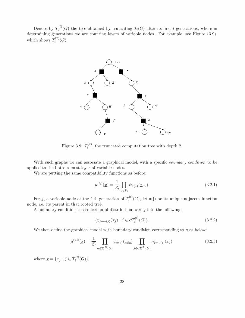
Denote by T(t)i (G) the tree obtained by truncating Ti(G) after its first t generations, where in

determining generations we are counting layers of variable nodes. For example, see Figure (3.9),

which shows T(2)i (G).

Figure 3.9: T(2)i , the truncated computation tree with depth 2.

With such graphs we can associate a graphical model, with a specific boundary condition to beapplied to the bottom-most layer of variable nodes.

We are putting the same compatibility functions as before:

µ(ti)(x) =1

Zt

∏

a∈Fi

ψπ(a)(x∂a). (3.2.1)

For j, a variable node at the t-th generation of T(t)i (G), let a(j) be its unique adjacent function

node, i.e. its parent in that rooted tree.A boundary condition is a collection of distribution over χ into the following:

{ηj→a(j)(xj) : j ∈ ∂T(t)i (G)}. (3.2.2)

We then define the graphical model with boundary condition corresponding to η as below:

µ(t,i)(x) =1

Zt

∏

a∈T(t)i (G)

ψπ(a)(x∂a)∏

j∈∂T(t)i (G)

ηj→a(j)(xj), (3.2.3)

where x = {xj : j ∈ T(t)i (G)}.

28

Proposition 3.2.1. Let ν(t)i (.) be the BP estimate for the marginals w.r.t µG(.) after t BP iterations

on G. If the boundary condition on T(t1)i (G) is taken to be ν

(t0)j→a(j)(.) = ηj→a(j)(.), then for t1 ≥ 1, t0 ≥

0 we haveν

(t0+t1)i (xi) = µ(t1,i)(xi), (3.2.4)

where µ(t1,i)(xi) is naturally the marginal corresponding to the root in T(t1)i (G) 1.

Proof. Let j be at level t1− s on Ti(G), a its parent, and call µT (j)j→a(xj) the marginal for xj w.r.t the

graphical model in the subtree T (j) (see figure 3.10). We prove by induction that

µT (j)j→a(xj) = ν

(t0+s)j→a (xj). (3.2.5)

Figure 3.10: The subtree rooted at j, namely T (j).

For s = 0 it is just a consequence of the choice of boundary conditions.If it is true for some s, assume that the level of j is t1− (s+1). Then by the induction hypothesis

we have the following (see figure 3.11).

µT (j)j→a(xj) ∝

∏

b∈∂j\a

∑

x∂b\j

ψb(x∂b)∏

l∈∂b\j

µT (j)l→b (xl)

∝∏

b∈∂j\a

∑

x∂b\j

ψb(x∂b)∏

l∈∂b\j

ν(t0+s)l→b (xl)

∝ ν(t0+s+1)j→a (xl). (3.2.6)

1Note that here one can see a slight abuse of notation, where we should use ηπ(j)→π(a(j)) instead of ηj→a(j) to becompletely accurate. We will use the simpler -though not very accurate form- in the rest of lecture.

29

Figure 3.11: used in proof of proposition 3.2.1

Now, repeat the same argument for the root and it completes the proof.

Corollary 3.2.2. If

supx(t),x(t)′

∣∣∣µ(t,i)(xi|x(t))− µ(t,i)(xi|x

(t)′)∣∣∣ ≤ δ(t) (3.2.7)

then, for any t1, t2 ≥ t we have ∣∣∣ν(t1)i (xi)− ν

(t2)i (xi)

∣∣∣ ≤ δ(t). (3.2.8)

In particular, if δ(t)→ 0 as t→∞, then belief propagation converges.

30

Proof. By the previous proposition we have:

∣∣∣ν(t1)i (xi)− ν

(t2)i (xi)

∣∣∣ =

=

∣∣∣∣∣∣

∑

x(t)

µ(t)(xi|x(t))ν

(t1−t)i (x(t))−

∑

x(t)

µ(t)(xi|x(t))ν

(t2−t)i (x(t))

∣∣∣∣∣∣

=

∣∣∣∣∣∣

∑

x(t),x(t)′

[µ(t)(xi|x

(t))− µ(t)(xi|x(t)′)]ν

(t1−t)i (x(t))ν

(t2−t)i (x(t)′)

∣∣∣∣∣∣

= δ(t). (3.2.9)

Now, let Bi(t) be the subgraph of G induced by the vertices whose distance from i is at most t.

Corollary 3.2.3. If Bi(t) is a tree and inequality 3.2.7 holds, then

∣∣∣∣∣∣∣µi(xi)︸ ︷︷ ︸

actual marginal

− ν(t)i (xi)︸ ︷︷ ︸

BP estimate

∣∣∣∣∣∣∣≤ δ(t). (3.2.10)

In particular, if g is the girth2 of G, then we will have

∣∣∣µi(xi)− ν(t)i (xi)

∣∣∣ ≤ δ(g − 1

2). (3.2.11)

Proof. Observe that

µi(xi) =∑

x(t)

µ(xi|x(t))µ(x(t)), (3.2.12)

where x(t) is the set of vertices at distance t from i in G. Also notice that µG(xi|x(t)) = µT (xi|x

(t)).Now, proceed as in the previous proof.

3.3 Dobrushin uniqueness criterion

In this section we consider a general factor graph model of the type (3.1.1) on the factor graphG = (V, F,E). We estabilish a general condition that is easy to check and implies correlationdecay. Applied to the computation tree, this approach allow to obtain sufficient conditions for theconvergence of belief propagation, and for its correctness on locally tree-like graphs.

The condition developed here was initially proposed by Roland Dobrushin in his study of Gibbsmeasures. While the initial results concerned traslation invariant models on regular grids, its gener-alization to arbitrary factor graphs is quite immediate. Dobrushin criterion measures the strengthof interactions as follows.

2The girth of an undirected graph G is defined by the length of the shortest cycle in it.

31

Definition 6. Given vertices i, j ∈ V , the influence of j on i is defined as

Cij = maxx,x′

{‖µ(xi = · |xV \i)− µ(xi = · |x′V \i)‖TV : xl = x′x ∀l 6= j

}

Notice that by definition 0 ≤ Cij ≤ 1 and Cij = 0 unless d(i, j) = 1 (i.e. unless i, j are neighborsof the same factor node). The following theorem shows that small influence implies correlation decay.Here, for a vertex i, we let Bi(t) denote the ball of radius t around i, and Bi(t) its complement.

Theorem 3.3.1 (Dobrushin, 1968). Assume

γ ≡ supi∈V

( ∑

j∈V \i

Cij

).

Then for any i ∈ V , any t ≥ 0, letting B = Bi(t), we have

maxx,x′‖µ(xi = · |x

B)− µ(xi = · |x′

B)‖TV ≤

γt

1− γ.

In other words, this theorem estabilishes that correlations decay exponential in the graph distancewith a rate that is controlled by the parameter γ defined in the statement.

Proof. With a slight abuse of notation, let us denote by µ, µ′ the conditional measure on xBi(t) given

configurations xB, x′

Bon Bi(t). We will construct a coupling µ of µ, µ′ such that

µ(xi 6= x′i) ≤γt

1− γ.

This coupling can be constructed recursively as follows:

1: Start from µ = µ× µ′.

2: Repeat

(a) Choose j ∈ Bi(t);

(b) Define a new coupling µnew as follows:

(b1) Sample x, x′ ∼ µ;

(b2) Resample (xj , x′j) from the optimal coupling

between µ(xj |xV \j) and µ(xj |x′V \j);

(c) Let µ← µnew;

The vertex j in step (a) is selected in such a way that the vertices in Bi(t) are swept over.The proof consists in analyzing this recursion. Let µ(k) be the coupling produced after k sweeps,

and assume we are given numbers a(k)j such that for all j ∈ Bi(t)

µ(k)(xj 6= x′j) ≤ a(k)j .

Then it is easy to show that at the next iteration analogous upper bounds can be obtained by letting

a(k+1)j =

∑

l∈V \j

Cjla(k)l , (3.3.1)

where a(k)l = 1 by definition for l ∈ Bi(t). The thesis follows by controlling the recursion (3.3.1). [A

few more details to be written.]

32

Chapter 4

Variational methods

The basic idea in variational approaches to formulate the inference problem as an optimizationproblem. Once this is done, all sorts of ideas from standard optimization theory can be appliedto solve or approximately solve the optimization problem. It turns out that the whole approach isparticularly simple and clean when (guess what) the inference problem was an optimization problemto start with, e.g. in the mode computation.

The whole idea of connecting inference (more precisely, computation of expected values of high-dimensional probability distributions) to optimization dates back to physics. It is a known fact inthermodynamics that systems in thermal equilibrium with their environment tend to optimize theirfree energy. A mathematical foundation for this physical law was provided by statistical mechanicswith Gibbs’ variational principle. The implications of these ideas to algorithms and graphical modelswhere first discussed by Yedidia and coworkers [YFW05], and subsequently extended in a number ofways (see for instance [WJW05] and the review [WJ08]).

This chapter is organized as follows. The basic connection between inference and optimizationis introduced in Section 4.1. One basic way to use this connection is the so-called naive mean fieldapproximation, discussed in Section 4.2. We then develop Bethe approximation to the Gibbs freeenergy and show its connection to belief propagation in Section 4.3. Finally, we explain two waysof modifying Bethe approximation, namely region-based approximations in Sections 4.4 and 4.6,together with the algorithms based on these approximations.

4.1 Free Energy and Gibbs Free Energy

Throughout this chapter we shall use the graphical model formalism and hence assume that a model(G,ψ) is given, with G = (V, F,E) a factor graph and ψ = {ψa}a∈F a collection of compatibilityfunctions. We define the joint distribution as

µ(x) =1

Z

∏

a∈F

ψa(x∂a) .

The concepts discussed in this section do not depend on the factorization of µ accordinbg to G butonly on the total weight ψ(x) ≡

∏a∈F ψa(x∂a) We will therefore consider a generic un-normalized

weigth ψ : X V → R+, and use this weight to compute a probability distribution

µ(x) =1

Zψ(x) . (4.1.1)

33

We begin define the Helmotz free energy and Gibbs free energy of a distribution.

Definition 7 (Helmotz Free Energy). Given a model (G,ψ), its Helmotz free energy is defined as

Φ = logZ = log{∑

x

∏

a∈F

ψa(x∂a)}.

A few remarks are in order. First of all, physicists normally call ‘free energy’ the quantity1

− logZ, but the minus sign is usually misterious for non-physicists and we will therefore drop it.Second, the ‘Helmotz’ qualifier is not that common. We will drop it most of the times. Sometimes,the same quantity is called mor simply log-partition function.

The importance of Φ can be understood by recalling that computing marginals of µ is equivalentto computing differences Φ − Φ′ for modified models. Also sampling from µ can be reduced tocomputing Φ for a sequence of models.

We next introduce the notion of Gibbs free energy. Again, the factorization structure is notcrucial here, but we can consider any model of the form (4.1.1). (Recall that H(p) is Shannon’sentropy of the distribution p.)

Definition 8 (Gibbs free energy). Given a model (G,ψ), its Gibbs free energy is a function G :

M(X V )→ R. For a distribution ν ∈ M(X V ), the corresponding Gibbs free energy is defined as

G(ν) = H(ν) + Eν logψ(x) (4.1.2)

= −∑

x

ν(x) log ν(x) +∑

x

ν(x) logψ(x) . (4.1.3)

The connection between these concepts is provided by the following result.

Proposition 4.1.1. The function G : M(X V )→ R is strictly concave on the convex domain M(X V ).Further its unique maximum is achieved at ν = µ, with G(µ) = Φ.

Proof. Convexity is just a consequence of the fact that z 7→ z log z is convex on R+. The uniqueminimum can be found by introducing the Lagrangian

L(ν, λ) = G(ν)− λ

(∑

x

ν(x)− 1

). (4.1.4)

Setting to zero the derivative with respect to ν(x), one gets ν(x) = ψ(x)/Z. It is immediate to checkthat the value at the minimum is indeed Φ.

Remark 2. Gibbs free energy can be re-expressed as follows:

G[ν] = Φ−D(ν||µ)

where D( · ) is the Kullback-Leibler divergence between ν and µ [CT91].

1More precisely, they call free enregy the quantity −(Temp.) × log Z with Temp. the system temperature.

34

We therefore reformulated the inference problem as a convex optimization problem, and we knowthat convex optimization is tractable! The problem of course is that the search space is very high-dimensional. The dimension of M(X V ) is (|X |n − 1) which scales exponentially in the model size.For reasonably large models even storing such a vector is impossible.

The basic idea of variational inference is look for approximate solutions of this problem. Thefollowing tricks are at the core of most approach: (i) Optimize G(ν) only within a low-dimensionalsubset of M(X V ); (ii) Construct low-dimensional projections of M(X V ), and approximate G(ν) at apoint ν by some function of the projection.

4.2 Naive mean field

Naive mean field amounts to applying trick (i) in the above list, whereby the subset is just the setof measure of product form, i.e. such that

ν(x) =∏

i∈V

νi(xi) . (4.2.1)

If we write ν = (ν1, ν2, . . . , νn) ∈ M(X )×· · ·×M(X ) ≡ M(X )V for a vector of one-variable marginals,we can denote formally the above embedding of factorized distributions into M(X V ), K : M(X )V →M(X V ), by

K(ν)(x) =∏

i∈V

νi(xi) . (4.2.2)

The Naive Mean Field free energy is then the function GMF : M(X )V → M(X V ) defined by

GMF(ν) = G(K(ν)) . (4.2.3)

Plugging this in the definition of Gibbs free energy , we obtain the following explicit expression:

GMF(ν) = H(K(ν)) + Eν[logψ(x)]

=∑

i∈V

H(νi) +∑

a∈F

∑

x∂a

∏

i∈∂a

νi(xi) logψa(x∂a) .

It is an immediate consequence of Proposition 4.1.1 that the naive mean field approximation providesa lower bound on the free energy, namely

Φ ≥ maxν∈M(X )V

GMF(ν) (4.2.4)

The nice fact about this expression is that the resulting optimization problem has much lower di-mensionality than for Gibbs variational principle: we passed from (|X |n−1) to n(|X |−1). The priceto pay is that GMF is no longer a concave function and therefore solving the optimization problemcan be hard.

It is instructive to write down the stationarity conditions for GMF. We introduce Lagrangemultipliers λi to constrain the beliefs νi to be normalized, that is,

∑xiνi(xi) = 1, giving us the

35

following Lagrangian and derivatives:

L(ν, λ) =∑

i∈V

H(νi) +∑

a∈F

∑

x∂a

∏

i∈∂a

νi(xi) logψa(x∂a) +∑

i∈V

λi

(∑

xi

νi(xi)− 1

),

∂L

∂νi(xi)= −1− log νi(xi) +

∑

a∈∂i

∑

xj :j∈∂a\i

∏

j∈∂a\i

νj(xj) logψa(x∂a) + λi .

Solving, we obtain the stationarity conditions

νi(xi) = exp

∑

a∈∂i

∑

xj :j∈∂a\i

∏

j∈∂a\i

νj(xj) logψa(x∂a) + λi − 1

∼= exp

∑

a∈∂i

∑

xj :j∈∂a\i

logψa(x∂a)∏

j∈∂a\i

νj(xj)

(4.2.5)

where we solved for λi to normalize the ν’s. These are somewhat more transparent if we introducemessages νa→i(xi) thus getting the following equations

νi(xi) ∼=∏

a∈∂i

νa→i(xi) , (4.2.6)

νa→i(xi) ∼= exp

∑

xj :j∈∂a\i

logψa(x∂a)∏

j∈∂a\i

νj(xj)

. (4.2.7)

A simple greedy algorithm for finding a stationary point consists in updating the ν’s by iterating theabove equations until convergence. Of course, standard first orded methods can be used as well toreach a stationary point of GMF.

4.2.1 Pairwise graphical models and the Ising model

Consider the special case of a pairwise model

µ(x) =1

Z

∏

(i,j)∈E

ψij(xi, xj)∏

i∈V

ψi(xi) . (4.2.8)

Then the naive mean field equations read

νi(xi) ∼= ψi(xi) exp

∑

j∈∂i

∑

xj

logψij(xi, xj)νj(xj)

. (4.2.9)

As an example we will consider again Ising models, which we recall are pairwise graphical modelswith binary variables xi ∈ X = {+1,−1}. For the sake of simplicity we shall assume G to bea d-dimensional discrete torus of linear size L. This is obtained by letting the vertex set be V ={1, . . . , L}d ⊆ Z

d, and the edge set (i, j) ∈ E if and only if j = (i±ek) mod L where ek, k = 1, . . . , dis the canonical basis. This graph is reproduced in Fig. ??, for d = 2 dimensions.

36

To have complete symmery among vertices, we also assume that potentials are all equal and thatthey are symmetric ander change of sign of the variables, i.e.

ψij(xi, xj) = eβxixj , i.e. ψij =

(eβ e−β

e−β eβ

). (4.2.10)

This defines the joint probability distribution

µ(x) =1

Zexp

{β∑

(i,j)∈E

xi, xj

}. (4.2.11)

The mean field free energy takes the form

GMF(ν) =∑

i∈V

H(νi) + β∑

(i,j)∈E

∑

xixj

νi(xi)νj(xj)xixj . (4.2.12)

Since variables are binary, a single real number is sufficient to pearametrize each marginal. We chosethis number to be the expectation:

νi(xi) =1 +mixi

2, Eνi

[xi] = mi .

We have of course mi ∈ [−1,+1]. By substituting in Eq. (4.2.12), we get the explicit expression(with some abuse of notation)

GMF(m) = =∑

i∈V

h((1 +mi)/2

)+ β

∑

(i,j)∈Γ

mimj .

where h(x) ≡ −x log x− (1− x) log(1− x).The mean field equationtion (4.2.9) reduces to

νi(xi) ∼= exp{β∑

j∈∂i

xi

∑

xj

νj(xj)xj

}(4.2.13)

and we thus have the fllowing equations for the means

mi =exp

(β∑

j∈Γ(i)mj

)− exp

(−β∑

j∈Γ(i)mj

)

exp(β∑

j∈Γ(i)mj

)+ exp

(−β∑

j∈Γ(i)mj

)

= tanh

β

∑

j∈Γ(i)

mj

. (4.2.14)

Recall the hyperbolic tangent is a strictly increasing function bounded by [−1, 1].

37

Convergence of iterative mean field updates for Ising models

In this section, we will be considering the convergence properties of the iterative updates we havederived for our mean-field approximation of Ising models. More precisely, we shall consider theiteration

m(t+1)i = tanh

β

∑

j∈∂i

m(t)j

. (4.2.15)

It turns that this iteration always converges if a uniform initialization is used. On the other hand,the accuracy of the result depends strongly on the strength of interactions which is tuned via theparameter β.

First, it follows from Eq. (4.2.15) that, if we initialize m(0)i = m(0) for all i ∈ V , we will have

m(t)i = m(t) for all t ≥ 0. This common value evolves according to the one-dimensional recursion

m(t+1) = tanh(2dβm(t)

). (4.2.16)

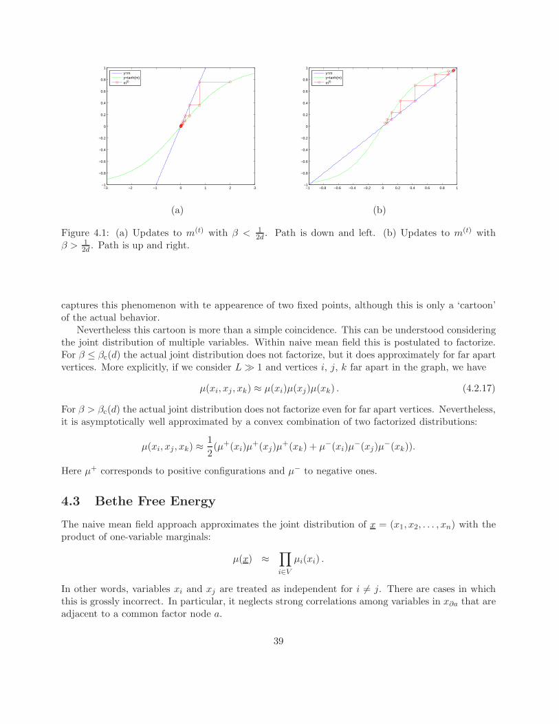
This recursion can be easily studied graphically, cf. Fig. 4.1. The function x 7→ tanh(x) is odd andhas maximum derivative at x = 0, where tanh(x) = x + O(x3). Hence for β < 1

2d , the slope of themapping in Eq. (4.2.16) is everywhere smaller than 1, and therefore the mapping is a contraction.No matter the value of m(0), the iterations will converge to limt→∞m(t) = 0. An illustration of thisis in Fig. 4.1(a).

If β > 12d , on the other hand, the slope of the hyperbolic tangent will be greater than 1 at m = 0,

and there are three points that the line y = m will intersect y = tanh (β∑m). Thus, if we begin the

iterations with m(0) > 0, limt→∞m(t)i = +m∗. If m(0) < 0, then the iterations will converge to −m∗,

and in the degenerate case that m(0) = 0, we will converge to the saddlepoint 0. An illustartion ofthis is in Fig. 4.1(b).

Marginals in the Ising Model

Up ot this point, we have ignored the marginals of the actual distribution of the Ising model, fo-cusing instead on the partition function and maximizing the free energy. Is the naive mean fieldapproximation reproducing the correct marginals.

It is easy to see that the real marginals µi(xi) should be uniform i.e. µi(+1) = µi(−1) = 1/2,because the factors are completely symmetric under exchange of signs of the variables x. In otherwords for each configuration x, te flipped configuration −x has exactly the same probability under µ.This apperars to be captured by the naive mean field approximation only for ‘weak’ factors, namelyfor β ≤ 1/(2d).

For β > 1/(2d), the fixed point m = 0 becomes unstable, and the mean field iteration convergesto the either of the fixed points m = ±m∗. This appears at first sight completely incorrect, andjust a pathology of the naive mean field approximation. In fact this is not the hole story. At largeenough β, we have that the model is equally likely to have most of its variables either +1 or −1. Thedistribution µ becomes strongly bimodal. This can be revealed for instance by considering the sumof variables

∑i∈V xi. For d ≥ 2 and any β > βrmc(d) the distribution of this quantity concentrates

around values ±m0|V | as L→∞. This is a typical ‘phase transition’ phenomenon. Naive mean field

38

−3 −2 −1 0 1 2 3−1

−0.8

−0.6

−0.4

−0.2

0

0.2

0.4

0.6

0.8

1y=my=tanh(m)

m(i)

−1 −0.8 −0.6 −0.4 −0.2 0 0.2 0.4 0.6 0.8 1−1

−0.8

−0.6

−0.4

−0.2

0

0.2

0.4

0.6

0.8

1y=my=tanh(m)

m(i)

(a) (b)

Figure 4.1: (a) Updates to m(t) with β < 12d . Path is down and left. (b) Updates to m(t) with

β > 12d . Path is up and right.

captures this phenomenon with te appearence of two fixed points, although this is only a ‘cartoon’of the actual behavior.

Nevertheless this cartoon is more than a simple coincidence. This can be understood consideringthe joint distribution of multiple variables. Within naive mean field this is postulated to factorize.For β ≤ βc(d) the actual joint distribution does not factorize, but it does approximately for far apartvertices. More explicitly, if we consider L≫ 1 and vertices i, j, k far apart in the graph, we have

µ(xi, xj , xk) ≈ µ(xi)µ(xj)µ(xk) . (4.2.17)

For β > βc(d) the actual joint distribution does not factorize even for far apart vertices. Nevertheless,it is asymptotically well approximated by a convex combination of two factorized distributions:

µ(xi, xj , xk) ≈1

2(µ+(xi)µ

+(xj)µ+(xk) + µ−(xi)µ

−(xj)µ−(xk)).

Here µ+ corresponds to positive configurations and µ− to negative ones.

4.3 Bethe Free Energy

The naive mean field approach approximates the joint distribution of x = (x1, x2, . . . , xn) with theproduct of one-variable marginals:

µ(x) ≈∏

i∈V

µi(xi) .

In other words, variables xi and xj are treated as independent for i 6= j. There are cases in whichthis is grossly incorrect. In particular, it neglects strong correlations among variables in x∂a that areadjacent to a common factor node a.

39

As an example, consider the graphical model with a single factor node a and three variables x1,x2, x3 ∈ {0, 1}, whose joint distribution is given by

µ(x1, x2, x3) =1

ZI(x1 ⊕ x2 ⊕ x3 = 0) .

Here ⊕ denotes sum modulo 2, and we obviously have Z = 4. It is a simple exercise to show thatthe naive mean field yields the disappointing estimate ZMF = 1.

Bethe-Peierls approximation improves in a crucial way, by accounting for correlations induced byfactor nodes. Instead of parametrizing the entire distribution in terms of single variable marginalsµi(xi). Bethe-Peierls approximation instead keeps track of joint distributions µa(xa). We will startby building intuition in the case of tree factor graphs, then define the Bethe free energy in the caseof general graphs, and finally discuss the connection with belief propagation.

4.3.1 The case of tree factor graphs

The variational approximation we are going to construct will approximate the Gibbs free energyas a function of single variable marginals µi(xi), and of joint distributions at a factor node µa(xa).Valuable insight can be gained by considering the case of tree factor graphs. In this case we havethe following important structural result.

Lemma 4.3.1. If (G,ψ) is a tree factor graph model, then the corresponding joint distribution µ isgiven by

µ(x) =∏

a∈F

(µa(x∂a)∏i∈∂a µi(xi)

)∏

i∈V

µi(xi) (4.3.1)

=∏

a∈F

µa(x∂a)∏

i∈V

µi(xi)1−|∂i| .

Proof. The proof will proceed by induction on |F |. For the base case, assume |F | = 0. The expression(4.3.1) then reduces to µ(x) =

∏i∈V µi(xi) which is correct, since for an empty factor graph the

variables x1, . . . , xn are independent.Now assume that the claim holds for all tree graphs such that |F | ≤ m. We need to now check

the expression (4.3.1) for |F | = m+ 1. Consider a tree G with m factor nodes, and at variable nodei, we append a factor node a (along with other variable nodes connected to a), to get a tree G′ withm + 1 factor nodes. Indeed any graph G′ eith m + 1 factor nodes can be decomposed in this way,see Fig. 4.2.

Note that |∂i| is the number of factor nodes connected to variable node i in graphG′. Thus numberof factor nodes connected to i in graph G is |∂i| − 1. Further notice that the joint distribution of thevariables in V , factors according to the graph G. We therefore have, by the induction hypothesis,

µ(xV ) =∏

b∈G

µb(x∂b)∏

j∈G\i

µj(xj)1−|∂j|µi(xi)

1−(|∂i|−1) .

By Bayes rule µ(xV ′) = µ(xV )µ(x∂a\i|xV ). On the other hand the vertex i separates ∂a \ i fromV \ {i}. By the global Markov property we have

µ(x∂a\i|xV ) = µ(x∂a\i|xi) .

40

Figure 4.2: Addition of a single factor node to graph G

Using therefore the induction hypothesis we get

µ(xV ′) = µ(xV )µ(x∂a\i|xi)

=∏

b∈G

µb(x∂b)∏

j∈G\i

µj(xj)1−|∂j|µi(xi)

1−(|∂i|−1)µ(x∂a\i, xi)

µi(xi)

=∏

b∈G′

µb(x∂b)∏

j∈G′

µj(xj)1−|∂j| ,

where the last equality follows from the fact that µ(x∂a\i, xi) = µa(x∂a) and for variable nodesj ∈ ∂a \ i the number of neighbouring factor nodes |∂j| = 1. This completes the induction step,thereby proving the lemma.

As an example, consider a Markov chain. The expression for the distribution now reduces to

µ(x) =n−1∏

a=1

µa(xa, xa+1)n−1∏

i=2

µi(xi)−1

= µ1(x1, x2)n−1∏

i=2

µi(xi, xi+1)

µi(xi)

= µ1(x1)µ1(x2|x1)

n−1∏

i=2

µi(xi+1|xi)

= µ1(x1)

n−1∏

i=1

µi(xi+1|xi)

Thus we obtain the usual formula for the distribution of a Markov Chain.

41

Calculating the Gibbs energy for trees, one obtains,

G(µ) = H(µ) +∑

a∈F

Eµ log(ψa(x))

= −∑

x

µ(x) log µ(x) +∑

a∈F

∑

x∂a

µa(x∂a) logψa(x∂a)

= −∑

x

µ(x) log

(∏

a∈F

µa(x∂a)∏

i∈V

µi(xi)1−|∂i|

)+∑

a∈F

∑

x∂a

µa(x∂a) logψa(x∂a))

= −∑

a∈F

∑

x∂a

µa(x∂a) log µa(x∂a)−∑

i∈V

∑

xi

(1− |∂i|)µi(xi) log µi(xi) +∑

a∈F

∑

x∂a

µa(x∂a) logψa(x∂a)

=∑

a∈F

H(µa)−∑

i∈V

(|∂i| − 1)H(µi) +∑

a∈F

∑

x∂a

µa(x∂a) logψa(x∂a)

Here H( · ) is the Shannon entropy. We therefore proved the following.

Corollary 4.3.2. If (G,ψ) is a tree factor graph model, then the corresponding Gibbs free energy is

G(µ) =∑

a∈F

H(µa)−∑

i∈V

(|∂i| − 1)H(µi) +∑

a∈F

∑

x∂a

µa(x∂a) logψa(x∂a)

4.3.2 General graphs and locally consistent marginals

For the general case, one can have marginals {bi, ba} for each factor node a ∈ F and variable nodei ∈ V , which define the Gibbs free energy. We see that such marginals have to satisfy the followingconditions to be a valid set of marginals.

bi(xi) ≥ 0, ∀xi, ∀i ∈ V

ba(x∂a) ≥ 0, ∀x∂a, ∀a ∈ F (4.3.2)∑

xi

bi(xi) = 1, ∀i ∈ V (4.3.3)

∑

x∂a\i

ba(x∂a) = bi(xi), ∀a ∈ F, i ∈ ∂a (4.3.4)

∑

x∂a

ba(x∂a) = 1, ∀a ∈ F. (4.3.5)

Note that Eqn(4.3.3) and Eqn(4.3.4) imply Eqn(4.3.5), and hence we can remove that equation fromthe requirements of a valid marginal.

The set of marginals {bi, ba} on a graph G which satisfy the above requirements is known as theset of locally consistent marginals on G, denoted by LOC(G). As the above constraints are linear, itcan be readily seen that the set LOC(G) is a convex set. Also the dimension of LOC(G) is boundedabove by |X |max |∂a||F |.

We will now contrast the set of locally consistent marginals LOC(G) for the cases when G is atree and when G is not.

42

• G is a Tree

– When G is a tree, then for any {bi, ba} ∈ LOC(G), there exists an unique measureb∗ ∈Measures(X ν) whose marginals are given by {bi, ba}.

– The measure b∗ is given by

b∗(x) =∏

a∈F

(ba(x∂a)∏i∈∂a bi(xi)

)∏

i∈V

bi(xi)

– The Gibbs free energy for b∗ is given by G(b∗) = G(ba, bi) and hence logZ = maxLOC(G) G(ba, bi)

• G is not a Tree

– In this case, there exists a set of marginals {bi, ba} ∈ LOC(G) that are not marginals ofany distribution b on the graph G.

The example of a case where the set {bi, ba} ∈ LOC(G) fails to be the marginals for any dis-tribution on G, can be obtained by considering the case of cyclic graph consisting of three variablenodes and three factor nodes as in Fig(??). Each variable xi takes values in the set {0, 1}. Thecompatibility function for each factor node is specified in the matrix form as,

b12 =

[0.49 0.010.01 0.49

]b23 =

[0.49 0.010.01 0.49

]b13 =

[0.01 0.490.49 0.01

]

From the compatibility function matrices, one observes that the factor node (1, 2) prefers that variablenodes 1 and 2 be in the same state. Similarly factor node (2, 3) prefers that variable nodes 2 and3 be in the same state. On the other hand, factor node (1, 3) prefers variable nodes 1 and 3 be indifferent states. It follows that not all of the compatibility functions can be satisfied simultaneouslyby a distribution. On the other hand, it can be readily checked that the marginals defined bybi(xi) = (0.5, 0.5) and bij = ψij are locally consistent. The relation between the set of marginals ofsome distribution on G and the set LOC(G) is summed up in Fig(??)

The following two results describe the relationship between the stationary points of Gibbs freeenergy on the set LOC(G) and the fixed point of the Belief Propagation Algorithm on G and thusthe relationship between the Gibbs free energy and Bethe free energy.

Proposition 4.3.3. If the compatibility functions of a factor graph G are such that ψa(x∂a) > 0 forall x∂a and a ∈ F , then there exists a stationary point of G(bi, ba) in the interior of LOC(G). Inthis case, there exists a fixed point of the Belief Propagation Algorithm on G, which is given by theabove stationary point.

Claim 4.3.4. The Bethe free energy is the Lagrangian dual of the Gibbs free energy for the locallyconsistent marginals .

Proof. Before writing the Lagrangian dual for the Gibbs free energy on the set LOC(G), note thatthe constraints are specified by Eqn(4.3.3) and Eqn(4.3.4). Thus, in the dual, there will be a variableλi for each variable node i ∈ V , and a variable λi→a(xi) for all xi and for each edge (ia) ∈ G. Thusthe Lagrangian dual is given by

L({b}, {λ}) = G(b)−∑

i

λi

(∑

xi

bi(xi)− 1

)−∑

(ia)

∑

xi

λi→a(xi)

∑

x∂a\i

ba(x∂a)− bi(xi)

43

Setting ∂L∂b = 0 leads to an expression of b as a function of λ. Substituting this into the above

expression, one gets L as a function of just λ, which after a variable change from λ to {νi→a, νa→i}leads to the expression for Bethe Free energy.

Last lecture we saw that the Bethe free energy is the Lagrange dual of the Gibbs free energy forthe locally consistent marginals. Given a set of messages {νa→i, νi→a} we can construct the marginalsby setting ∂L

∂b = 0

bi(xi) ∝∏

a∈∂i

νa→i(xi)

ba(x∂a) ∝ ψa(x∂a)∏

i∈∂a

νi→a(xi)

Now by imposing the locally consistency condition we get the belief propagation fixed points. Let

νi→a(xi) ∝∏

b∈∂i\a

νa→i(xi)

Imposing the locally consistency condition∑

x∂a\iba(x∂a) = bi(xi), we get

∏

b∈∂i

νb→i(xi) ∝∑

x∂a\i

ψ(x∂a)∏

j∈∂a

νj→a(xj)

νa→i(xi)∏

b∈∂i\a

νb→i(xi) ∝∑

x∂a\i

ψ(x∂a)νi→a(xi)∏

j∈∂a\i

νj→a(xj)

νa→i(xi) ∝∑

x∂a\i

ψ(x∂a)∏

j∈∂a\i

νj→a(xj)

4.3.3 Bethe free energy as a functional over messages

Recall the definition of the Bethe Free Energy GB : {ν, ν} → R as

GB(ν, ν) = −∑

i,a

log

(∑

xi

νi→a(xi)νa→i(xi)

)+∑

a∈F

log

∑

x∂a

ψa(x∂a)∏

i∈∂a

νi→a(xi)

+∑

i∈V

log

(∑

xi

∏

a∈∂i

νa→i(xi)

).

Note that there are three terms in the expression, one for each edge, one for each factor node, andone for each variable node in the factor graph. The following claim justifies the study of Bethe freeenergy.

Proposition 4.3.5. For any factor graph, the stationary points of the Bethe free energy correspondto the fixed points of the Belief Propagation algorithm and vice versa. That is,

∂GB

∂ν= 0

if and only if the messages are a fixed point of belief propagation.

44

Proof. Note first from the definition of the Bethe free energy, that it is independent of scale withrespect to each of its arguments. That is, if we replace, νi→a(xi) by λνi→a(xi) for some λ > 0, thenthe value of the Bethe free energy remains the same. Differentiating the expression for the BetheFree energy with respect to νi→a(xi), we get

∂GB

∂νi→a(xi)= −

νa→i(xi)∑xiνi→a(xi)νa→i(xi)

+

∑x∂a\i

ψa(x∂a)∏

j∈∂a\i νj→a(xj)∑

x∂aψa(x∂a)

∏j∈∂a νj→a(xj)

Setting ∂GB∂νi→a(xi)

= 0 and rearranging the expression we see that,

νa→i(xi) =

( ∑xiνi→a(xi)νa→i(xi)∑

x∂aψa(x∂a)

∏j∈∂a νj→a(xj)

)∑

x∂a\i

ψa(x∂a)∏

j∈∂a\i

νj→a(xj)

∝∑

x∂a\i

ψa(x∂a)∏

j∈∂a\i

νj→a(xj)

which is nothing but the equation for the fixed point of the Belief propagation algorithm (for factormessage). The corresponding equation for the variable message can be obtained similarly by differ-entiating the expression for Bethe Free energy with respect to νa→i(xi) and setting ∂G

∂νa→i(xi)= 0.

Doing this we get,

νi→a(xi) ∝∏

b∈∂i\a

νb→i(xi)

Thus the stationary points of the Bethe free energy are the fixed points for the Belief Propagationalgorithm. The converse can be obtained by direct substitution.

4.4 Region-Based Approximation of the Free Energy

The idea of this approximation is that we have a complicated system for which we cannot computethe free energy. Therefore, We decompose the system into subsystems and then approximate thefree energy by combining the free energies of the subsystems.

4.4.1 Regions and Region-Based Free Energy

We define a region R of a factor graph G = (V, F,E) to be (VR, FR, ER) such that

a ∈ FR ⇒ ∂a ⊆ VR

i ∈ VR, a ∈ FR, (i, a) ∈ E ⇒ (i, a) ∈ ER

An example of a region is shown in Figure 4.3 (a). Given a region R, the Gibbs free energy of theregion GR : M(X VR)→ R is

GR[bR] = H[bR] +∑

xR

∑

a∈FR

bR(xR) log(ψa(x∂a)) = HR[bR]− UR[bR]

45

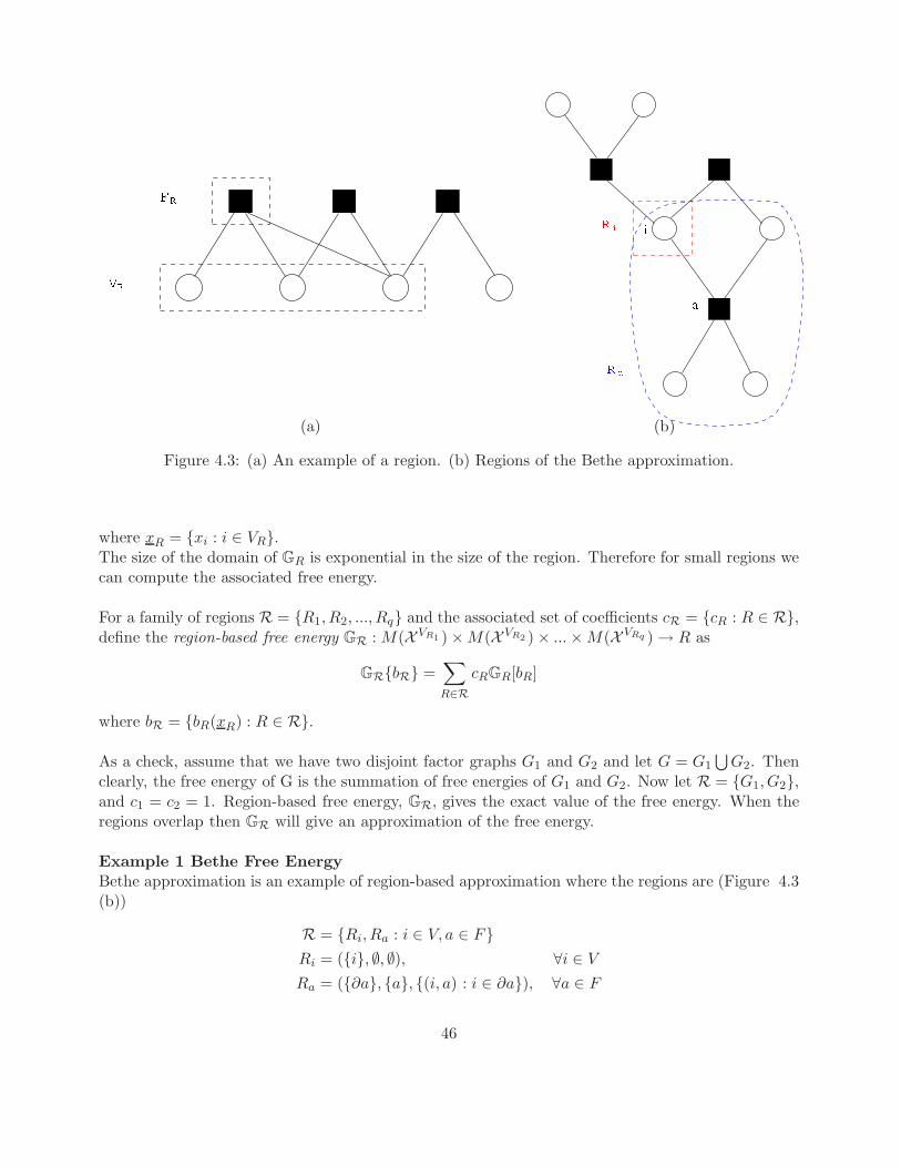
(a) (b)

Figure 4.3: (a) An example of a region. (b) Regions of the Bethe approximation.

where xR = {xi : i ∈ VR}.The size of the domain of GR is exponential in the size of the region. Therefore for small regions wecan compute the associated free energy.

For a family of regions R = {R1, R2, ..., Rq} and the associated set of coefficients cR = {cR : R ∈ R},define the region-based free energy GR : M(X VR1 )×M(X VR2 )× ...×M(X VRq )→ R as

GR{bR} =∑

R∈R

cRGR[bR]

where bR = {bR(xR) : R ∈ R}.

As a check, assume that we have two disjoint factor graphs G1 and G2 and let G = G1⋃G2. Then

clearly, the free energy of G is the summation of free energies of G1 and G2. Now let R = {G1, G2},and c1 = c2 = 1. Region-based free energy, GR, gives the exact value of the free energy. When theregions overlap then GR will give an approximation of the free energy.

Example 1 Bethe Free EnergyBethe approximation is an example of region-based approximation where the regions are (Figure 4.3(b))

R = {Ri, Ra : i ∈ V, a ∈ F}

Ri = ({i}, ∅, ∅), ∀i ∈ V

Ra = ({∂a}, {a}, {(i, a) : i ∈ ∂a}), ∀a ∈ F

46

and the coefficients are

ci = 1− |∂i|, ∀i ∈ V

ca = 1, ∀a ∈ F

The corresponding region-based free energy is

GR{ba, bi} =∑

i∈V

(1− |∂i|)H[bi] +∑

a∈F

H[ba] +

∑

x∂a

ba(x∂a) log(ψa(x∂a))

4.4.2 Region-Based Approximation

We approximate the free energy by

F = log(Z) ≈ maxbR

GR{bR}

where the marginals of the regions must be consistent, i.e.

∀R ⊃ R′ :∑

xR\R′

bR(xR) = bR′(xR′)

and the coefficients must satisfy the following rules

∑

R∈R

cRI(i ∈ VR) = 1, ∀i ∈ V (4.4.1)

∑

R∈R

cRI(a ∈ FR) = 1, ∀a ∈ F (4.4.2)

Constraining the coefficients to satisfy rules (4.4.1) and (4.4.2) has the following consequences

1. If (4.4.2) holds and the marginals {bR : R ∈ R} are the real marginals then UR(bR) is equal tothe energy term of the Gibbs free energy of the real distribution, i.e, U [µ] = −Eµ log(ψ(x)).

UR(bR) = −∑

R∈R

cR∑

xR

bR(xR)∑

a∈FR

ψa(x∂a)

= −∑

R∈R

∑

a∈F

I(a ∈ FR)cR∑

x∂a

µa(x∂a)ψa(x∂a)

= −∑

a∈F

(∑

R∈R

I(a ∈ FR)cR

)∑

x∂a

µa(x∂a)ψa(x∂a)

= −∑

a∈F

∑

x∂a

µa(x∂a)ψa(x∂a)

= U [µ]

2. If (4.4.1) holds, the marginals {bR : R ∈ R} are the real marginals, and the real distributionis uniform then HR(bR) is equal to the entropy term of the Gibbs free energy of the realdistribution.

47

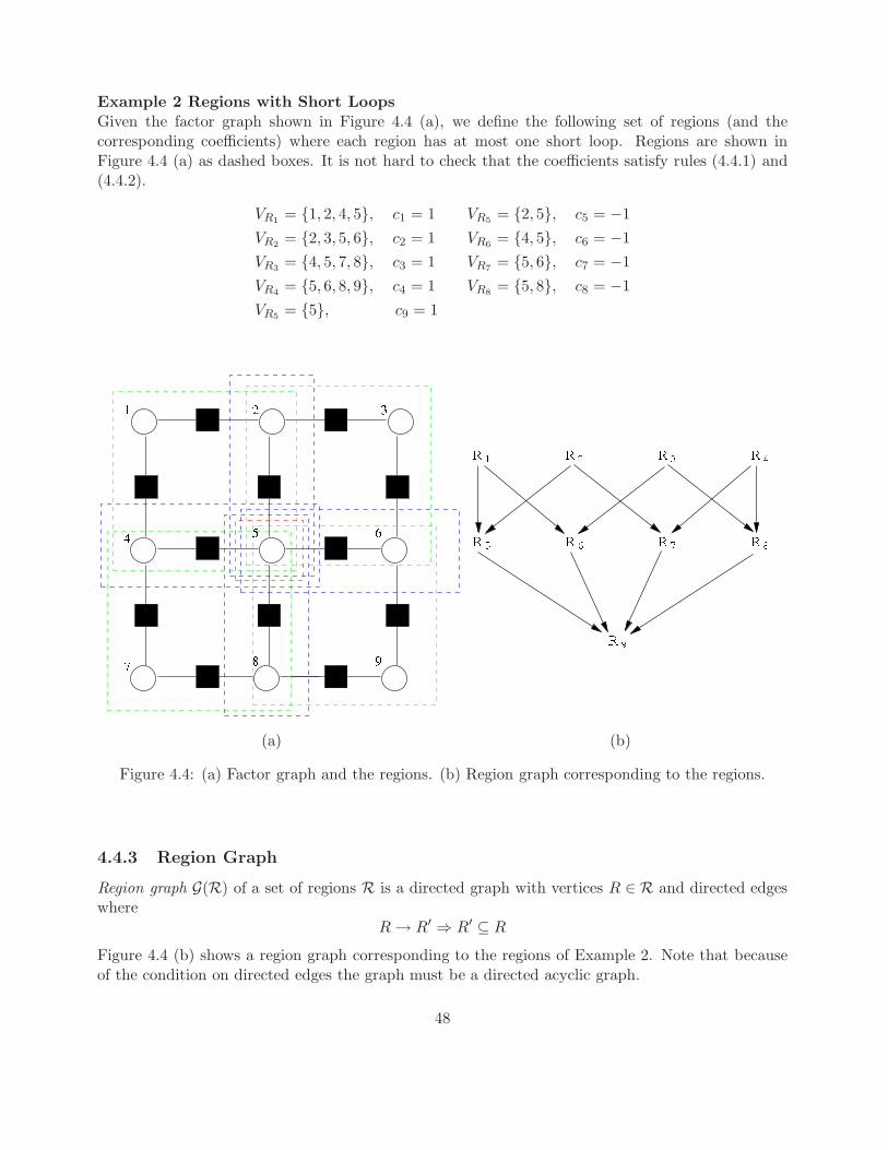
Example 2 Regions with Short LoopsGiven the factor graph shown in Figure 4.4 (a), we define the following set of regions (and thecorresponding coefficients) where each region has at most one short loop. Regions are shown inFigure 4.4 (a) as dashed boxes. It is not hard to check that the coefficients satisfy rules (4.4.1) and(4.4.2).

VR1 = {1, 2, 4, 5}, c1 = 1 VR5 = {2, 5}, c5 = −1

VR2 = {2, 3, 5, 6}, c2 = 1 VR6 = {4, 5}, c6 = −1

VR3 = {4, 5, 7, 8}, c3 = 1 VR7 = {5, 6}, c7 = −1

VR4 = {5, 6, 8, 9}, c4 = 1 VR8 = {5, 8}, c8 = −1

VR5 = {5}, c9 = 1

(a) (b)

Figure 4.4: (a) Factor graph and the regions. (b) Region graph corresponding to the regions.

4.4.3 Region Graph

Region graph G(R) of a set of regions R is a directed graph with vertices R ∈ R and directed edgeswhere

R→ R′ ⇒ R′ ⊆ R

Figure 4.4 (b) shows a region graph corresponding to the regions of Example 2. Note that becauseof the condition on directed edges the graph must be a directed acyclic graph.

48

If there is a directed edge between R and R′ then we say that R is a parent of R′, R ∈ P (R′),and R′ is a child of R, R′ ∈ C(R). If there is a directed path between R and R′ then we say that Ris an ancestor of R′, R ∈ A(R′), and R′ is a descendent of R, R′ ∈ D(R).

If a set of regions R is represented as a region graph (such representation is not necessarily unique)and the corresponding coefficients satisfy (4.4.1) and (4.4.2) and following condition

CR = 1−∑

R′∈A(R)

CR′ ∀R ∈ R

then the marginals of regions, bR, can be computed iteratively using Generalized Belief Propagation(GBP) algorithm.

4.5 Generalized Belief Propagation

To solve the following optimization problem

maximaize GR{bR}

subject to∑

xR\R′

bR(xR) = bR′(xR′), ∀R→ R′

We form the Lagrangian

L({bR}, {λR→R′}) = GR{bR} −∑

R→R′

λR→R′(xR′)CR→R′(xR′))

whereCR→R′(xR′) =

∑

xR\R′

bR(xR)− bR′(xR′)

Setting ∂L∂b = 0 leads to an expression of marginals as functions of Lagrange multipliers. Now by

imposing the consistency conditions, CR→R′(xR′) = 0, we get the update rules of the message passingalgorithm.

After a variable change from λR→R′ to νR→R′ , the marginal of a region bR is given by

bR(xR) ∝∏

a∈FR

ψa(x∂a)∏

R1∈P (R)

νR1→R(xR)∏

R2∈D(R)

∏

R3∈P (R2)\R,D(R)

νR3→R2(xR2)

The relationships among R, R1, R2, and R3 are described in Figure 4.5.

4.6 Tree-based bounds

In this section we discuss a different aproach that aims at improving Bethe approximation to the freeenergy, and constructing message passing algorithms with better properties than belief propagation.

In particular, Bethe free energy has two problems that limit its applicability

49

(a) (b)

Figure 4.5: Relationships among R, R1, R2, and R3

1. It is no is not a concave function of the beliefs, and hence it is dificult to optimize.

2. It does not yield a bound on the Helmotz free energy (log-partition function).

The general idea is to construct bounds for the log-partition function that are obtained by opti-mizing appropriate functionals of ‘beliefs’ (local marginals). However the emphasis is on obtainingtractable bounds (specifically, concave functionals).

We begin in Section 4.6.1 by recalling some useful properties of exponential families of probabilitydistributions.

4.6.1 Exponential families

Given the finite space X V , and a collection of functions T1, . . . , Td : X V → R, the correspondingexponential family2 is a family of probability distributions {µθ} on X V indexed by θ = (θ1, . . . , θd) ∈R

d. Given the parameters θ, the corresponding distribution is given by

µθ(x) =1

Z(θ)exp

{〈θ, T (x)〉

}=

1

Z(θ)exp

{ d∑

ℓ=1

θℓTℓ(x)}. (4.6.1)

The partition function Z(θ) = eΦ(θ) is as usual defined by the normalization condition

Φ(θ) = log{∑

x∈X

e〈θ,T (x)〉}

(4.6.2)

The following is an elementary, but useful fact.

Lemma 4.6.1. The function θ 7→ Φ(θ) is convex and, denoting by Eθ, Covθ expectation and covari-ance with respect to µθ, we have

∇Φ(θ) = Eθ{T (x)} , HessΦ(θ) = Covθ(T (x);T (x)) . (4.6.3)

2Slightly more general definitions are possible, but we for our purposes the present one is sufficient.

50

Further θ 7→ Φ(θ) is strictly convex if and only if the functions 1, T1, . . .Td to be linearly independenton X V (i.e. there are no numbers c0, c1, . . . , cd such that c1 +c1T1(x)+ · · ·+CdTd(x) = 0 identically).

Given a set of functions T = (T1, . . . , Td), we let L(T ) ⊆ Rd denote the polytope

L(T ) ={∑

xXV

p(x)T (x) , p ∈ M(X V )}. (4.6.4)

This is the set of possible expectations of T , when the probability distribution over x is arbitrary.Equivalently, is the convex hull of the sets of points {T (x) : x ∈ X V }. Remarkably, exponentialfamilies allow to realize any point in the interior of L(T ).

Proposition 4.6.2. For any t = (t1, . . . , td) in the relative interior of L(T ), there exists θ ∈ Rd such

that

Eθ{T (x)} = t . (4.6.5)

Proof. Without loss of generality, we can assume that the functions 1, T1, . . . , Td are linearly depen-dent (because otherwise we can work with a linearly independent subset), and hence that L(T ) hasfull dimension. Let t be a point in the interior of L(T ). This means that t =

∑x p(x)T (x) for some

p(x) strictly positive for all x. Consider the lagrangian

L(θ, t) = Φ(θ)− 〈t, θ〉 = Φ(θ)−∑

x

p(x)〈T (x), θ〉 (4.6.6)

The function θ 7→ L(θ, t) is strictly convex. Further, for any θ ∈ Rd, as b→ +∞

L(bθ, t) = bmax{〈θ, T (x)〉 : x ∈ X V } − b∑

x

p(x)〈T (x), θ〉+O(1)→∞ (4.6.7)

Define θ∗ = arg minθ∈Rd L(θ, t) (this is unique because of strict convexity of Φ). By the above, θ∗ isfinite, and hence ∇L(θ∗, t) = 0. Using Lemma 4.6.1, this immediately implies Eθ∗{T (x)} = t.

Uniqueness follows because otherwise there would be two points θ, θ′ such that ∇L(θ, t) =∇L(θ′, t) = 0, i.e. two distinct stationary points of L, which is impossible by strict convexity.

Given the last proof, it is natural to consider the function H : relint(L(T ))→ R defined by

H(t) = min{L(θ, t) : θ ∈ realsd} . (4.6.8)

Proposition 4.6.3. The function t 7→ H(t) is concave (strictly concave if 1, T1, . . . , Td are linearlyindependent) and

H(t) = max{H(p) : p ∈ M(X V ) ,Ep{T (x)} = t

}. (4.6.9)

Further, the maximum is achieved when p = µθ for a certain θ.

Proof. Concavity follows because H is the lagrange dual of Φ. To prove the characterization (4.6.9),call H

′(t) the right hand side. Then H(t) ≤ H′(t), because simple calculus shows that H(t) = H(µθ).

On the other hand for any θ ∈ Rd,

H(t) ≤ maxp

{H(p)− Ep〈θ, T (x)〉+ 〈θ, t〉

}= L(θ, t) . (4.6.10)

51

4.6.2 Concavity of Bethe Free Energy on Trees

How do we apply the formalism of exponential families to graphical models? Consider a factor graphmodel with graph G = (V, F,E):

µ(x) =1

Z

∏

a∈F

ψa(xa) . (4.6.11)

It is easy to construct an exponential family, of which µ is a special member. This is just the familythat includes the following functions

Ti,z(x) = I(xi = z) , ∀i ∈ V z ∈ X , (4.6.12)

Ta,z∂a(x) = I(x∂a = z∂a) , ∀a ∈ F z∂a ∈ X

∂a ., (4.6.13)

In other words, this is the family of models that factorize according to the graph G. We shall denotethe set of parameters of this family by θi(z) (for the first set of functions) and θa(z∂a) (for the secondset of functions). An element of this family then takes the form

µθ(x) =1

Z(θ)exp

{∑

a∈F

θa(x∂a) +∑

i∈V

θi(xi)}. (4.6.14)

Notice that in this case the functions T (x) are not linearly independent, and therefore a givendistribution µ in the exponential family admits, in general more than one parametrization of theform (4.6.14). The model (4.6.11) is embedded in this family by letting

θi(xi) = 0 , (4.6.15)

θa(x∂a) = logψa(x∂a) . (4.6.16)

The results of the previous section have immediate consequences for graphical models. Recallthat the Bethe entropy is defined as

HB(b) =∑

a∈F

H(ba)−∑

i∈V

(1− |∂i|)H(bi) ,

where b = {bi, ba : i ∈ V , a ∈ F} is a vector of beliefs.

Proposition 4.6.4. If G is a tree, then Bethe entropy HB : LOC(G)→ R is concave.

Proof. This is in fact a corollary of Proposition 4.6.3, by using the formulation given above, and theexactness of Bethe free energy for factor graph models, when the underlying graph is a tree.

4.7 Upper bound

For graphs that are not trees, we can use the upper bound

Φ(θ) ≤∑

T

ρT Φ(θT ) (4.7.1)

52

for any collection of {θT } of parameters and weights {ρT } such that

∑

T

ρT = 1, ρT ≥ 0 (4.7.2)

∑

T

θTρT = θ (4.7.3)

Idea :

• Choose θT such that F (θT ) can be computed easily

• Optimize over {ρT }, {θT } under the constraints (3),(4).

For example, we could have T = (VT , FT , ET ) a spanning tree, where VT = V, FT ⊆ F . A tree isa spanning tree if VT = V is connected. Let’s assume ρT is fixed and optimize over θT .

L({b}, {θ}) =∑

T

ρT Φ(θT )−∑

a,x∂a

ba(x∂a)[∑

T

ρT θTa (x∂a)− θa(x∂a)]−

∑

i,xi

bi(xi)[∑

T

ρT θTi (xi)− θi(xi)] .

Stationarity conditions with respect to θT gives

ba(x∂a) = µθTa (x∂a) (4.7.4)

bi(xi) = µθT

i (xi) (4.7.5)

Further, since θT is non-vanishing on a tree, and using the stationarity conditions we get

Φ(θT ) =∑

a∈F

H(µθTa ) +

∑

i∈V

(1− |∂i|)H(µθT

i ) +∑

i∈V

∑

xi

θTi (xi)µ

θT

i (xi) +∑

a∈F

∑

xa

θTa (x∂a)µ

θTa (xa)

=∑

a∈F

H(ba) +∑

i∈V

(1− |∂i|)H(bi) +∑

i∈V

∑

xi

θTi (xi)bi(xi) +

∑

a∈F

∑

xa

θTa (x∂a)ba(xa) .

Using this expression and eliminating θT from the lagrangian, we get the upper bound

Φ(θ) ≤ maxb

GT(b) (4.7.6)

where

GT{b} =∑

a,x∂a

ba(x∂a)θa(x∂a) +∑

i,xi

bi(xi)θi(xi) +∑

a

ρ(a)[H(ba)−∑

i∈∂a

H(bi)] +∑

i∈V

H(bi) .

Here, the parameters ρ(a), a ∈ F are defined as follows

ρ(a) =∑

a

∑

T∋a

ρT . (4.7.7)

Notice that ρ(a) can be interpreted as the probability that the factor node a belongs to the randomtree T drawn from the probability distribution ρT .

The function GT : LOC(G)→ R is concave by construction (it is a linear combination of concavefunctions with positive coefficients). Hence the mazimization over b is tractable. In order to optimize

53

T1

T2

Figure 4.6: Example of choosing spanning trees on a graph

the upper bound, we need to minimize over the parameters {ρT }. Notice however, the bound dependson ρ only through the O(n) quantities {ρ(a)}. These belong to the so-called spanning tree polytope.

ρT =1

|T |→ dnρ(a) =

∑

a

ρ(a) =∑

a,T

ρT I(a ∈ T )

=∑

T

ρT (n− 1)

= n− 1

→ ρ(a) =n− 1

dn

when ρ(a) = 0, GT looks like Naive Mean Field free energy.

54

Chapter 5

Learning graphical models

In these notes we overview some basic facts about learning graphical models form data. For moreinformation on these topics we refer to [AKN06, BMS08].

5.1 General setting and global approaches

As usual we a factor graph model of the form

µ(x) =1

Z(G,ψ)

∏

a∈F

ψa(x∂a) , (5.1.1)

with G = (V = [n], F,E) the underlying factor graph. Notice that we made explicit the dependenceof the partition function on the graph G and on the potentials ψ = {ψa}a∈F . In learning we assumeto be given s iid configurations x(1), . . . x(s) with distribution µ( · ) and want to reconstruct theunderlying model from these samples.

It is important to stress that, given a distribution µ( · ) and a graph G, there are many possiblesets of compatibility functions {ψa} such that µ( · ) can be written in the form (5.1.1).

One large family of approaches consists in maximizing the likelihood∏

ℓ µ(x(ℓ)). It is moreconvenient in this case to introduce the exponential parametrization ψa(x∂a) ≡ eθa(x∂a) and ratherconsider the rescaled log-likelihood

L(θ;G) ≡1

s

s∑

ℓ=1

log µ(x(ℓ)) (5.1.2)

=1

s

∑

a∈F

s∑

ℓ=1

θa(x∂a)− logZ(G; θ) . (5.1.3)

One pleasing fact is that this function is concave in θ (indeed logZ(G; θ) = log{∑

x

∏a e

θa(x∂a)} isconvex). However, evaluating it requires to evaluate the log partition function, which is in general#-P hard. Further, if one is interested in learning the graph, the natural search space might bediscrete.

There are several options to deal with these problems: one can use an approximate free-energyexpression for logZ(G; θ) (naive mean field, Bethe, etc.), and relax combinatorial constraints. Wewill not follow these interesting directions but rather focus on local approaches.

55

5.2 Local approaches: Parameter learning

The basic idea is to learn the model ‘one piece at a time.’ We start in this section by considering the(easier) subproblem of parameter learning. This means that we assume that the graph G is givenand we are required to learn the compatibility functions ψa( · ). In order to get some intuition of thisproblem, it is convenient to consider a couple of simple examples.

Example 1: Bonsider a model with only one variable x ∈ {0, 1} and only one factor node aconnected to it. Of course in this case it is supefluous to speak of graphical models, and we candirectly specify µ( · ). A simple parametrization is

µ(x) =

{θ if x = 1,1− θ otherwise.

(5.2.1)

The data consists therefore in s iid samples x(1), . . . , x(s) with bias θ. A straightforward procedure forestimating the parameter consists in using θ =

∑sℓ=1 x

(ℓ)/s. We have the following simple guarantee.

Proposition 5.2.1. For any ε, δ > 0, let s∗(ε, δ) be the minimum number of samples such that|θ − θ| ≤ ε with probability larger than 1− δ. Then

s∗(ε, δ) ≤1

2ε2log

(2

δ

). (5.2.2)

Proof. The statement is an immediate consequence of the following large deviation bound (whichfollows for instance, from Chernoff bound [CT91])

P

{|

s∑

ℓ=1

x(ℓ) − sθ| ≥ sε

}≤ 2 e−2sε2

. (5.2.3)

Example 2: As a second example, consider k variables x1, . . . , xk ∈ X , connected by a singlefunction node a. In other words ∂a = {1, . . . , k} and

µ(x1, . . . , xk) =1

Zψa(x1, . . . , xk) . (5.2.4)

Of course we cannot pretend to learn ψa( · · · ) because any compatibility function obtained by rescal-ing it leads to the same distribution. We shall therefore content ourselves with the objective oflearning a ‘canonical’ representative ψa(x1, . . . , xk) ≡ ψa(x1, . . . , xk)/Z (well, in this case the choiceof such a representative is easy, but in general it is the core of the question).

A natural way of estimating it consists in setting ψ(x1, . . . , xk) equal to the fraction of samples

ℓ such that x(ℓ)1 = x1, . . . , x

(ℓ)k = xk.

Proposition 5.2.2. Assume ψa(x1, . . . , xk) > 0 for all x1, . . . , xk ∈ X . For any ε, δ > 0, lets∗(ε, δ) be the minimum number of samples such that |ψ(x1, . . . , xk) − ψ(x1, . . . , xk)| ≤ ε for allx1, . . . , xk ∈ X , with probability larger than 1− δ. Then

s∗(ε, δ) ≤1

2ε2log

(2|X |k

δ

). (5.2.5)

56

Proof. The proof is an immediate generalization of the one above. Indeed we are trying to estimatethe probabilities of |X |k events (x1, . . . , xk). The factor |X |k comes in because we apply union boundto these events.

Notice in passing that, as long as ψa is strictly positive as in this statement, the same procedureallows to estimate conditional probabilities of the form µ(xA|xB) for A,B ∈ [k].

General case. Let us now go back to the general graphical model in Eq. (5.1.1). The aboveexamples show that we can use the samples x(1), . . . , x(s) to efficiently learn marginals of the formµU (xU ), as long as U has bounded size. On the other hand, for U large, the probability µU(xU )decreases exponentially in |U | and the additive error ε becomes much larger than the quantity toestimate itself. In other words, to learn the probability µU (xU ), we need at least one sample such

that x(ℓ)U = xU (and indeed more than one).

In order to learn the compatibility functions we need then to solve two problems: (I) Define a setof ‘canonical’ compatibility functions; (II) Express them in terms of ‘local’ functions. The followingresult solves both problems.

Theorem 5.2.3 (Hammersley, Clifford). Assume µ( · ) to be a factor graph model Eq. (5.1.1) withstrictly positive factors. If x∗ ∈ X V is a configuration, then

µ(x) = µ(x∗)∏

a∈F

ψa(x∂a) , (5.2.6)

where

ψa(x∂a) ≡∏

U⊆∂a

[µU,V \U (xU , x

∗V \U )

µU,V \U (x∗U , x∗V \U )

](−1)|∂a\U|

. (5.2.7)

Proof. The proof makes use of the following well known identity. For any finite set A:

∑

B⊆A

(−1)|B| =∑

B⊆A

(−1)|A\B| =

{1 if A = ∅,0 otherwise,

where the sums include all distinct subsets of A, including the empty set.We define, for each nonempty subset of vertices S ⊆ V ,

ψS(xS) ≡∏

U⊆S

µ(xU , x∗V \U )(−1)|S\U|

. (5.2.8)

The proof reduces to showing that the following claims hold

1. If S = ∂a for some factor node a, then the latter definition (5.2.8) coincides with the one inthe statement, cf. Eq. (5.2.7).

2. The factor graph model obeys µ(x) = µ(x∗)∏

S⊆V ψS(xS) for all x ∈ X V .

3. If S 6= ∂a for all factor nodes a ∈ F , then ψS(xS) = 1.

57

We now turn to proving these three claims.Proof of Claim 1. Consider the definition (5.2.7). The denominator is the same for each term

of the product and coincides with µ(x∗). By taking the product, this denominator is raised to thepower

∑U⊆S(−1)|S\U | = 0. Hence the overall denominator is µ(x∗)0 = 1.

Proof of Claim 2. Reordering terms we have

∏

S⊆V

ψS(xS) =∏

S⊆V

{ ∏

U⊆S

µ(xU , x∗V \U )(−1)|S\U|}

=∏

U⊆V

µ(xU , x∗V \U )κU ,

where

κU =∑

S 6=∅,U⊂S⊂V

(−1)|S\U | .

Now it is easy to compute

κ∅ =∑

∅6=S⊂V

(−1)|S| =∑

S⊂V

(−1)|S| − 1 = −1 ,

κV = 1 ,

and, for U 6= ∅, V , by letting R = S \ U ,

κU =∑

R⊂V \U

(−1)|R| = 0 .

We thus obtained

∏

S⊆C

ψS(xS) =µ(x)

µ(x∗),

which proves the claim.Proof of Claim 3. onsider a set S ⊆ V that does not coincide with any neighborhood of a factor

node. By inspection ψS(x∗S) = 1. It is therefore sufficient to show that ψS(xS) does not dependon xS. Let FS ⊆ F denote the set of factor nodes a such that ∂a ∩ S 6= ∅. The joint probabilityµ(xU , x

∗V \U ) depends on xU only through the factors in FS , whence

ψS(xS) ∼=∏

U⊆S

{ ∏

a∈FS

ψa(x∂a∩U , x∗∂a\U

}(−1)|S\U|

.

Since the variables outside S are always fixed to x∗ in the above expression, we can redefine thefactors by letting ∂a∩S → ∂a. Reordering the terms in the above product and letting Ua = U ∩ ∂a,U ′ = U \ ∂a, we get

ψS(xS) ∼=∏

a∈FS

∏

Ua⊆∂a

∏

U ′⊆S\∂a

ψa(xUa, x∗∂a\Ua

)(−1)|S\∂a|−|U′|(−1)|∂a|−|Ua|

∼=∏

a∈FS

∏

Ua⊆∂a

ψa(xUa, x∗∂a\Ua

)κ(a)(−1)|∂a|−|Ua|,

58

where

κ(a) ≡∑

U ′⊆S\∂a

(−1)|S\∂a|−|U ′| = 0 .

The last equality here holds unless S = ∂a for some factor node a.

The Hammersley-Clifford theorem clearly solves problem (I) above. To see why it solves (II) aswell, thefine MB(a) (the ‘Markov blanket’ of a) to be the set of variable nodes j that ara at distance1 from some i ∈ ∂a, but are not in ∂a. It is then easy to show that

µU,V \U (xU , x∗V \U )

µU,V \U (x∗U , x∗V \U )

=µ(xU , x

∗∂a\U |x

∗MB(a)\∂a)

µ(xU , x∗∂a\U |x

∗MB(a)\∂a)

. (5.2.9)

As long as MB(a) is bounded, we can estimate efficiently the above probabilities and hence thefunctions ψa( · ).

Proposition 5.2.4. Consider a graphical model with degree bounded by ∆, and ψa( · ) ≥ ξ > 0 forall a ∈ F . For any ε, δ > 0, let s∗(ε, δ) be the minimum number of samples that allow to estimate thecompatibility functions with precision ε, with probability larger than 1− δ. Then there exist constantsA,B > 0 such that

s∗(ε, δ) ≤A

ε2log

(Bn

δ

). (5.2.10)

5.3 Local approaches: Structural learning

In this section we consider, for simplicity, a pairwise graphical model (a Markov Random Field) onthe graph G = (V, E):

µ(x) =1

Z

∏

(i,j)∈E

ψij(xi, xj) . (5.3.1)

and assume G to have degree bounded by ∆. The structural learning problem requires to reconstructthe graph G (i.e. its edge set) from the i.i.d. samples x(1), . . . , x(s).

As for parameter learning, we can use these samples to estimate conditional probabilities µ(xA|xB)for bounded sets A,B ∈ V. Let us denote by µ(xA|xB) such an estimate. One can use these esti-mates to construct a test of the type: Does U contain the neighborhood of i? Suppose for a momentthat such a test is available, and it fails with sufficiently small probability. One can then use it toreconstruct G by reconstructing the neighborhood ∂i of each node i ∈ V. Indeed it is sufficient toapply the test to each of the n∆ set of vertices U ⊆ V with |U | ≤ ∆. If the test is positive on morethan one subset, we return the smallest subset (under inclusion).

One such test is easily described. It depends on a parameter δ0 > 0 and takes as input i andU ⊆ V \ {i}. For each j ∈ V \ {i} ∪ U , each xU ∈ X

U , xj, x′j ∈ X it computes

δ(j, xU , xj , x′j) ≡

∑

xi∈X

∣∣µ(xi|xU , xj)− µ(xi|xU , x′j)∣∣ . (5.3.2)

If δ ≥ δ0 for some choice of j, xU , xj , x′j then U is rejected: it does not include the neighborhood ∂i.

Otherwisr, if δ < δ0 for all j, xU , xj , x′j , then U is accepted.

59

Bibliography

[AKN06] P. Abbeel, D. Koller, and A. Y. Ng, Learning Factor Graphs in Polynomial Time andSample Complexity, Jour. of Mach. Learn. Res. 7 (2006), 1743–1788.

[AM00] S.M. Aji and R.J. McEliece, The generalized distributive law, IEEE Trans. on Inform.Theory 46 (2000), 325–343.

[BMS08] G. Bresler, E. Mossel, and A. Sly, Reconstruction of Markov random fields from samples:Some easy observations and algorithms, Random (Cambridge, MA), 2008.

[CT91] T. M. Cover and J. A. Thomas, Elements of information theory, Wiley Interscience, NewYork, 1991.

[JS89] M. Jerrum and A. Sinclair, Approximate counting, uniform generation and rapidly mixingMarkov chains, Inform. and Comput. 82 (1989), 93–133.

[JVV86] M. Jerrum, L. Valiant, and V. Vazirani, Random generation of combinatorial structuresfrom a uniform distribution, Theoret. Comput. Sci. 43 (1986), 169–188.

[WJ08] M. J. Wainwright and M. I. Jordan, Graphical models, exponential families, and variationalinference, Foundations and Trends in Machine Learning (2008), no. 1.

[WJW05] M. J. Wainwright, T. S. Jaakkola, and A. S. Willsky, A New Class of Upper Bounds onthe Log Partition Function, IEEE Trans. on Inform. Theory 51 (2005), no. 7, 2313–2335.

[YFW05] J. S. Yedidia, W. T. Freeman, and Y. Weiss, Constructing free energy approximationsand generalized belief propagation algorithms, IEEE Trans. on Inform. Theory 51 (2005),2282–2313.

60