Lecture Notes: Information Theory and Statistics

Caution: Very Rough Draft

September 1, 2005

Contents

1 Entropy and Codes 21.1 Prelude: entropy’s physics origin . . . . . . . . . . . . . . . . . . 21.2 Shannon’s entropy and codes . . . . . . . . . . . . . . . . . . . . 4

1.2.1 Examples of Code . . . . . . . . . . . . . . . . . . . . . . 51.2.2 Codes and Probability Distributions . . . . . . . . . . . . 71.2.3 Coding algorithms . . . . . . . . . . . . . . . . . . . . . . 91.2.4 Entropy . . . . . . . . . . . . . . . . . . . . . . . . . . . . 171.2.5 Axiomatic definition of entropy . . . . . . . . . . . . . . . 191.2.6 Shannon’s source coding theorem . . . . . . . . . . . . . . 19

1.3 Relative entropy or KL divergence . . . . . . . . . . . . . . . . . 221.3.1 The Method of Types . . . . . . . . . . . . . . . . . . . . 261.3.2 Large Deviations . . . . . . . . . . . . . . . . . . . . . . . 281.3.3 Stein’s Lemma in Hypothesis Testing . . . . . . . . . . . . 33

1.4 Joint entropy, conditional entropy, and mutual information . . . 351.4.1 Sufficiency . . . . . . . . . . . . . . . . . . . . . . . . . . . 401.4.2 Fano’s inequality . . . . . . . . . . . . . . . . . . . . . . . 411.4.3 Channel Capacity . . . . . . . . . . . . . . . . . . . . . . 421.4.4 Non-parametric minimax density estimation . . . . . . . . 45

Copyright c©2003 by Hansen and Yu

1

Chapter 1

Entropy and Codes

1.1 Prelude: entropy’s physics origin

The idea of entropy was invented in 1850 by the Prussian theoretical physicistRudolf Julius Emmanuel Clausius (1822- 1888) who played an important role inestablishing theoretical physics as a discipline. As many physicists of the time,such as Laplace, Poisson, Sadi Carnot and Clapeyron, Clausisus was into thetheory of the heat, called the caloric theory at the time, which was based on twoaxioms: 1. the heat in the universe is conserved and 2. the heat in a substanceis a function of the state of the substance. Clausius’ most famous paper wasread in 1850 to Berlin Academy and published in Annalen der Physik in in thesame year, laying the foundation of modern thermodynamics. In this paper,he argued that the two axioms are wrong and gave the first and second lawsof thermodynamics in place of the two axioms. The first thermodynamics lawstated the equivalence of heat and work and it was well supported by experi-mental data of Joule. The acceptance of the first law refuted both axioms inthe caloric theory.

For the second law of thermodynamics, Clausius set up an equation (inmodern notations):

dQ = dU + dW,

where dQ was the change in the heat, dU the energy change in the system,and dW the change in the external work done. d stands for ”true differential”because U (and entropy S to be introduced later), as we know now, is a functionof the state of the system, while d is a differential which depends on how a systemis brought from its initial state to its final state.

The introduction of the energy of the system, U, was of great significanceand U was later name intrinsic energy by another physicist William Thomson.In the same 1850 paper, Clausius also recognized entropy as the quantity thatremains invariant during changes of volume and temperature in a Carnot cycle(which transmits heat between two heat reservoirs at different temperatures

2

and at the same time converts heat into work). He did not name the importantentropy concept at that time, however. In the fifteen years to follow, Clausiuscontinued to refine the two laws of themodynamics. In 1865, Clausius gave thetwo laws of thermodynamics in the following form:

1. The energy of the universe is constant.2. The entropy of the universe tends to a maximum.And the paper contained the equation:

dS = dQ/T,

where S is the entropy, Q is the internal energy or heat, and T the temeprature.The amazing property of entropy is that, although the integration of dQ dependson the detailed path, but the integration of Q/T = dS does not!

Clausius’ most important contribution to physics is undoubtedly his ideaof the irreversible increase in entropy, and yet there seems no indication ofinterest from him in Boltzmann’s views on thermodynamics and probability orJosiah Willard Gibbs’ work on chemical equilibrium, both of which were utterlydependent on his idea. It is strange that he himself showed no inclination to seeka molecular understanding of irreversible entropy or to find further applicationsof the idea; it is stranger yet, and even tragic, that he expressed no concern forthe work of his contemporaries who were accomplishing those very tasks.

Ludwig Boltzmann (1844-1906), a theoretical phycist at Vienna (and Graz),became famous because of his invention of statistical mechanics. This he didindependently of Josiah Willard Gibbs. Their theories connected the proper-ties and behaviour of atoms and molecules with the large scale properties andbehaviour of the substances of which they were the building blocks. In 1877,Boltzmann quantifies entropy of an equilibrium thermodynamic system as

S = K logW,

S - entropy, K - Boltzman constant, W - number of microstates in the system.This formula is also carved onto Boltzman’s tombstone even though it has beensaid that Planck was the first who wrote this down.

In the United States, J. W. Gibbs (1839-1903), a Europe-trained mathemat-ical physicist at Yale College, advanced a branch of physics called statisticalmechanics to describe microscopic order and disorder. Statistical mechanics de-scribes the behavior of a substance in terms of the statistical behavior of theatoms and molecules contained in it. His work on statistical mechanics provideda mathematical framework for quantum theory and for Maxwell’s theories. Hislast publication, Elementary Principles in Statistical Mechanics, beautifully laysa firm foundation for statistical mechanics.

In the 1870s, Gibbs introduced another expression to describe entropy suchthat if all the microstates in a system have equal probability, his term reducesto k log W. This formula, often simply called Boltzmann-Gibbs entropy, hasbeen a workhorse in physics and thermodynamics for 120 years.

S = −∑

j

pj log pj ,

3

where pj is the probability that the system is at microstate j. Mathematically, itis easy to see that if pj = 1/W , Gibbs’ entropy formula agrees with Boltzman’sentropy formula.

1.2 Shannon’s entropy and codes

Claude Elwood Shannon was born in Gaylord, Michigan, on April 30, 1916and passed away on Feb. 26, 2001. He is considered as the founding father ofelectronic communications age. His work on technical and engineering problemswithin the communications industry laid the groundwork for both the computerindustry and telecommunications.

The fundamental problem of communication is that of reproducingat one point either exactly or approximately a message selected atanother point.

Claude ShannonA Mathematical Theory of Communication

In Shannon’s information theory, a message is a random draw from a proba-bility distribution on messages and entropy gives the data compression (sourcecoding) limit. Shannon’s entropy measures ”information” content in a message,but this ”information” is not the meaningful information. It is simply the uncer-tainty in the message just as Boltzmann-Gibbs entropy measures the disorderin a thermodynamic system.

Shannon’s information theory concerns with point-to-point communicationsas in telephony, and characterizes the limits of communication. Abstractly, wework with messages or sequences of symbols from a discrete alphabet that aregenerated by some source. In the rest of the chapter, we consider the problemof encoding the sequence of symbols for storage or (noiseless) transmission. Inthe literature of information theory, this general problem is referred to as sourcecoding. How compactly can we represent messages emanating from a discretesource? In his original paper in 1948, Shannon assumed sources generatedmessages one symbol at a time according to a probability distribution; eachnew symbol might depend on the preceding symbols as well as the alphabet.Therefore, Shannon defined a source to be a discrete stochastic process.

In more familiar terms, this chapter concerns data compression. The frame-work studied by Shannon can be applied to e-mail messages, Web pages, Javaprograms, and any data stored on your hard drive. How small can we compressthese files? The source coding tools introduced in this chapter help us addressthis question. While Shannon’s probabilistic view of a source is not valid fora fixed data file, we can still apply the concepts of his theory and gain usefulinsights into the basic properties of compression algorithms.

4

Throughout this chapter, the reader will find a number of connections withthe field of statistics. We might expect a certain overlap given Shannon’sstochastic characterization of a source.

1.2.1 Examples of Code

A code C on a discrete alphabet X is simply a mapping from symbols in X to a setof codewords. With this mapping, we encode messages or sequences of symbolsfrom X . Throughout this chapter, we consider codes that are lossless in thesense that messages can be decoded exactly, without any loss of information.

Example 1.1 (Simple binary codes). Let our alphabet consist of just threesymbols, X = {a, b, c}. A binary code is a mapping from X to strings of 0’s and1’s. Here is one such code:

a → 00

b → 01 (1.1)

c → 10

Here, we encode each symbol with two binary digits or bits; each symbolis assigned a number 0,1,2 and the code is just a binary representation ofthat number. The length of each codeword is a fixed 2 bits, making it afixed-length code. With this code, the 10-symbol message aabacbcbaa becomes00000100100110010000 and the 10-symbol message bcccbabcca is 01101010010001101000,each requiring 20 bits. Formally, we encode messages with the extension of Cthat concatenates the codewords for each symbol in the message. Decodinginvolves splitting the encoded string into pairs of 0’1 and 1’s, determining theinteger associated with each pair (0, 1 or 2) and then performing a table lookupto see which symbol is associated with each integer.

Here is another binary code for the same alphabet:

a → 0

b → 10 (1.2)

c → 11

Notice that each codeword now involves a different number of bits so thatthis code is a variable length code. Applying the extension of this code, the10-symbol message aabacbcbaa becomes 001001110111000 and the 10-symbolmessage bcccbabcca is 101111111001011110. In the previous example, decodinginvolved processing pairs of bits. In this case, we notice that the codewordsform a so-called prefix code; that is, no codeword is the prefix of another. Thisproperty means that encoded messages are uniquely decodable, even if we don’tinclude special separating markers between the codewords.

Notice that the 10-symbol message aabacbcbaa requires 15 bits to encode;and the 10-symbol message bcccbabcca needs 18 bits. Given the short codewordfor a, we expect this code to do better with the first 10-symbol message. In both

5

cases, however, this code improves on the fixed-length scheme (1.1) requiring20 bits per 10-symbol message. In the next section we will illustrate how themapping (1.2) was constructed and see how our assumptions about messagesguide code design.

Example 1.2 (ASCII and Unicode). Originally, the American StandardCode for Information Interchange (ASCII) was a 7 bit coded character set forEnglish letters, digits, mathematical symbols and punctuation. It was widelyused for storing and transmitting basic English language documents. Each sym-bol was mapped to a digit between 0 and 127. It was common to include an 8thbit referred to as the parity bit to check that the symbol has been transmittedcorrectly; here the 8th bit might be 1 if the number of the symbol being sentis odd and zero if its even. Newer operating systems work with legitimate 8-bitextensions to ASCII, encoding larger character sets that include more mathe-matical symbols, graphics symbols and some non-English characters. Unicodeis a 16-bit code that assigns a unique number to every character or symbol inuse, from Bengali to Braille. With 16 bits, there is room for over 65K charactersin the code set. Both ASCII and Unicode are fixed-length encoding schemes like(1.1).

Example 1.3 (Morse Code). This encoding is named for Samuel Morse,originally a professor of arts and design at New York University. The alphabetfor Morse’s original code consisted of numbers that mapped to a fixed collectionof words. The codewords consisted of of dots, dashes and pauses.

The more familiar version of Morse code was developed by Alfred Vail. Here,the alphabet consists of English letters, numbers and punctuation. The code-words consist of strings made from a set of five symbols; dot, dash, short gap(between each letter), medium gap (between words) and long gap (between sen-tences). In designing the codewords, Morse and Vail adopted a compressionstrategy: the letter “e” is a single dot, and “t” is a single dash. These lettersappear more commonly in standard written English than letters assigned longerstrings of dots and dashes. Two-symbol codewords were assigned to “a,” “i,”“m” and “n.” Morse and Vail did derive their coding scheme by counting let-ters in samples of text, but instead counted the individual pieces of type in eachsection of a printer’s type box. (In frequency counts of characters taken frommodern texts, “o” appears more frequently than “n,” and “m” often doesn’tscore among the top 10.)

Even with this compression, codes were built on top of Morse code. Tele-graph companies charged based on the length of the message sent. Codesemerged that encoded complete phrases in five-letter groups that were sentas single words. Examples: BYOXO (”Are you trying to crawl out of it?”),LIOUY (”Why do you not answer my question?”), and AYYLU (”Not clearlycoded, repeat more clearly.”). The letters of these five-letter code words weresent individually using Morse code.

With this example, we see how we can reduce the size of a data set by cap-italizing on regularities. Here the regularities are in the form of frequencies, or

6

rather some ordering of the frequencies of letters in common English transmis-sions. As we will see, the same principle guided the design of (1.2), making itbetter suited for messages with more a’s than b’s or c’s.

Example 1.4 (Braille). Braille was developed by a blind Frenchman namedLouis Braille in 1829. Braille is based on a 6-bit encoding scheme, which allowsa maximum of 63 possible codes. Since only 26 of this codes are required forencoding the letters of the alphabet, the remainder of the codes are used toencode common words (and, for, of, the, with) and common two-letter combi-nations (ch, gh, sh, th, wh, ed, er, ou, ow). In 1992 there was an attempt tounite separate Braille codes for mathematics, scientific notation and computersymbols into one Unified English Braille Code (UEBC).

In Braille we see even more direct use of frequent structures in English. Bydirectly encoding common words and word-fragments, we achieve even morecompression.

We now collect some of the definitions introduced in the examples. A codeor source code C is a mapping from an alphabet X to a set of codewords. Inbinary code the codewords are strings of 0’s and 1’s. A non-singular code mapseach symbol in X into a different codeword. The extension C∗ of a code C isthe mapping from finite length strings of symbols of X to finite length binarystrings, defined by C∗(x1, . . . , xn) = C(x1) · · · C(xn), the concatenation of thecodewords C(x1), . . . , C(xn). If the extension of a code is non-singular, thecode is called uniquely decodable. Codes with the prefix property are examplesof uniquely decodable mappings. We say that a code is prefix or instataneous ifno codeword is the prefix of any other codeword. Such codes allows decodingas soon as a codeword is finished or a leave node in the binary code tree isreached (hence the name ”instataneous”). Uniquely decodable but not prefixcodes need to look ahead for decoding. For example, on our three letter alphabetX = {a, b, c}, the code

a→ 0, b→ 01, c→ 11

is uniquely decodable, but not prefix because a corresponds to an internal node0. Nevertheless, the strings of 0’s and 1’s which come from encoding using thiscode can be uniquely decoded. For instance, 001011 is uniquely decoded toabac.

1.2.2 Codes and Probability Distributions

Given a binary code C on X , the length function L maps symbols in X to thelength of their codeword in bits. Using the code in (1.2), we have L(a) = 1and L(b) = L(c) = 2. In general, there is a correspondence between the lengthfunction of a prefix code and the quantity − log2Q for a probability distributionQ defined on X . To make this precise, we first introduce the Kraft inequality.

7

Theorem 1.1 (Kraft inequality). For any binary prefix code, the code lengthfunction L must satisfy the inequality

∑

x∈X

2−L(x) ≤ 1 . (1.3)

Conversely, given a set of codeword lengths that satisfy this inequality, thereexists a prefix binary code with these code lengths.

Proof. Given a binary prefix code, its codewords correspond to only leave nodesof the binary code tree, because of the prefix property (no codewords can bea prefix of another codeword so no internal nodes are codewords). Then thebranch lengths of the leave codeword nodes are the lengths of the codewords.Complete the tree by adding leave nodes which don’t correspond to any code-words. Obviously

∑

leavenode∈completecodetree

2−branchlength(leavenode) = 1,

which implies that

∑

xinX

2−L(x) ≤∑

leavenode∈completecodetree

2−branchlength(leavenode) = 1.

For the other direction, given any set ofcode word lengths L(x), x ∈ X ={1, 2, ..., k} which satisfy the Kraft inequality. Pick the first node in a binary treefrom left to right of depth l1 as the codeword for 1 and take out its offsprings fromthe tree so to make it a leave node on the code tree. Then pick the first remainingnode of depth l2 as the codeword for 2, etc. The Kraft’s inequality ensures thatwe have enough nodes to go around to give everyone a codeword.

Using the Kraft inequality, we can take any length function L and constructa distribution as follows

Q(a) =2−L(a)

∑

a∈X 2−L(a)for any a ∈ X . (1.4)

Conversely, for any distribution Q on X and any a ∈ X , we can find a prefixcode with length function L(a) = d− log2Q(a)e, the smallest integer greaterthan or equal to − log2Q(a).

Now, consider a stochastic source of symbols. That is, suppose our messagesare constructed by randomly selecting elements of X according to a distributionP . Then, the expected length of a code C is given by

LC =∑

x∈X

P (x)L(x) . (1.5)

The following theorem characterizes the shortest expected code length given asource with distribution P .

8

Theorem 1.2 (Gibbs’ inequality). Suppose the elements of X are generatedaccording to a probability distribution P . For any prefix code C on X with lengthfunction L(·), the expected code length LC is bounded below

LC ≥ −∑

x∈X

P (x) log2 P (x) = H(P ) (1.6)

where quality holds if and only if L = − log2 P .

Proof. Jensen’s inequality.

Note that implicit in this result is that we know the distribution P thatgenerates messages we wish to encode. To a statistician this seems like an im-possible luxury. Instead, it is more realistic to consider one or more distributionsQ that approximate P in some sense. In coding problems, we can evaluate dif-ferent models based on their ability to compress the data. We will formalizethese notions in later chapters. For now, we illustrate ties between codes andprobability distributions by describing several well-known encoding schemes.

1.2.3 Coding algorithms

We now consider several coding schemes and evaluate them based on their abilityto compress a corpus of text. We took as our test case 175 stories classified bythe online news service from Google as having to do with the power outagethat hit the Northeastern United States on Thursday, August 14, 2003 (storiescollected on August 15, 2003). There were 1,022,574 characters in this sample,which means a simple ASCII encoding would require 8,180,592 bits (or 998.6Kb)

Example 1.5 (Shannon). Suppose we are given an alphabet X = {x1, . . . , xn}with probability function P . Now, consider a length function of the formL∗(x) = d− logP (x)e, where dye denotes the smallest integer greater or equalto y. These lengths satisfy Kraft’s inequality since

n∑

i=1

2−d− log P (xi)e ≤n

∑

i=1

2log P (xi) =n

∑

i=1

P (xi) = 1 . (1.7)

Therefore, by Kraft’s inequality we can find a code with this length function.Since the ceiling operator introduces an error of at most one bit, we have that

H(P ) ≤ EL∗ ≤ H(P ) + 1 (1.8)

from Gibbs’ inequality.Shannon proposed a simple scheme that creates the code with length function

L∗. Suppose that the symbols in our alphabet are ordered so that P (x1) ≥P (x2) ≥ · · · ≥ P (xn). Define Fi =

∑i−1j=1 P (xi), the sum of the probabilities of

symbols 1 through i − 1. The codeword for xi is then taken to be Fi rounded

9

Shannon Code Huffman Codex P (x) bits codeword bits codeword

space 0.173 3 000 3 111e 0.085 4 0010 4 1101t 0.062 5 01000 4 1010a 0.060 5 01010 4 1001o 0.057 5 01100 4 0111r 0.054 5 01101 4 0100s 0.048 5 01111 4 0010i 0.047 5 10001 4 0001

n 0.047 5 10010 4 0000l 0.028 6 101000 5 01101

d 0.027 6 101010 5 01011h 0.027 6 101100 5 01010u 0.024 6 101101 6 110011c 0.022 6 101111 6 110010g 0.015 7 1100001 6 101100w 0.015 7 1100011 6 100010p 0.014 7 1100101 6 100000y 0.014 7 1100110 6 011001

m 0.014 7 1101000 6 011000f 0.013 7 1101010 6 001110b 0.010 7 1101011 7 1100010. 0.009 7 1101101 7 1100000k 0.008 7 1101110 7 1011011, 0.008 7 1101111 7 1011010

S 0.007 8 11100000 7 1000010

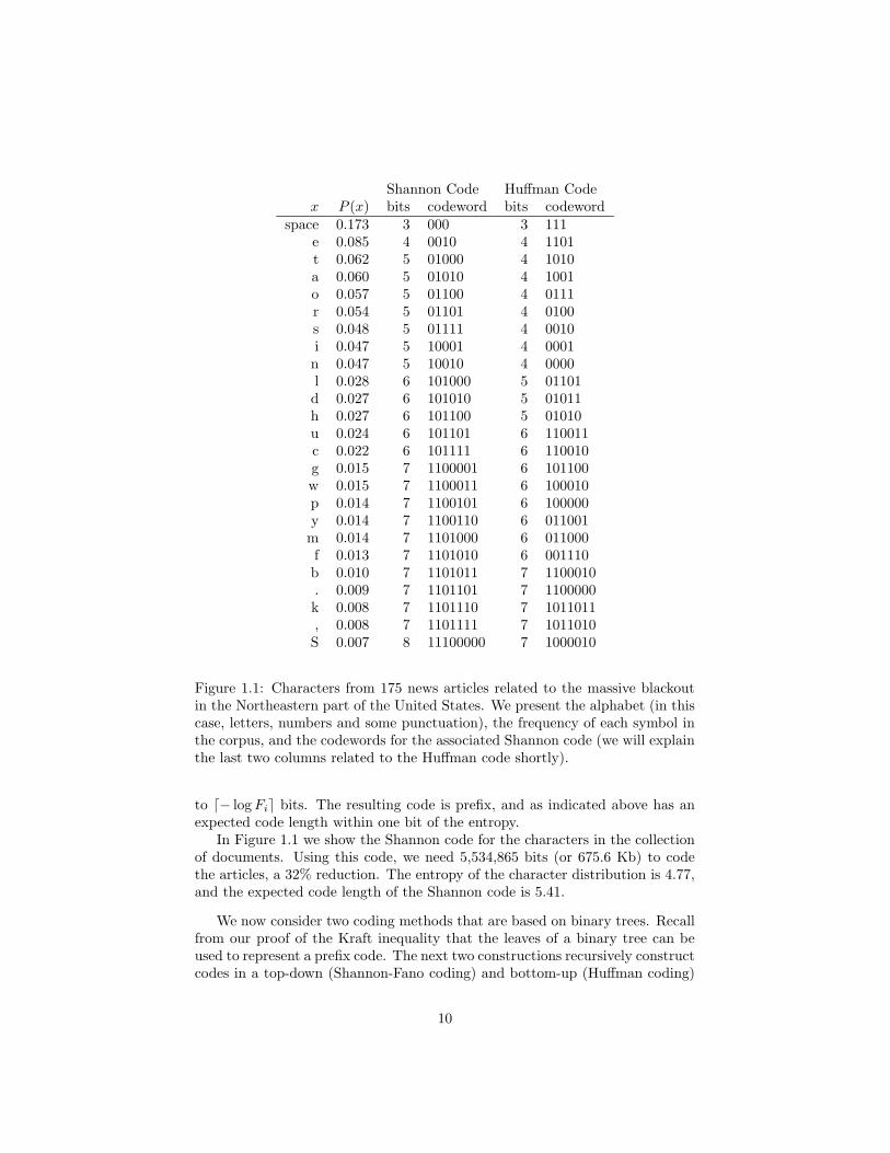
Figure 1.1: Characters from 175 news articles related to the massive blackoutin the Northeastern part of the United States. We present the alphabet (in thiscase, letters, numbers and some punctuation), the frequency of each symbol inthe corpus, and the codewords for the associated Shannon code (we will explainthe last two columns related to the Huffman code shortly).

to d− logFie bits. The resulting code is prefix, and as indicated above has anexpected code length within one bit of the entropy.

In Figure 1.1 we show the Shannon code for the characters in the collectionof documents. Using this code, we need 5,534,865 bits (or 675.6 Kb) to codethe articles, a 32% reduction. The entropy of the character distribution is 4.77,and the expected code length of the Shannon code is 5.41.

We now consider two coding methods that are based on binary trees. Recallfrom our proof of the Kraft inequality that the leaves of a binary tree can beused to represent a prefix code. The next two constructions recursively constructcodes in a top-down (Shannon-Fano coding) and bottom-up (Huffman coding)

10

fashion.

Example 1.6 (Shannon-Fano). This is a top-down method for forming abinary tree that will characterize a prefix code.

1. List all the possible messages, with their probabilities, in decreasing prob-ability order

2. Divide the list into two parts of (roughly) equal probability

3. Start the code for those messages in the first part with a 0 bit and forthose in the second part with a 1

4. Continue recursively until each subdivision contains just one message

It is possible to show that for the Shannon-Fano code,

H(P ) ≤ L ≤ H(P ) + 2. (1.9)

To illustrate the process, consider a six-symbol alphabet X = {a, e, i, o, u, !}.We give the probability function in Figure 1.6; note that we have sorted thesymbols in terms of their frequency. The entropy of this distribution is 2.45.Note that the expected code length of the resulting Shannon-Fano code is 2.5bits. In Figure 1.6, we compare this code length to that of the Shannon codebuilt from the same frequency table. Here, the Shannon code has an expectedcode length of 3 bits.

Shannon-Fano code (or any prefix code) can be re-expressed in terms of thegame of 20 questions. Suppose we want to find a sequence of yes-no questions todetermine an object from a class of objects with a known probability distribu-tion. We first group the objects into two subsets of (roughly) equal probabilitiesand ask which subset contains the object, and so on. This is exactly how theShnnon-Fano code was constructed. For any prefix code, there is a binary treewith leaf nodes as the code words for the objects. We start from the root of thetree, and group the objects into two subsets according to whether the objectsare the descendants of the left branch or the right branch and ask the questionwhether the object is in the left subset or the right subset, and so on. In termsof the expected number of questions asked, the optimal sequence of questionscorresponds to the Huffman code which we will now begin to introduce.

In his 1948 masterpiece, Shannon solved the source coding problem when themessage gets longer and longer (the entropy rate is achieved in the limit) and thisis the celebrated Shannon’s source coding theorem which we will take up later.However, he left open the optimal coding question for a fixed size alphabet.That is, among all prefix codes, which code gives the shortest expected codelength with respect to a message generating distribution P . Even though weknow the Shannon code gets close to the lower bound entropy within one bit, inthe finite case, the entropy might not be achievable. Huffman (1952) solved thisfinite sample optimality problem by showing that the Huffman code obtains theshortest average code length among all prefix codes. This is a surprising result

11

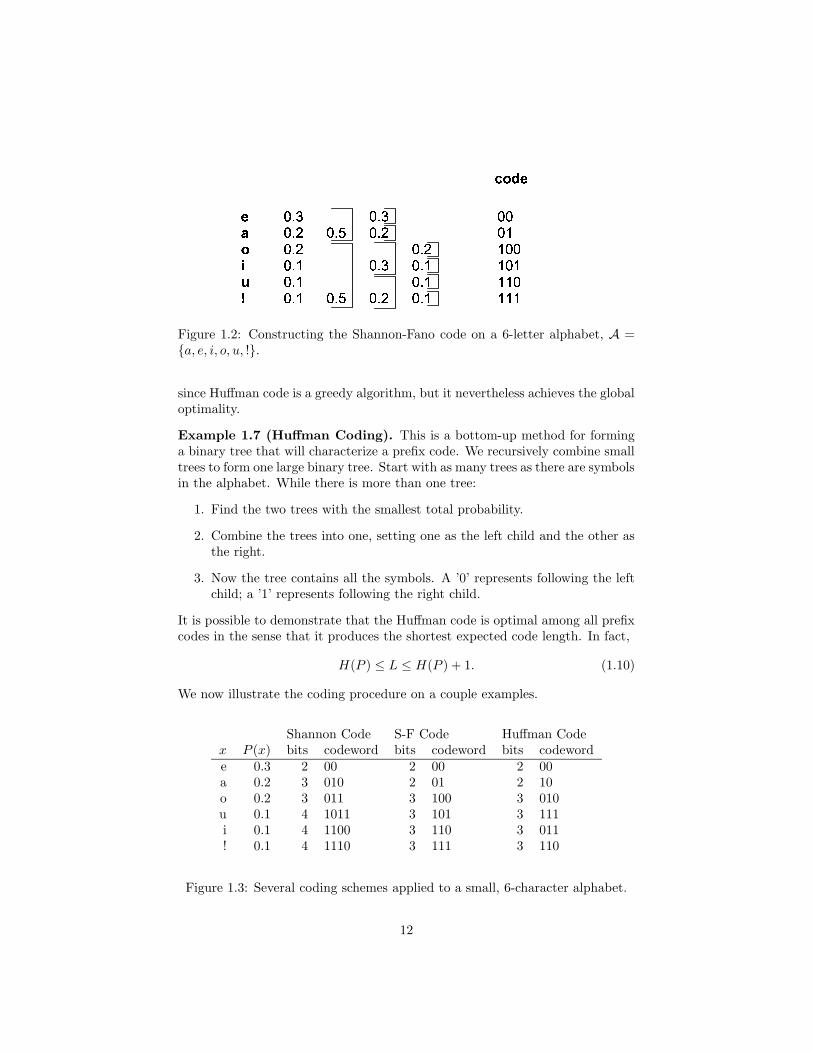
Figure 1.2: Constructing the Shannon-Fano code on a 6-letter alphabet, A ={a, e, i, o, u, !}.

since Huffman code is a greedy algorithm, but it nevertheless achieves the globaloptimality.

Example 1.7 (Huffman Coding). This is a bottom-up method for forminga binary tree that will characterize a prefix code. We recursively combine smalltrees to form one large binary tree. Start with as many trees as there are symbolsin the alphabet. While there is more than one tree:

1. Find the two trees with the smallest total probability.

2. Combine the trees into one, setting one as the left child and the other asthe right.

3. Now the tree contains all the symbols. A ’0’ represents following the leftchild; a ’1’ represents following the right child.

It is possible to demonstrate that the Huffman code is optimal among all prefixcodes in the sense that it produces the shortest expected code length. In fact,

H(P ) ≤ L ≤ H(P ) + 1. (1.10)

We now illustrate the coding procedure on a couple examples.

Shannon Code S-F Code Huffman Codex P (x) bits codeword bits codeword bits codeworde 0.3 2 00 2 00 2 00a 0.2 3 010 2 01 2 10o 0.2 3 011 3 100 3 010u 0.1 4 1011 3 101 3 111i 0.1 4 1100 3 110 3 011! 0.1 4 1110 3 111 3 110

Figure 1.3: Several coding schemes applied to a small, 6-character alphabet.

12

(11)

a(0)

(10)cb

C : X → {0, 1}∗ = strings of 0’s and 1’s

a → 0

b → 10

c → 11

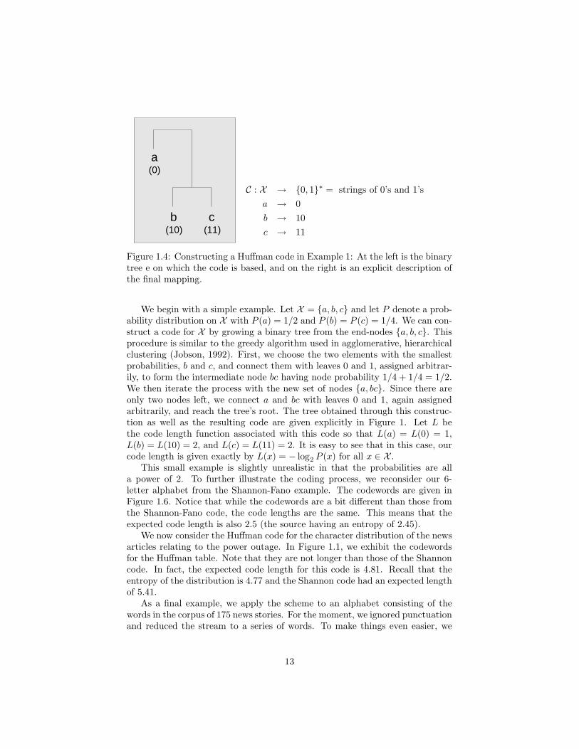
Figure 1.4: Constructing a Huffman code in Example 1: At the left is the binarytree e on which the code is based, and on the right is an explicit description ofthe final mapping.

We begin with a simple example. Let X = {a, b, c} and let P denote a prob-ability distribution on X with P (a) = 1/2 and P (b) = P (c) = 1/4. We can con-struct a code for X by growing a binary tree from the end-nodes {a, b, c}. Thisprocedure is similar to the greedy algorithm used in agglomerative, hierarchicalclustering (Jobson, 1992). First, we choose the two elements with the smallestprobabilities, b and c, and connect them with leaves 0 and 1, assigned arbitrar-ily, to form the intermediate node bc having node probability 1/4 + 1/4 = 1/2.We then iterate the process with the new set of nodes {a, bc}. Since there areonly two nodes left, we connect a and bc with leaves 0 and 1, again assignedarbitrarily, and reach the tree’s root. The tree obtained through this construc-tion as well as the resulting code are given explicitly in Figure 1. Let L bethe code length function associated with this code so that L(a) = L(0) = 1,L(b) = L(10) = 2, and L(c) = L(11) = 2. It is easy to see that in this case, ourcode length is given exactly by L(x) = − log2 P (x) for all x ∈ X .

This small example is slightly unrealistic in that the probabilities are alla power of 2. To further illustrate the coding process, we reconsider our 6-letter alphabet from the Shannon-Fano example. The codewords are given inFigure 1.6. Notice that while the codewords are a bit different than those fromthe Shannon-Fano code, the code lengths are the same. This means that theexpected code length is also 2.5 (the source having an entropy of 2.45).

We now consider the Huffman code for the character distribution of the newsarticles relating to the power outage. In Figure 1.1, we exhibit the codewordsfor the Huffman table. Note that they are not longer than those of the Shannoncode. In fact, the expected code length for this code is 4.81. Recall that theentropy of the distribution is 4.77 and the Shannon code had an expected lengthof 5.41.

As a final example, we apply the scheme to an alphabet consisting of thewords in the corpus of 175 news stories. For the moment, we ignored punctuationand reduced the stream to a series of words. To make things even easier, we

13

0 2 4 6 8

0

2

4

6

8

log of order

log

coun

t

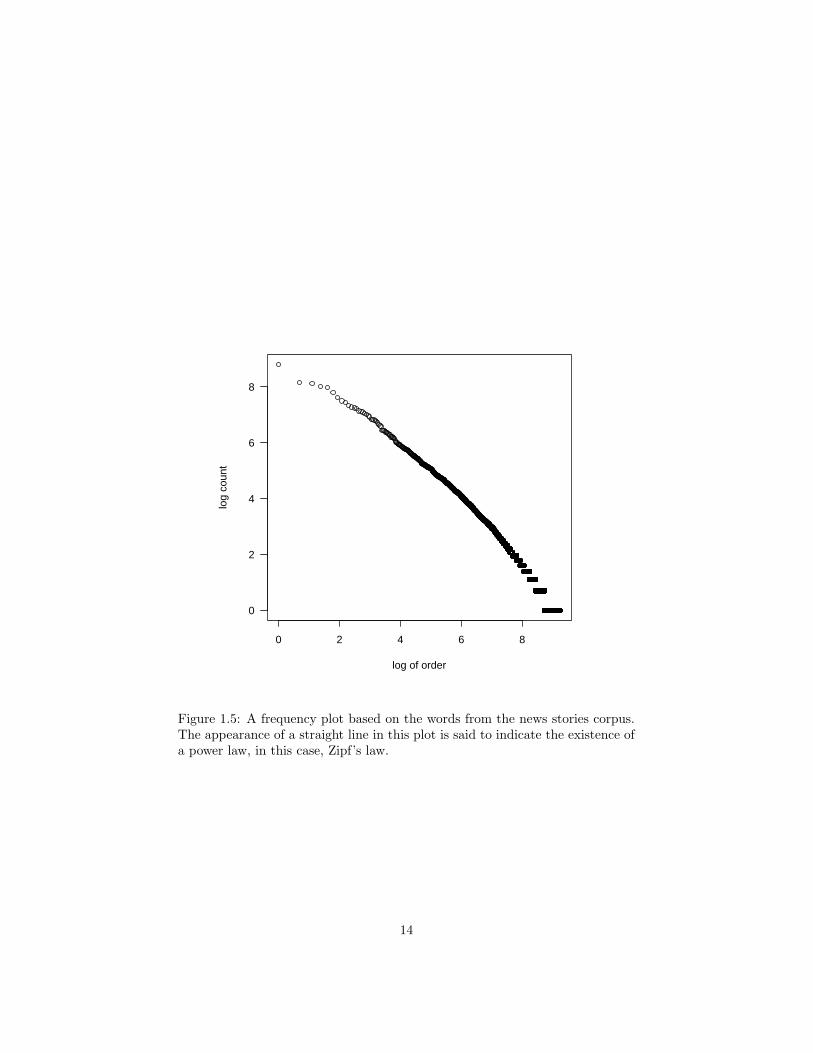
Figure 1.5: A frequency plot based on the words from the news stories corpus.The appearance of a straight line in this plot is said to indicate the existence ofa power law, in this case, Zipf’s law.

14

regularized the words in the sense that we removed all the capitalization. Inall, there are 10,269 words. The distribution of counts is quite skewed, andseems to obey Zipf’s law; see Figure 1.7. From this large alphabet, we thenbuild both the Shannon code and the Huffman code. In Figure 1.7 we presentboth a sample of the frequency distribution as well as the codewords. Again, theHuffman table tends to have shorter codewords. The entropy of the distributionis 10.02, and the expected code lengths are 10.43 for Shannon and 10.05 forHuffman. In terms of actual compression, this means that we can encode thewords with 1,665,567 bits (208,196 bytes or 203Kb) for Shannon and 1,605,460bits (200,683 bits or 196Kb) for Huffman. This represents a tremendous savingsover the character-based codes we’ve considered so far. Naturally, by reducingthe data to lower-case words, we have simplified the stream and have made thejob easier. Still, if we were to have coded a file consisting of the stream of words(inserting a space between each) in ASCII, it would require 945,513 bytes or923Kb.

A modification of Shannon code removes the sorting step by encoding themiddle points in the jumps of the CDF and this gives the Shannon-Fano-Eliascode which is particularly convenient for block coding.

Example 1.8 (Shannon-Fano-Elias). Let X = {1, 2, . . . ,m} and Q(x) > 0for x ∈ X . Define the cumulative distribution function F (x) and the so-calledmodified distribution function F (x) to be

F (x) =∑

a≤x

Q(a) and F (x) =∑

a<x

+1

2Q(x) (1.11)

Since Q(x) is positive on X , the cumulative distribution function has the prop-erty that F (a) 6= F (a′) if a 6= a′. Looking at F , it is clear that we can mapF (x) back to x and hence F (x) can be used to encode x. In general, as a set ofcodewords, F (x) can be quite complicated, and might even require an infinitenumber of bits to describe. Instead, we build a code from a truncated expansionof F (x). We round to l(x) bits, meaning

F (x) − bF (x)cl(x) <1

2l(x)(1.12)

Now, if we set l(x) = d− logQ(x)e + 1, then

1

2l(x)<Q(x)

2= F (x) − F (x− 1) (1.13)

so that the truncated value bF (x)cl(x) can be mapped back to x using thecumulative distribution function. Like Huffman’s algorithm, this constructionalso produces a prefix code (using F (x) would not guarantee this). Also, thiscode also uses shorter code words for less frequently observed symbols.

In Figure 1.7 we exhibit the codewords for this construction. The maindifference between this code and the Shannon code is that the symbols are notsorted according to their probability before code construction, so that some

15

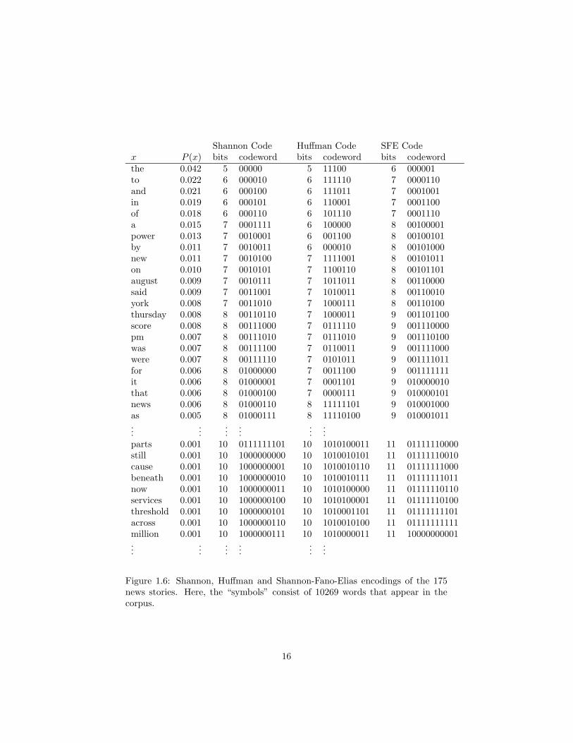
Shannon Code Huffman Code SFE Codex P (x) bits codeword bits codeword bits codewordthe 0.042 5 00000 5 11100 6 000001to 0.022 6 000010 6 111110 7 0000110and 0.021 6 000100 6 111011 7 0001001in 0.019 6 000101 6 110001 7 0001100of 0.018 6 000110 6 101110 7 0001110a 0.015 7 0001111 6 100000 8 00100001power 0.013 7 0010001 6 001100 8 00100101by 0.011 7 0010011 6 000010 8 00101000new 0.011 7 0010100 7 1111001 8 00101011on 0.010 7 0010101 7 1100110 8 00101101august 0.009 7 0010111 7 1011011 8 00110000said 0.009 7 0011001 7 1010011 8 00110010york 0.008 7 0011010 7 1000111 8 00110100thursday 0.008 8 00110110 7 1000011 9 001101100score 0.008 8 00111000 7 0111110 9 001110000pm 0.007 8 00111010 7 0111010 9 001110100was 0.007 8 00111100 7 0110011 9 001111000were 0.007 8 00111110 7 0101011 9 001111011for 0.006 8 01000000 7 0011100 9 001111111it 0.006 8 01000001 7 0001101 9 010000010that 0.006 8 01000100 7 0000111 9 010000101news 0.006 8 01000110 8 11111101 9 010001000as 0.005 8 01000111 8 11110100 9 010001011...

......

......

...parts 0.001 10 0111111101 10 1010100011 11 01111110000still 0.001 10 1000000000 10 1010010101 11 01111110010cause 0.001 10 1000000001 10 1010010110 11 01111111000beneath 0.001 10 1000000010 10 1010010111 11 01111111011now 0.001 10 1000000011 10 1010100000 11 01111110110services 0.001 10 1000000100 10 1010100001 11 01111110100threshold 0.001 10 1000000101 10 1010001101 11 01111111101across 0.001 10 1000000110 10 1010010100 11 01111111111million 0.001 10 1000000111 10 1010000011 11 10000000001...

......

......

...

Figure 1.6: Shannon, Huffman and Shannon-Fano-Elias encodings of the 175news stories. Here, the “symbols” consist of 10269 words that appear in thecorpus.

16

extra effort has to be expended to guarantee the prefix property of the resultingcode.

So far, we have discussed four coding schemes, Shannon, Shannon-Fano,Huffman, and Shannon-Fano-Elias. We have seen that in some cases, we areclose to the entropy bound, in others not so close. In the case of Huffmancode, it is common to consider an alphabet formed by blocks of length n fromthe source. If the blocks are too small and the alphabet is small, then codingcannot provide much gains. For example, if we try to encode a string of 0’s and1’s, taking blocks of size 1 will not produce any compression gains. No matterhow we code, we will always be forced to communicate one bit for each inputbit. This holds for every prefix code and when H(P ) is small, this is far awayfrom the entropy lower bound given by the Gibbs’ inequality.

In general, we can improve the behavior of these schemes by encoding largerblocks of data. That is, rather than work with a single symbol at a time, weconsider strings of length n. To see why there might be an advantage to doingthis, let Pn(x1, . . . , xn) = P (x1) · · ·P (xn). Then,

H(Pn) ≤ ELn ≤ H(Pn) + 1 (1.14)

Since we have an iid sequence of symbols, the entropy can be written

H(Pn) =∑

H(P ) = nH(P ) (1.15)

so that per symbol we have

H(P ) ≤ L < H(P ) +1

n(1.16)

This means we can get arbitrarily close to the entropy limit by considering longerand longer blocks. This is the celebrated Shannon’s source coding theorem. Nowlet us prepare ourselves for its proof by studying the entropy function a bit indepth.

1.2.4 Entropy

Given a probability function P defined on a discrete alphabet X , we define theentropy H(P ) to be

H(P ) = −∑

x∈X

P (x) logP (x) . (1.17)

The logarithm in this expression is usually in base 2, and the units of entropyare referred to as bits.

• H(P ) ≥ 0

• Hb(P ) = logb aHa(P )

• H(X|Y ) ≤ H(X) with equality only if X and Y are independent

17

0.0 0.2 0.4 0.6 0.8 1.0

0.0

0.1

0.2

0.3

0.4

0.5

0.6

0.7

p

entr

opy

p1

p2

0.0 0.2 0.4 0.6 0.8 1.0

0.0

0.2

0.4

0.6

0.8

1.0

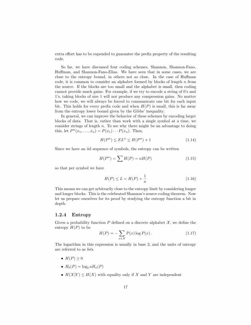
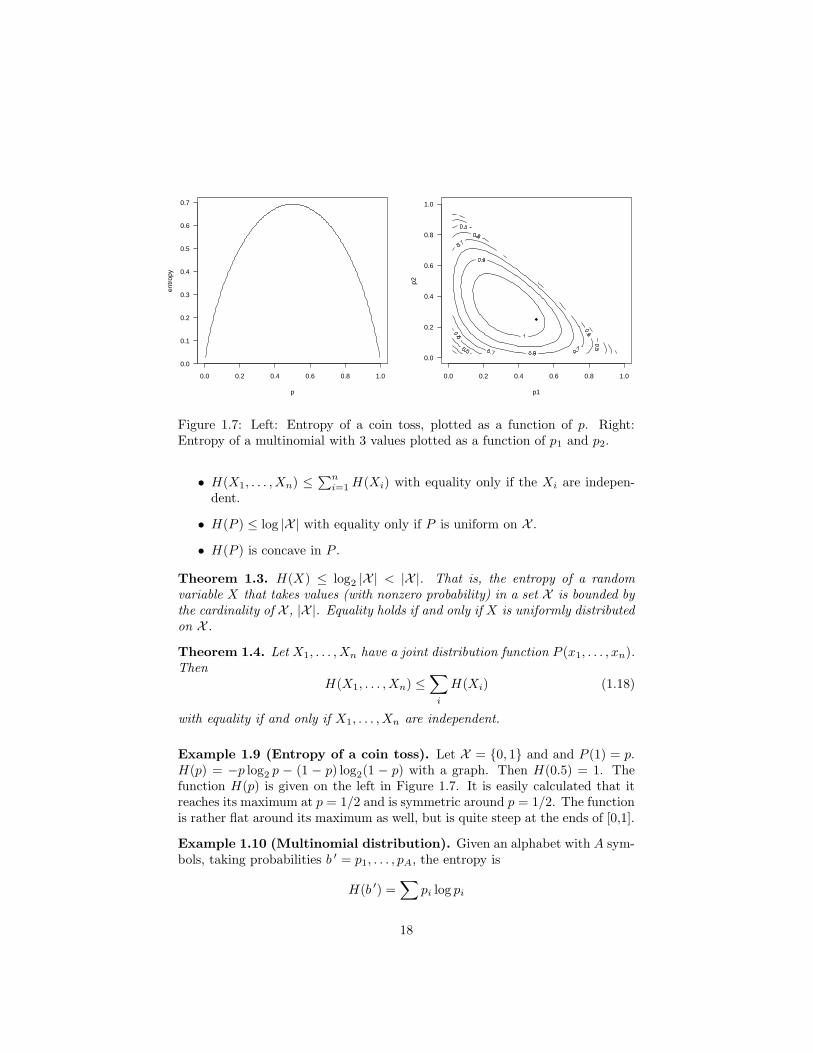
Figure 1.7: Left: Entropy of a coin toss, plotted as a function of p. Right:Entropy of a multinomial with 3 values plotted as a function of p1 and p2.

• H(X1, . . . , Xn) ≤ ∑ni=1H(Xi) with equality only if the Xi are indepen-

dent.

• H(P ) ≤ log |X | with equality only if P is uniform on X .

• H(P ) is concave in P .

Theorem 1.3. H(X) ≤ log2 |X | < |X |. That is, the entropy of a randomvariable X that takes values (with nonzero probability) in a set X is bounded bythe cardinality of X , |X |. Equality holds if and only if X is uniformly distributedon X .

Theorem 1.4. Let X1, . . . , Xn have a joint distribution function P (x1, . . . , xn).Then

H(X1, . . . , Xn) ≤∑

i

H(Xi) (1.18)

with equality if and only if X1, . . . , Xn are independent.

Example 1.9 (Entropy of a coin toss). Let X = {0, 1} and and P (1) = p.H(p) = −p log2 p − (1 − p) log2(1 − p) with a graph. Then H(0.5) = 1. Thefunction H(p) is given on the left in Figure 1.7. It is easily calculated that itreaches its maximum at p = 1/2 and is symmetric around p = 1/2. The functionis rather flat around its maximum as well, but is quite steep at the ends of [0,1].

Example 1.10 (Multinomial distribution). Given an alphabet with A sym-bols, taking probabilities b ′ = p1, . . . , pA, the entropy is

H(b ′) =∑

pi log pi

18

For 3 values, b ′ = (p1, p2, p3). The function H(b ′) is given on the right inFigure 1.7, plotted as a function of p1 and p2. The point marked in this figure(0.5,0.25) indicates the entropy value for our toy example given above, wherethe the alphabet X = {a, b, c}.

1.2.5 Axiomatic definition of entropy

Below we list a number of properties that seem reasonable for a measure ofinformation. Various authors have shown that collections of these propertiesare in fact sufficient to prove that entropy must take the form defined above.

Continuity H2(p, 1 − p) is a continuous function of p. This makes sense be-cause we would not want small changes in p to yield large differences ininformation.

Normalization H2(0.5, 0.5) = 1. Simply, this states that choosing betweentwo equally likely alternatives should require a single bit of information.

Monotonicity For pj = 1/m, the entropy H(1/m, . . . , 1/m) should be an in-creasing function of m. When dealing with choices between equally likelyevents, there is more choice or uncertainty when there are more possibleevents.

Symmetry The functionH(p1, . . . , pm) is a symmetric in its arguments p1, . . . , pm.

Conditioning Hm(p1, . . . , pm) = Hm−1(p1+p2, p2, . . . , pm)+(p1+p2)H2( p1

p1+p2, p2

p1+p2)

Theorem 1.5. If a function satisfies continuity, normalizaion and the condi-tioning princple, then

Hm(p1, . . . , pm) = −m

∑

i=1

pi log pi for m = 2, 3, . . .

1.2.6 Shannon’s source coding theorem

Even though Shannon’s source coding theorem holds for ergodic sequences, wecover only the iid case in this section. A sequence of iid symbols X1, ..., Xn

from X , each with entropy H(P ), can be compressed into more than nH(P )bits with negligible loss of information as n → ∞; conversely, Gibbs inequalityensures the entropy nH(P ) for the product measure as a lower bound.

Theorem 1.6 (Asymptotic Equipartition Property (AEP)). If X1, ..., Xn

are iid with a distribution P ,

− 1

nlog2 P (X1, ..., Xn) → H(P ) (1.19)

in probability as n tends to infinity.

Proof. The result follows from the weak law of large numbers.

19

Corollary 1.1. Under the assumptions of the above theorem, the average codelengths per symbol of the Shannon and Fano-Shannon-Elias codes on X n tendto the entropy H(P ) as the sequence gets longer and longer.

One can interpret or re-write the above result using the terminology of atypical set.

Definition 1 (Typical Set). For a given ε > 0, the typical set is defined

A(n)ε = {xn ∈ X : 2−n(H(P )+ε) ≤ P (xn) ≤ 2−n(H(P )−ε)} ∈ Xn.

The set A(n)ε is typical in the sense that the strings xn ∈ A

(n)ε account

for most of the probability in the product space, X n, and the probability of

each string xn ∈ A(n)ε is close to uniform; that is, the cardiality of A

(n)ε is

approximately 2nH(P ), and the probability of each string xn ∈ A(n)ε is about

2−nH(P ). When P is the uniform distribution on X , we have seen that the

entropy is log |X |. For the typical set, we have log2A(n)ε ≈ log2 2nH(P ) = nH(P ).

Hence, through the notion of a typical set, the uniform distribution emerges asan important tool for understanding the entropy of general P . These statementsare made precise by the following theorem:

Theorem 1.7. Given a probabiity distribution P on a set X , and iid obser-vations X1, . . . , Xn from P , we have the following results about the typical set

A(n)ε for ε > 0

1. If xn ∈ A(n)ε ,

∣

∣

∣

∣

− 1

nlog2 P (xn) −H(P )

∣

∣

∣

∣

< ε , (1.20)

2. For large n,

P(

A(n)ε

)

> 1 − ε , (1.21)

3. |A(n)ε | < 2n(H(P )+ε), and

4. For large n,∣

∣

∣A(n)

ε

∣

∣

∣> (1 − ε) 2n(H(P )−ε) (1.22)

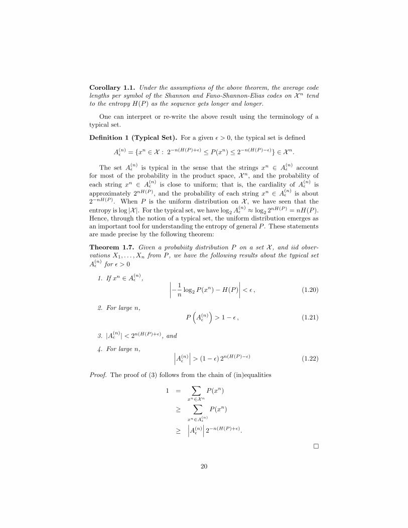
Proof. The proof of (3) follows from the chain of (in)equalities

1 =∑

xn∈Xn

P (xn)

≥∑

xn∈A(n)ε

P (xn)

≥∣

∣

∣A(n)

ε

∣

∣

∣2−n(H(P )+ε).

20

An entropy-achieving block coding scheme can be devised based on the corol-lary. For a given ε > 0, first we use one bit to indicate whether a sequence

xn ∈ Xn is in A(n)ε or not; we enumerate the sequences in A

(n)ε in lexicographic

order to give each sequence an integer index which is the code for this sequence.This takes less than n(H(P ) + ε) + 2 bits. For the sequences in the compliment

of A(n)ε , it takes at most n log2 |X | + 2 bits to encode. As a result, this coding

scheme has average code length per symbol approximates the entropy rate on

A(n)ε .

All the codes introduced earlier when applied to the block alphabet X n leadto the entropy rate in the limit. But some are easier to implement on the blockthan others. In particular, Huffman and Shannon codes need sorting which isa demanding computational task for a large alphabet X n when n is not small.It is particularly hard to move from one block size to the next for these codes.The Shannon-Fano-Elias code, however, is easily updated when the block sizechanges and has acquired a new name, Arithmetic Code, when applied to blocks.

Example 1.11 (Arithmetic Code). We end this set of examples with anencoding scheme that builds on the Shannon code and the Shannon-Fano-Eliascode. Assume we have a model Q that we want to use to compress strings froma particular source. The distribution Q does not have to correspond to the truedata-generating distribution. Suppose we have a string x1, x2, . . . , xn that wewant to compress. In the simplest case, our model Q might assume that eachsymbol appears in the string independently. We might also consider a Markovmodel in which Q(xi) = Q(xi|xi−1). No matter how we specify the model,it is important that we can compute the probability of xi given the previouselements of the sequence.

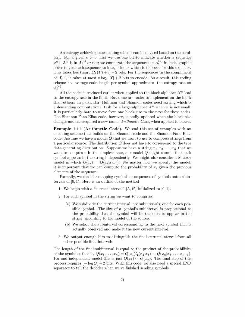
Formally, we consider mapping symbols or sequences of symbols onto subin-tervals of [0, 1). Here is an outline of the method

1. We begin with a “current interval” [L,H) initialized to [0, 1).

2. For each symbol in the string we want to compress

(a) We subdivide the current interval into subintervals, one for each pos-sible symbol. The size of a symbol’s subinterval is proportional tothe probability that the symbol will be the next to appear in thestring, according to the model of the source.

(b) We select the subinterval corresponding to the next symbol that isactually observed and make it the new current interval.

3. We output enough bits to distinguish the final current interval from allother possible final intervals.

The length of the final subinterval is equal to the product of the probabilitiesof the symbols; that is, Q(x1, . . . , xn) = Q(x1)Q(x2|x1) · · ·Q(xn|x1, . . . , xn−1).For and independent model this is just Q(x1) · · ·Q(xn). The final step of thisprocess requires b− logQc+ 2 bits. With this code, we also need a special ENDseparator to tell the decoder when we’ve finished sending symbols.

21

Next symbol L H0.0 1.0

a 0.0 0.9a 0.0 0.81a 0.0 0.729a 0.0 0.6561a 0.0 0.59049a 0.0 0.531441a 0.0 0.4782969

END 0.43046721 0.4782969

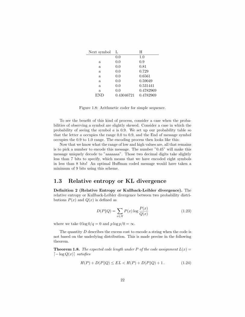
Figure 1.8: Arithmetic coder for simple sequence.

To see the benefit of this kind of process, consider a case when the proba-bilities of observing a symbol are slightly skewed. Consider a case in which theprobability of seeing the symbol a is 0.9. We set up our probability table sothat the letter a occupies the range 0.0 to 0.9, and the End of message symboloccupies the 0.9 to 1.0 range. The encoding process then looks like this:

Now that we know what the range of low and high values are, all that remainsis to pick a number to encode this message. The number ”0.45” will make thismessage uniquely decode to ”aaaaaaa”. Those two decimal digits take slightlyless than 7 bits to specify, which means that we have encoded eight symbolsin less than 8 bits! An optimal Huffman coded message would have taken aminimum of 9 bits using this scheme.

1.3 Relative entropy or KL divergence

Definition 2 (Relative Entropy or Kullback-Leibler divergence). Therelative entropy or Kullback-Leibler divergence between two probability distri-butions P (x) and Q(x) is defined as

D(P‖Q) =∑

x∈X

P (x) logP (x)

Q(x)(1.23)

where we take 0 log 0/q = 0 and p log p/0 = ∞.

The quantity D describes the excess cost to encode a string when the code isnot based on the underlying distribution. This is made precise in the followingtheorem.

Theorem 1.8. The expected code length under P of the code assignment L(x) =d− logQ(x)e satisfies

H(P ) +D(P‖Q) ≤ EL < H(P ) +D(P‖Q) + 1 . (1.24)

22

For an iid sequence of size n, if the code is based on a product measure Qn,the average expected excess code length for average expected redundancy

|ELn/n−H(P )| ≤ D(P‖Q) + 1/n. (1.25)

Relative entropy or KL divergence is easily extendible to the continuouscase by replacing summation with an integral operator. (If we try to apply thesummation definition to a continuous distribution, we end up with a value ofinfinity.) But one may argue that for a fixed precision, the essential informationabout the distribution is captured by the so-called differential entropy.

Definition 3 (Differential Entropy). Given a continuous distribution witha positive density function f on Rd, its differential entropy is defined as

H(f) = −∫

Rd

f(x) log2 f(x)dx, (1.26)

with the convention that 0 log2 0 = 0.

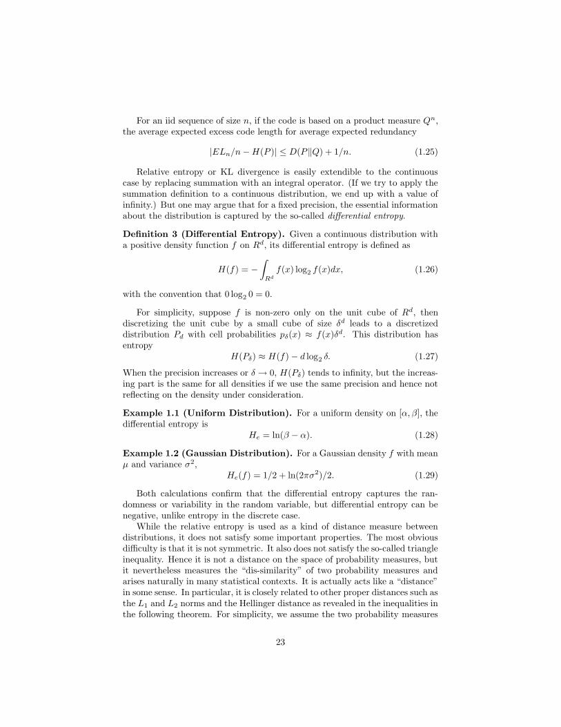
For simplicity, suppose f is non-zero only on the unit cube of Rd, thendiscretizing the unit cube by a small cube of size δd leads to a discretizeddistribution Pd with cell probabilities pδ(x) ≈ f(x)δd. This distribution hasentropy

H(Pδ) ≈ H(f) − d log2 δ. (1.27)

When the precision increases or δ → 0, H(Pδ) tends to infinity, but the increas-ing part is the same for all densities if we use the same precision and hence notreflecting on the density under consideration.

Example 1.1 (Uniform Distribution). For a uniform density on [α, β], thedifferential entropy is

He = ln(β − α). (1.28)

Example 1.2 (Gaussian Distribution). For a Gaussian density f with meanµ and variance σ2,

He(f) = 1/2 + ln(2πσ2)/2. (1.29)

Both calculations confirm that the differential entropy captures the ran-domness or variability in the random variable, but differential entropy can benegative, unlike entropy in the discrete case.

While the relative entropy is used as a kind of distance measure betweendistributions, it does not satisfy some important properties. The most obviousdifficulty is that it is not symmetric. It also does not satisfy the so-called triangleinequality. Hence it is not a distance on the space of probability measures, butit nevertheless measures the “dis-similarity” of two probability measures andarises naturally in many statistical contexts. It is actually acts like a “distance”in some sense. In particular, it is closely related to other proper distances such asthe L1 and L2 norms and the Hellinger distance as revealed in the inequalities inthe following theorem. For simplicity, we assume the two probability measures

23

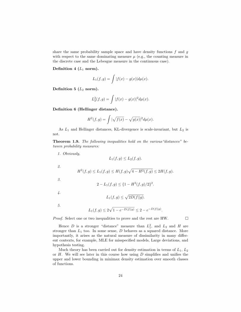
share the same probability sample space and have density functions f and gwith respect to the same dominating measure µ (e.g., the counting measure inthe discrete case and the Lebesgue measure in the continuous case).

Definition 4 (L1 norm).

L1(f, g) =

∫

|f(x) − g(x)|dµ(x).

Definition 5 (L2 norm).

L22(f, g) =

∫

|f(x) − g(x)|2dµ(x).

Definition 6 (Hellinger distance).

H2(f, g) =

∫

|√

f(x) −√

g(x)|2dµ(x).

As L1 and Hellinger distances, KL-divergence is scale-invariant, but L2 isnot.

Theorem 1.9. The following inequalities hold on the various“distances” be-tween probability measures:

1. Obviously,L1(f, g) ≤ L2(f, g).

2.H2(f, g) ≤ L1(f, g) ≤ H(f, g)

√

4 −H2(f, g) ≤ 2H(f, g).

3.2 − L1(f, g) ≤ {1 −H2(f, g)/2}2.

4.L1(f, g) ≤

√

2D(f ||g).

5.L1(f, g) ≤ 2

√

1 − e−D(f ||g) ≤ 2 − e−D(f ||g).

Proof. Select one or two inequalities to prove and the rest are HW.

Hence D is a stronger “distance” measure than L21, and L2 and H are

stronger than L1 too. In some sense, D behaves as a squared distance. Moreimportantly, it arises as the natural measure of dissimilarity in many differ-ent contexts, for example, MLE for misspecified models, Large deviations, andhypothesis testing.

Much theory has been carried out for density estimation in terms of L1, L2

or H. We will see later in this course how using D simplifies and unifies theupper and lower bounding in minimax density estimation over smooth classesof functions.

24

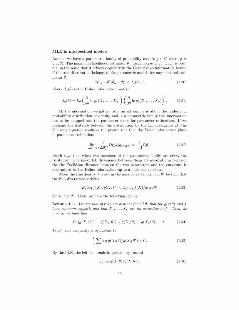
MLE in misspecified models

Assume we have a parametric family of probability models g ∈ G where g =g(x; θ). The maximum likelihood estimator θ = arg maxθ gθ(x1, . . . , xn) is opti-mal in the sense that it achieves equality in the Cramer-Rao information boundif the true distribution belongs to the parametric model: for any unbiased esti-mator θn

E(θn − θ)(θn − θ)′ ≥ Jn(θ)−1, (1.30)

where Jn(θ) is the Fisher information matrix,

Jn(θ) = Eθ

(

∂

∂θln gθ(X1, . . . , Xn)

) (

∂

∂θln gθ(X1, . . . , Xn)

)′

. (1.31)

All the information we gather from an iid sample is about the underlyingprobability distribution or density and in a parametric family this informationhas to be mapped into the parameter space for parameter estimation. If wemeasure the distance between the distribution by the KL divergence D, thefollowing equation confirms the pivotal role that the Fisher information playsin parameter estimation:

lim∆θ→0

1

(∆θ)2D(gθ‖gθ+∆θ) =

1

ln 4I(θ), (1.32)

which says that when two members of the parametric family are close, the“distance” in terms of KL divergence between them are quadratic in terms ofthe the Euclidean distance between the two parameters and the curvature isdetermined by the Fisher information up to a universal constant.

When the true density f is not in the parametric family. Let θ∗ be such thatthe K-L divergence satisfies

Ef log f(X)/g(X; θ∗) < Ef log f(X)/g(X; θ) (1.33)

for all θ 6= θ∗. Then, we have the following lemma.

Lemma 1.1. Assume that g(x; θ) are distinct for all θ; that the g(x; θ) and fhave common support; and that X1, . . . , Xn are iid according to f . Then, asn→ ∞ we have that

Pf (g(X1; θ∗) · · · g(Xn; θ∗) > g(X1; θ) · · · g(Xn; θ)) → 1 . (1.34)

Proof. The inequality is equivalent to

1

n

∑

i

log g(Xi; θ)/g(Xi; θ∗) < 0 . (1.35)

By the LLN, the left side tends in probability toward

Ef log g(X; θ)/g(X; θ∗) . (1.36)

25

But, rewriting

Ef log g(X; θ)/g(X; θ∗) = Ef log g(X; θ) − Ef log g(X; θ∗) (1.37)

= −Ef log f(X)/g(X; θ) + Ef log f(X)/g(X; θ∗)(1.38)

< 0 . (1.39)

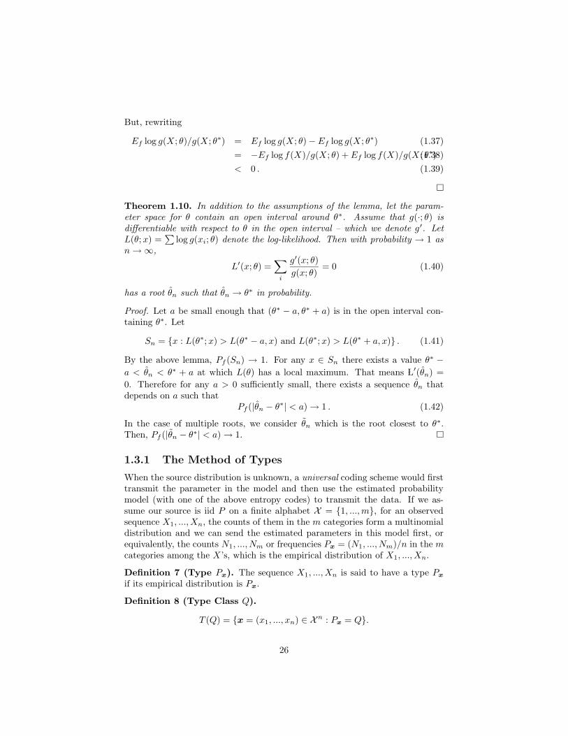
Theorem 1.10. In addition to the assumptions of the lemma, let the param-eter space for θ contain an open interval around θ∗. Assume that g(·; θ) isdifferentiable with respect to θ in the open interval – which we denote g ′. LetL(θ;x) =

∑

log g(xi; θ) denote the log-likelihood. Then with probability → 1 asn→ ∞,

L′(x; θ) =∑

i

g′(x; θ)

g(x; θ)= 0 (1.40)

has a root θn such that θn → θ∗ in probability.

Proof. Let a be small enough that (θ∗ − a, θ∗ + a) is in the open interval con-taining θ∗. Let

Sn = {x : L(θ∗;x) > L(θ∗ − a, x) and L(θ∗;x) > L(θ∗ + a, x)} . (1.41)

By the above lemma, Pf (Sn) → 1. For any x ∈ Sn there exists a value θ∗ −a < θn < θ∗ + a at which L(θ) has a local maximum. That means L′(θn) =

0. Therefore for any a > 0 sufficiently small, there exists a sequence θn thatdepends on a such that

Pf (|θn − θ∗| < a) → 1 . (1.42)

In the case of multiple roots, we consider θn which is the root closest to θ∗.Then, Pf (|θn − θ∗| < a) → 1.

1.3.1 The Method of Types

When the source distribution is unknown, a universal coding scheme would firsttransmit the parameter in the model and then use the estimated probabilitymodel (with one of the above entropy codes) to transmit the data. If we as-sume our source is iid P on a finite alphabet X = {1, ...,m}, for an observedsequence X1, ..., Xn, the counts of them in the m categories form a multinomialdistribution and we can send the estimated parameters in this model first, orequivalently, the counts N1, ..., Nm or frequencies Px = (N1, ..., Nm)/n in the mcategories among the X’s, which is the empirical distribution of X1, ..., Xn.

Definition 7 (Type Px). The sequence X1, ..., Xn is said to have a type Px

if its empirical distribution is Px.

Definition 8 (Type Class Q).

T (Q) = {x = (x1, ..., xn) ∈ Xn : Px = Q}.

26

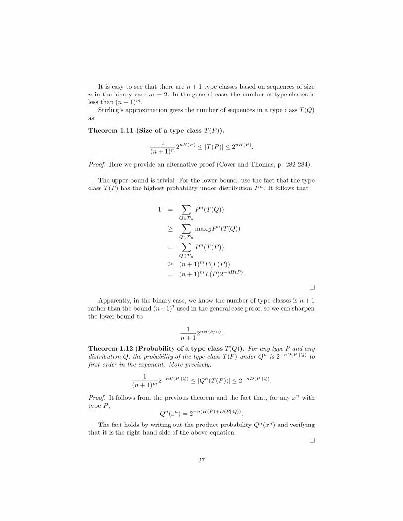
It is easy to see that there are n+ 1 type classes based on sequences of sizen in the binary case m = 2. In the general case, the number of type classes isless than (n+ 1)m.

Stirling’s approximation gives the number of sequences in a type class T (Q)as:

Theorem 1.11 (Size of a type class T (P )).

1

(n+ 1)m2nH(P ) ≤ |T (P )| ≤ 2nH(P ).

Proof. Here we provide an alternative proof (Cover and Thomas, p. 282-284):

The upper bound is trivial. For the lower bound, use the fact that the typeclass T (P ) has the highest probability under distribution P n. It follows that

1 =∑

Q∈Pn

Pn(T (Q))

≥∑

Q∈Pn

maxQPn(T (Q))

=∑

Q∈Pn

Pn(T (P ))

≥ (n+ 1)mP (T (P ))

= (n+ 1)mT (P )2−nH(P ).

Apparently, in the binary case, we know the number of type classes is n+ 1rather than the bound (n+1)2 used in the general case proof, so we can sharpenthe lower bound to

1

n+ 12nH(k/n).

Theorem 1.12 (Probability of a type class T (Q)). For any type P and anydistribution Q, the probability of the type class T (P ) under Qn is 2−nD(P ||Q) tofirst order in the exponent. More precisely,

1

(n+ 1)m2−nD(P ||Q) ≤ |Qn(T (P ))| ≤ 2−nD(P ||Q).

Proof. It follows from the previous theorem and the fact that, for any xn withtype P ,

Qn(xn) = 2−n(H(P )+D(P ||Q)).

The fact holds by writing out the product probability Qn(xn) and verifyingthat it is the right hand side of the above equation.

27

HW: prove LLN in terms of D using the above theorems. That is,D(Pxn ||P ) → 0 with probability 1.

Example 1.3 (Universal Source Coding). For a given sequence xn, it takesless than m log(n+ 1) bits to send over the type class information and if we usea uniform code over this type class (all the sequences have the same probabilityin a type class under an iid assumption on the source distribution), then it takeslog |T (Pxn)| ≤ nH(Pxn) bits to transmit the membership of the observed xn inthe type class. Hence the average code length of resulted two-part code L(xn)/ntends to H(P ) almost surely as n→ ∞ because H(Pxn) → H(P ) almost surely.

Read p. 279-291 of CT.

1.3.2 Large Deviations

Definition 9 (Exponent). A real number a is said to be the exponenet for asequence an, n ≥ 1, where an ≥ 0 and an → 0 if

limn→∞

(

− 1

nlog an

)

= −a .

Sanov’s Theorem

The Central Limit Theorem provides good approximations to events of “smalldeviations” from the typical, but fails to provide accurate estimates of “rareevents” or large deviations from the typical. These “rare event” calculationsarise in applications from hypothesis testing (which we will cover) to finance(estimating probability of large portfolio losses). The classical LD results canbe derived based on the method of types bounds we have just seen and we endwith a discussion of the general case. This rare probability often turns out to beexponential with a negative size factor (n in the iid case) and an exponent whichis describing how close the events to the typical in terms of the KL-divergence.

Theorem 1.13 (Sanov’s theorem). Let X1, ..., Xn be iid Q. Let E be a setof probability distributions on a finite alphabet X . Then

Qn(E) = Qn(E ∩ Pn) ≤ (n+ 1)m2−nD(P ∗||Q),

whereP ∗ = argminP∈ED(P ||Q),

is the distribution in E that is closest to P in KL divergence. If, in addition,the set E is the closure of its interior, then

1

nPn(E) → −D(P ∗||Q).

Proof. The upper bound is straightforward: the moral is that in the log scale andto the first order, the maximum probability in a summation of probabilities gives

28

the right answer. Here we need E to be nice so that we can find a distributionP ∈ E which is close to P ∗. Under the assumption on E, since ∪nPn is densein the set of all distributions on X n, we can find a sequence of distributions Pn

so that for n ≤ n0, Pn ∈ E ∩ Pn, and D(Pn||Q) → D(P ∗||Q). For n ≤ n0,

Qn(E) =∑

P∈E∩Pn

Qn(T (P ))

≥ Qn(T (Pn))

≥ 1

(n+ 1)m2−nD(Pn||Q),

which implies the lower bound.

In this characterization of a large deviations result, the set of probabilitiesE are used to describe the event of interest. We now give an example based onsample averages.

Example 1.4 (Sample averages). We now consider the probability of eventsbased on the sample mean, the simplest case being that the sample mean islarger than some threshold τ . Let X1, . . . , Xn be iid according to Q, with eachXi ∈ X = {0, . . . ,m}. To compute the probability

Pr(1

n

∑

i

Xi > τ)

We consider the set E

E = {P :

n∑

j=1

jP (j) > τ} (1.43)

We now want to minimize the KL divergence between elements in E and thedata generating distribution Q. Introducing Lagrange multipliers λ and ν wewant to minimize the following expression

∑

j

P (j) logP (j)

Q(j)− λ

∑

j

P (j)j + ν∑

j

P (j) .

The first multiplier λ is associated with the constraint on the sample mean(1.43), while the second ν ensures that the function P is a probability. Thesolution is then of the form

P ∗(j) =2jλQ(j)

∑

j′ 2j′λQ(j′)

where we select λ to satisfy the constraint that∑

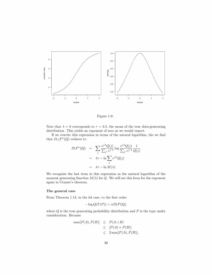
j jP (j) = τ . The distribu-tion P ∗ is called a twisted distribution and we’ll see other examples of this inconnection with Stein’s theorem. In Figure 1.4 we consider tossing a fair dice.Therefore, j = 6 in the above notation. In the figure, we plot first the relation-ship between λ and τ , and then the minimized KL divergence as a function of λ.

29

−2 −1 0 1 2

2

3

4

5

lambda

cons

trai

nt v

alue

−2 −1 0 1 2

−1.0

−0.8

−0.6

−0.4

−0.2

0.0

lambda

−D

(P*|

|Q)

Figure 1.9:

Note that λ = 0 corresponds to τ = 3.5, the mean of the true data-generatingdistribution. This yields an exponent of zero as we would expect.

If we rewrite this expression in terms of the natural logarithm, the we findthat De(P ∗‖Q) reduces to

D(P ∗‖Q) =∑

j

ejλQ(j)∑

j′ ej′λlog

ejλQ(j)∑

j′ ej′λ

1

Q(j)

= λτ − ln∑

j

ejλQ(j)

= λτ − lnM(λ)

We recognize the last term in this expression as the natural logarithm of themoment generating function M(λ) for Q. We will see this form for the exponentagain in Cramer’s theorem.

The general case

From Theorem 1.13, in the iid case, to the first order

− logQ(T (P )) = nD(P ||Q),

where Q is the true generating probability distribution and P is the type underconsideration. Because

max[P (A), P (B)] ≤ P (A ∪B)

≤ [P (A) + P (B)]

≤ 2 max[P (A), P (B)],

30

on a log scale, we have for all practical purposes (since for rare events, thelog probabilities are negatively large and factor 2 becomes negligible on the logscale),

logP (A ∪B) ≈ max[logP (A), logP (B)];

or− logP (A ∪B) ≈ min[− logP (A),− logP (B)];

If the rare event E of interest is a union of type classes, then

− logQn(E) ≈ nminP∈ED(P ||Q),

where Qn is the product measure based on Q.This can be interpreted as follows. If we want to calculate the probability

of a “rare” event E in a “large” experiment under a model Q, then all we haveto do is to find an appropriate model P under which the event is “natural” ornormal and then

− logQn(E) ≈ “size factor”D(P ||Q).

In the iid case, the size factor is n as we have seen. Sanov’s theoremSo the art of Large Deviations lies in the choice of the alternate model P .

The choice is by no means unique and a wrong choice can lead to a wronganswer. In our iid case, the good choice is obviously the distribution whichmatches the type in the observed sequence. In other situations, things are notalways clear. This is the same idea behind importance sampling for estimatingthe probability of a rare event through Monte Carlo simulations.

Example 1.5 (A Markov Alternate Model). Suppose we toss a fair coin ntimes independently of each other, and let X1, . . . , Xn denote the outcome. Wewould like to compute the probability q(n, k) that the number k of occurrencesof two consecutive heads is roughly ns, for some given 0 < s < 1. Here, wewould count the run HHH as two occurences of the event. We need to buildsome memory into the alternate model Pn so that consecutive occurrences of His natural under Pn. Toward this end, we consider the class of Markov modelswith transition matrix

P =

(

1 − β βα 1 − α

)

The stationary distribution π of this chain is given by π(H) = α/(α + β),and π(T ) = β/(α + β). (Recall that the stationary distrubution of P satisfiesPπ = π, so that a chain started in this distribution remains there in the sensethat P (Xn = H) = π(H) for all n.)

Therefore, the expected ratio of the number of consecutive heads to the totalrun n is then

α/(α+ β) × (1 − β).

So we should choose a model with

s =α(1 − β)

α+ β,

31

0.0 0.2 0.4 0.6 0.8 1.0

−0.8

−0.6

−0.4

−0.2

0.0

prop of HH

expo

nent

, g(x

)

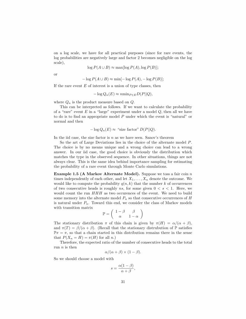
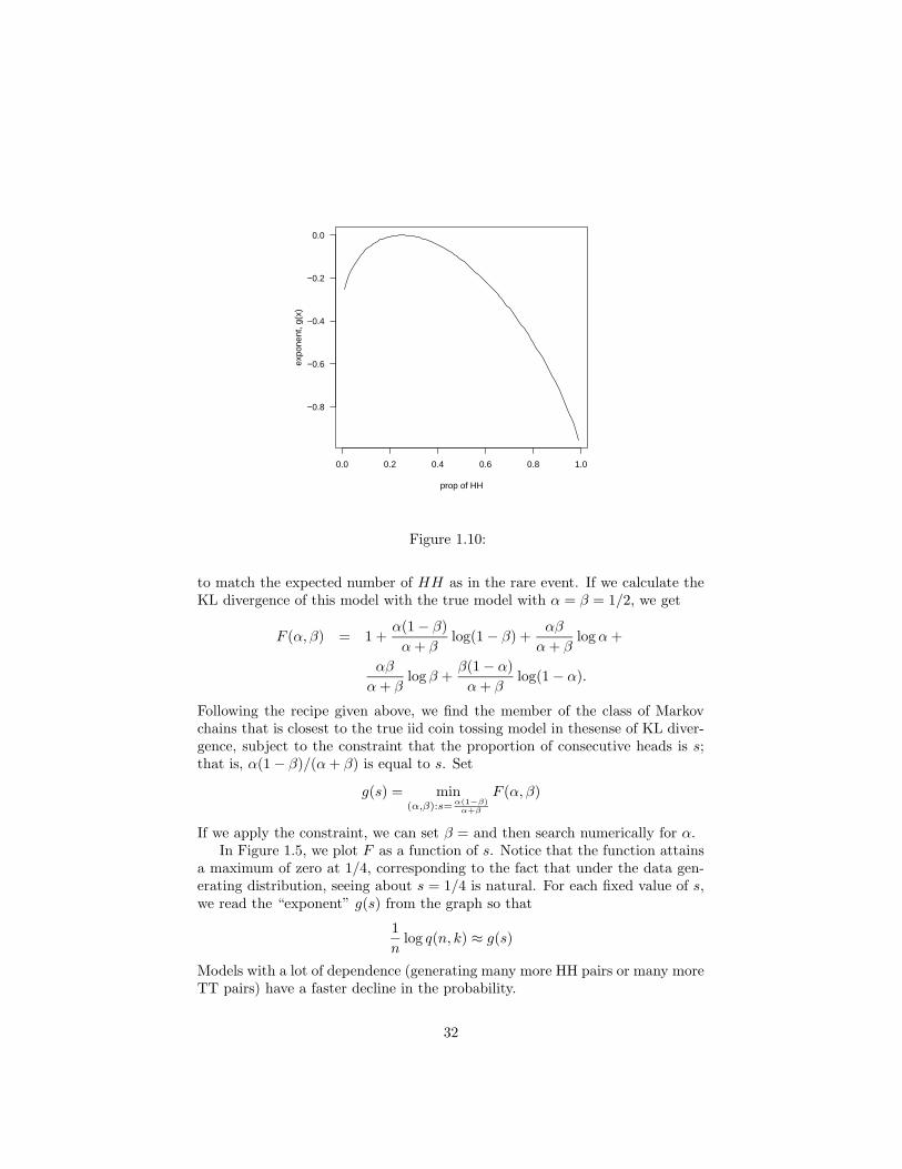
Figure 1.10:

to match the expected number of HH as in the rare event. If we calculate theKL divergence of this model with the true model with α = β = 1/2, we get

F (α, β) = 1 +α(1 − β)

α+ βlog(1 − β) +

αβ

α+ βlogα+

αβ

α+ βlog β +

β(1 − α)

α+ βlog(1 − α).

Following the recipe given above, we find the member of the class of Markovchains that is closest to the true iid coin tossing model in thesense of KL diver-gence, subject to the constraint that the proportion of consecutive heads is s;that is, α(1 − β)/(α+ β) is equal to s. Set

g(s) = min(α,β):s= α(1−β)

α+β

F (α, β)

If we apply the constraint, we can set β = and then search numerically for α.In Figure 1.5, we plot F as a function of s. Notice that the function attains

a maximum of zero at 1/4, corresponding to the fact that under the data gen-erating distribution, seeing about s = 1/4 is natural. For each fixed value of s,we read the “exponent” g(s) from the graph so that

1

nlog q(n, k) ≈ g(s)

Models with a lot of dependence (generating many more HH pairs or many moreTT pairs) have a faster decline in the probability.

32

The fact that this recipe works in more complex settings than those coveredby Sanov’s theorem can be explained somewhat intuitively.

Q(E) =

∫

E

dQ =

∫

E

dQ/dP dP.

If we pick P such that P (E) ≈ 1, then

logQ(E) − logP (E)

= log[1

P (E)

∫

E

dQ/dPdP ]

= log{ 1

P (E)

∫

E

exp[− log dP/dQ]dP}

≥ − 1

P (E)

∫

E

log[dP/dQ]dP

≈ −D(P ||Q)

Every P with P (E) ≈ 1 gives a lower bound and the particular P (·) =Q(· ∩E)/Q(E) gives the exact answer! But we are back to square 1. The trickor art is to choose a manageable class of alternate models so that the best lowerbound over the class matches the upper bound or gives the correct answer. Thisis problem-dependent as we have demonstrated through the Markov example.

Historically, the first LD result was not proved in terms of the KL divergence.Rather, moment generating functions were employed by Cramer (1938) to show

Theorem 1.14 (Cramer’s theorem). Let X1, .., Xn be iid random variables.Assume that the moment generating function

M(θ) = E[exp(θX])]

is finite for all θ ∈ R. Let φ(a) be the Legendre transform of ψ(θ) = logM(θ):

φ(a) = supθ

[aθ − ψ(θ)] = supθ

[aθ − logM(θ)].

φ(a) ≥ 0 and φ(a) = 0 if and only if a = E[X]. Then

P{X1 + ...+X − n

n∼ a] ≈ exp[−nφ(a)]

for a¬E(X).

As one might have guessed, the Legendre transform representation of theexponent can be equivalently expressed in terms of the KL divergence.

1.3.3 Stein’s Lemma in Hypothesis Testing

Hypothesis testing is one of the two major inference frameworks (the other be-ing estimation) in classifical statistical inference. Its most celebrated result is

33

the Neyman-Pearson Lemma obtained in the ??? which establishes the centralrole that the likelihood ratio was going to and is playing in hypothesis testing.The framework mimics the decision process to force a yes/no answer to the hy-pothesis being tested. Testing procedures are widely used in industry, especiallymandated by FDA regulations in pharmaceutical industry to report clinical trialresults. It is often used in health studies and the reports conform to the jargonssuch as statistical significant or highly statistically significant, which are oftentaken by the general public as ”significant” in the common sense, but ”scien-tifically proven” because of the appearence of the word “statistically”. This isvery unfortunately since all the evidence in terms of the probability of obtainingsomething more extreme than what has been observed or the p-value is calcu-lated assuming the dominate hypothsis is correct (which is often not the case)and the testing is done allowing itself to committ two types of errors, which arein the ideal case small but still non-zero.

Here we concentrate on the simplest case of telling two hypothesis or distri-butions apart.

Definition 10. Statistical Simple Hypothesis TestingLet X1, ..., Xn be iid with distribution Q and we test two simple hypotheses:

• H1 : Q = P1 (null hypothesis) vs

• H2 : Q = P2 (alternative hypothesis).

There are two typos of errors: false positive or type I error (H1 is wrong,but accepted) and false negative or type II error (H2 is true, but rejected).

Theorem 1.15 (Neyman-Pearson lemma). The optimal test given a type Ierror not larger than α is in the form of the likelihood ratio test, that is, acceptH1 when

An(T ) = {P1(xn)

P2(xn)> T}

where the cut-off value T is chosen such that

P1(Acn(T )) ≤ α.

Given a data string, the observed p-value of the test is the probability underthe null hypothesis that we would have observed some test statistics value whichis more extreme than the observed test statistics (e.g. likelihood ratio). p-valuesare comparable across different tests, while it is not always the case with teststatistics.

The optimality is defined in the sense that no other tests at this level with asmaller type II error or a smaller probability

P2(An(T ));

equivalently, there are not other tests with a larger power or a higher probability

P2(Acn(T )).

34

Example 1.6 (Gaussian location family).

The likelihood ratio test can be re-written in terms of KL divergences. Thatis,

P1(xn)

P2(xn)> T

is equivalent to

D(Pxn ||P2) −D(Pxn ||P1) >1

nlog T.

So the test is about how to choose type classes to form the acceptance region(or the rejection region). The boundary of the region is where the type classesare such that the differences between the KL divergences are a constant. LDcan now be employed to choose the cut-off value T in a heuristic manner.

Next, we calculate the best error exponent when one of the two types oferror goes to zero arbitrarily slowly.

Theorem 1.16 (Stein’s lemma). Assume D(P1||P2) <∞. Let the two typesof error are

αn = P1(Acn), βn = P2(An).

For 0 < ε < 1/2, define

βεn = minAn⊂Xn,αn<εβn.

Then

limε→0

limn→∞

1

nlog βε

n = −D(P1||P2).

One would like to make both types of error go to zero, at least as the samplesize n increases. The rates in Stein’s Lemma tell us that, for this to happen,it is necessary to make the two hypotheses apart at least by 1/n, or makeD(P1||P2)n → ∞. In other words, we can not distinguish two distributionswhich are less than 1/

√n apart in

√D which acts in the scale of a ”distance”.

Here we do not assume any parametric models where it is well-known thatwe can not estimate an Euclidean parameter at a rate faster than 1/

√n in

Euclidean distance – which is the consequence of requiring the more essentialdistance between two distributions to be larger than 1/

√n.

1.4 Joint entropy, conditional entropy, and mu-

tual information

For a pair of random variables (X,Y ), its (joint) entropy is easily defined as

Definition 11 (Joint Entropy). The joint entropy H(X,Y ) of a pair of dis-crete random variables (X,Y ) with a joint distribution P (x, y) is

H(X,Y ) = −∑

x∈X

∑

y∈Y

P (x, y) logP (x, y) = −E logP (X,Y ) (1.44)

35

When side information X, which is dependent on Y , is available at no costor little cost, it is better to use for the compression of the variable of interestY . This is the case in distributed compression and predictive coding.

For the next definition, we let P (y|x) denote the conditional distribution ofY given X = x.

Definition 12 (Conditional Entropy). Let (X,Y ) have the joint distributionfunction P (x, y). Then the conditional entropy is defined to be

H(Y |X) =∑

x∈X

P (x)H(Y |X = x) (1.45)

= −∑

x∈X

P (x)∑

y∈Y

P (y|x) logP (y|x) (1.46)

= −∑

x∈X

∑

y∈Y

P (x, y) logP (y|x) (1.47)

= −E logP (Y |X) (1.48)

Theorem 1.17 (Chain rule for entropy).

H(X,Y ) = H(X) +H(Y |X) (1.49)

Proof.

H(X,Y ) = −∑

x∈X

∑

y∈Y

P (x, y) logP (x, y) (1.50)

= −∑

x∈X

∑

y∈Y

P (x, y) logP (x)P (y|x) (1.51)

= −∑

x∈X

∑

y∈Y

P (x, y) logP (x) −∑

x∈X

∑

y∈Y

P (x, y) logP (y|x)(1.52)

= −∑

x∈X

P (x) logP (x) −∑

x∈X

∑

y∈Y

P (x, y) logP (y|x) (1.53)

= H(X) +H(Y |X) (1.54)

Example 1.1 (Experiments with News Stories). For this example, weconsider all the stories from nytimes.com on September 15, 2003. All theentropy calculations are done in the unit of nat. This collection consists of76,018 words

• We then ran the so-called Brill’s part of speech tagger over the corpus,assigning each word one of 35 labels (noun, verb, adjective, etc.). If X isa word and Y is the part of speech, then H(X) = 7.2, H(Y ) = 2.8 andH(X,Y ) = 7.4.

36

• Next, if for each sentence, we let X and Y denote consecutive words inthe sentence, H(X) = 7.1, H(Y ) = 7.3 and H(X,Y ) = 10.1. (Note thatthe entropy of X is slightly less than the previous example; we have leftoff the last X in each sentence.)

• Finally, suppose we let X represent words again and Y an indicator ofwhich story the word belonged to. Our test sample has 116 stories. Then,H(X) = 7.2, H(Y ) = 4.7 and H(X,Y ) = 10.0. This means that cer-tain words appear only in certain stories, reducing the entropy more thanknowing the part of speech or the previous word.

Corollary 1.2.H(X,Y |Z) = H(X|Z) +H(Y |X,Z) (1.55)

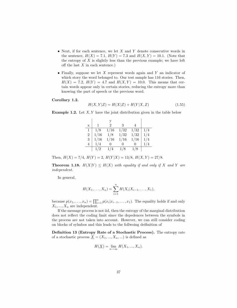
Example 1.2. Let X,Y have the joint distribution given in the table below

yx 1 2 3 41 1/8 1/16 1/32 1/32 1/42 1/16 1/8 1/32 1/32 1/43 1/16 1/16 1/16 1/16 1/44 1/4 0 0 0 1/4

1/2 1/4 1/8 1/8

Then, H(X) = 7/4, H(Y ) = 2, H(Y |X) = 13/8, H(X,Y ) = 27/8.

Theorem 1.18. H(X|Y ) ≤ H(X) with equality if and only if X and Y areindependent.

In general,

H(X1, . . . , Xn) =n

∑

i=1

H(Xi|Xi−1, . . . , X1),

because p(x1, . . . , xn) =∏n

i=1 p(xi|xi−1, . . . , x1). The equality holds if and onlyX1, ..., Xn are independent.

If the message process is not iid, then the entropy of the marginal distributiondoes not reflect the coding limit since the depedences between the symbols inthe process are not taken into account. However, we can still consider codingon blocks of sylmbos and this leads to the follwoing deifinition of

Definition 13 (Entropy Rate of a Stochastic Process). The entropy rateof a stochastic process X = (X1, ..., Xn, ...) is defined as

H(X) = limn→∞

H(X1, ..., Xn).

37

If we take the conditional view of the process or think about predictivecoding, then we arrive at an alternative definition for the entropy rate

H ′(X) = limn→∞

H(Xn|Xn−1, , ..., X1).

For stationary processes, these two definitions are equivalent fortunately

Theorem 1.19. For a stationary stochastic process on X , H(X) exists andequals H ′(X).

Proof. Since conditioning reduces entropy,

H(Xn+1|Xn, Xn−1, ..., X2, X1)

≤ H(Xn+1|Xn, Xn−1, ..., X2)

= H(Xn|Xn−1, Xn−2, ..., X1).

The last equality holds because of stationarity. Hence the sequence

H(Xn+1|Xn, Xn−1, ..., X2)

is non-negative and non-increasing so has a limit. By the chain rule on the jointentropy H(X1, ..., Xn), the averged joint entropy or H(X) is the average of theabove sequence and hence also shares the same limit.

Example 1.3 (Entropy rate of a stationary Markov process). If X is astationary Markov process of order 1,

H(Xn|Xn−1, ...., X1) = H(Xn|Xn−1) = H(X2|X1),

and the entropy rateH(X) = H(X2|X1).

If the Markov chain has only two states and with a transition probabilitymatrix (1− α, α;β, 1− β). Its stationary distribution is (α/(α+ β), β/(α+ β))and

H(X2|X1) =β

α+ βH(α) +

α

α+ βH(β).

***HW: Ch. 2: 4, 8, 9, 14; Ch. 12: 1, 2, 11.***

For a pair of random variables or a vector of them, an important question ison how much information they contain about each other; or how depedent theyare. Mutual information to be defined below answers this question naturallyand is the key ingredient in channel coding.

Definition 14 (Mutual Information). Let X,Y have a joint distributionP (x, y), and have marginal distributions P (x) and P (y). The mutual informa-tion I(X;Y ) is the relative entropy between the joint distribution of X,Y andthe product of their marginals; or rather, how far the joint distribution P (x, y)

38

is from independence. It therefore measures the dependence between the twovariables – the larger the mutual information, the more dependence they are.

I(X;Y ) =∑

x∈X

∑

y∈Y

P (x, y) logP (x, y)

P (x)P (y), (1.56)

I(X,Y ) = 0 if and only if X and Y are independent. The definition ofI(X,Y ) can easily be extended to the continuous case by replacing the summa-tion by an integration.

Using the definitions of mutual information and conditional entropy, we findthe following expression.

I(X;Y ) =∑

x∈X

∑

y∈Y

P (x, y) logP (x, y)

P (x)P (y) (1.57)

=∑

x∈X

∑

y∈Y

P (x, y) logP (y|x)

P (y)(1.58)

=∑

x∈X

∑

y∈Y

P (x, y) logP (y|x) −∑

x∈X

∑

y∈Y

P (x, y) logP (y) (1.59)

=∑

x∈X

∑

y∈Y

P (x, y) logP (y|x) −∑

y∈Y

P (y) logP (y) (1.60)

= H(Y ) −H(Y |X) (1.61)

Also, recall that H(Y ) − H(Y |X) = H(X) − H(X|Y ). Therefore, the mu-tual information records the reduction in uncertainty of X by knowing Y and,equivalently, the reduction in uncertainty in Y after knowing X. This is alsothe amount of information that X or Y contains about the other.

Example 1.4 (Bivariate Gaussian). Assume (X,Y ) are normal with meanzero and variance 1 and correlaction coefficient ρ. It is straghtforward to calcu-late that

I(X,Y ) = log2(1 − ρ2).

This is a monotonic transformation of the correlation coefficient which is theonly measure of dependence in the Gaussian case. The closer |ρ| to 1, the largerthe mutual information. The mutual information does not differetiate a positivecorrelation with a negative one, however.

Example 1.5 (Mutual information and document similarity). Here weconsider the use of mutual information in a text mining capacity.

It is easy to verify the chain rule for mutual information based on the chainrule for entropy and the entropy difference expression of mutual information:

I(X1, . . . , Xn;Y ) =

n∑

i=1

I(Xi, Y |Xi−1, . . . , X1)

.

39

D(p, q) is convex in pair (p, q)I(x, y) is concave in p(x) for fixed p(y|x)I(x, y) is convex in p(y|x) for fixed p(x)

1.4.1 Sufficiency

In the age of massive data collection, it is crucial to understand that manipula-tion of data doesn’t increase the information. This is stated most concisely inthe data processing inequality.

Theorem 1.20 (Data Processing Inequality). If X → Y → Z are Markov,then

I(X,Y ) ≥ I(X,Z). (1.62)

Proof. Using the chain rule on mutual information,

I(X;Z, Y ) = I(X,Z) + I(X,Y |Z) ≥ 0.

Similarly,I(X;Y, Z) = I(X,Y ) + I(X,Z|Y ) = I(X,Y )

since X and Z are independent given Y . Therefore

I(X,Y ) ≥ I(X,Z).

Corollary 1.3. For any function g, I(X,Y ) ≥ I(X, g(Y )).

Let fθ(x) be a parametric family. Our goal is to make inferences about θfrom sample x1, . . . , xn ∼ fθ(x1, ..., xn). A statistic T (x1, . . . , xn) is sufficient ifgiven T (X1, ..., Xn), θ and X are independent or the distribution of X1, ..., Xn

given T (X1, ..., Xn) is not dependent on θ.One can find a sufficient statistic in a straightforward manner by capitalizing

the factorization theorem:

Theorem 1.21 (Factorization Theorem). T is a sufficient statistic for fθ

if and only

fθ(x1, . . . , xn) = gθ(T (x1, . . . , xn))h(x1, . . . , xn|T (x1, . . . , xn)) (1.63)

where g and h are two nonnegative functions and h(x1, . . . , xn|T (x1, . . . , xn))does not depend on θ.

For example, if x1, . . . , xn are i.i.d. Gaussian with mean θ and variance 1,T (x) = x is sufficient.

Theorem 1.22 (Mutual Information and Sufficiency). T is a sufficientstatistic for fθ(X) iff

I(Θ, X) = I(Θ, T (X).

40

Proof. Since T is a mapping from X, we have

X → T (X),

which implies, by the data processing inequality, that

I(Θ, T (X)) ≤ I(Θ, X). (1.64)

On the other hand, T is a sufficient statistic,

Θ → T (x) → x,

soI(Θ, T (X)) ≥ I(Θ, X). (1.65)

Combining two inequalities gives I(Θ, T (X)) = I(Θ, X), so the mutual infor-mation of the parameter and the data is the same as mutual information of theparameter and the sufficient statistic. The converse???

Example 1.6 (Sufficient statistics). • X1, . . . , Xn i.i.d. Bernoulli(p). T (X) =∑n

i=1Xi.

• X1, . . . , Xn i.i.d. N(θ, σ2). T (X) = (∑

Xi,∑

X2i ), or equivalently (x, s2).

• X1, . . . , Xn i.i.d. Uniform(θ, θ+1). T (X) = (min(X1, . . . , Xn),max(X1, . . . , Xn)).

1.4.2 Fano’s inequality

Suppose X is the unknown and Y is our data. When H(X|Y ) is large, thereis much entropy or variability remaining about the unknown X even after wecollect the data Y and we can not hope to guess or estimate well X from Y .Fano’s inequality quantifies this observation, and it has two important appli-cations to be covered in the later lectures: proving the converse to Shannon’schannel coding theorem and giving lower bounds in minimax density estimation.

Theorem 1.23 (Fano’s Inequality). Suppose X → P (Y |X) → Y → X, thatis, X is an estimate of X based on Y . Let Pe = P (X 6= X) be the probabilityof error. Then

H(Pe) + Pe log(|X | − 1) ≥ H(X|Y ) (1.66)

where H(Pe) = −Pe logPe − (1 − Pe) log(1 − Pe). Note that if Pe = 0, thenH(X|Y ) = 0.

Proof. Let E = 1(X 6= X). Then

H(E,X|Y ) = H(X|Y ) +H(E|X,Y ) = H(X|Y )

(if you know X and Y , you know E, so H(E|X,Y ) = 0). On the other hand,one can also write

H(E,X|Y ) = H(E|Y ) +H(X|E, Y ). (1.67)

41

Now, H(E|Y ) ≤ H(E) = H(Pe), and

H(X|E, Y ) = P (E = 1)H(X|E = 1, Y ) + P (E = 0)H(X|E = 0, Y ).

If E = 0 and we know Y , we also know X, so H(X|E = 0, Y ) = 0. If E = 1,there are |X | − 1 possible values for X, so H(X|E, Y ) ≤ H(X) ≤ log(|X | − 1).Combining all the inequalities we get

H(X|Y ) ≤ H(E|Y ) + P (E = 1)H(X|E = 1, y) ≤ H(Pe) + Pe log(|X | − 1).(1.68)

Note: Fano’s inequality is sharp: let X ∈ {1, . . . ,m}, Y ≡ 1 = X, Pe =P (X 6= X). Let the distribution of X be p1 = 1 − Pe, p2 = · · · = pm = Pe

m−1 .Check that this achieves equality.

Corollary 1.4.

Pe ≥ 1 − I(X,Y ) + 1

H(X)(1.69)

Proof. 1+PeH(X) ≥ H(Pe)+PeH(X) ≥ H(X|Y ) = H(X|Y )−H(X)+H(X) =H(X) − I(X,Y ). Rearrange and get H(X)(Pe − 1) ≥ −I(X,Y ) − 1.

When X is uniform, H(X) = log(|X |), and Pe ≥ 1 − I(X,Y )+1log(|X |) .

1.4.3 Channel Capacity

Most communication channels (between people, callers and receivers over wiredtelephone lines or wireless phones) are noisy. The question is how much infor-mation can be transmitted through a noisy channel. Before Shannon’s 1948work, the common belief was that errors had to occur with a positive chance forany noisy channel. Shannon (1948) proved it possible to transmit without errorsin the limit when the message size gets large. However, he had to (1) allow anarbitrarily small but non zero probability of error; (2) use the channel manytims in succession (blocks) to the law of large numbers kicks in; (3) employ arandom code book by looking at the average probility of error over randomlygenerated block books to prove the existence of at least one good code book.

Definition 15 (Discrete Channel). A discrete channel is characterized by,for any given input x ∈ a finite alphabet X , a conditional distribution p(·|x) ona finite alphabet Y . The channel is said to be memoryless if

p(x1, ..., xn; y1, ..., yn) =n

∏

i=1

p(yi|xi)p(xi).

A good channel’s output or data yn should contain much information aboutthe input or unknown xn. If we use mutual information to capture this observa-tion, we should define the capacity of a channel to be the maximum informationpossible between a pair of input and output. That is,

42

Definition 16 (Channel Capacity). The information channel capacity of adiscrete memoryless channel is

C = maxp(x)

I(X;Y ),

where the maximum is taken over all possible input distribution p.

There is a duality between source coding and channel coding. In the former,we remove redundancy in the data to reduce the storage needed; in the latter,we add redundancy to the data to combat the channel noise. Channel decod-ing is basically an estimation problem, but the difference with the statisticalestimatino problem lies in the fact that the unknowns or inputs to the channelcan be manipulated to our advantage in channel coding but not in statisticalestimation in general.

Example 1.7 (Binary symmetric channel with cross-over probabilityp).

C = 1 −H(p).

Maximum capacity is 1 when p = 0 or the channel is noiseless.

Example 1.8 (Erasure channel erasure probability α). Here the outputalphabet Y = {0, e, 1} where e for erasure.

C = 1 − α.

Maximum capacity is 1 when α = 0 or the channel has no erasure.

Theorem 1.24 (Properties of C). 1. C ≥ 0.

2. C ≤ log |X |.

3. C ≤ log |Y|.

Definition 17 ((M, n) Code). An (M,n) code for a channel consists of thefollowing

1. An index set {1, ..., N};

2. An encoding functionXn: {1, 2, ...,M} → X n, yielding codewordsXn(1), ..., Xn(M)which form the codebook.

3. A decoding functiong : Yn → {1, ...,M}.

For a given (M,n) code, we use λ(n) and P(n)e to denote the maximum

probability of error and the average probability of error respectively. That is,

λ(n) = maxi∈{1,...,M}

λi

43

whereλi = P (g(Y n)¬i|Xn = Xn(i)).

P (n)e =

1

M

∑

i

λi.

We often denote an (M,n) code as a (2nR, n) code with R = logM/n (bitsper transmission) being the rate of the code.

Theorem 1.25 (Shannon’s channel coding theorem). For a discrete mem-oryless channel, all rates below capacity C are achievable. Specifically, for everyrate R < C, there exists a sequence of (2nR, n) codes with maximum probabilityof error λ(n) going to zero as n → ∞. Conversely, any sequence of (2nR, n)codes with λ(n) → 0 must have R ≤ C.

Proof. Heuristics:We work with typical sequences or typical joint sequences. In the world of

typical sequences, things are roughly uniformly distributed. So counting doesthe job.

For any input distribution p(x), there are only about 2nH(X) typical se-quences. For each of these typical sequences as an input, there are approx-imately 2nH(Y |X) possible Y -sequences which are almost equally likely. Wewant to ensure that no two X-sequences produce the same Y output sequence.

The total number of possible (typical) Y -sequences is ≈ 2nH(Y ). This sethas to be divided into sets of size 2nH(Y |X) corresponding to the different inputX sequences. Hence the total number of disjoint sets is less than or equal to

2n(H(Y )−nH(Y |X) = 2nI(X,Y ).

If the rate R < C = max I(X,Y ), we could find an input distribution p∗

such that R < I(X∗, Y ) and we could map the index set of the code into thesedisjoint sets through the X-typical sequences under p∗. Because R is strictly lessthan I(X∗, Y ) this translates into much ”room” in the space of input sequencesto cushion the rigorousness of the above argument which can be formalized viaLLN for X and Y and (X,Y ). The mapping of the code index into typicalsequences under p∗ is formally done via the famous random coding argument.Decoding can be done using maximum likelhood and through the joint typicalsequences.

Converse:Intuitively, it is easy to see that

I(Xn, Y n) ≤ nC,

which can be proved via the chain rules of entropy and conditional entropy. Itsays that the channel capacity can not be increased if we use the memorylesschannel repeatedly.

Given any (2nR, n) code with its maximum prob. of error going to zero, itsaverage prob. of error goes to zero too.

44

Let W be a uniform random variable on the index set of the code {1, ..., 2nR}and W be the decoded index. Then

Pe = P (W 6= W ) → 0.

By Fano’s inequality,

Pe ≤ (H(W |Y n) − 1)/(nR),

since log |2nR| = nR.It follows that

nR = H(W ) = H(W |Y n) + I(W,Y n) ≤ nRPe + 1 + nC,

which implies thatPe > 1 − C/R − 1/(nR) > 0,

if R > C. This contradicts with Pe → 0. Hence R ≤ C.

1.4.4 Non-parametric minimax density estimation

After a few decades of successful parametric modeling, the need to leave partic-ular families of distributions was increased enough in the 60’s that a systematicstudy began of estimation procedures which do not rely on a parametric formof distributions. Presumably, this is because more data were collected but thescience or social science discipline iteself was not ready to suggest a parametricform either because of the lack of subject knowledge or because it was impos-sible due to the high noise to signal ratios in other fields rather than physicalsciences.

Given iid samples x1, ..., xn from a density f , here are two of the commonnonparametric density estimators:

• histogram density estimator

• kernel density estimator:

f(x) =1

nh

n∑

i=1

φ

(

x− xi

h

)

The first estimator has as long a history as the tabulation of data and the secondcan at least be traced back to the 60’s.

When there is no parametric form for the underlying density, Fisher’s Max-imum Likelihood theory cannot provide the fundamental limit on estimationefficiency. Other frameworks become necessary. It is known that if no con-straints are put on the underlying distribution, it is futile to study the questionof what is the best estimator since for any given rate αn going to zero as n tendsto infinity and any density estimator, there is always a density such that theestimation error under this density is slower than αn.

45

One successful formulation of nonparametric density estimation has been theminimax approach with regularity conditions imposed on all the densities in aparticular class to which the true density is assumed to belong. More precisely,let M be the class and we seek a procedure that gives the best performance forthe worst density in the class:

f∗ = arg minf

maxf∈M

Efd(f, f)

where d is a distance measure between densities.For example M could be the following Lipschitz class:

M = {f : f is on [0, 1], 0 < c0 ≤ f ≤ c1, |f ′| < c′} .

For smooth density function classes, the minimax risk usually converges to zeroat a rate n−α for some 0 < α < 1/2, which is slower than the usual paramet-ric rate of n−1/2. To be more precise, if the logarithm of the density has pcontinuous derivatives the rate is α = 2p/(2p+ 1).

Historically, the minimax optimal rates were obtained in two separate stages.For the lower bound, an intricate subclass was constructed and explicit riskcalculations were possible based on inequalities such as Assouad’s, Le Cam’sor Fano’s (cf. Yu, 1996). One popular trick was to build an subclass indexedby a hypercube with expanding dimensions by having local pertubations of auniform density function within the constraints of the class. Depending onthe pertubation is up or down, we get the hypercube subclass. For the upperbound, one tries different known density estimators such as histogram or kernelestimators to match the rates in the lower bounds. There was no systematicway of finding minimax optimal estimators.

Yang and Barron (1999) unified the calculations in the lower and upperbounds by introducing the use of KL divergence and associated inequalities.

Suppose we are given a density function class M with some smoothness prop-erties. Recall that we have seen the Hellinger distance and the KL-divergencebetween any two densities f and g (with respect to the Lebesque measure):

H(f, g) = (

∫

(√

f −√g)2dx)1/2.

D(f‖g) =

∫

f logf

gdx.

Assumption: D(f, g) � H2(f, g) when f and g are “close”, i.e., there existconstants A and A′ s.t.

AH2(f, g) ≤ D(f‖g) ≤ A′H2(f, g) when H2(f, g) ≤ ε.

D is very convenient to use in analysis because there are many informationtheory inequalities related to it, but it is not a distance. H, on the other hand,is a distance, so if the assumption holds, one can switch back and forth betweenD and H and take advantage of both.

46

The fundamental limit of estimation over M is determined by the metricentropy of the class which is the counterpart of dimension in the finite dimen-sional case. For a given distance d, there are two ways to define such an entropydepending on whether or not we are considering the covering entropy or thepacking entropy. For the covering entropy, we use the KL-divergence for tech-nical convenience; and for the packing entropy, we use the Hellinger distance totake advantage of its triangle inequality.

Definition 18 (Minimal covering number). of a set M, Nd(εn), is theminimum number of balls of radius (in terms of

√D) εn needed to cover M.

That is, given an εn-cover TD(εn) = {f1, ..., fK} with cardinality K = |TD(εn)|such that for any f ∈ M, there is an fi ∈ TD(εn) with the property thatD(f, fi) ≤ ε2n, we have ND(εn) ≤ K. VD(εn) = log(ND(εn)) is called the metricentropy.

Definition 19 (Maximum packing number). of a set M is the maximumnumber of balls of radius (in terms of H) εn that can be packed inside Msothat their centers are in M and the balls do not overlap.

Lemma 1.2 (Mixture of Product Measures as an Estimator). SupposeGD(εn) is a minimal cover of M at radius εn, let p be the mixture of the productmeasures of the centers in the cover:

p(xn) =1

ND(εn)

ND(εn)∑

i

fi(xn).

Then for any f ∈ M,

D(f(xn)||p(xn) ≤ VD(εn) + nε2n.

Moreover, the mixture density p(xn) is the Bayes estimator of f(xn) ∈ G(εn)with respect to the uniform prior on G(εn) and risk or loss function D. That is,

p(xn) = argminQonxn

1

ND

ND∑

i

D(fi(xn)||Q(xn)).

The same conclusion still holds when the prior is not uniform and G is anyarbitrary density set.

Proof. For a given f ∈ M, there is a fj in GD(εn) such that D(f ||fi) ≤ εn,obviously

1

ND(εn)

ND(εn)∑

i

fi(xn) ≤ 1

ND(εn)fj(xn).

Hence

47

D(f(xn)||p(xn)) = Ef{log f(xn)/[1

ND(εn)

ND(εn)∑

i

fi(xn)]}

≤ Ef log f(xn)/{ 1

ND(εn)fj(xn)}

= log |GD(εn)| +D(f(xn)||fj(xn)

= VD(εn) + nD(f ||fj)

= VD(εn) + nε2n.

For the second conclusion, let us prove it in the general case.For a set of densities fθ(x) indexed by θ and a prior density π(θ) on the set,

we want to show that

m(x) =

∫

fθ(x)π(theta)dθ = argminQ

∫

D(fθ||Q)π(θ)dθ.

That is, for any density Q, it suffices to show that

I =

∫

D(fθ||Q)π(θ)dθ −∫

D(fθ||m)π(θ)dθ ≥ 0.

Notice that

I =

∫ ∫

fθ(x) log[m(x)/Q(x)]dxπ(theta)dθ

=

∫

log[m(x)/Q(x)][

∫

fθ(x)π(theta)dθ]dx

=

∫

m(x) log[m(x)/Q(x)]dx

= D(m||Q) ≥ 0

.

Theorem 1.26 (Upper bound). Using the notations in the previous lemma,construct a marginal density using the mixture density on the n-tuples:

f(x) =1

n

n−1∑

i=0

p(xi+1 = x|xi) =1

n

n−1∑

i=0

fi,

where f =i= p(xi+1 = x|xi). Then for any f ∈ M,

Ef(xn)D(f ||f) ≤ 1

nV (εn) + ε2n.

48

Proof. For any f ∈ M, since D(p||q) is convex in the pair (p, q), and f is aconvex combination,

EfD(f ||f) ≤ Ef1

n

n−1∑

i=0

D(f ||fi)

=1

n

n−1∑

i=0

EfD(f ||fi)

=1

n

n−1∑

i=0

Ef log f(xi+1/p(xi+1|xi)

=1

nD(f(xn)||p(xn)

≤ VD(εn)/n+ ε2n, by Lemma 1.2 .

Theorem 1.27 (Lower bound). Let f be an estimate based on an i.i.d. sam-ple X1, . . . , Xn from f ∈ M. Then

minf

maxf∈M

EfH2(f, f) � min

fmaxf∈M

EfD(f‖f) ≥ ε2n/8

The proof follows from the following two lemmas and the assumption thatD(f ||g) and H2(f, g) are equivalent when f and g are close.

Lemma 1.3. Given a maximal packing net G′(εn), for any estimator f ,

maxf∈M

EfH2(f, f) ≥ (εn/2)2 max

f∈G′(εn)Pf{f 6= f}

where f = arg minf∈G(εn)H2(f , f).

Proof. First let us show that if f ∈ G(εn), then

{f 6= f} ⊂ {H(f, f) ≥ εn/2}.

By contradiction: if H(f, f) < εn/2, but f 6= f , then there exists f ′ ∈ G(εn)

such that H(f , f ′) < H(f , f) < εn/2 (recall that f is projection of f onto thenet G, and so since f is not equal f , there must be another function in the netthat is closer to f). But then by triangular inequality

H(f, f ′) ≤ H(f , f ′) +H(f , f) < εn,

which contradicts the packing property of the net, since both f and f ′ belongto G(εn).

From the above and from Markov inequality we get

Pf{f 6= f} ≤ Pf{H(f, f) ≥ εn/2} ≤ EfH2(f, f)

(εn/2)2,

49

and thereforeEfH

2(f, f) ≥ (εn/2)2Pf{f 6= f}.Since G(εn) ⊂ M, we get

maxf∈M

EfH2(f, f) ≥ max

f∈G(εn)EfH

2(f, f) ≥ (εn/2)2Pf{f 6= f}.

Lemma 1.4.max

f∈G(εn)Pf{f 6= f} ≥ 1/2.

Proof. Let Θ be uniform on G(εn) = {fi : i = 1, . . . , N(εn)}. The entropyH(Θ) = log(N(εn)) = V (εn). From the corollary to Fano’s inequality,

Pf (f 6= f) = Pe ≥ 1 − I(Θ, Xn) + 1

log(N(εn))

Note that Θ → fi → Xn, and

I(Θ, Xn) =

N(εn)∑

i=1

1

N(εn)

∫

fi(xn) log

fi(xn)

fεn(xn)

dxn

≤N(εn)∑

i=1

1

N(εn)

∫

fi(xn) log

fi(xn)

Q(xn)dxn

where

fεn(xn) =

N(εn)∑

i=1

1

N(εn)fi(x

n)

is the Bayes mixture density which minimizes the Kullback-Leibler divergenceD(f‖Q) for any other density Q(xn), hence the last inequality.

Take another net G(εn) such that for any f ∈ M there exists f ∈ G(εn)such that D(f‖f) ≤ ε2n. Define

Q(xn) =1

N(εn)

∑

G(εn)

fi(xn)

If we replace the last sum by just one term from G(εn), we get

logfi(x

n)

Q(xn)≤ log

fi(xn)

1N(εn) f(xn)

Take expectations:

Ef logfi(x

n)1

N(εn) f(xn)= logN(εn) +D(fi(x

n)‖f(xn)) ≤ V (εn) + nε2n

50

Plugging into Fano’s inequality and choosing εn such that V (εn)+nε2n +1 =V (εn)/2 we get

maxf∈G(εn)

Pf{f 6= f} ≥ 1 − V (εn) + nε2n + 1

V (εn)=

1

2.

If we choose εn = αn such that

V (αn) = nα2n,

then we obtain the optimal minimax rate α2n since the rates in the lower and

upper bounds would match with such a choice.

Example 1.9 (Lipschitz Class). For the Lipschitz class defined earlier, it canbe shown that

V (ε) = 1/ε.

It follows that the optimal rate is n−2/3 after verifyting that H2 and D areequivalent for all memebers of the class.

51