lecture notes: interest rate theory - eth zjteichma/lecture_notes_ir... · · 2011-01-03lecture...

Lecture Notes: Interest Rate Theory


Josef Teichmann

ETH Zurich

Fall 2010

J. Teichmann Lecture Notes: Interest Rate Theory


Foreword

Mathematical Finance

Basics on Interest Rate Modeling

Black formulas

Affine LIBOR Models

Markov Processes

The SABR model

HJM-models

References

Catalogue of possible questions for the oral exam

1 / 107


Foreword

In mathematical Finance we need processes

I which can model all stylized facts of volatility surfaces andtimes series (e.g. tails, stochastic volatility, etc)

I which are analytically tractable to perform efficient calibration.

I which are numerically tractable to perform efficient pricingand hedging.

2 / 107


Foreword

Goals

I Basic concepts of stochastic modeling in interest rate theory.

I ”No arbitrage” as concept and through examples.

I Concepts of interest rate theory like yield, forward rate curve,short rate.

I Spot measure, forward measures, swap measures and Black’sformula.

I Short rate models

I Affine LIBOR models

I Fundamentals of the SABR model

I HJM model

I Consistency and Yield curve estimation

3 / 107



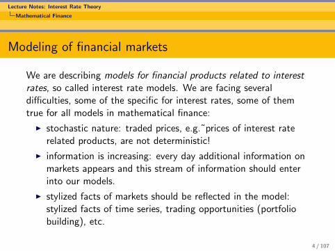
Modeling of financial markets

We are describing models for financial products related to interestrates, so called interest rate models. We are facing severaldifficulties, some of the specific for interest rates, some of themtrue for all models in mathematical finance:

I stochastic nature: traded prices, e.g.˜prices of interest raterelated products, are not deterministic!

I information is increasing: every day additional information onmarkets appears and this stream of information should enterinto our models.

I stylized facts of markets should be reflected in the model:stylized facts of time series, trading opportunities (portfoliobuilding), etc.

4 / 107



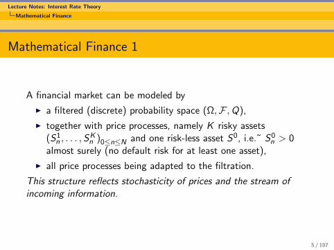
Mathematical Finance 1

A financial market can be modeled by

I a filtered (discrete) probability space (Ω,F ,Q),

I together with price processes, namely K risky assets(S1

n , . . . ,SKn )0≤n≤N and one risk-less asset S0, i.e.˜ S0

n > 0almost surely (no default risk for at least one asset),

I all price processes being adapted to the filtration.

This structure reflects stochasticity of prices and the stream ofincoming information.

5 / 107



A portfolio is a predictable process φ = (φ0n, . . . , φ

Kn )0≤n≤N , where

φin represents the number of risky assets one holds at time n. Thevalue of the portfolio Vn(φ) is

Vn(φ) =K∑i=0

φinS in.

6 / 107



Mathematical Finance 2

Self-financing portfolios φ are characterized through the condition

Vn+1(φ)− Vn(φ) =K∑i=0

φin+1(S in+1 − S i

n),

for 0 ≤ n ≤ N − 1, i.e.˜changes in value come from changes inprices, no additional input of capital is required and noconsumption is allowed.

7 / 107



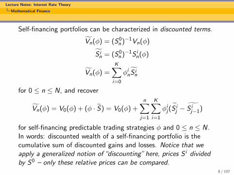
Self-financing portfolios can be characterized in discounted terms.

Vn(φ) = (S0n )−1Vn(φ)

S in = (S0

n )−1S in(φ)

Vn(φ) =K∑i=0

φinS in

for 0 ≤ n ≤ N, and recover

Vn(φ) = V0(φ) + (φ · S) = V0(φ) +n∑

j=1

K∑i=1

φij(S ij − S i

j−1)

for self-financing predictable trading strategies φ and 0 ≤ n ≤ N.In words: discounted wealth of a self-financing portfolio is thecumulative sum of discounted gains and losses. Notice that weapply a generalized notion of “discounting” here, prices S i dividedby S0 – only these relative prices can be compared.

8 / 107



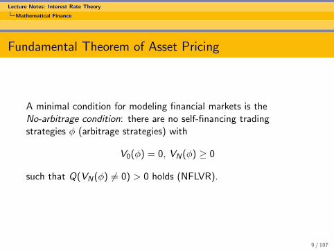
Fundamental Theorem of Asset Pricing

A minimal condition for modeling financial markets is theNo-arbitrage condition: there are no self-financing tradingstrategies φ (arbitrage strategies) with

V0(φ) = 0, VN(φ) ≥ 0

such that Q(VN(φ) 6= 0) > 0 holds (NFLVR).

9 / 107



Fundamental Theorem of Asset Pricing

A minimal condition for financial markets is the no-arbitragecondition: there are no self-financing trading strategies φ(arbitrage strategies) with V0(φ) = 0, VN(φ) ≥ 0 such thatQ(VN(φ) 6= 0) > 0 holds (NFLVR).In other words the set

K = VN(φ)|V0(φ) = 0, φ self-finanancing

intersects L0≥0(Ω,F ,Q) only at 0,

K ∩ L0≥0(Ω,F ,Q) = 0.

10 / 107



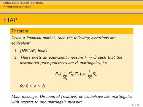
FTAP

Theorem

Given a financial market, then the following assertions areequivalent:

1. (NFLVR) holds.

2. There exists an equivalent measure P ∼ Q such that thediscounted price processes are P-martingales, i.e.

EP(1

S0N

S iN |Fn) =

1

S0n

S in

for 0 ≤ n ≤ N.

Main message: Discounted (relative) prices behave like martingaleswith respect to one martingale measure.

11 / 107



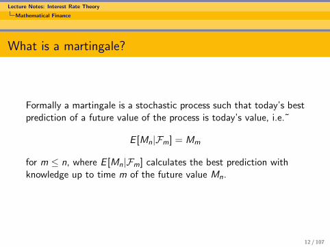
What is a martingale?

Formally a martingale is a stochastic process such that today’s bestprediction of a future value of the process is today’s value, i.e.˜

E [Mn|Fm] = Mm

for m ≤ n, where E [Mn|Fm] calculates the best prediction withknowledge up to time m of the future value Mn.

12 / 107



Random walks and Brownian motions are well-known examples ofmartingales. Martingales are particularly suited to describe(discounted) price movements on financial markets, since theprediction of future returns is 0.

13 / 107



Pricing rules

(NFLVR) also leads to arbitrage-free pricing rules. Let X be thepayoff of a claim X paying at time N, then an adapted stochasticprocess π(X ) is called pricing rule for X if

I πN(X ) = X .

I (S0, . . . ,SN , π(X )) is free of arbitrage.

This is equivalent to the existence of one equivalent martingalemeasure P such that

EP

( X

S0N

|Fn

)=πn(X )

S0n

holds true for 0 ≤ n ≤ N.

14 / 107



Proof of FTAP

The proof is an application of separation theorems for convex sets:we consider the euclidean vector space L2(Ω,R) of real valuedrandom variables with scalar product

〈X ,Y 〉 = E (XY ).

Then the convex set K does not intersect the positive orthantL2≥0(Ω,R), hence we can find a vector R, which is strictly positive

and which is orthogonal to all elements of K (draw it!). We arefree to choose E (R) = 1. We can therefore define a measure Q onF via

Q(A) = E (1AR)

and this measure has the same nullsets as P by strict positivity.

15 / 107



Proof of FTAP

By construction we have that every element of K has vanishingexpectation with respect to Q since R is orthogonal to K . Since Kconsists of all stochastic integrals with respect to S we obtain byDoob’s optional sampling that S is a Q-martingale, whichcompletes the proof.

16 / 107



One step binomial model

We model one asset in a zero-interest rate environment just beforethe next tick. We assume two states of the world: up, down. Theriskless asset is given by S0 = 1. The risky asset is modeled by

S10 = S0, S1

1 = S0 ∗ u > S0 or S11 = S0 ∗ 1/u = S0 ∗ d

where the events at time one appear with probability q and 1− q(”physical measure”). The martingale measure is apparently giventhrough u ∗ p + (1− p)d = 1, i.e.˜ p = 1−d

u−d .Pricing a European call option at time one in this setting leads tofair price

E [(S11 − K )+] = p ∗ (S0u − K )+ + (1− p) ∗ (S0d − K )+.

17 / 107



Black-Merton-Scholes model 1

We model one asset with respect to some numeraire by anexponential Brownian motion. If the numeraire is a bank accountwith constant rate we usually speak of the Black-Merton-Scholesmodel, if the numeraire some other traded asset, for instance azero-coupon bond, we speak of Black’s model. Let us assume thatS0 = 1, then

S1t = S0 exp(σBt −

σ2t

2)

with respect to the martingale measure P. In the physical measureQ a drift term is added in the exponent, i.e.˜

S1t = S0 exp(σBt −

σ2t

2+ µt).

18 / 107



Black-Merton-Scholes model 2

Our theory tells that the price of a European call option on S1 attime T is priced via

E [(S1T − K )+] = S0Φ(d1)− KΦ(d2)

yielding the Black-Scholes formula, where Φ is the cumulativedistribution function of the standard normal distribution and

d1,2 =log S0

K ±σ2T

2

σ√

T.

Notice that this price corresponds to the value of a portfoliomimicking the European option at time T .

19 / 107



Some general facts

I Fixed income markets (i.e. interest rate related products)form a large scale market in any major economy, for instanceswaping fixed against floating rates.

I Fixed income markets, in contrast to stock markets, consist ofproducts with a finite life time (i.e. zero coupon bonds) andstrong dependencies (zero coupon bonds with close maturitiesare highly dependent).

I mathematically highly challenging structures can appear ininterest rate modeling.

20 / 107



Interest Rate mechanics 1

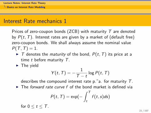
Prices of zero-coupon bonds (ZCB) with maturity T are denotedby P(t,T ). Interest rates are given by a market of (default free)zero-coupon bonds. We shall always assume the nominal valueP(T ,T ) = 1.

I T denotes the maturity of the bond, P(t,T ) its price at atime t before maturity T .

I The yield

Y (t,T ) = − 1

T − tlog P(t,T )

describes the compound interest rate p.˜a. for maturity T .I The forward rate curve f of the bond market is defined via

P(t,T ) = exp(−∫ T

tf (t, s)ds)

for 0 ≤ t ≤ T .21 / 107



Interest rate models

An interest rate model is a collection of adapted stochasticprocesses (P(t,T ))0≤t≤T on a stochastic basis (Ω,F ,P) withfiltration (Ft)t≥0 such that

I P(T ,T ) = 1 (nominal value is normalized to one),

I P(t,T ) > 0 (default free market)

holds true for 0 ≤ t ≤ T .

22 / 107



Interest Rate mechanics 2

I The short rate process is given through Rt = f (t, t) for t ≥ 0defining the “bank account process”

(B(t))t≥0 := (exp(

∫ t

0Rsds))t≥0.

I The existence of forward rates and short rates is anassumption on regularity with respect to maturity T . Asufficient conditions for the existence of Yields and forwardrates is that bond prices are continuously differentiable withrespect with T .

23 / 107



I Notice that the market to model consists only of ZCB,apparently the bank account has to be formed from ZCB via aroll-over-portfolio.

I The roll-over-portfolio consists of investing one unit ofcurrency into a T1-ZCB, then reinvesting at time T1 into aT2-ZCB, etc. Given an increasing sequenceT = 0 < T1 < T2 < . . . yields the wealth at time t

BT(t) =∏Ti≤t

1

P(t,Ti )

I We speak of a (generalized) “bank account process” of BT

allows for limiting – this is in particular the case of we have ashort rate process with some integrability properties.

24 / 107



Simple forward rates – LIBOR rates

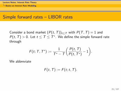
Consider a bond market (P(t,T ))t≤T with P(T ,T ) = 1 andP(t,T ) > 0. Let t ≤ T ≤ T ∗. We define the simple forward ratethrough

F (t; T ,T ∗) :=1

T ∗ − T

(P(t,T )

P(t,T ∗)− 1

).

We abbreviate

F (t,T ) := F (t; t,T ).

25 / 107



Apparently P(t,T ∗)F (t; T ,T ∗) is the fair value at time t of acontract paying F (T ,T ∗) at time T ∗, in the sense that there is aself-financing portfolio with value P(t,T ∗)F (t; T ,T ∗) at time tand value F (T ,T ∗) at time T ∗.

26 / 107



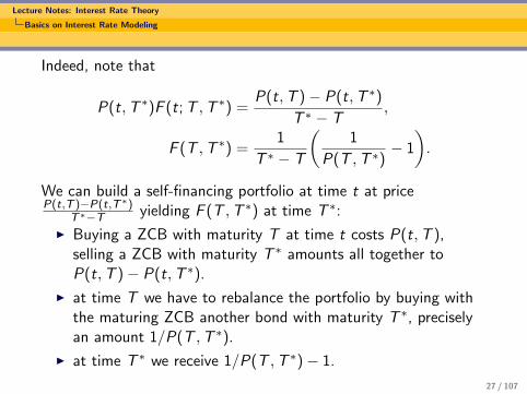
Indeed, note that

P(t,T ∗)F (t; T ,T ∗) =P(t,T )− P(t,T ∗)

T ∗ − T,

F (T ,T ∗) =1

T ∗ − T

(1

P(T ,T ∗)− 1

).

We can build a self-financing portfolio at time t at priceP(t,T )−P(t,T∗)

T∗−T yielding F (T ,T ∗) at time T ∗:

I Buying a ZCB with maturity T at time t costs P(t,T ),selling a ZCB with maturity T ∗ amounts all together toP(t,T )− P(t,T ∗).

I at time T we have to rebalance the portfolio by buying withthe maturing ZCB another bond with maturity T ∗, preciselyan amount 1/P(T ,T ∗).

I at time T ∗ we receive 1/P(T ,T ∗)− 1.

27 / 107



Caps

In the sequel, we fix a number of future dates

T0 < T1 < . . . < Tn

with Ti − Ti−1 ≡ δ.Fix a rate κ > 0. At time Ti the holder of the cap receives

δ(F (Ti−1,Ti )− κ)+.

Let t ≤ T0. We write

Cpl(t; Ti−1,Ti ), i = 1, . . . , n

for the time t price of the ith caplet, and

Cp(t) =n∑

i=1

Cpl(t; Ti−1,Ti )

for the time t price of the cap.28 / 107



Floors

At time Ti the holder of the floor receives

δ(κ− F (Ti−1,Ti ))+.

Let t ≤ T0. We write

Fll(t; Ti−1,Ti ), i = 1, . . . , n

for the time t price of the ith floorlet, and

Fl(t) =n∑

i=1

Fll(t; Ti−1,Ti )

for the time t price of the floor.

29 / 107



Swaps

Fix a rate K and a nominal N. The cash flow of a payer swap atTi is

(F (Ti−1,Ti )− K )δN.

The total value Πp(t) of the payer swap at time t ≤ T0 is

Πp(t) = N

(P(t,T0)− P(t,Tn)− Kδ

n∑i=1

P(t,Ti )

).

The value of a receiver swap at t ≤ T0 is

Πr (t) = −Πp(t).

The swap rate Rswap(t) is the fixed rate K which givesΠp(t) = Πr (t) = 0. Hence

Rswap(t) =P(t,T0)− P(t,Tn)

δ∑n

i=1 P(t,Ti ), t ∈ [0,T0].

30 / 107



Swaptions

A payer (receiver) swaption is an option to enter a payer (receiver)swap at T0. The payoff of a payer swaption at T0 is

Nδ(Rswap(T0)− K )+n∑

i=1

P(T0,Ti ),

and of a receiver swaption

Nδ(K − Rswap(T0))+n∑

i=1

P(T0,Ti ).

31 / 107



Note that it is very cumbersome to write models which areanalytically tractable for both swaptions and caps/floors.

I Black’s model is a lognormal model for one bond price withrespect to a particular numeraire. If we change the numerairethe lognormal property gets lost.

I The change of numeraire between swap and forward measuresis a rational function, which usually destroys analytictractability properties of given models.

32 / 107



Spot measure

The spot measure is defined as a martigale measure for the ZCBprices discounted by their own bank account process

P(t,T )

B(t)

for T ≥ 0. This leads to the following fundamental formula ofinterest rate theory

P(t,T ) = E (exp(−∫ T

tRsds))|Ft)

for 0 ≤ t ≤ T with respect to the spot measure.

33 / 107



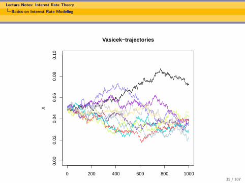
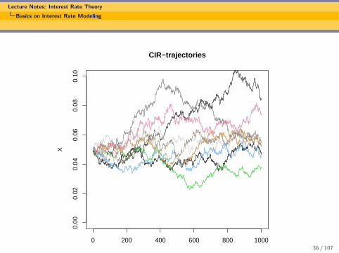
Short rate models

We can assume several dynamics with respect to the spot measure:

I Vasicek model: dRt = (βRt + b)dt + 2αdWt .

I CIR model: dRt = (βRt + b)dt + 2α√

(Rt)dWt .

In the following two slides typical Vasicek and CIR trajectories aresimulated.

34 / 107



0 200 400 600 800 1000

0.00

0.02

0.04

0.06

0.08

0.10

Index

XVasicek−trajectories

35 / 107



0 200 400 600 800 1000

0.00

0.02

0.04

0.06

0.08

0.10

Index

XCIR−trajectories

36 / 107



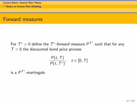
Forward measures

For T ∗ > 0 define the T ∗-forward measure PT∗such that for any

T > 0 the discounted bond price process

P(t,T )

P(t,T ∗), t ∈ [0,T ]

is a PT∗-martingale.

37 / 107



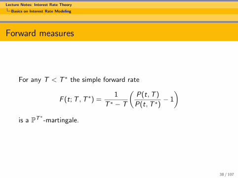
Forward measures

For any T < T ∗ the simple forward rate

F (t; T ,T ∗) =1

T ∗ − T

(P(t,T )

P(t,T ∗)− 1

)is a PT∗

-martingale.

38 / 107



For any time T derivative X ∈ FT we have that the fair value via“martingale pricing” is given through

P(t,T )ET [X |Ft ].

The fair price of the ith caplet is therefore given by

Cpl(t; Ti−1,Ti ) = δP(t,Ti )ETi [(F (Ti−1,Ti )− κ)+|Ft ].

By the martingale property we obtain therefore

ETi [F (Ti−1,Ti )|Ft ] = F (t; Ti−1,Ti ),

what was proved by trading arguments before.

39 / 107



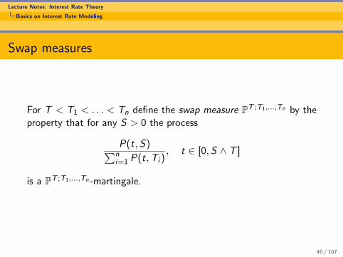
Swap measures

For T < T1 < . . . < Tn define the swap measure PT ;T1,...,Tn by theproperty that for any S > 0 the process

P(t,S)∑ni=1 P(t,Ti )

, t ∈ [0, S ∧ T ]

is a PT ;T1,...,Tn-martingale.

40 / 107



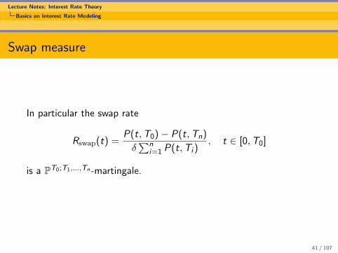
Swap measure

In particular the swap rate

Rswap(t) =P(t,T0)− P(t,Tn)

δ∑n

i=1 P(t,Ti ), t ∈ [0,T0]

is a PT0;T1,...,Tn-martingale.

41 / 107



For any X ∈ FT we have that the fair price is given by( n∑i=1

P(t,Ti ))ET0;T1,...,Tnt [X ].

42 / 107


Black formulas

I Black formulas are applications of the lognormalBlack-Scholes theory to model LIBOR rates or swap rates.

I Black formulas are not constructed from one model oflognormal type for all modeled quantities (LIBOR rates, swaprates, forward rates, etc).

I Generically only of the following quantities is lognormal withrespect to one particular measure: one LIBOR rate or oneswap rate, each for a certain tenor.

43 / 107


Black formulas

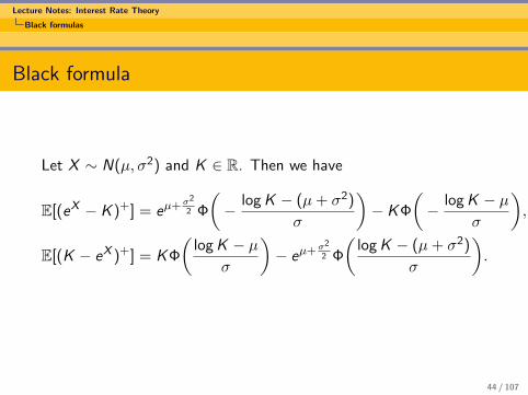
Black formula

Let X ∼ N(µ, σ2) and K ∈ R. Then we have

E[(eX − K )+] = eµ+σ2

2 Φ

(− log K − (µ+ σ2)

σ

)− KΦ

(− log K − µ

σ

),

E[(K − eX )+] = KΦ

(log K − µ

σ

)− eµ+σ2

2 Φ

(log K − (µ+ σ2)

σ

).

44 / 107


Black formulas

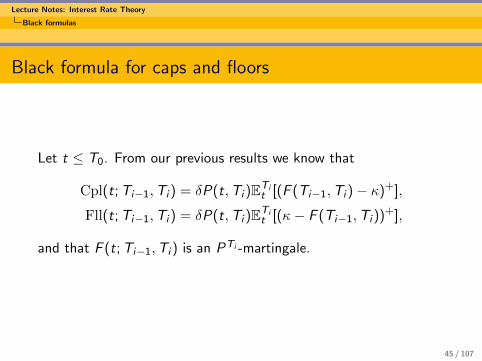
Black formula for caps and floors

Let t ≤ T0. From our previous results we know that

Cpl(t; Ti−1,Ti ) = δP(t,Ti )ETit [(F (Ti−1,Ti )− κ)+],

Fll(t; Ti−1,Ti ) = δP(t,Ti )ETit [(κ− F (Ti−1,Ti ))+],

and that F (t; Ti−1,Ti ) is an PTi -martingale.

45 / 107


Black formulas

Black formula for caps and floors

We assume that under PTi the forward rate F (t; Ti−1,Ti ) is anexponential Brownian motion

F (t; Ti−1,Ti ) = F (s; Ti−1,Ti )

exp

(− 1

2

∫ t

sλ(u,Ti−1)2du +

∫ t

sλ(u,Ti−1)dW Ti

u

)for s ≤ t ≤ Ti−1, with a function λ(u,Ti−1).

46 / 107


Black formulas

We define the volatility σ2(t) as

σ2(t) :=1

Ti−1 − t

∫ Ti−1

tλ(s,Ti−1)2ds.

The PTi -distribution of log F (Ti−1,Ti ) conditional on Ft isN(µ, σ2) with

µ = log F (t; Ti−1,Ti )−σ2(t)

2(Ti−1 − t),

σ2 = σ2(t)(Ti−1 − t).

In particular

µ+σ2

2= log F (t; Ti−1,Ti ),

µ+ σ2 = log F (t; Ti−1,Ti ) +σ2(t)

2(Ti−1 − t).

47 / 107


Black formulas

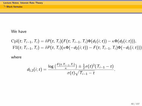
We have

Cpl(t; Ti−1,Ti ) = δP(t,Ti )(F (t; Ti−1,Ti )Φ(d1(i ; t))− κΦ(d2(i ; t))),

Fll(t; Ti−1,Ti ) = δP(t,Ti )(κΦ(−d2(i ; t))− F (t; Ti−1,Ti )Φ(−d1(i ; t))),

where

d1,2(i ; t) =log(F (t;Ti−1,Ti )

κ

)± 1

2σ(t)2(Ti−1 − t)

σ(t)√

Ti−1 − t.

48 / 107


Black formulas

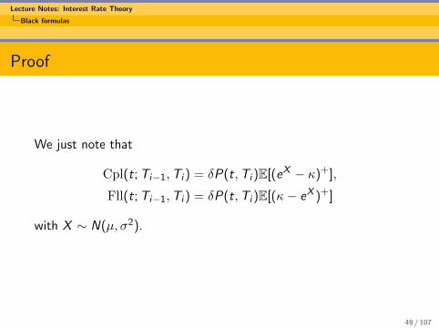
Proof

We just note that

Cpl(t; Ti−1,Ti ) = δP(t,Ti )E[(eX − κ)+],

Fll(t; Ti−1,Ti ) = δP(t,Ti )E[(κ− eX )+]

with X ∼ N(µ, σ2).

49 / 107


Black formulas

Black’s formula for swaptions

Let t ≤ T0. From our previous results we know that

Swptp(t) = Nδn∑

i=1

P(t,Ti )EPT0;T1,...,Tn

t [(Rswap(T0)− K )+],

Swptr (t) = Nδn∑

i=1

P(t,Ti )EPT0;T1,...,Tn

t [(K − Rswap(T0))+],

and that Rswap is an PT0;T1,...,Tn-martingale.

50 / 107


Black formulas

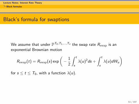
Black’s formula for swaptions

We assume that under PT0;T1,...,Tn the swap rate Rswap is anexponential Brownian motion

Rswap(t) = Rswap(s) exp

(− 1

2

∫ t

sλ(u)2ds +

∫ t

sλ(u)dWu

)for s ≤ t ≤ T0, with a function λ(u).

51 / 107


Black formulas

We define the implied volatility σ2(t) as

σ2(t) :=1

T0 − t

∫ T0

tλ(s)2ds.

The PT0;T1,...,Tn-distribution of log Rswap(T0) conditional on Ft isN(µ, σ2) with

µ = log Rswap(t)− σ2(t)

2(T0 − t),

σ2 = σ2(t)(T0 − t).

In particular

µ+σ2

2= log Rswap(t),

µ+ σ2 = log Rswap(t) +σ2(t)

2(T0 − t).

52 / 107


Black formulas

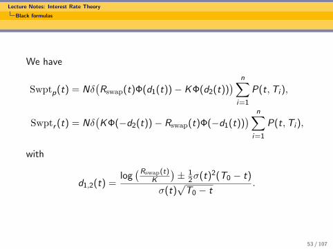
We have

Swptp(t) = Nδ(Rswap(t)Φ(d1(t))− KΦ(d2(t))

) n∑i=1

P(t,Ti ),

Swptr (t) = Nδ(KΦ(−d2(t))− Rswap(t)Φ(−d1(t))

) n∑i=1

P(t,Ti ),

with

d1,2(t) =log(Rswap(t)

K

)± 1

2σ(t)2(T0 − t)

σ(t)√

T0 − t.

53 / 107


Affine LIBOR Models

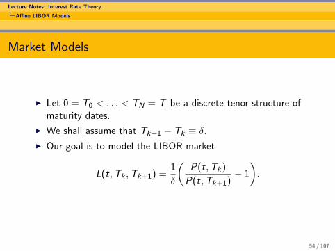
Market Models

I Let 0 = T0 < . . . < TN = T be a discrete tenor structure ofmaturity dates.

I We shall assume that Tk+1 − Tk ≡ δ.

I Our goal is to model the LIBOR market

L(t,Tk ,Tk+1) =1

δ

(P(t,Tk)

P(t,Tk+1)− 1

).

54 / 107


Affine LIBOR Models

Three Axioms

The following axioms are motivated by economic theory, arbitragepricing theory and applications:

I Axiom 1: Positivity of the LIBOR rates

L(t,Tk ,Tk+1) ≥ 0.

I Axiom 2: Martingale property under the correspondingforward measure

L(t,Tk ,Tk+1) ∈M(PTk+1).

I Axiom 3: Analytical tractability.

55 / 107


Affine LIBOR Models

Known Approaches

Here are some known approaches:

I Let L(t,Tk ,Tk+1) be an exponential Brownian motion. Thenanalytical tractability not completely satisfied (“Freezing thedrift”).

I Let P(t,Tk)P(t,Tk+1) be an exponential Brownian motion. Then

positivity of the LIBOR rates is not satisfied.

I We will study affine LIBOR models.

56 / 107


Affine LIBOR Models

Affine Processes

Let X = (Xt)0≤t≤T be a conservative, time-homogeneous,stochastically continuous process taking values in D = Rd

≥0.Setting

IT := u ∈ Rd : E[e〈u,XT 〉] <∞,

we assume that:

I 0 ∈ IT ;

I there exist functions φ : [0,T ]× IT → R andψ : [0,T ]× IT → Rd such that

E[e〈u,XT 〉] = exp(φt(u) + 〈ψt(u),X0〉)

for all 0 ≤ t ≤ T and u ∈ IT .

57 / 107


Affine LIBOR Models

Some Properties of Affine Processes

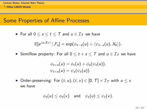
I For all 0 ≤ s ≤ t ≤ T and u ∈ IT we have

E[e〈u,XT 〉 | Fs ] = exp(φt−s(u) + 〈ψt−s(u),X0〉).

I Semiflow property: For all 0 ≤ t + s ≤ T and u ∈ IT we have

φt+s(u) = φt(u) + φs(ψt(u)),

ψt+s(u) = ψs(ψt(u)).

I Order-preserving: For (t, u), (t, v) ∈ [0,T ]× IT with u ≤ vwe have

φt(u) ≤ φt(v) and ψt(u) ≤ ψt(v).

58 / 107


Affine LIBOR Models

Constructing Martingales ≥ 1

For u ∈ IT we define Mu = (Mut )0≤t≤T as

Mut := exp(φT−t(u) + 〈ψT−t(u),Xt〉).

Then the following properties are valid:

I Mu is a martingale.

I For u ∈ Rd≥0 and X0 ∈ Rd

≥0 we have Mut ≥ 1.

59 / 107


Affine LIBOR Models

Constructing the Affine LIBOR Model

I We fix u1 > . . . > uN from IT ∩ Rd≥0 and set

P(t,Tk)

P(t,TN)= Muk

t , k = 1, . . . ,N.

I Obviously, we set

uN = 0⇔ P(0,TN)

P(0,TN)= 1.

60 / 107


Affine LIBOR Models

Positivity

Then we have

P(t,Tk)

P(t,Tk+1)= exp(Ak + 〈Bk ,Xt〉),

where we have defined

Ak := AT−t(uk , uk+1) := φT−t(uk)− φT−t(uk+1),

Bk := BT−t(uk , uk+1) := ψT−t(uk)− ψT−t(uk+1).

Note that Ak ,Bk ≥ 0 by the order-preserving property of φt(·) andψt(·). Thus, the LIBOR rates are positive:

L(t,Tk ,Tk+1) =1

δ

(P(t,Tk)

P(t,Tk+1)−1

)=

1

δ(exp(Ak + 〈Bk ,Xt〉)︸︷︷︸

≥1

−1) ≥ 0.

61 / 107


Affine LIBOR Models

Martingale Property

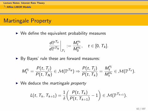
I We define the equivalent probability measures

dPTk

dPTN

∣∣∣∣Ft

:=Muk

t

Muk0

, t ∈ [0,Tk ].

I By Bayes’ rule these are forward measures:

Mujt =

P(t,Tj)

P(t,TN)∈M(PTN )⇒

P(t,Tj)

P(t,Tk)=

Mujt

Mukt∈M(PTk ).

I We deduce the martingale property

L(t,Tk ,Tk+1) =1

δ

(P(t,Tk)

P(t,Tk+1)− 1

)∈M(PTk+1).

62 / 107


Affine LIBOR Models

Analytical Tractability

I X is a time-homogeneous affine process under any forwardmeasure:

ETk [e〈v ,Xt〉] = exp(φkt (v) + 〈ψkt (v),X0〉).

I The functions φk and ψk are given by

φkt (v) := φt(ψT−t(uk) + v)− φt(ψT−t(uk)),

ψkt (v) := ψt(ψT−t(uk) + v)− ψt(ψT−t(uk)).

63 / 107


Affine LIBOR Models

Option Pricing

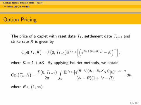
The price of a caplet with reset date Tk , settlement date Tk+1 andstrike rate K is given by

Cpl(Tk ,K ) = P(0,Tk+1)ETk+1

[(eAk+〈Bk ,XTk

〉 −K)+]

,

where K = 1 + δK . By applying Fourier methods, we obtain

Cpl(Tk ,K ) =P(0,Tk+1)

2π

∫R

ETk+1 [e(R−iv)(Ak+〈Bk ,XTk〉)]K1+iv−R

(iv − R)(1 + iv − R)dv ,

where R ∈ (1,∞).

64 / 107


Markov Processes

Definition of a Markov Process

I A family of adapted Rd -valued stochastic processes(X x

t )t≥0,x∈S is called time-homogenous Markov process with

state space S if for all s ≤ t and B ∈ B(Rd) we have

P(X xt ∈ B | Fs) = P(X y

t−s ∈ B)|y=Xs .

In particular Markov processes with state space S take valuesin S almost surely.

I We can define the associated Markov kernelsµs,t : Rd × B(Rd)→ [0, 1] with

µs,t(y ,B) = P(X yt−s ∈ B).

I They satisfy the Chapman-Kolmogorov equation

µs,u(x ,B) =

∫Rd

µt,u(y ,B)µs,t(x , dy).

for s ≤ u and Borel sets B. 65 / 107


Markov Processes

Feller Processes

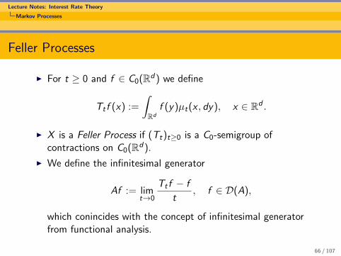
I For t ≥ 0 and f ∈ C0(Rd) we define

Tt f (x) :=

∫Rd

f (y)µt(x , dy), x ∈ Rd .

I X is a Feller Process if (Tt)t≥0 is a C0-semigroup ofcontractions on C0(Rd).

I We define the infinitesimal generator

Af := limt→0

Tt f − f

t, f ∈ D(A),

which conincides with the concept of infinitesimal generatorfrom functional analysis.

66 / 107


Markov Processes

Stochastic Differential Equations as Markov processes

I Let b : Rd → Rd and σ : Rd → Rd×m. Consider the SDE

dX xt = b(Xt)dt + σ(Xt)dWt , X x

0 = x

I We assume that the solution exists for all times and any initialvalue in some state space S as a Feller-Markov process.

I Set a := σσ>. We have C 20 (Rd) ⊂ D(A) and

Af (x) =1

2

d∑i ,j=1

aij(x)∂2

∂xi∂xjf (x)+〈b(x),∇f (x)〉, f ∈ C 2

0 (Rd).

I Example: For a Brownian motion W we have A = 12 ∆.

67 / 107


Markov Processes

Kolmogorov Backward Equation

We assume there exist transition densities p(t, x , y) such that

P(Xt ∈ B |Xs = x) =

∫B

p(t − s, x , y)dy .

I Recall that the generator is given by

Af (x) =1

2

d∑i ,j=1

aij(x)∂2

∂xi∂xjf (x) +

d∑i=1

bi (x)∂

∂xif (x).

I Kolmogorov backward equation: For fixed y ∈ Rd we have

∂

∂tp(t, x , y) = A p(t, x , y),

i.e. the equation acts on the backward (initial) variables. Italso holds in the sense of distribution for the expectationfunctional (t, x) 7→ E (f (X x

t )). 68 / 107


Markov Processes

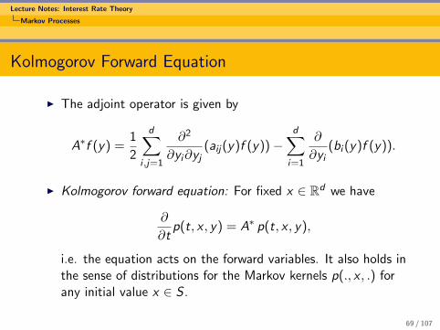
Kolmogorov Forward Equation

I The adjoint operator is given by

A∗f (y) =1

2

d∑i ,j=1

∂2

∂yi∂yj(aij(y)f (y))−

d∑i=1

∂

∂yi(bi (y)f (y)).

I Kolmogorov forward equation: For fixed x ∈ Rd we have

∂

∂tp(t, x , y) = A∗ p(t, x , y),

i.e. the equation acts on the forward variables. It also holds inthe sense of distributions for the Markov kernels p(., x , .) forany initial value x ∈ S .

69 / 107


Markov Processes

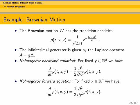
Example: Brownian Motion

I The Brownian motion W has the transition densities

p(t, x , y) =1√2πt

e−(y−x)2

2t .

I The infinitesimal generator is given by the Laplace operatorA = 1

2 ∆.I Kolmogorov backward equation: For fixed y ∈ Rd we have

d

dtp(t, x , y) =

1

2

∂2

∂x2p(t, x , y).

I Kolmogorov forward equation: For fixed x ∈ Rd we have

d

dtp(t, x , y) =

1

2

∂2

∂y 2p(t, x , y).

70 / 107


Markov Processes

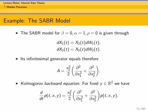
Example: The SABR Model

I The SABR model for β = 0, α = 1, ρ = 0 is given through

dX1(t) = X2(t)dW1(t),

dX2(t) = X2(t)dW2(t).

I Its infinitesimal generator equals therefore

A =x2

2

2

(∂2

∂x21

+∂2

∂x22

).

I Kolmogorov backward equation: For fixed y ∈ R2 we have

d

dtp(t, x , y) =

x22

2

(∂2

∂x21

+∂2

∂x22

)p(t, x , y).

71 / 107


Markov Processes

Example: The SABR model

I Kolmogorov forward equation: For fixed x ∈ R2 we have

d

dtp(t, x , y) =

(∂2

∂y 21

+∂2

∂y 22

)y 2

2

2p(t, x , y).

I Notice that in general the foward and backward equation aredifferent.

72 / 107


Markov Processes

Construction of finite factor models

By the choice of a finite dimensional Markov process (X 1, . . . ,X n)and the choice of an expression

Rt = H(Xt)

for the short rate, one can construct – due to the Markov property– consistent finite factor model

E (exp(−∫ T

tH(Xs)ds) = P(t,T ) = exp(−

∫ T

tG (t, r ,Xt)dr),

for all 0 ≤ t ≤ T , G satisfies a certain P(I)DE.

73 / 107


Markov Processes

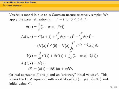
Vasicek’s model is due to is Gaussian nature relatively simple: Weapply the parametrization x = T − t for 0 ≤ t ≤ T :

Λ(x) =1

β(1− exp(−βx))

A0(t, x) = r∗(x + t) +ρ2

2Λ(x + t)2 − ρ2

2Λ(x)2−

− (Λ′(x))2r∗(0)− Λ′(x)

∫ t

0e−β(t−s)b(s)ds

b(t) =d

dtr∗(t) + βr∗(t) +

ρ2

2β(1− exp(−2βt))

A1(t, x) = Λ′(x)

dRt = (b(t)− βRt)dt + ρdWt

for real constants β and ρ and an ”arbitrary” initial value r∗. Thissolves the HJM equation with volatility σ(r , x) = ρ exp(−βx) andinitial value r∗.

74 / 107


Markov Processes

The CIR analysis is more involved:

A0(t, x) = g(t, x)− c(t)Λ′(x)

g(t, x) = r∗(t + x)+

+ρ2

∫ t

0g(t − s, 0)(ΛΛ′)(x + t − s)ds

c(t) = g(t, 0), b(t) =d

dtc(t) + βc(t)

A1(t, x) = Λ′(x)

dRt = (b(t)− βRt)dt + ρR12t dWt

for real constants β and ρ and an ”arbitrary” initial value r∗. This

solves the HJM equation with volatility σ(r , x) = ρ(ev0(r))12 Λ(x)

and initial value r∗.

75 / 107


The SABR model

I The SABR model combines an explicit expression for impliedvolatility with attractive dynamic properties for impliedvolatilities.

I In contrast to affine models stochastic volatility is a lognormalrandom variable.

I it is a beautiful piece of mathematics.

I all important details can be found in [2].

76 / 107


The SABR model

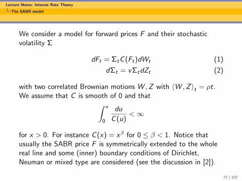
We consider a model for forward prices F and their stochasticvolatility Σ

dFt = ΣtC (Ft)dWt (1)

dΣt = vΣtdZt (2)

with two correlated Brownian motions W ,Z with 〈W ,Z 〉t = ρt.We assume that C is smooth of 0 and that∫ x

0

du

C (u)<∞

for x > 0. For instance C (x) = xβ for 0 ≤ β < 1. Notice thatusually the SABR price F is symmetrically extended to the wholereal line and some (inner) boundary conditions of Dirichlet,Neuman or mixed type are considered (see the discussion in [2]).

77 / 107


The SABR model

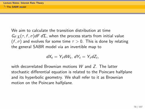
We aim to calculate the transition distribution at timeGF ,Σ(τ, f , σ)dF dΣ, when the process starts from initial value(f , σ) and evolves for some time τ > 0. This is done by relatingthe general SABR model via an invertible map to

dXt = YtdWt , dYt = YtdZt ,

with decorrelated Brownian motions W and Z . The latterstochastic differential equation is related to the Poincare halfplaneand its hyperbolic geometry. We shall refer to it as Brownianmotion on the Poincare halfplane.

78 / 107


The SABR model

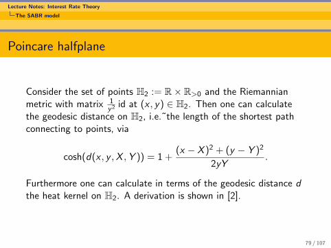
Poincare halfplane

Consider the set of points H2 := R× R>0 and the Riemannianmetric with matrix 1

y2 id at (x , y) ∈ H2. Then one can calculatethe geodesic distance on H2, i.e.˜the length of the shortest pathconnecting to points, via

cosh(d(x , y ,X ,Y )) = 1 +(x − X )2 + (y − Y )2

2yY.

Furthermore one can calculate in terms of the geodesic distance dthe heat kernel on H2. A derivation is shown in [2].

79 / 107


The SABR model

Applying the invertible map φ

(f , σ) 7→( 1√

1− ρ2(

∫ f

0

du

C (u)− ρsigma), σ)

to the equation

dFt = ΣtC (Ft)dWt , dΣt = ΣtdZt

leads to the Poincare halfplane’s Brownian motion perturbed by adrift term. From the point of view of the SABR model one has toadd a drift such that the φ−1 transformation of it is precisely theBrownian motion of the Poincare halfplane.

80 / 107


The SABR model

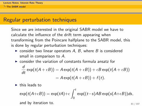
Regular perturbation techniques

Since we are interested in the original SABR model we have tocalculate the influence of the drift term appearing whentransforming from the Poincare halfplane to the SABR model, thisis done by regular perturbation techniques:

I consider two linear operators A, B, where B is consideredsmall in comparison to A.

I consider the variation of constants formula ansatz ford

dtexp(t(A + εB)) = A exp(t(A + εB)) + εB exp(t(A + εB))

= A exp(t(A + εB)) + f (t).

I this leads to

exp(t(A+εB)) = exp(tA)+ε

∫ t

0exp((t−s)AB exp(s(A+εB))ds,

and by iteration to. 81 / 107


The SABR model

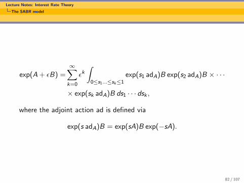
exp(A + εB) =∞∑k=0

εk∫

0≤s1...≤sk≤1exp(s1 adA)B exp(s2 adA)B × · · ·

× exp(sk adA)B ds1 · · · dsk ,

where the adjoint action ad is defined via

exp(s adA)B = exp(sA)B exp(−sA).

82 / 107


The SABR model

Local volatility

A good approximation for implied volatility is given by localvolatility, which can be calculated in many models by the followingformula

σ(t,K )2 =∂∂T C (T ,K )∂2

∂K2 C (T ,K ),

being the answer to the question which time-dependent volatilityfunction σ to choose such that dSt = σ(t, St)dWt mimicks thegiven prices C (T ,K ), i.e. for T ,K ≥ 0 it holds

C (T ,K ) = E ((ST − K )+).

83 / 107


The SABR model

The reasoning behind Dupire’s formula for local volatility is thatthe transition distribution of a local volatility model satisfiesKolmogorov’s forward equation in the forward variables

∂2

∂S2σ(t,S)2p(T ,S , s) =

∂

∂Tp(T ,S , s).

On the other hand it is well-known by Breeden-Litzenberger that

p(T ,K , s) =∂2

∂K 2C (T ,K ),

which leads after twofold integration of Kolmogorov’s forwardequation by parts to Dupire’s formula.

84 / 107


The SABR model

In terms of the transition function of the SABR model Dupire’sformula reads as

σ(T ,K )2 =C (K )2

∫Σ2G (T ,K ,Σ, f , σ)dΣ∫

G (T ,K ,Σ, f , σ)dΣ,

which can be evaluated by Laplace’s principle as shown in [2] sinceone has at hand a sufficiently well-known expression for G .

85 / 107


HJM-models

Levy driven HJM models

Let L be a d-dimensional Levy process with Levy exponent κ, i.e.

E (exp(〈u, Lt〉) = exp(κ(u)t)

for u ∈ U an open strip in Cd containing iRd , where κ is alwaysdefined. Then it is well-known that

exp(−∫ t

0κ(αs)ds +

∫ t

0〈αs , dLs〉)

is a local martingale for predictable strategies alpha such that bothintegrals are well-defined. Notice that the strategy α is Rd -valuedand that κ has to be defined on αs .

86 / 107


HJM-models

0 2 4 6 8 10

−1

01

23

45

6

t

3 trajectories of a stable process

87 / 107


HJM-models

0 2 4 6 8 10

02

46

8

t

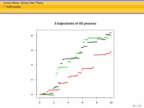
3 trajectories of VG process

88 / 107


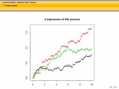
HJM-models

0 2 4 6 8 10

0.0

0.5

1.0

1.5

t

3 trajectories of NIG process

89 / 107


HJM-models

We can formulate a small generalization of the previous result byconsidering a parameter-dependence in the strategies αS . There isone Fubini argument necessary to prove the result: we assumecontinuous dependence of αS on S , then

Nut = exp(

∫ t

0

∫ T

u

d

dSκ(

∫ S

uαUs dU)ds +

∫ t

0

∫ T

u〈αS

s dS , dLs〉)

is a local martingale. Notice here that Ntt is not a local martingale,

but ∫ t

0(dNu

t )u=t

is one, since – loosely speaking – it is the sum of local martingaleincrements.

90 / 107


HJM-models

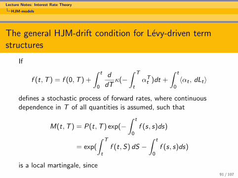
The general HJM-drift condition for Levy-driven termstructures

If

f (t,T ) = f (0,T ) +

∫ t

0

d

dTκ(−

∫ T

tαTt )dt +

∫ t

0〈αt , dLt〉

defines a stochastic process of forward rates, where continuousdependence in T of all quantities is assumed, such that

M(t,T ) = P(t,T ) exp(−∫ t

0f (s, s)ds)

= exp(

∫ T

tf (t,S) dS −

∫ t

0f (s, s)ds)

is a local martingale, since91 / 107


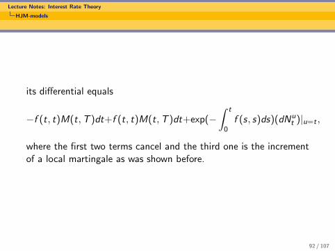
HJM-models

its differential equals

−f (t, t)M(t,T )dt+f (t, t)M(t,T )dt+exp(−∫ t

0f (s, s)ds)(dNu

t )|u=t ,

where the first two terms cancel and the third one is the incrementof a local martingale as was shown before.

92 / 107


HJM-models

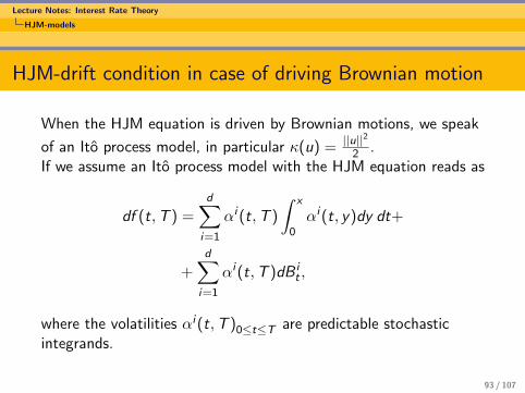
HJM-drift condition in case of driving Brownian motion

When the HJM equation is driven by Brownian motions, we speak

of an Ito process model, in particular κ(u) = ||u||22 .

If we assume an Ito process model with the HJM equation reads as

df (t,T ) =d∑

i=1

αi (t,T )

∫ x

0αi (t, y)dy dt+

+d∑

i=1

αi (t,T )dB it ,

where the volatilities αi (t,T )0≤t≤T are predictable stochasticintegrands.

93 / 107


HJM-models

Musiela parameterization

The forward rates (f (t,T ))0≤t≤T are best parametrized through

r(t, x) := f (t, t + x)

for t, x ≥ 0 (Musiela parametrization). This allows to considerspaces of forward rate curves, otherwise the domain of definition ofthe forward rate changes along running time as it equals [t,∞[.

94 / 107


HJM-models

Forward Rates as states

This equation is best analysed as stochastic evolution on a Hilbertspace H of forward curves making it thereon into a Markov process

σi (t, .) = σi (rt), σi : H → H

for some initial value r0 ∈ H. We require:I H is a separable Hilbert space of continuous functions.I point evalutations are continuous with respect to the topology

of a Hilbert space.I The shift semigroup (Str)(x) = r(t + x) is a strongly

continuous semigroup on H with generator ddx .

I The map h 7→ S(h) with S(h)(x) := h(x)∫ x

0 h(y)dy satisfies

||S(h)|| ≤ K ||h||2

for all h ∈ H with S(h) ∈ H.

95 / 107


HJM-models

An example

Let w : R≥0 → [1,∞[ be a non-decreasing C 1-function with

1

w13

∈ L1(R≥0),

then we define

||h||w := |h(0)|+∫R≥0

|h′(x)|w(x)dx

for all h ∈ L1locwith h′ ∈ L1

loc (where h′ denotes the weakderivative). We define Hw to be the space of all functions h ∈ L1

loc

with h′ ∈ L1loc such that ||h||w <∞.

96 / 107


HJM-models

Finite Factor models

Given an initial forward rate T 7→ f (0,T ) or T 7→ P(0,T ),respectively. A finite factor model at initial value r∗ is a mapping

G : 0 ≤ t ≤ T × Rn ⊂ R2≥0 × Rn → R

together with an Markov process (Xt)t≥0 such that

f (t,T ) = G (t,T ,X 1t , ...,X

nt )

for 0 ≤ t ≤ T and T ≥ 0 is an arbitrage-free evolution of forwardrates. The process (Xt)t≥0 is called factor process, its dimension nis the dimension of the factor model.

97 / 107


HJM-models

In many cases the map G is chosen to have a particularly simplestructure

G (t,T , z1, ..., zn) = A0(t,T ) +n∑

i=1

Ai (t,T )z i .

In these cases we speak of affine term structure models, the factorprocesses are also affine processes. Remark that G must reproducethe initial value

G (0,T , z10 , ..., z

n0 ) =: r∗(T )

for T ≥ 0. The famous short rate models appear as 1- or2-dimensional cases (n = 1, 2 – time is counted as additionalfactor).

98 / 107


HJM-models

The consistency problem

It is an interesting and far reaching question if – for a givenfunction G (t,T , z) – there is a Markov process such that theyconstitute a finite factor model together.

99 / 107


HJM-models

Svensson family

An interesting example for a map G is given by the Svensson family

G (t,T , z1, . . . , z6) = z1 + z2 exp(−z3(T − t))+

+ (z4 + z5(T − t)) exp(−z6(T − t)),

since it is often applied by national banks. The wishful thought tofind an underlying Ito-Markov process such that G is consistentwith an arbitrage free evolution of interest rates is realized by aone factor Gaussian process.

100 / 107


References

[1] Damir Filipovic.Term structure models: A Graduate Course.see http://sfi.epfl.ch/op/edit/page-12795.html

[2] Patrick Hagan, Andrew Lesniewski, and Diana Woodward.Probability Distribution in the SABR Model of StochasticVolatility.see http://lesniewski.us/working.html

[3] Martin Keller-Ressel, Antonis Papapantoleon, JosefTeichmann.A new approach to LIBOR modeling.see http://www.math.ethz.ch/~jteichma/index.php?

content=publications

101 / 107

http://sfi.epfl.ch/op/edit/page-12795.html

http://lesniewski.us/working.html

http://www.math.ethz.ch/~jteichma/index.php?content=publications

http://www.math.ethz.ch/~jteichma/index.php?content=publications



[4] Damir Filipovic, Stefan Tappe.Existence of Levy term structure models.seehttp://www.math.ethz.ch/~tappes/publications.php

102 / 107

http://www.math.ethz.ch/~tappes/publications.php




I What are ZCBs, yield curves, forward curves, short rates,caplets, floorlets, swaps, swap rates, roll-over-portfolios?

I What is a LIBOR rate (simple forward rate) on nominal onereceived at terminal date and what is its fair value before?Some relations of cap, floors, swaptions like in exercise 2 ofSheet 2.

I Black’s formula for caps and floors – derivation andassumptions?

I Black’s formula for swaptions – derivation and assumptions?

103 / 107




I Change of numeraire theorem: exercise 1,2 of Sheet 7.

I What is the LIBOR market model (Exercise 3 of Sheet 7)?

I What is the foward measure model (Exercise 2 of Sheet 8).

I What is an affine LIBOR model and what are its maincharacteristics (Axiom 1 – 3 can be satisfied)?

I What is the Fourier method of derivative pricing (Exercise 1 ofSheet 9)?

104 / 107




I Levy processes and their cumulant generating function(Exercise 1 of Sheet 11).

I What is the HJM-drift condition for Brownian motion andwhich Hilbert spaces of forward rates can be considered?

I Derivation of the HJM-drift condition for Levy driven interestrate models.

I Why are models for the whole term structure attractive?What lie their difficulties?

105 / 107




I What is the general SABR model and how is it related to thePoincare halfplane?

I What is the geodesic distance in the Poincare halfplane(definition) and how can we calculate it (eikonal equation),Exercise 5 on Sheet 9? What is the natural stochastic processon the Poincare halfplane – can we calculate its heat kernel?

I What is local volatility and how can we calculate it (Dupire’sformula)?

I Implied volatility in interest rate markets: which tractabilitydo we need from models and what do market models, forwardmeasure models, affine models, the SABR model, HJMmodels provide?

106 / 107




I Short rate models: the Vasicek model (Exercise 1 of Sheet 4).

I Short rate models: the CIR model (Exericse 2 of Sheet 4, notevery detail).

I Short rate models: Hull-White extension of the Vasicek model(Exercise 2 of Sheet 6).

I Is short rate easy to model from an econometric point of view?

107 / 107

lecture notes: interest rate theory - eth zjteichma/lecture_notes_ir... · · 2011-01-03lecture...

Documents