Lecture Notes on Monte Carlo Methods

Andrew Larkoski

November 7, 2016

1 Lecture 1

This week we deviate from the text and discuss the important topic of Monte Carlo methods.Monte Carlos are named after the famous casino in Monaco, where chance and probabilityrule. This week we will discuss how to numerically simulate outcomes of an experiment(“data”). This is a huge and important subject into which we will just dip our feet.

Every experiment in physics corresponds to sampling a probability distribution for thequantity that you measure.

Example 1: What is the distribution of the times between cars passing a point on the road?

We must measure the time it takes for another car to pass the point. As moreand more cars are measured, we have more and more data points on which todetermine the distribution. We will refer to each instance or data point of anexperiment as an event. Any experiment performed by humans contains only afinite number of events. How can we model this?

t = 0 t = 5s t = 12st = 15s

t = 25s“event 1”

car 1 car 2 car 3 car 4

Figure 1: Illustration of four events in the measurement of the distribution in time of carspassing a point.

Example 2: What is the distribution of the positions of a particle in an infinite square well?

We must prepare n identical infinite square well systems and measure the positionof the particle in each system. Each measurement of the position is an event.Note that to determine the distribution requires repeatability: the measurements

1

x = 0.3 x = 0.6 x = 0.04

event 1 event 2

event 3

0

1

· · ·

Figure 2: Illustration of an example of three events in which the position of the particle inthe infinite square well was measured.

must be done on identical systems. Otherwise, we do not know how to interpretour results. (The possibility of repeatability is intimately related to energy andmomentum conservation, but that’s a topic for another class.) How do we samplea probability distribution numerous times?

For any finite number of measurements, we cannot reproduce the probability distributionexactly, but we can approximate it arbitrarily precisely. To do this, take our set of events:

I = {events of experiment} , (1)

and divide them into sets according to their values; these are called bins. For example,for the infinite square well on the domain x 2 [0, 1], we will divide the possible measuredpositions into N

bins

bins. If an event has a measured position

x 2i � 1

N

bins

,

i

N

bins

�, (2)

for an integer i 2 [1, Nbins

], then we add 1 to this bin.Doing this for all of the N

ev

events in an experiment generates a histogram, which is afinite approximation to a smooth distribution. This will produce a histogram whose entriessum to the total number of events. If instead we want a histogram that integrates to 1, sothat it can be directly interpreted as a probability distribution, instead of adding 1 to theith bin we add

1

�x

i

N

ev

. (3)

To see that this results in a histogram that integrates to 1, we will denote the number ofevents in the ith bin by N

i

. Then the integral of the histogram is just the sum:

N

binsX

i=1

�x

i

· N

i

�x

i

N

ev

=1

N

ev

N

binsX

i=1

N

i

= 1 . (4)

2

To do this integral, we have used that the integration measure dx = �x

i

and that the sumof the events in each bin is just the total number of events.

To interpret and compare our data to a prediction, we want to generate a histogram ofevents numerically. That is, we want to generate pseudodata, which are a finite numberof events drawn from a given probability distribution of our choice. We can then comparedirectly between the histogram of our real data to our pseudodata, and attempt to drawconclusions. There are numerous methods to quantitatively judge the goodness-of-fit of ahistogram by a probability distribution (things like the Kolmogorov-Smirnov test, Student’st-test,1 etc.), but we won’t discuss them here.

While this procedure sounds relatively simple, there are many challenges that must beovercome to produce pseudodata:

• To sample a probability distribution requires the generation of random numbers. Wewill typically work with uniform, real random numbers on the domain of [0, 1]. Wewill show that this is su�cient to sample an arbitrary probabiltiy distribution. How isthis accomplished? How does Mathematica generate random real numbers?

– Well, Mathematica actually doesn’t produce truly random numbers. The numbersgenerated by Mathematica (or any other programming language) is pseudoran-dom: they appear random, but are actually defined by a deterministic algorithm.Good pseudorandom number generators repeat on scales of 210000 calls; this iscalled the period of the generator. This will be su�cient, though later in thisclass we will discuss other choices. One of the most common pseudorandom num-ber generator is the “Mersenne Twister”, which has a period equal to a Mersenneprime (see the poster outside Joel’s o�ce).

– There are some examples of truly random numbers and random number genera-tors. The most famous is probably the collection in the book “A Million RandomDigits with 100,000 Normal Deviates”. This book is copyrighted, and if you arein need of amusement, check out the Amazon reviews for this book. Now, thereare companies producing true random number generators which exploit the ran-domness of quantum noise, though they aren’t found in every household yet.

• More than likely, however, you actually don’t know the probability distribution thatyou should be sampling. For the infinite square well example, we know the probabilitydistribution and can sample it e�ciently. What do you do if you don’t know it? Forexample, what if you want to determine the distribution of spins of a material in 2Dat finite temperature? How do you make pseudodata of an event (a measurement ofthe spins in the system)?

– We do know what the configuration of spins should satisfy physically. Energyis minimized if the spins align, and so we can check spin by spin if they are

1Student was the pseudonym of William Sealy Gosset, who worked for the Guinness brewery. Gosset

applied statistics to quality control of the beer produced at Guinness but was forbidden to publish, so he

created the name “Student” to evade the restriction.

3

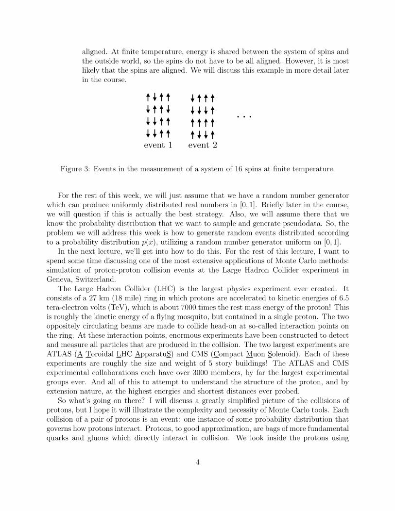
aligned. At finite temperature, energy is shared between the system of spins andthe outside world, so the spins do not have to be all aligned. However, it is mostlikely that the spins are aligned. We will discuss this example in more detail laterin the course.

· · ·

event 1 event 2

Figure 3: Events in the measurement of a system of 16 spins at finite temperature.

For the rest of this week, we will just assume that we have a random number generatorwhich can produce uniformly distributed real numbers in [0, 1]. Briefly later in the course,we will question if this is actually the best strategy. Also, we will assume there that weknow the probability distribution that we want to sample and generate pseudodata. So, theproblem we will address this week is how to generate random events distributed accordingto a probability distribution p(x), utilizing a random number generator uniform on [0, 1].

In the next lecture, we’ll get into how to do this. For the rest of this lecture, I want tospend some time discussing one of the most extensive applications of Monte Carlo methods:simulation of proton-proton collision events at the Large Hadron Collider experiment inGeneva, Switzerland.

The Large Hadron Collider (LHC) is the largest physics experiment ever created. Itconsists of a 27 km (18 mile) ring in which protons are accelerated to kinetic energies of 6.5tera-electron volts (TeV), which is about 7000 times the rest mass energy of the proton! Thisis roughly the kinetic energy of a flying mosquito, but contained in a single proton. The twooppositely circulating beams are made to collide head-on at so-called interaction points onthe ring. At these interaction points, enormous experiments have been constructed to detectand measure all particles that are produced in the collision. The two largest experiments areATLAS (A Toroidal LHC ApparatuS) and CMS (Compact Muon Solenoid). Each of theseexperiments are roughly the size and weight of 5 story buildings! The ATLAS and CMSexperimental collaborations each have over 3000 members, by far the largest experimentalgroups ever. And all of this to attempt to understand the structure of the proton, and byextension nature, at the highest energies and shortest distances ever probed.

So what’s going on there? I will discuss a greatly simplified picture of the collisions ofprotons, but I hope it will illustrate the complexity and necessity of Monte Carlo tools. Eachcollision of a pair of protons is an event: one instance of some probability distribution thatgoverns how protons interact. Protons, to good approximation, are bags of more fundamentalquarks and gluons which directly interact in collision. We look inside the protons using

4

Figure 4: A view of Geneva, Switzerland, from the Jura Mountain range to the west. Thecity of Geneva is located at the end of Lake Geneva, the ring of the Large Hadron Collideris illustrated in yellow, the runway of the Geneva airport is visible as a size reference, andMont Blanc is present o↵ in the distance. Photo Credit: CERN.

the “Neanderthal method”: we smash things together and determine what was inside bywhat comes out (cf. to opening presents on your birthday). A huge number of particlesare produced in these collisions; things called pions, kaons, muons, and familiar protons,photons, and electrons. Schematically, we might illustrate one such event as in figure 6.

Arrows pointing toward the center represent the colliding protons while arrows pointingaway represent the particles that are produced. I have just illustrated one of a nearlyinfinite number of possible collections of produced particles (called “final states”). Also,these particles can have any relativistic momentum, only subject to momentum conservation.Additionally, it is the ATLAS and CMS experiments that measure properties of the finalstate particles (like their charge, energy, etc.). They do not have little labels on them. Anyexperiment is imperfect: energies are not measured arbitrarily accurately; angles are smearedby finite resolution; there are cables that are in the way of equipment; etc. With all of thesechallenges, how are we able to make predictions for the final state of LHC collisions?

This problem is nearly ideal for a Monte Carlo solution for the following reasons:

1. In proton-proton collisions, there are essentially an infinite number of possible out-comes. While there is a fundamental theory underlying proton collision physics (theStandard Model), it is amazingly complex and there is no known way (and perhaps

5

Figure 5: An image of the ATLAS experiment during its construction. Notice the human forscale; the large piping located around the experiment houses currents that source toroidalelectromagnets. Photo Credit: CERN.

no way whatsoever) to achieve exact, analytic solutions for probability distributions.By incorporating the physics of the Standard Model, we are able to construct MonteCarlo simulations that produce final states faithfully according to their probability tooccur.

2. Monte Carlo also enables for realistic outcomes to be simulated. We not only needthe types of particles produced in the final state, but also their momentum, which isa series of four real numbers. This is essentially impossible with a large number ofparticles in the final state. However, to good approximation, we are able to assumethat the production of particles is a Markov process: that is, the production probabilityof additional particles only depends on what particles currently exist. This enables asimple recursive, iterative algorithm to be able to generate arbitrary final states.

3. Detectors and experiments are imperfect, so we also need to model the response of theequipment to particular particles with certain momentum to make realistic pseudo-data. Because the Monte Carlo produces individual pseudoevents, it is straightforwardto “measure” the final state with a detector simulation. The results of the pseudoex-periments can then be compared to real data to test hypotheses or to discover newparticles and forces of nature!

The most widely used Markov Chain Monte Carlo simulators go by names like “Pythia”and “Herwig” and are used ubiquitously to understand the data from ATLAS and CMS.

6

e�e+

p+

n

� �0�+

p+

�0

p+

Figure 6: Schematic representation of a proton-proton collision event. Note charge conser-vation.

2 Lecture 2

Last lecture, we introduced the idea of Monte Carlo methods and the need for simulationof pseudodata. This becomes important for modeling e↵ects of finite data samples, finiteexperimental resolution, or for understanding systems for which the analytic probabilitydistribution is unknown or even unknowable. In this lecture, we discuss in detail the math-ematical foundation for Monte Carlo methods.

With the basis from previous lecture, we assume that we have a (known) probabilitydistribution p(x) and can e�ciently sample (pseudo)random real numbers on [0, 1]. How dowe generate a set of numbers {x} distributed according to p(x)?

For simplicity, let’s assume that p(x) is defined on x 2 [0, 1] so that

Z1

0

dx p(x) = 1 . (5)

The results that follow are true for arbitrary probability distributions; just confining ourselvesto x 2 [0, 1] is for compactness. The probability for a value to lie within dx of x is p(x) dx.Assuming the inverse exists, we can make the change of variables to y as:

p(x) dx = p(x(y))dx

dy

dy , (6)

where x(y) is the change of variables. This then defines a new probability distribution:

p̄(y) = p(x(y))dx

dy

. (7)

Now, if we assume that this change of variables renders p̄(y) uniform on y 2 [0, 1], then

p(x(y)) =dy

dx

) y =

Zx

0

dx

0p(x0) + c . (8)

7

c is an integration constant which is 0 because p(x) is normalized.The integral Z

x

0

dx

0p(x0) (9)

is just the cumulative distribution, or the probability that the random variable is less thanx. We will denote it by

⌃(x) =

Zx

0

dx

0p(x0) . (10)

Note that ⌃(0) = 1, ⌃(1) = 1, and ⌃(x) is monotonic on x 2 [0, 1]. Because it is monotonic,⌃(x) can always be inverted. Now, we can solve for x:

x = ⌃�1(y) . (11)

That is, the random variable x distributed as p(x) can be generated by inverting the cumu-lative distribution and using the uniformly distributed y 2 [0, 1] as the independent variable.

The fundamental step for this method of sampling a distribution is generating randomnumbers distributed on [0, 1]. The following Mathematica function rand outputs an arrayof random numbers distributed on [0, 1] using its internal random number generator:

rand[Nev ]:=Module[{randtab,r},randtab={};For[i = 1, i Nev, i++,

r = RandomReal[{0,1}];AppendTo[randtab,r];

];

Return[randtab];

];

This is the central result for Monte Carlo simulation. “Any” (invertible, closed form)probability distribution can be sampled from a uniform distribution. Let’s see how thisworks in a couple of examples.

Example.

Let’s consider a quantum particle in the infinite square well. The probabilitydistribution for a the position of a particle in the ground state of a square wellon x 2 [0, 1] is

p(x) = 2 sin2(⇡x) . (12)

Note that this is normalized. The cumulative distribution is

⌃(x) =

Zx

0

dx

0p(x0) = x � sin(2⇡x)

2⇡. (13)

8

Then, to sample this distribution, we set the cumulative distribution equal to y,which is uniformly distributed on [0, 1]:

y = x � sin(2⇡x)

2⇡. (14)

This isn’t solvable for x in closed form, but for a given y 2 [0, 1], there exists aunique value of x that can be determined numerically (using Newton’s method,for example, to find roots).

Example.

Let’s consider the probability distribution of the time it takes a radioactive el-ement to decay. Radioactive decay of an atom is governed by its half-life, �.At time t = �, there is a 50% chance that the atom has decayed. Equivalently,given a sample of material composed of an unstable element, 50% of it will havedecayed by t = �. The probability distribution of the time t it takes one of theseunstable atoms to decay is

p(t) =log 2

�

e

� t� log 2

, (15)

where the time t 2 [0,1). That is, the atom can decay any time after we startwatching (at time t = 0). Note that the ratio of the probability at time t = � tot = 0 is 1/2:

p(t = �)

p(t = 0)= e

� log 2 =1

2. (16)

That is, the likelihood that the atom is still there at time t = � is 50%.

Now, we would like to be able to sample this distribution via a Monte Carlo. So,we first determine the cumulative distribution:

⌃(t) =

Zt

0

dt

0p(t0) = 1 � e

� t� log 2

, (17)

which is 0 at t = 0 and 1 at t = 1, and is monotonic. Next, we set this equal toa uniformly distributed y 2 [0, 1] and invert, solving for t. We find

t = � �

log 2log(1 � y) . (18)

Note that for y 2 [0, 1], this time ranges over t 2 [0,1).

The following Mathematica function expdist samples an exponential distribu-tion with half-life � and outputs a histogram of the resulting distribution. Itsarguments are �, the number of events Nev, the end-point of the histogrammaxpoint, and the number of bins in the histogram Nbins:

9

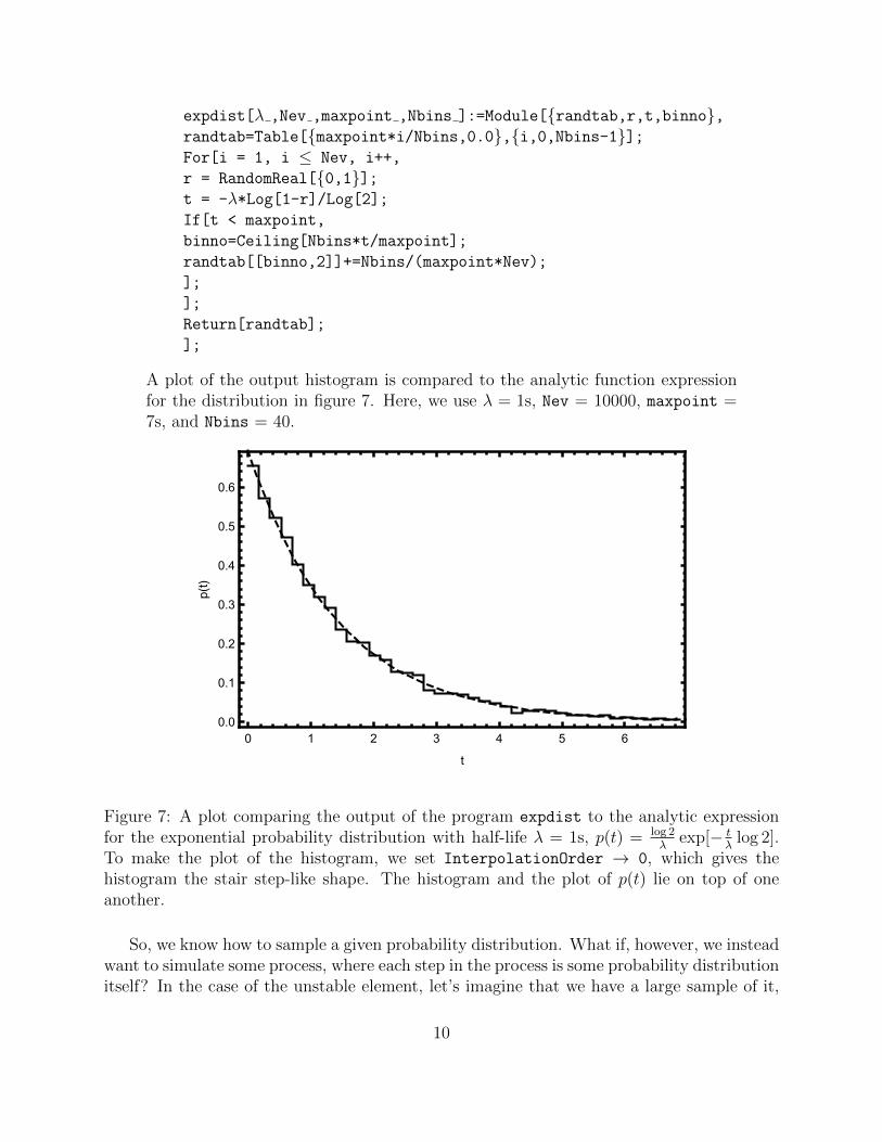
expdist[� ,Nev ,maxpoint ,Nbins ]:=Module[{randtab,r,t,binno},randtab=Table[{maxpoint*i/Nbins,0.0},{i,0,Nbins-1}];For[i = 1, i Nev, i++,

r = RandomReal[{0,1}];t = -�*Log[1-r]/Log[2];

If[t < maxpoint,

binno=Ceiling[Nbins*t/maxpoint];

randtab[[binno,2]]+=Nbins/(maxpoint*Nev);

];

];

Return[randtab];

];

A plot of the output histogram is compared to the analytic function expressionfor the distribution in figure 7. Here, we use � = 1s, Nev = 10000, maxpoint =7s, and Nbins = 40.

0 1 2 3 4 5 60.0

0.1

0.2

0.3

0.4

0.5

0.6

t

p(t)

Figure 7: A plot comparing the output of the program expdist to the analytic expressionfor the exponential probability distribution with half-life � = 1s, p(t) = log 2

�

exp[� t

�

log 2].To make the plot of the histogram, we set InterpolationOrder ! 0, which gives thehistogram the stair step-like shape. The histogram and the plot of p(t) lie on top of oneanother.

So, we know how to sample a given probability distribution. What if, however, we insteadwant to simulate some process, where each step in the process is some probability distributionitself? In the case of the unstable element, let’s imagine that we have a large sample of it,

10

and we want to determine the number of atoms that decay in a given time interval t 2 [0, T ].How do we do this? For this problem and many others in physics, it can be expressed as aMarkov Chain, which we will explore now.

To a good approximation, radioactive decays in a sub-critical sample are independent ofone another. So, the probability of any atom decaying is just the exponential distribution.The exponential distribution is also “memoryless”: it is independent of when you start theclock (and appropriately normalize).2 So, to determine how many atoms decay in a time T ,we have the simple procedure:

1. Determine the time that the first atom decayed t

1

from

t

1

= � �

log 2log(1 � y) , (19)

for y uniform on [0, 1]. If t1

> T , then stop; no atoms decayed in time T . If t1

< T ,then continue.

2. Determine the time (from t = 0) that the second atom decayed t

2

from

t

2

� t

1

= � �

log 2log(1 � y) , (20)

again with y uniform on [0, 1]. If t2

> T , then stop; 1 atom decayed in time T . Ift

2

< T , then continue.

3. Determine t

3

, t

4

, . . . , and continue until tn

> T . Then, n � 1 atoms decayed.

This procedure required a couple of things to work as simply as it did. First, at every stepthe probability distribution that we sampled was identical (just the exponential distribution).Also, the time of the next decay only depended on the time of the immediate previous decay(and not on all previous decays).

Such an iterative procedure that samples a distribution recursively and each step onlydepends on the immediate previous step is a Markov Chain. What we constructed abovewould properly be called a Markov Chain Monte Carlo (MCMC). Oh, by the way, this wasreally overkill for this problem. The distribution for the number of decays in time T is justthe Poisson distribution.

Okay, we have a nice theory for how to sample a 1D probability distribution. How dowe do this for higher dimensional distributions? Let’s consider 2D for concreteness; themethod we develop there will easily generalize. Let’s consider a 2D probability distributionp(x, y) for (x, y) 2 [0, 1]. To do a similar thing as in 1D, we need to calculate the cumulativedistribution and then invert. The cumulative distribution is

⌃(x, y) =

Zx

0

dx

0Z

y

0

dy

0p(x0

, y

0) , (21)

2We’re simplifying things here a bit to describe the method. We’re making the somewhat silly assumption

that the atoms decay 1 at a time.

11

but it is not clear at all how to invert this. How do you uniquely invert a function of twovariables into two other variables? To proceed, we need another tactic.

Instead, if we are able to express p(x, y) as the product of two 1D probability distributions,then we can apply our methods from 1D to 2D distributions. We might think that we couldwrite

p(x, y) = p(x)p(y) , (22)

but this is not true in general. Instead, we utilize the definition of a conditional probability:

p(x|y) = p(x, y)

p(y), (23)

where we define

p(y) =

Z1

0

dx p(x, y) . (24)

We read p(x|y) as “probability of x given y”, and the conditional probability is a 1D proba-bility distribution itself. For p(x|y), y is a fixed parameter, and not a random variable. Toverify that it is normalized we have:

Z1

0

dx p(x|y) =Z

1

0

dx

p(x, y)

p(y)=

1

p(y)

Z1

0

dx p(x, y) = 1 . (25)

Using the conditional probability, we can then express a 2D distribution as a product of two1D distributions:

p(x, y) = p(y)p(x|y) = p(x)p(y|x) . (26)

Note that this representation is symmetric in x and y.Then, to sample the 2D distribution p(x, y), we first choose a random y according to p(y)

and a Monte Carlo for it. Then, given that value of y, we choose x according to p(x|y). Thisproduces a pair (x, y) chosen according to p(x, y), and we can repeat to generate a largesample of pseudodata. Let’s see how this works in an example.

12

Example.

Let’s consider the 2D distribution

p(x, y) = x+ y , (27)

where (x, y) 2 [0, 1]. Note that this is normalized:

Z1

0

dx

Z1

0

dy (x+ y) = 1 , (28)

and that the probability cannot be split up into a product: p(x, y) 6= p(x)p(y).To sample this distribution via a Monte Carlo, we therefore must first find con-ditional probabilities. Let’s find p(y). We have

p(y) =

Z1

0

dx (x+ y) = y +1

2. (29)

Then, the probability of x given y is

p(x|y) = p(x, y)

p(y)=

x+ y

y + 1

2

. (30)

So, we break up the 2D distribution as

p(x, y) = x+ y =

✓y +

1

2

◆✓x+ y

y + 1

2

◆. (31)

To then Monte Carlo this problem, we need to find the corresponding 1D cumu-lative distributions:

⌃(y) =

Zy

0

dy

0✓y

0 +1

2

◆=

y(1 + y)

2. (32)

⌃(x|y) =Z

x

0

dx

0✓x+ y

y + 1

2

◆=

x(2y + x)

2y + 1. (33)

Let’s then generate two random numbers r

1

, r

2

uniform on [0, 1], and set theseequal to the cumulative distributions and invert. That is,

⌃(y) = r

1

) y = �1

2+

r1

4+ 2r

1

, (34)

⌃(x|y) = r

2

) x = �y +p

y

2 + (2y + 1)r2

. (35)

A Mathematica program xygen that generates pairs of random numbers (x, y)distributed according to p(x, y) = x + y is provided below. The argument ofxygen is the number of events that you want to generate.

13

xygen[Nev ]:=Module[{outtab,r1,r2,x,y},outtab={};For[i = 1, i Nev, i++,

r1 = RandomReal[{0,1}];r2 = RandomReal[{0,1}];y = -1/2 +

p1/4 + 2*r1;

x = -y +py*y + (2*y+1)*r2;

AppendTo[outtab,{x,y}];];

Return[outtab];

];

3 Lecture 3

Last lecture, we developed the mathematical foundation for Monte Carlos, Markov Chainsand their utility, and how to sample multi-dimensional distributions. Everything developedlast lecture, however, required analytic calculations to invert cumulative probability distri-butions. At the very least, e�cient numerical methods were required to invert cumulativeprobability distributions. In this lecture, we will discuss how to relax this assumption ande�ciently sample generic distributions.

Let’s just assume that the probability distribution p(x) exists on the domain x 2 [0, 1] andwe want to sample it. It might not even have an analytic expression, but just be expressedas a collection of points. For this general case, there’s no way to invert p(x) as we did before,so we need another technique. What we will do is bound the probability distribution p(x)that we want by an integrable, normalizable function q(x) that we can sample e�ciently andsimply. If we find a q(x) such that

q(x) � p(x) , (36)

for all x 2 [0, 1], then we can use the probability distribution derived from q(x) to samplep(x). Let’s see how this works.

To be concrete, let’s take q(x) constant on x 2 [0, 1]. With the maximum value of p(x)

p

max

= maxx

p(x) < 1 , (37)

we can set q(x) = p

max

so that q(x) � p(x) for all x 2 [0, 1]. We can turn q(x) into aprobability distribution by normalizing; we will call this probability distribution q̃(x):

q̃(x) = 1 . (38)

Note then thatp

max

· q̃(x) � p(x) . (39)

Because we are able to easily generate uniform random numbers on x 2 [0, 1], we are ableto generate a function that bounds p(x) everywhere. So, how to we sample p(x)? We can

14

generate additional uniform random numbers to veto those points that are inconsistent withp(x). This introduces a loss of e�ciency, but we will discuss later how to improve this.

The procedure for sampling p(x) given the bounding function q(x) = p

max

is the following:

1. Choose a random number uniformly on x 2 [0, 1].

2. Determine the maximum value of p(x) on x 2 [0, 1]; call it pmax

.

3. At the chosen random x, keep the event with probability

p

keep

=p(x)

p

max

2 [0, 1] . (40)

This can be accomplished by choosing another uniform random number y 2 [0, 1] andvetoing (=removing) the event if

y >

p(x)

p

max

. (41)

4. The events that remain will be distributed according to p(x). To normalize the distri-bution to integrate to 1, we multiply by p

max

.

Let’s see how this works in an example.

Example.

Consider again the probability distribution of the position of the particle in theground state of the infinite square well:

p(x) = 2 sin2(⇡x) (42)

for x 2 [0, 1]. Note that the maximum value of p(x) is pmax

= 2. So, we find x

by choosing a random number on [0, 1] and then keep that x with probability

p

keep

=p(x)

p

max

= sin2(⇡x) 2 [0, 1] . (43)

This never required inverting cumulative probability distributions.

A Mathematica function vetowell that implements this veto method for sam-pling probability distributions is as follows. vetowell has two arguments: thenumber of events to generate Nev, and the number of bins to put in the histogramNbins.

15

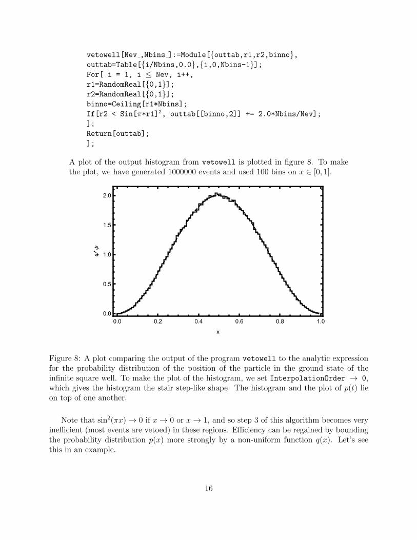
vetowell[Nev ,Nbins ]:=Module[{outtab,r1,r2,binno},outtab=Table[{i/Nbins,0.0},{i,0,Nbins-1}];For[ i = 1, i Nev, i++,

r1=RandomReal[{0,1}];r2=RandomReal[{0,1}];binno=Ceiling[r1*Nbins];

If[r2 < Sin[⇡*r1]2, outtab[[binno,2]] += 2.0*Nbins/Nev];

];

Return[outtab];

];

A plot of the output histogram from vetowell is plotted in figure 8. To makethe plot, we have generated 1000000 events and used 100 bins on x 2 [0, 1].

0.0 0.2 0.4 0.6 0.8 1.00.0

0.5

1.0

1.5

2.0

x

ψ* ψ

Figure 8: A plot comparing the output of the program vetowell to the analytic expressionfor the probability distribution of the position of the particle in the ground state of theinfinite square well. To make the plot of the histogram, we set InterpolationOrder ! 0,which gives the histogram the stair step-like shape. The histogram and the plot of p(t) lieon top of one another.

Note that sin2(⇡x) ! 0 if x ! 0 or x ! 1, and so step 3 of this algorithm becomes veryine�cient (most events are vetoed) in these regions. E�ciency can be regained by boundingthe probability distribution p(x) more strongly by a non-uniform function q(x). Let’s seethis in an example.

16

Example.

Again, let’s consider the ground state of the infinite square well, where

p(x) = 2 sin2(⇡x) . (44)

Now, consider the functionq(x) = x(1 � x) , (45)

on x 2 [0, 1]. Note that with p

max

= 2 and q

max

= 1/4, we have

8q(x) � p(x) , (46)

for all x 2 [0, 1]. The probability distribution corresponding to the function q(x)is

q̃(x) = 6x(1 � x) . (47)

Then, given Eq. 46, we can generate events according to the probability distri-bution q̃(x) and then veto appropriately. The cumulative distribution of q̃(x)is

⌃q(x) = 3x2 � 2x3

. (48)

By inverting this cumulative distribution, we can sample q̃(x) via Monte Carlo.Then, given some x from the q̃(x) distribution, we keep that event with proba-bility equal to

p

keep

=p(x)

8q(x)=

sin2(⇡x)

4x(1 � x)2 [0, 1] . (49)

The events that remain after this veto step are distributed according to p(x). Toproperly normalize the distribution, at the end we must multiply by p

max

anddivide the histogram entries by the maximum value of q̃(x).

A very reasonable question to ask, both for these pseudodata applications as well as forevaluating integrals, is what the accuracy of Monte Carlo is. To be concrete, we will justanswer the following question: what is the uncertainty on the probability to be near x, asthe number of Monte Carlo events N ! 1? That is, we want to study the Monte Carloapproximation to

P = p(x) dx . (50)

In Monte Carlo, this is approximated by the ratio of the number of events in the bin nearthe point x, N

x

, divided by the total number of events in the distribution, N . By the law oflarge numbers, this converges to P as N ! 1:

limN!1

N

x

= PN . (51)

What is the variance of this? By our Monte Carlo, all events in the bin are independentof one another and each contributes 1 to the bin. The rate at which any event populates thisbin is fixed and equal to P . These criteria uniquely define the Poisson distribution for thenumber of events in the bin. This is actually straightforward to derive, which we will do now.

17

Derivation of Poisson Distribution

We want to determine the probability distribution for the number of events in abin of a histogram that was filled via a Monte Carlo. The probability distributionthat we are sampling is p(x) and the probability P for an event to be in the binnear x is

P = p(x) dx . (52)

The probability for an event to not be in the bin is then 1 � P . All events inour pseudodata sample are independent. We therefore determine the probabilitythat there are k events in the bin near x is:

p

k

= P

k(1 � P )N�k

✓N

k

◆. (53)

This probability is called the binomial distribution for the following reason. Thefactor on the right, ✓

N

k

◆=

N !

k!(N � k)!, (54)

is read as “N choose k” and is the number of ways to pick k objects out of a setof N total objects. The probability in Eq. 53 is called the binomial distributionbecause the sum over all k corresponds to the binomial expansion:

NX

k=0

p

k

=NX

k=0

P

k(1 � P )N�k

✓N

k

◆= (P + (1 � P ))N = 1 . (55)

Now, we could stop here, but we can simplify the probability by making a fewmore assumptions. We will assume that the width of the bin is very small sothat P ⌧ 1 and k ⌧ N . In this limit, note that

✓N

k

◆=

N !

k!(N � k)!' N

k

k!, (56)

and (1 � P )k ' 1, for finite k. With these simplifications, the probability for kevents in a bin becomes

p

k

! (NP )k

k!

✓1 � NP

N

◆N

=(NP )k

k!e

�NP

, (57)

where the equality holds in the N ! 1 limit. This probability distribution iscalled the Poisson distribution. Note that it is normalized:

1X

k=0

(NP )k

k!e

�NP = 1 , (58)

has mean hki = NP and variance �

2 = hk2i � hki2 = NP .

18

Therefore, with N events in a sample and probability P for any of those events to bein a particular bin, the average number of events in the bin is NP and the variance is alsoNP . Therefore, the standard deviation (the square-root of the variance) on the number ofevents in the bin scales like

pN . The relative error is defined by the ratio of the standard

deviation to the mean. This scales like 1/pN , and so for N events, we expect an error that

scales like 1/pN . Note that this is independent of bin size and the number of dimensions

in which the probability is defined. Monte Carlo and related methods are among the moste�cient way to sample high dimensional distributions.

Later in the class, we will discuss ways to even improve this 1/pN relative error by

changing the way that random numbers are generated.Finally, I want to discuss Monte Carlo generation of non-integrable distributions. Such

distributions are not probability distributions as they cannot be normalized. For example,the function

f(x) =1

x

, (59)

on x 2 [0, 1] has undefined (infinite) integral. Such infinite distributions are unphysical; nomeasurement would ever yield 1. However, depending on assumptions and your predictiveability, one might find infinite distributions in intermediate steps of a calculation.

For example, one might attempt to calculate in degenerate perturbation theory of quan-tum mechanics and find at order n in perturbation theory:

f

n

(x) =(�1)n

x

log2n x

n!. (60)

The full distribution is a sum over n:

1X

n=0

f

n

(x) =e

� log

2

x

x

, (61)

which is finite and well-defined.There are two simple ways to sample non-integrable distributions. The first is to just

artificially cut o↵ the domain. For example, for 1/x, just stop at ✏ > 0:

f(x) =1

x

, (62)

for x 2 [✏, 1], which is normalizable. One can then do any of the techniques that we developed.Another way is to throw out the data/event interpretation of the Monte Carlo. For 1/x,

we can generate a uniform random variable x 2 [0, 1]. Then, we can fill the bin near x

by an amount equal (or proportional to) 1/x. This will then reproduce the f(x) = 1/xdistribution, but because each event does not contribute just 1 to the distribution, we can’teasily give it a probabilistic data interpretation.

This is but a tiny introduction to Monte Carlo methods.

19