lecture notes on quantum phase transitionslandsman/qpt.pdf · quantum phase transitions draft: june...
TRANSCRIPT

Lecture Notes on
Quantum Phase Transitions
Draft: June 26, 2012
N.P. Landsman
Institute for Mathematics, Astrophysics, and Particle PhysicsRadboud University Nijmegen
Heyendaalseweg 1356525 AJ NIJMEGEN
THE NETHERLANDS
email: [email protected]: http://www.math.ru.nl/∼landsman/
tel.: 024-3652874office: HG03.740

1 BASIC DEFINITIONS 2
1 Basic definitions
In this course, both cassical and quantum lattice systems are defined on the standardlattice Zd ⊂ Rd in spatial dimension d. This infinite lattice contains many finitesublattices Λ ⊂ Zd, |Λ| < ∞, like Λ = Λl = x = (x1, . . . , xd) ∈ Zd | |xi| ≤ l ∀i,where l ∈ N. An expression like limΛ↑Zd F (Λ) then simply means liml→∞ F (Λl).
The following material may be found in far greater detail and mathematicalrigour in [6, 7, 13] (classical theory) and [4, 11, 12] (quantum theory).
1.1 Classical spin-like systems on a lattice
1.1.1 Degrees of freedom and local observables
We write E for the “phase space” per site x ∈ Zd. This is typically a finite set,like E = −1, 1 for the Ising model (in arbitrary dimension d). Each possibleconfiguration of the “spins” on Λ is given by a function s : Λ → E. We write EΛ
for the set of all such functions, or “spin configurations”; this is the “phase space”of the system defined on Λ. It makes perfect sense to have EZd
= s : Zd → E aswell. We often write sx ≡ s(x), or si ≡ s(i).
A classical observable localized in Λ is a function f : EΛ → R. We write A(Λ)for the set of all such functions. This is a vector space, since we can define f + g by(f + g)(s) = f(s) + g(s) and tf , t ∈ R, by (tf)(s) = tf(s), and even a commutativealgebra, since we can define fg by (fg)(s) = f(s)g(s). This makes sense for Λ = Zd,so that A(Zd) is the set of all functions f : EZd → R (N.B. A(Zd) 6= A below!)
The following construction is extremely important:1
if Λ ⊂ Λ′, there is a natural embedding A(Λ) → A(Λ′).
Indeed, if we write f ′ ∈ A(Λ′) for the image of f ∈ A(Λ), we put f ′(s′) = f(s),where s = s′|Λ is the restriction of s′ : Λ′ → E to Λ (so that s : Λ→ E as required).
Seen as an element f ′ of the larger A(Λ′), elements f of A(Λ) are characterizedby the property that f ′(s′) = f ′(s′′) for all s′, s′′ ∈ EΛ′ that coincide on Λ. Thusobservables in A(Λ) are only sensitive to spin configurations inside Λ.
We now define the so-called algebra of local observables
A = ∪Λ⊂Zd,|Λ|<∞A(Λ) (1.1)
as the set of all functions f : EZd → R that lie in some A(Λ), |Λ| < ∞, where weregard A(Λ) as a subset of A(Zd) under the above embedding A(Λ) → A(Zd).
1Mathematically, what happens here is this: a (continuous) map ϕ : X → Y induces a pullbackϕ∗ : C(Y,Z) → C(X,Z), where C(X,Z) denotes the set of (continuous) functions from X to Z(whatever it is), defined as ϕ∗f = f ϕ, or (ϕ∗f)(x) = f(ϕ(x)). We apply this idea twice:
1. X = Λ, Y = Λ′ where Λ ⊂ Λ′, ϕ : Λ → Λ′ is inclusion, and Z = E. In that case,ϕ∗ : EΛ′ → EΛ is just restriction to Λ, that is, ϕ∗s = s|Λ. We write ϕ∗ = r.
2. X = EΛ′, Y = EΛ, and ϕ : EΛ′ → EΛ is the restriction map r of the previous point. Taking
Z = R, the pullback r∗ : A(Λ)→ A(Λ′) is just the map A(Λ) → A(Λ′) in the main text!

1 BASIC DEFINITIONS 3
In other words, we have A ⊂ A(Zd) as the subset of local observables, andf ∈ A(Zd) lies in A iff there exists a finite sublattice Λ ⊂ Zd such that f(s) = f(s′)for all spin configurations s, s′ : Zd → E that coincide on Λ, i.e., for which s|Λ = s′|Λ.
Of course, in that case f also lies in all A(Λ′), for Λ ⊂ Λ′ ⊂ Zd and |Λ′| <∞.2
As an interesting example, take d = 1, replace Z by N for convenience, andtake E = 2 = 0, 1. Then 2N is the set of all binary sequences, and the “localobservables” among the functions f : 2N → R are those functions that depend onfinitely many bits only (that is, f ∈ A iff there exists a finite subset S ⊂ N suchthat f(s) = f(s′) whenever si = s′i for all i ∈ S).
1.1.2 Hamiltonian
Hamiltonians are typically well defined only for finite sublattice Λ ⊂ Zd; for example,for the Ising model we have
hΛ(s) = −J∑〈ij〉Λ
sisj −B∑i∈Λ
si, (1.2)
where J > 0, B ≥ 0, and the sum over 〈ij〉Λ denotes summing over nearest neigh-bours in Λ. Clearly, replacing Λ by Zd would make hZd(s) infinite for most s. Hencewe would like to define some local Hamiltonian hΛ ∈ A(Λ) for each finite Λ. To doso uniformly in Λ, we first define an interaction Φ as an assignment X 7→ Φ(X),where X ⊂ Zd is finite and Φ(X) ∈ A(X). If X ⊂ Y and we wish to regard Φ(X)an an element in A(Y ) through the inclusion A(X) ⊂ A(Y ), we sometimes indicatethis explicitly by writing Φ(X)Y ∈ A(Y ). We then define hΛ ∈ A(Λ) by
hΛ =∑X⊂Λ
Φ(X)Λ, (1.3)
where the the sum is over all subsets X of Λ. This looks like a large sum, butin practice only a few subsets X contribute. For example, to reproduce the IsingHamiltonian (1.2), we put Φ(X) = 0 whenever X has more than two elements orwhen X is a pair of “not nearest neighbours”; the only nonvanishing terms areΦ(i) : s 7→ −Bsi, and Φ(i, j) : s 7→ −Jsisj if i and j are nearest neighbours.
The prescription (1.3) only involves spins inside Λ; in the literature, this is calleda Hamiltonian with free boundary conditions. Another, perhaps physically more
2If we identify EZd
with the infinite Cartesian product∏x∈Zd E and equip the latter with the
product topology (in which it is compact for finite E), then A ⊂ C(EZd
,R), and A is even densew.r.t. the supremum-norm ‖f‖∞ = sups∈EZd |f(s)| on C(EZd
,R). The fact that this norm is finitefor each f ∈ A follows because f is continuous and EZd
is compact, but it may also be seendirectly: provided f ∈ A(Λ), the number of spin configurations s for which f(s) can vary is finite(viz. |E||Λ|), since f only depends on the spins inside Λ. So the supremum is not really takenover an infinite numer of s ∈ EZd
, but only over a finite number s ∈ EΛ. This suggests takingthe closure of A in the sup-norm, an operation which slightly enlarges A and yields the quasilocalobservables Aql. Mathematics freaks will be interested to know that the complexification of thelatter, namely C(EZd
,C), is a commutative C*-algebra.

1 BASIC DEFINITIONS 4
realistic possibility is to fix a spin configuration b ∈ EZd, and define hbΛ ∈ A(Λ) by
hbΛ =∑
X⊂Zd,|X|<∞,X∩Λ 6=∅
Φ(X)bΛ. (1.4)
This involves some new notation Φ(X)bΛ, which means the following. In principle,Φ(X) ∈ A(X) is a function on EX . We now turn Φ(X) into a function Φ(X)bΛ onEΛ (so that hbΛ is a function on EΛ as required): for given s : Λ → E and givenb : Zd → E we define s′ : X → E by putting s′ = s on X ∩ Λ and s′ = b on theremainder of X (which is X ∩ Λc, with Λc = Zd\Λ). Then
Φ(X)bΛ(s) = Φ(X)(s′). (1.5)
Physically, this simply means that those spins outside Λ that interact with spinsinside Λ are set at a fixed value determined by the boundary condition b. Forexample, consider the Ising model in d = 1. If we take Λ = 2, 3, then from (1.3)we obtain hΛ = −Js2s3−B(s2 + s3); spins outside Λ do not contribute. From (1.4),on the other hand, we obtain hbΛ = hΛ − J(b1s2 + s3b4). Although the boundarycondition b is arbitrary, one may think of simple choices like bi = 1 or −1 for each i.
For later use (and greater insight), we rewrite (1.4) as a difference betweenHamiltonians with free boundary conditions. To do so, for given finite Λ we picksome finite Λ′ ⊃ Λ large enough that it contains all spins outside Λ that interactwith spins inside Λ (provided this is possible). Writing hΛ(s|b) ≡ hbΛ(s), this yields
hΛ(s|b) = hΛ′(s, b)− hΛ′\Λ(b) (1.6)
=∑X′⊂Λ′
Φ(X ′)Λ′(s, b)−∑
Y⊂Λ′\Λ
Φ(Y )Λ′\Λ(b). (1.7)
Analogous to (1.5), the notation Φ(X ′)Λ′(s, b) here means Φ(X ′)Λ′(s′), for the func-
tion s′ : Λ′ → E that on Λ ⊂ Λ′ coincides with s : Λ→ E, whilst on (Λ′\Λ) ⊂ Λ′ itcoincides with the restriction of b to Λ′\Λ. Thus we may also write
hΛ(s|b) = limΛ′↑Zd
(hΛ′(s, b)− hΛ′\Λ(b)), (1.8)
realizing that neither hZd(s, b) nor hZd\Λ(b) makes sense.
Exercise 1.1 Write down hΛ(s|b) for the Ising model in arbitrary dimension.
Exercise 1.2 Define periodic boundary conditions for local Hamiltonians definedby arbitrary interactions Φ and special sublattices of the form Λ = Λl.
For example, the Ising model in d = 1 would have local Hamiltonians with periodicboundary conditions of the type
hpbc1,2,...,n(s) = J(s1sn +n−1∑i=1
sisi+1)−Bn∑i=1
si. (1.9)

1 BASIC DEFINITIONS 5
1.2 Quantum spin-like systems on a lattice
1.2.1 Hilbert spaces defined by lattices
The quantum analogue of the (finite) classical phase space E per site is a (finite-dimensional) Hilbert space H; e.g., for the Ising model, we simply have H = C2.
For finite Λ, the quantum analogue of the space EΛ is the tensor product
H(Λ) = ⊗x∈ΛHx, (1.10)
where Hx = H for each x. We will define the tensor product assuming thatdim(H) < ∞, starting with the “classical” function space HΛ = ψ : Λ → H.Each ψ ∈ HΛ defines a map ψ : HΛ → C by3
ψ(ϕ) =∏x∈Λ
〈ϕ(x), ψ(x)〉H . (1.11)
Such maps form a complex vector space, since we may add maps ψ1 and ψ2 by putting(ψ1 + ψ2)(ϕ) = ψ1(ϕ) + ψ2(ϕ), and for z ∈ C we define zψ by (zψ)(ϕ) = zψ(ϕ).This vector space is called H(Λ). To turn it into a Hilbert space, we first define aninner product on the ‘basic’ maps by
〈ψ1, ψ2〉H(Λ) =∏x∈Λ
〈ψ1(x), ψ2(x)〉H , (1.12)
and subsequently extend this to all elements of H(Λ) by (sesqui)linearity.It is convenient to write ⊗x∈Λψ(x) for ψ, so that the elements of H(Λ) are linear
combinations of the former expressions. Indeed, we obtain an orthonormal basisof H(Λ) by letting ψ(x) vary over an arbitrary orthonormal basis of H, for eachx ∈ Λ. If H = Cn, this yields n|Λ| basis vectors, so that, recalling the fact that thedimension of a Hilbert space equals the cardinality of some orthonormal basis,
dim(H(Λ)) = dim(H)|Λ|. (1.13)
The following exercise is very important for the physical interpretation of H(Λ). Inpreparation: for any countable set S, define a Hilbert space `2(S) as the space offunctions f : S → C that satisfy
∑s∈S |f(s)|2 <∞,4 with inner product
〈f, g〉 =∑s∈S
f(s)g(s). (1.14)
Exercise 1.3 Suppose |E| = n, so that we may assume E = 1, 2, . . . , n ≡ n, andsuppose H = Cn. Show that H(Λ) as in (1.10) is unitarily equivalent to `2(EΛ).
Under this equivalence, elements of H(Λ) may be interpreted as “wavefunctions”whose argument is a classical spin configuration s ∈ EΛ (that is, s : Λ→ E).
3Our inner product is linear in the second variable, and 〈ϕ,ψ〉 ≡ 〈ϕ|ψ〉. Also, 〈ϕ, aψ〉 ≡ 〈ϕ|a|ψ〉.4This convergence condition is irrelevant if S = EΛ with |Λ| <∞, in which case S is finite.

1 BASIC DEFINITIONS 6
1.2.2 Local quantum observables
We define the algebra of quantum observable localized in Λ as
A(Λ) = B(H(Λ)), (1.15)
whereB(K) stands for the algebra of all bounded operators on some Hilbert spaceK;in the case at hand, H(Λ) is finite-dimensional, so that any operator (= linear map)is bounded. As in the classical case, whenever Λ ⊂ Λ′, there is a natural embeddingA(Λ) → A(Λ′), given by “adding unit matrices”. More precisely, B(H(Λ)) may beconstructed just like H(Λ) itself, i.e., by starting with B(H)Λ. Any a ∈ B(H)Λ,that is, any map a : Λ→ B(H), defines an operator a on H(Λ) by first defining itsaction on elementary tensors by
aψ = ⊗x∈Λa(x)ψ(x), (1.16)
and extending linearly to arbitrary vectors in H(Λ). We may write a = ⊗x∈Λa(x)and reconstruct B(H(Λ)) as the complex vector space spanned by all such ele-mentary operators. Our injection B(H(Λ)) → B(H(Λ′)), then, is given by linearextension of a 7→ a′, where a′(x′) = a(x) whenever x′ = x ∈ Λ ⊂ Λ′, and a′(x′) = 1otherwise. In other words, we expand ⊗x∈Λa(x) in A(Λ) to ⊗x′∈Λ′a
′(x′) in A(Λ′) byadding unit matrices at all x′ ∈ Λ′\Λ. The classical definition (1.1) of the algebraA of local observables may then be repeated literally, mutatis mutandis.5
In the classical case, we say that an observable f ∈ A(Λ) is positive if f(s) ≥ 0for each s ∈ EΛ. Since A is the union of all the A(Λ), this also defines positivity ofclassical observables in A. Similarly, we have a notion of positivity in the quantumalgebra of observables A(Λ), saying that a ≥ 0 iff 〈ψ, aψ〉 ≥ 0 for all ψ ∈ H(Λ).This notion propagates into A, too. Also, in both the classical and the quantumcases each A(Λ) has a unit: in the classical case this is the function 1 : s 7→ 1 for alls, which survives all inclusions so as to become the unit of A. In the quantum case,the operator ⊗x∈Λa(x) with a(x) = 1 for each x is the unit of each A(Λ), persistingto A. The key difference between classical and quantum theory, of course, is thatin the latter case the algebras A(Λ), and hence also A, are noncommutative.
The definition of interactions and local quantum Hamiltonians is exactly thesame as in the classical case, now using the quantum meaning (1.15) of A(Λ). Forexample, the Hamiltonian of the quantum Ising model (in transverse magnetic field)
hΛ = −J∑〈ij〉Λ
σzi σzj −B
∑i∈Λ
σxi , (1.17)
really means the following: a single term like σxi stands for the operator ⊗k∈Λa(k)in H(Λ) which has a(i) = σx (i.e., the first Pauli matrix) and a(k) = 1 for allk 6= i. Similarly, σzi σ
zj denotes the operator ⊗k∈Λa(k) in H(Λ) which has a(i) = σz,
a(j) = σz, and a(k) = 1 for all j 6= k 6= i. As we have seen, such elementaryoperators may be freely added to obtain further operators in B(H(Λ)), and thelocal Hamiltonian hΛ is a shining example of this.
5In the quantum case, one may also define a norm on A by using the operator norm on eachA(Λ) ⊂ A. Unlike each A(Λ), the ensuing A is not complete in this norm, and, as in the classicalcase, it may be completed into the C*-algebra of quasi-local observables.

1 BASIC DEFINITIONS 7
1.3 States
We start with the ‘usual’ definitions for finite systems, and later generalize these toinfinite systems, using the above formalism. This generalization is strictly necessaryfor the study of phase transitions, since these cannot even occur in finite systems.
1.3.1 Ground states of finite systems
A ground state of a classical system of the type studied above, restricted to a finitelattice Λ ⊂ Zd, is simply a spin configuration s0 ∈ EΛ that minimizes the localHamiltonian hΛ, cf. (1.3), or its counterpart (1.4). That is, we must have
hΛ(s0) ≤ hΛ(s) (1.18)
for all s ∈ EΛ. For example, the Ising model (1.2) has a unique ground state forB > 0, namely s0(x) = 1 for all x ∈ Λ, whereas it has two ground states s±0 forB = 0, given by s±0 (x) = ±1 for all x.
Similarly, a ground state of a quantum spin-like system on a finite lattice Λ isgiven by a unit vector ψ0 ∈ H(Λ) that minimizes the quantum Hamiltonian hΛ, i.e.,
〈ψ0, hΛψ0〉 ≤ 〈ψ, hΛψ〉 (1.19)
for all unit vectors ψ ∈ H(Λ). Equivalently (at least for finite-dimensional H(Λ)),ψ0 is an eigenstate of hΛ with the lowest eigenvalue.
We will see later on that the quantum Ising model has a unique ground state for0 < B < Bc, but for B = 0 the model is essentially classical (since all operators inthe Hamiltonian commute) and hence it has two degenerate ground states.
Exercise 1.4 Write down the ground states of the quantum Ising model for B = 0:both as vectors in H(Λ) and as vectors in `2(EΛ); cf. Exercise 1.3.
1.3.2 Mixed states
For the purposes of statistical physics the notion of a state has to be revised. Ac-cording to Ludwig Boltzmann (or, mathematically speaking, David Ruelle), a stateof a classical system (in the above sense) localized on Λ is a probability distributionon EΛ, i.e., a function p : EΛ → [0, 1] (or, given (1.20), p ≥ 0 pointwise) such that∑
s∈EΛ
p(s) = 1. (1.20)
Let us note that a point s0 of EΛ yields a probability distribution ps0 = δs0 on EΛ,defined by δs0(s) = 0 if s 6= s0, and δs0(s0) = 1. Writing P(EΛ) for the set of allprobability distributions on EΛ, we therefore have an embedding
EΛ → P(EΛ), s0 7→ δs0 . (1.21)
States of the form δs0 are called pure, all other states being mixed.
1 BASIC DEFINITIONS 8
Similarly, according to Lev Landau (or, mathematically speaking, John von Neu-mann), a state of a quantum system (in the above sense) localized on Λ is a densitymatrix on H(Λ), that is, an operator ρ ∈ B(H(Λ)) satisfying ρ ≥ 0 and
Tr ρ = 1. (1.22)
Since ρ ≥ 0 implies ρ∗ = ρ, we may equivalently define a density matrix as ahermitian matrix with non-negative eigenvalues summing up to 1.
Once again, the original notion of a state as a unit vector in H(Λ) is actually aspecial case of the above notion, at least, if we realize that ψ and zψ define the samestate for any z ∈ C with |z| = 1 (that is, states are defined only “up to a phase”).Namely, we may pass from a unit vector ψ to a density matrix
ρ = |ψ〉〈ψ|, (1.23)
where the general expression of the form |ψ〉〈ϕ|, for vectors ψ and ϕ in some Hilbertspace K, denotes the operator on K that maps a vector χ to 〈ψ, χ〉ψ (here physicistswould probably want to write ψ〉 for ψ, etc., so that, quite neatly if not tautologically,|ψ〉〈ϕ| maps |χ〉 to |ψ〉〈ϕ|χ〉). The expression (1.23) is just the orthogonal projectiononto the (one-dimensional) linear span of ψ, and hence density operators ρ of thistype are characterized by the equation ρ2 = ρ (abstractly, a projection on a Hilbertspace K is an operator p satisfying p2 = p∗ = p, and the dimension of its image isdim(pK) = Tr p, so that a density matrix that is simultaneously a projection musthave one-dimensional range).
For reasons to become clear later, we denote the set of all density operators onH(Λ) by S(H(Λ)). We also write PH(Λ) for the set of rays in H(Λ), i.e., the set ofunit vectors up to a phase. The construction (1.23) then yields an injection
PH(Λ) → S(H(Λ)), (1.24)
which is the quantum counterpart of (1.21). Once again, states of the form (1.23)are called pure, all other states being mixed. Here is a nice illustration.
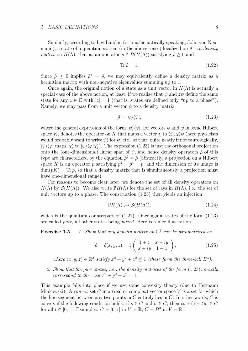
Exercise 1.5 1. Show that any density matrix on C2 can be parametrized as
ρ = ρ(x, y, z) = 12
(1 + z x− iyx+ iy 1− z
), (1.25)
where (x, y, z) ∈ R3 satisfy x2 + y2 + z2 ≤ 1 (these form the three-ball B3).
2. Show that the pure states, i.e., the density matrices of the form (1.23), exactlycorrespond to the case x2 + y2 + z2 = 1.
This example falls into place if we use some convexity theory (due to HermannMinkowski). A convex set C in a (real or complex) vector space V is a set for whichthe line segment between any two points in C entirely lies in C. In other words, C isconvex if the following condition holds: if ρ ∈ C and σ ∈ C, then tρ+ (1− t)σ ∈ Cfor all t ∈ [0, 1]. Examples: C = [0, 1] in V = R, C = B3 in V = R3.

1 BASIC DEFINITIONS 9
Exercise 1.6 1. Show that the classical state space P(EΛ) is convex.
2. Show that the quantum state space S(H(Λ)) is convex.
The extreme boundary ∂eC of a convex set C is the set of all extreme points ω ∈ C,defined by the following condition: if ω = tρ + (1 − t)σ for some 0 < t < 1 andρ, σ ∈ C, then ρ = σ = ω. In other words, an extreme point cannot lie on a linesegment inside C (except as an endpoint). As first proposed by von Neumann, inphysics the pure states are precisely the extreme points of the state space. This ideais justified by seeing pure states as states about which we have maximal information;mixed states, on the other hand, are obtained by combining pure states with weightscorresponding to (subjective) probabilities. Indeed, iterating the definition of aconvex set it follows that if points ωi lie in C (i = 1, . . . , n) and probabilities pi ∈[0, 1] sum to 1 (as they should), then
∑i piωi lies in C. Conversely, one may ask if
all points in some convex set may be written as weighted sums of pure states. Thisturns out to be the case if C is compact, and if we allow suitably convergent infinitesums in the mixing operation. Clearly, under these conditions the pure state spacecannot be empty.6
Exercise 1.7 1. Let M2(C) → C be the set of 2 × 2 complex matrices. Eachdensity matrix ρ on C2 defines a map ω : M2(C)→ C by
ω(a) = Tr (ρa). (1.26)
(a) Show that ω is linear (trivial), that ω(1) = 1 (almost trivial), and thatω(a) ≥ 0 for all a ≥ 0 (easy).
(b) Conversely, show that any linear map ω : M2(C) → C that satisfies thelatter two conditions is necessarily of the form (1.26), where ρ is somedensity matrix on C2.
This exercise leads to a unified picture of states of classical and quantum systems.We start with the algebra of observables A, or any local subalgebra A(Λ) thereof, anddefine a state as a linear map ω : A → R (classically) or ω : A → C (quantummy)that satisfies the two conditions in the previous exercise, i.e. ω(1) = 1 and ω(a) ≥ 0for all a ≥ 0. It immediately follows that the set of all states thus defined is convex.7
The physical interpretation of a state is simply that ω(a) is the expectation valueof an observable a ∈ A in the state ω; in other words, a state is now regarded asa rule that tells any observable what its expectation value is. In classical physics,8
the Riesz–Markov Theorem of measure theory shows that this notion of a state is
6This is the Krein–Milman Theorem from functional analysis. A simple example of a convex setwith empty extreme boundary is the three-ball without its boundary, which indeed is non-compact!
7It is also compact as a subset of the dual space A∗ of continuous linear functionals on A, butonly if A∗ is equipped with the so-called weak-star topology.
8Here it is crucial that classical observables in A are localized, which implies that they arecontinuous functions on EZd
. Otherwise, the Riesz–Markov Theorem does not apply.

1 BASIC DEFINITIONS 10
equivalent to the one we had, i.e., any state ω is given by a probability distributionp, according to
ω(f) =∑s∈EZd
p(s)f(s) ≡ 〈f〉p. (1.27)
In quantum physics, a generalization of Exercise (b) above shows that for finite-dimensional Hilbert spaces the new notion of a state just recovers the old notionof a density matrix, in that any state is given by (1.26). The true value of ournew definition of a state emerges for infinite quantum systems: since (unlike itssubalgebras A(Λ)) the algebra A of local observables no longer acts on any Hilbertspace, the whole notion of a density matrix becomes obscure.
1.3.3 Equilibrium states of finite systems
Arguably the most interesting states in physics are equilibrium states, defined withrespect to some temperature T (whose deeper mening shall remain obscure in thesenotes). We first defines such states locally, i.e., in a finite lattice Λ ⊂ Zd.
Classically, given an interaction Φ and the ensuing family of local HamiltonianshΛ, we define the local energy for each Λ as a function EΛ : P(EΛ) → R of theclassical states on EΛ, i.e., of the probability distributions on EΛ, by
EΛ(p) =∑s∈EΛ
p(s)hΛ(s). (1.28)
Of course, this is just the expectation value of the Hamiltonian in the state p, cf.(1.27). The local entropy SΛ : P(EΛ)→ R is a more subtle concept; rather than theexpectation value of some (local) observable, it yields a property of the probabilitydistribution itself. With Boltzmann’s constant kB, we have
SΛ(p) = −kB∑s∈EΛ
p(s) ln(p(s)). (1.29)
Note that SΛ(p) ≥ 0, with equality iff p is a pure state.Finally, the local free energy FβΛ : P(EΛ)→ R is then defined as
FβΛ = EΛ − TSΛ, (1.30)
where β = 1/kBT . A local equilibrium state, then, is a probability distribution pβΛthat minimizes the free energy (for fixed T ). Boltzmann’s solution is given by
pβΛ(s) = (ZβΛ)−1e−βhΛ(s); (1.31)
ZβΛ =
∑s′∈EΛ
e−βhΛ(s′). (1.32)
Exercise 1.8 Show that FβΛ(p) ≥ −β−1 lnZβΛ for all p, with equality iff p = pβΛ.
Here “for all p” of course means for all p ∈ P(EΛ). It follows that there is a uniquelocal equilibrium state for each T , with ensuing free energy in equilibrium
F βΛ = FβΛ(pβΛ) = −β−1 lnZβ
Λ. (1.33)
Note that none of the above expressions makes sense for Λ = Zd, but one mighthope that the corresponding intensive quantities (like fβΛ = F β
Λ/|Λ|) have a limit.

1 BASIC DEFINITIONS 11
The corresponding quantum-mechanical expressions are the same, mutatis mu-tandis. In particular, the energy EΛ, entropy SΛ, and free energy FβΛ are now func-tions on the space S(H(Λ)) of the density matrices on H(Λ). We have
EΛ(ρ) = Tr (ρhΛ); (1.34)
SΛ(ρ) = −kBTr (ρ ln ρ); (1.35)
FβΛ = EΛ − T SΛ, (1.36)
ZβΛ = Tr e−βhΛ . (1.37)
If we define a local equilibrium state as a density matrix ρβΛ that minimizes the freeenergy (for fixed T ), the unique solution is given by the density matrix
ρβΛ = (ZβΛ)−1e−βhΛ . (1.38)
Exercise 1.9 Show that FβΛ(ρ) ≥ −β−1 ln ZβΛ for all ρ, with equality iff ρ = ρβΛ.
What remains to be done, however, is to define ground states and equilibrium statesfor infinite systems.
1.3.4 Ground states of infinite classical systems
The classical case is easy: with local Hamiltonians hΛ (or hbΛ, in case of a fixedboundary condition b) defined by a single interaction Φ according to (1.3) (or (1.4)),a ground state for Φ is simply a point s0 ∈ EZd
, i.e., a function s0 : Zd → E, whoserestriction (s0)|Λ to Λ minimizes hΛ (or hbΛ), for each finite Λ ⊂ Zd. In the Isingmodel in any d with B = 0 and free boundary condition, this gives the usual twoground states (in which all spins are either “up” or “down”).
Some authors (e.g., [6], however, use a slightly different notion for Hamiltonians(1.3) determined by free boundary conditions: they say that s0 ∈ EZd
is a groundstate for a given interaction Φ if, writing hs0Λ for (1.4) with b = s0, the condition
hs0Λ (s0) ≤ hs0Λ (s) (1.39)
holds for all finite Λ ⊂ Zd and all s ∈ EZdthat coincide with s0 outside Λ. In other
words, s0 itself acts as its own boundary condition b and this boundary condition isfixed for all s that compete with s0 in minimizing the local Hamiltonian hb=s0Λ . Thisdefinition opens the possibility of domain walls. For example, in the Ising model ind = 1 with B = 0, this definition admits ground states in which infinite chains of“spin up” alternate with infinite chains of “spin down”, and similarly in higher d.
Ground states may not exist and if they do, they may not be unique. Let us,therefore, briefly look at the set of ground states (for some fixed interaction). If this
set has at least two elements, say s(1)0 and s
(2)0 , then for any t ∈ (0, 1) we may form
the mixed state p0 = ts(1)0 + (1 − t)s(2)
0 , reinterpreted as a probability distribution
on EZdassigning probability t to s0 = s
(1)0 , probability (1 − t) to s = s
(2)0 , and
probability zero to all other points of EZd. Restricting ourselves to free boundary
conditions for simplicity, this state satisfies
〈hΛ〉p0 ≤ 〈hΛ〉p (1.40)

1 BASIC DEFINITIONS 12
for all probability distributions p on EZd. Hence we may relax the definition of a
ground state so as to admit mixed states, i.e., probability distributions p on EZd,
and say that p0 ∈ P(EZd) is a ground state if (1.40) holds for any p ∈ P(EZd
). Itfollows that the set G(Φ) of ground states of a given interaction Φ is a convex set,whose extreme points are the “pure ground states”. The above discussion suggeststhat these are pure states according to our original definition, that is, we would liketo identify ∂eG(Φ) with G(Φ)∩ ∂eP(EZd
) = G(Φ)∩EZd. Under suitable hypotheses
on Φ this is correct, and we may unambiguously talk about “pure ground states”.
1.3.5 Ground states of infinite quantum systems
The above definition of a classical ground state suggests that also in the quantumcase we may define a ground state of an infinite system as a state ω whose localizationωΛ to any finite volume |Λ| < ∞ (i.e., ωΛ is the restriction of ω : A → C toA(Λ) ⊂ A) is a ground state for hΛ. Surprisingly, such a naive definition would beinappropriate because of the superposition principle.
For example, we will see later on that in any finite volume Λ and 0 < B < Bc,the quantum Ising model (1.17) has a unique ground state ΨB
0 , as opposed to thecase B = 0, where it has two degenerate ground states ΨB=0
± , namely the obviousones with either all spins up or all spins down. Seen as states in the Hilbert space`2(EΛ), the functions ΨB=0
± are given by ΨB=0± = δs± , i.e., ΨB=0
± (s) = 0 for all s 6= s±and ΨB=0
± (s±) = 1, where s±(x) = ±1 for all x ∈ Λ. Roughly speaking, ΨB0 peaks
above both s+ and s−, like the wave function of the ground state of a symmetricdouble well potential, or, indeed, like the state of Schrodinger’s Cat.
However, in infinite volume the symmetry between s+ and s− (or the one σzi 7→−σzi in the Hamiltonian (1.17)) will be broken, so that, as in the finite-volume modelwith B = 0, there are two different ground states, one with all spins up and theother with all spins down.9 The point, then, is that the restriction of either of thosestates to finite Λ obviously fails to be of the above “Schrodinger Cat” form, so thatit cannot be a ground state of hΛ.
The correct definition of a ground state relies on the existence of the Heisenbergequation in infinite volume. Recall that in finite volume, this equation reads
da(t)
dt= i[hΛ, a(t)]. (1.41)
Setting t = 0, this defines a map δΛ : A(Λ) → A(Λ) by δΛ(a) = i[hΛ, a], which is aso-called derivation.10 We now assume that for each a ∈ A (i.e., a ∈ A(Λ) for some
9One way of seeing this is that tunneling between the two classical ground states in finite Λ issuppressed by ∼ exp(−|Λ|).
10For any algebra A, a derivation is a linear map δ : A→ A such that δ(ab) = δ(a)b+ aδ(b). Inclassical physics A is a commutative algebra of functions on phase space, and the derivative (w.r.t.either time or some spatial variable) provides an example of a derivation. In quantum physics, asfirst recognized by Dirac, taking the commutator defines a derivation, as in δ(a) = i[h, a]. Thefactor i is useful in case that h∗ = h, because in hat case we have δ(a∗) = δ(a)∗. Such a derivationis called symmetric, hermitian, or self-adjoint.

1 BASIC DEFINITIONS 13
finite Λ) the following limit exists:
δ(a) = i limΛ↑Zd
[hΛ, a]. (1.42)
If the interaction Φ has short range, in that spins within Λ only interact with a finitenumber of spins (within Λ or elsewhere), this will be certainly by the case, because
[A(Λ1), A(Λ2)] = 0 if Λ1 ∩ Λ2 = ∅, A(Λi) ⊂ A. (1.43)
More precisely, this locality property somewhat symbolically states that if a ∈ A(Λ1)and b ∈ A(Λ2), then [a, b] = 0. Indeed, although the sum in (the quantum analogueof) (1.3) has increasingly many terms as Λ ↑ Zd, for fixed a ∈ A(Λ) in (1.42) onlyfinitely many terms will contribute to the commutator.
Exercise 1.10 Prove(1.43) from the definition of A(Λ) = B(H(Λ)).
If the limit in (1.42) exists for some interaction Φ and ensuing local HamiltonianshΛ, we define a ground state as a state ω0 : A→ Λ that for all a ∈ A satisfies
−iω0(a∗δ(a)) ≥ 0. (1.44)
To justify this definition, let us assume we have a Hamiltonian h on some finite-dimensional Hilbert space H. By adding a constant if necessary, we may assumethat its lowest eigenvalue of h is E0 = 0, so that h ≥ 0 in the usual sense that
〈ψ, hψ〉 ≥ 0 (1.45)
for all ψ ∈ H. If some unit vector ψ0 satisfies
hψ0 = 0, (1.46)
so that it is a ground state in the usual sense, then by (1.45) with ψ = aψ0 and(1.46) the associated state (in the algebraic sense)
ω0(a) = 〈ψ0, aψ0〉 (1.47)
has the property
−iω0(a∗δ(a)) = 〈ψ0, a∗(ha− ah)ψ0〉 = 〈aψ0, haψ0〉 ≥ 0.
Exercise 1.11 Show, conversely, that for any unit vector ψ ∈ H that does notsatisfy hψ = 0, the associated state ω(a) = 〈ψ, aψ〉 fails the condition (1.44).
Finally, we note that the discussion on the set of classical ground states in §1.3.4may be repeated almost verbatim: the set of ground states of a quantum system isa compact convex set, whose extreme points are pure states under reasonable con-ditions on the interaction. As we shall see, this is no longer the case for equilibriumstates, where the extreme points correspond to “pure thermodynamic phases”.

1 BASIC DEFINITIONS 14
1.3.6 Equilibrium states of infinite classical systems
Neither the local Hamiltonians (1.3) nor the local partition functions (1.32) have alimit as Λ ↑ Zd. The correct way to define equilibrium states of infinite classicalsystems was given in 1968 by Dobrushin and independently by Lanford and Ruelle.
To explain their solution, we need to recall conditional probabilities. So far, wehave used probability distributions p on S = EΛ or S = EZd
, which associate anumber p(s) ∈ [0, 1] to each s ∈ S, subject to the condition
∑s p(s) = 1. More
generally, a probability measure on a discrete set S is a function P : P(S) → [0, 1](where P(S) is the power set of S, i.e., the set of all subsets of S), satisfying
P (S) = 1; (1.48)
P (A ∪B) = P (A) + P (B) if A ∩B = ∅ (S finite); (1.49)
P (∪iAi) =∑i
P (Ai) if Ai ∩ Aj = ∅ (i 6= j) (S infinite), (1.50)
where (Ai)i is any countable family of subsets of S. Here s ∈ S is often called anoutcome (of some stochastic process), whereas A ⊂ S is called an event. Clearly, aprobability distribution p on S gives rise to a probability measure P on S by
P (A) =∑s∈A
p(s), (1.51)
whilst a probability measure P on S induces a probability distribution p on S by
p(s) = P (s). (1.52)
If P (B) > 0, the conditional probability of A given B is defined by
P (A|B) =P (A ∩B)
P (B). (1.53)
Now take some finite Λ ⊂ Zd, and pick a spin configuration s : Λ → E as wellas a boundary condition b : Λc → E. These defines events s ⊂ EZd
and b ⊂ EZdby
s = s′′ ∈ EZd | s′′|Λ = s; (1.54)
b = s′′′ ∈ EZd | s′′′|Λc = b, (1.55)
whose intersection s ∩ b = s′ consists of the single spin configuration s′ : Zd → Ethat coincides with s on Λ and coincides with b on Λc, or s′|Λ = s and s′|Λc = b.
Dobrushin, Lanford, and Ruelle, then, proposed that an equilibrium state of aninfinite (spin-like) system is given by a probability distribution pβ on EZd
whoseassociated conditional probabilities for any finite Λ, s, and b as above, are given by
P β(s|b) = (Zβ(b))−1e−βhΛ(s|b), (1.56)
where P β is defined in terms of pβ by (1.51), hΛ(s|b) is given by (1.8), and
Zβ(b) =∑s∈EΛ
e−βhΛ(s|b). (1.57)
Exercise 1.12 Let Λ′ ⊃ Λ be finite, but large enough that spins in Λ do not interactwith spins outside Λ′. Show that the probability distribution pβΛ′, defined as in (1.31),satisfies (1.56) if Zd is replaced by Λ′ in the explanation after (1.53).

1 BASIC DEFINITIONS 15
1.3.7 Equilibrium states of infinite quantum systems
Attempting to define an equilibrium state of an infinite quantum system as a statewhose restriction to finite volume is an equilibrium state of the ensuing finite systemis unsatisfactory for the same reason as for ground states. The correct definitiononce again relies on the possibility of defining dynamics in infinite volume, but nowwe assume that for each a ∈ A the limit
a(t) = limΛ↑Zd
eithΛae−ithΛ (1.58)
exists. Although mathematically speaking this condition is slightly different fromthe existence of the limit in (1.42), as before (and for the same reason) it is satisfiedby short-range interactions. We assume this is the case, so that a(t) exists.
Roughly speaking, a KMS-state (named after Kubo, Martin, and Schwinger) onA at fixed inverse temperature β ∈ R is a state ω : A→ C that for all a, b ∈ A andall t ∈ R satisfies
ω(a(t)b) = ω(ba(t+ iβ)). (1.59)
This definition is correct for finite systems i.e., for A(Λ) instead of A, but for infinitesystems the following more precise formulation is needed: A KMS-state at inversetemperature β ∈ R is a state ω on A with the following property:
1. For any a, b ∈ A, the function Fa,b : t 7→ ω(ba(t)) from R to C has an analyticcontinuation to the strip Sβ = z ∈ C | 0 ≤ Im (z) ≤ β, where it is holomor-phic in the interior and continuous on the boundary ∂Sβ = R ∪ (R + iβ);
2. The boundary values of Fa,b are related, for all t ∈ R, by
Fa,b(t) = ω(ba(t)); (1.60)
Fa,b(t+ iβ) = ω(a(t)b). (1.61)
This precise definition shows a typical phenomenon for quantum statistical mechan-ics: time is no longer real, but takes values in the strip Sβ. For β →∞, i.e., T → 0,this strip becomes the entire upper half plane in C. In the opposite limit β → 0, orT →∞, a KMS-state obviously becomes a trace, in that ω(ab) = ω(ba).
Exercise 1.13 1. Define a state ωβΛ on A(Λ) = B(H(Λ)) by
ωβΛ(a) = Tr (ρβΛa), (1.62)
where the density matrix ρβΛ is given by (1.38). Show that ωβΛ satisfies (1.59).
2. Conversely, show that ρβΛ is the only density matrix whose associated state(1.26) satisfies (1.59).
3. For arbitrary operators a and b and state ω, define
Lab(t) = iω([a(t), b]); (1.63)
Cab(t) = ω([a(t), b]+), (1.64)

1 BASIC DEFINITIONS 16
where [a, b]+ = ab+ ba. Prove the fluctuation-dissipation theorem:11
If ω is an equilibrium state (i.e., a KMS-state) at inverse temperature β, then
Lab(ω) = i tanh( 12βω)Cab(ω), (1.65)
where the Fourier transform f of an arbitrary function f of t is defined as
f(t) =
∫ ∞−∞
dt e−iωtf(t). (1.66)
It follows from this exercise that for finite systems the KMS-condition is equivalentto the condition that a state minimizes the free energy, so that the KMS-conditioncharacterizes thermal equilibrium states. As first proposed by Haag, Hugenholtz,and Winnink in 1967, the KMS-condition defines thermal equilibrium states alsoin infinite systems, where the free energy is infinite. This definition has proven itsvalues in all subsequent studies of physical models. It has also led to the correct def-inition of pure thermodynamic phases, namely as the extreme points of the compactconvex set of KMS-states Kβ (at fixed temperature).12
The original relationship between equilibrium states and the free energy remainsvalid for infinite systems, in the sense that KMS-states minimize the intensive freeenergy fβ : S(A)→ R (where S(A) is the (compact convex) set of all states on A),given by
fβ(ω) = limΛ↑Zd
1
|Λ|FβΛ(ω|Λ), (1.67)
where FβΛ is given by (1.30), and we assume that the limit exists. Consequently, ifωβ is any KMS-state, and
F βΛ = −β−1 ln Zβ
Λ, (1.68)
we have
fβ := limΛ↑Zd
1
|Λ|F β
Λ = fβ(ωβ). (1.69)
There are many other characterizations and good properties of KMS-states, forwhich we refer to the literature [4, 11, 12].
11Through the linear response theory of Kubo, the function Lab is related to the influence of “dis-sipative” external influences on the system, whereas Cab is the two-point function for equilibriumfluctuations. The fluctuation-dissipation theorem is even equivalent to the KMS-condition.
12In contrast to ground states, extreme points ω ∈ ∂eKβ are never pure states.

2 ANSWERS TO SELECTED EXERCISES 17
2 Answers to selected exercises
Exercise 1.3. We first recall that if some Hilbert space K has an orthonormal basis(es)s∈S, (assumed to be finite or at most countable), then there is a unitary operatorU : K → `2(S). Indeed, we simply define U by linear extension of Ues = δs, whereδs(t) = δst. In other words, U(
∑s∈S cses) = c with c(s) = cs, where
∑s∈S |cs|2 <∞.
Let K = H(Λ) and S = EΛ, with E = 1, 2, . . . , n. In terms of the standardbasis (e1, . . . en) of H = Cn (any other basis might be used here, too), S now labelsthe specific orthonormal basis (es)s∈S of H(Λ) defined by es = ⊗x∈Λes(x), wherees(x) = es(x); recall that s ∈ S is a function s : Λ→ E.
Combining everything, we see that U : H(Λ)→ `2(S) defined by linear extensionof es 7→ δs, or, explicitly, U(
∑s∈EΛ cs ⊗x∈Λ es(x)) = c, with c(s) = cs, is unitary.
Exercise 1.8. We need to show that FβΛ(p) ≥ −β−1 lnZβΛ with equality iff p = pβΛ,
or, using (1.30), (1.28), and (1.29), that∑s∈EΛ
p(s)(hΛ(s) + β−1 ln p(s)) + β−1 lnZβΛ ≥ 0. (2.70)
Using (1.31), for each s ∈ EΛ we obtain
hΛ(s) = −β−1 lnZβΛ − β
−1 ln pβΛ(s). (2.71)
Substituting this in (2.70), using∑
s p(s) = 1, omitting the ensuing prefactor β−1,
and noting that pβΛ(s) > 0 for all s, the inequality (2.70) to be proved becomes
∑s∈EΛ
p(s) ln
(p(s)
pβΛ(s)
)≥ 0. (2.72)
Hence we need to prove the inequality
∑s∈EΛ
pβΛ(s) ·
(p(s)
pβΛ(s)
)ln
(p(s)
pβΛ(s)
)≥ 0, (2.73)
with equality iff p(s) = pβΛ(s) for all s.Let us now note that the function f(x) = x lnx is strictly convex for all x ≥ 0,
that is, for any finite set of numbers p′(s) ∈ (0, 1) with∑
s p′(s) = 1 and any set of
positive real numbers (xs)s ≥ 0, we have∑s
p′(s)f(xs) ≥ f(∑s
p′(s)xs), (2.74)
with equality iff all numbers xs are the same. Applying this with p′(s) = pβΛ(s) andxs = p(s)/pβΛ(s), so that p′(s)xs = p(s) and hence
∑s p′(s)xs =
∑s p(s) = 1, which
makes the right-hand side of (2.74) vanish since ln(1) = 0, finally leads to (2.73).Equality arises iff p(s)/pβΛ(s) equals the same numer c for all s; summing over all sforces c = 1, so that one has equality iff p(s) = pβΛ(s) for all s, as desired.

3 MEAN FIELD THEORY 18
3 Mean Field Theory
Exercise 3.1 1. Check (3.8) on p. 25 of Parisi.
2. Verify Parisi’s assertion that the free energy Φ = Φ(mi) in (3.8) is minimizediff mi = m for all i ∈ Λ, for a suitable m ∈ [−1, 1]. Here Parisi’s Φ[P ] is ourFβΛ(p).
3. From this result, assuming that mi = m for all i ∈ Λ, verify that for small m:
f(β, h) = −hm+ ( 12T −DJ)m2 +
T
12m4 +O(m6). (3.75)
Parisi’s (3.16) is the Bogoliubov inequality for the exact free energy:
F ≤ F0 + 〈h− h0〉0, (3.76)
where (for fixed Λ and β) for the sake of readability we have omitted all suffixes Λand β, so that F equals F β
Λ as defined in (1.33), (1.31), and (1.32), F0 is defined by(1.33) with h in (1.31) and (1.32) replaced by any “trial Hamiltonian” h0, and
〈a〉0 =∑s∈EΛ
p0(s)a(s), (3.77)
with p0 as defined in (1.31) and (1.32) with, once again, h replaced by h0.
Exercise 3.2 Show that F0 + 〈h− h0〉0 = FβΛ(p0), cf. (1.30), and argue that (giventheses lecture notes) Parisi’s convexity proof of (3.76) is unnecessary.
4 Low- and High-Temperature expansions
4.1 Low T
To begin with, we take the Hamiltonian for the Ising model in zero external field:
hΛ(s) = −J∑〈ij〉Λ
sisj. (4.78)
Introducing the set B(Λ) of all nearest-neighbour pairs within Λ, we typically writeb for some specific pair i, j ∈ B(Λ), and accordingly, s(b) = sisj. Also, define amap γ : EΛ → P(B(Λ)), where P(X) is the power set of some set X (that is, the setof all subsets of X; N.B. we write |X| for the number of elements of a set X), by
γ(s) = b ∈ B(Λ) | s(b) = −1. (4.79)
We may then rewrite the partition function (1.32) in finite Λ ⊂ ZD as
ZβΛ =
∑s∈EΛ
e−βhΛ(s) =∑s∈EΛ
eβJP〈ij〉Λ
sisj =∑s∈EΛ
eβJP
b∈B(Λ) s(b)
=∑s∈EΛ
eβJP
b∈B(Λ)(s(b)−1+1) = eβJ |B(Λ)|∑s∈EΛ
eβJP
b∈B(Λ)(s(b)−1)
= eβJD|Λ|∑s∈EΛ
e−2βJ |γ(s)| = 2eβJD|Λ|∑
B∈γ(EΛ)
e−2βJ |B|. (4.80)

4 LOW- AND HIGH-TEMPERATURE EXPANSIONS 19
With t = exp(−4βJ , it follows from (4.80) and (1.69) that, taking into account theempty set B = ∅, the intensive free energy is given by
fβ = −JD − β−1 limΛ↑Zd
1
|Λ|ln
1 +∑
B∈γ(EΛ)
t|B|/2
. (4.81)
Expanding the logarithm as ln(1 + x) = x − x2/2 + x3/3 − · · · yields the low-temperature expansion of the free energy. This expansion is difficult, because thesum over B interferes with the power series expansion of ln.
Exercise 4.1 1. Reproduce Parisi’s (4.6) on p. 48 from (4.81).
2. Generalize the derivation of (4.81) for Hamiltonians of the form
hΛ(s) = −∑b∈B(Λ)
J(b)s(b), (4.82)
where J : B(Λ)→ R is some function.
4.2 High T
It is instructive to start with a naive high-T expansion for the Ising model, that is,
ZβΛ =
∑s∈EΛ
eβJP〈ij〉Λ
sisj =∑s
∏〈ij〉Λ
eβJsisj (4.83)
=∑s
∏〈ij〉Λ
∞∑n=0
(βJ)n
n!snxs
ny =
∑s
∏b∈B(Λ)
∞∑n=0
(βJ)n
n!s(b)n
=∑s
∑ν∈NB(Λ)
∏b
(βJ)νb
νb!s(b)νb =
∑ν
(βJ)P
b νb∏b νb!
∑s
∏x∈Λ
sν(x)x
= 2|Λ|′∑ν
(βJ)P
b νb∏b νb!
≡ 2|Λ|∑G
w(G)(βJ)|G|. (4.84)
Here ν(x) =∑
b3x νb, the restricted sum∑′
ν is over all configurations ν : B(Λ)→ Nfor which ν(x) is even for each x ∈ Λ, and the final sum is over all topologicallydifferent graphs G in Λ with associated weights w(G) and length |G|. In this case, agraph is just a collection of lines drawn between nearest-neigbour vertices 〈ij〉 of Λ,subject to the rules that any number ν〈ij〉 ∈ N of lines may be drawn (including zero),and that the number of lines terminating at each vertex i must be even (includingzero). The weight w(G) is the product of
∏b∈G νb! and the number of distinct ways
a graph of the given topological type may be drawn inside Λ.For example, the empty graph has weight w(∅) = 1. The graph = consisting
of two lines between some nearest-neighbour pair has weight w( = ) = 12D|Λ|.
The idea, then, is that for high T (= low β) only small graphs (i.e., graphs for which|G| is small) contribute significantly to the expansion (4.84).

4 LOW- AND HIGH-TEMPERATURE EXPANSIONS 20
Exercise 4.2 1. Compute the coefficient of β4 in ZβΛ in any D.
2. Compute the free energy to order β4 and verify that lnZβΛ ∼ |Λ| to this order.
A simpler high-T expansion for the Ising model arises if we introduce the variablet = tanh(βJ), cf. [?, ?]. The result is
ZβΛ · 2
−|Λ|(cosh(βJ))−D|Λ| =′∑
ν∈2B(Λ)
tP
b νb ≡∑G
w(G)t|G|. (4.85)
where 2 = 0, 1, so that this time only graphs consisting of single lines betweennearest-neigbour vertices contribute, still subject to the rule that ν(x) (i.e., thenumber of lines terminating at vertex x–now either zero or one) be even for eachx ∈ Λ. This implies that only closed paths contribute, and w(G) just counts thenumber of ways G may be drawn. Apart from the empty graph, this process startsat |G| = 4, for which only one type of graph exists, namely the elementary square or‘plaquette’. For order |G| = 8 and higher, both connected and disconnected graphscontribute (even to the free energy).
Exercise 4.3 Compute (4.85) to order t4, compute the corresponding free energy toorder β4, and verify consistency with the previous exercise.
4.3 Gaussian model
See Parisi [?], §4.2.
Exercise 4.4 1. Find the ‘critical’ value of β for which the N × N (N = |Λ|)matrix A = I− βJ defining the Gaussian model loses positive definiteness.
2. Prove the last equation in (4.14), p. 50, of Parisi.

5 RENORMALIZATION GROUP 21
5 Renormalization Group
Theory: Mussardo Ch. 8.
Exercise 5.1 This exercise is about the classical Ising model in D = 1, with theusual variables si = ±1, i = 1, . . . , N (assumed even), K = βJ and h = 0, so that
−βhN(s) = K
N∑i=1
sisi+1. (5.86)
1. Show that ∑si=±1,i even
e−βhN (s) = e−βh′N/2
(s′), (5.87)
where
−βh′N/2(s′) =
N/2∑i=1
(K ′s′is′i+1 +K ′ + ln(2)), (5.88)
and, in terms of L = exp(2K), so that L ∈ [1,∞] as K ∈ [0,∞],
L′ = 12(L+ L−1). (5.89)
2. Show that the fixed point L∗ = 1 (i.e., L′∗ = L∗) is attractive, whereas the fixedpoint L∗ = ∞ is repelling (so that the renormalization flow is from L = ∞towards L = 0, or from T = 0 to T =∞).
3. Assuming N/3 ∈ N, repeat this analysis summing over all spins except nos. 2,5, 8, 11, . . . , using periodic boundary conditions (in other words, of each blockspin of three, keep the middle one and sum over the rest). Show, e.g., that
−βh′N/3(s′) =
N/3∑i=1
(K ′s′is′i+1 + g(K)), (5.90)
for suitable g(K), where this time, writing M = tanh(K), we have
M ′ = M3. (5.91)
4. Assuming N/(2l + 1) ∈ N, generalize the previous approach from block spinssized 3 to block spin sized 2l + 1, l ∈ N. The result looks like (5.90), but with
M ′ = M2l+1. (5.92)
Exercise 5.2 For general coupling constants K = (K1, . . . , Kn), write the RGtransformation induced by a block spin consisting of b original spins by K ′ = Rb(K).For some fixed point K∗, that is, Rb(K∗) = K∗, denote the eigenvalues of the n× nmatrix R′b(K∗) by λi(b). Show that λi(b1)λi(b2) = λi(b1b2), so that λi(b) = byi forsome ‘critical index’ yi (all critical exponents are expressible in terms of these yi).

6 EXACT SOLUTION OF THE QUANTUM ISING CHAIN 22
6 Exact solution of the quantum Ising chain
6.1 Fermionic Fock space and CAR
Let H be a Hilbert space and let F−(H) be the corresponding fermionic Fock space,i.e.,
F−(H) = ⊕∞n=0H⊗n− , (6.93)
where H⊗0 = C, and for n > 0 we have
H⊗n− = P(n)− H⊗n (6.94)
is the totally antisymmetrized n-fold tensor product of H with itself. Here theprojection P
(n)− : H⊗n → H⊗n is defined by linear extension of
P(n)− f1 ⊗ · · · ⊗ fn =
1
n!
∑π∈Sn
ε(π)fπ(1) ⊗ · · · ⊗ fπ(n), (6.95)
where SN is the permutation group on n objects and ε(π) is +1/ − 1 if π is aneven/odd permutation. On the usual Fock space
F (H) = ⊕∞n=0H⊗n, (6.96)
for each f ∈ H we define the usual annihilation operator a(f) by linear extension of
a(f)f1 ⊗ · · · ⊗ fn =√n(f, f1)H ⊗ · · · ⊗ fn, (6.97)
for n > 0, with a(f)z = 0 on H⊗0 = C, with adjoint a(f)∗ ≡ a∗(f) given by
a∗(f)f1 ⊗ · · · ⊗ fn =√n+ 1f ⊗ f1 ⊗ · · · ⊗ fn. (6.98)
Exercise 6.1 Show that (Ψ, a∗(f)Φ)F (H) = (Φ, a(f)Ψ)F (H) for all Φ,Ψ ∈ F (H).
For each f ∈ H, we then define the following operators on the fermionic Fock space:
c(f) = P−a(f)P−; (6.99)
c∗(f) = P−a∗(f)P−. (6.100)
Exercise 6.2 Show that c∗(f) = c(f)∗ and prove the anticommutation relations
[c(f), c∗(g)]+ = (f, g)H · 1; (6.101)
[c(f), c(g)]+ = 0; (6.102)
[c∗(f), c∗(g)]+ = 0. (6.103)
Of course, choosing an orthonormal basis (ei) of H and writing c(ei) = ci etc. yields
[ci, c∗j ]+ = δij · 1; (6.104)
[ci, cj]+ = 0; (6.105)
[c∗i , c∗j ]+ = 0. (6.106)
The algebra CAR(H) of Canonical Anticommutation Relations over H is the opera-tor algebra (technically, the C*-algebra) generated by the operators c(f) and c∗(f),f ∈ H, on F−(H).

6 EXACT SOLUTION OF THE QUANTUM ISING CHAIN 23
6.2 Jordan–Wigner transformation
The following fact is of great importance.
Proposition 6.3 If dim(H) = N <∞, then
F−(CN) = ⊕Nn=0H⊗n−∼= C2N
, (6.107)
andCAR(CN) ∼= M2N (C). (6.108)
Exercise 6.4 Prove (6.107) by a dimension count and prove (6.108) via Schur’sLemma: if A ⊂ Mk(C) is an algebra of matrices (i.e., A is closed under linearoperations, multiplication, and taking adjoints) containing the unit, then A = Mk(C)iff the only matrices that commute with all a ∈ A are multiples of the identity.
This result is important to us, because also
⊗NC2 ∼= C2N
, (6.109)
so that by Proposition 6.3,
F−(CN) = ⊗NC2; (6.110)
CAR(CN) ∼= M2N (C). (6.111)
This is already nontrivial for N = 1, in which case F−(C) ∼= C2, and, with a ≡ a(1),
a = σ− =
(0 01 0
); (6.112)
a∗ = σ+ =
(0 10 0
), (6.113)
gives a realization of CAR(C), with the usual notation σ± = 12(σx ± iσy).
To generalize this to arbitrary N > 1, we put a copy of the Pauli matrices oneach site i of a chain N = 1, 2, . . . , N, denoted by σµi , µ = 0, 1, 2, 3, with σ0 = 1.Following [8], for each i = 1, 2, . . . , N − 1 we then define operators
ci = eπiPi−1
j=1 σ+j σ−j σ−i ; (6.114)
c∗i = e−πiPi−1
j=1 σ+j σ−j σ+
i , (6.115)
along with c1 = σ−1 and c∗1 = σ+1 . Since
c∗i ci = a∗i ai =
(1 00 0
), (6.116)
the inverse transformation is given by
ai = e−πiPi−1
j=1 c∗j cjci; (6.117)
a∗i = c∗i eπi
Pi−1j=1 c
∗j cj . (6.118)

6 EXACT SOLUTION OF THE QUANTUM ISING CHAIN 24
More concretely, since the operators σ+j σ−j commute for different sites j, and
eπiσ+σ− =
(−1 00 1
), (6.119)
the so-called Jordan–Wigner transformation (6.114) - (6.115) is simply given by
ci =i−1∏j=1
(−1 00 1
)j
·(
0 01 0
)i
; (6.120)
c∗i =i−1∏j=1
(−1 00 1
)j
·(
0 10 0
)i
. (6.121)
Exercise 6.5 1. Defining
u =
( √1/2
√1/2
−√
1/2√
1/2
), (6.122)
and subsequently u(N) = ⊗Ni=1ui, show that
u(N)hNu∗(N) = h′N , (6.123)
where
hN = −JN∑i=1
σzi σzi+1 − Γ
N∑i=1
σxi ; (6.124)
h′N = −JN∑i=1
σxi σxi+1 − Γ
N∑i=1
σzi . (6.125)
2. Show that
h′N = 12ΓN − Γ
N∑i=1
c∗i ci − 14J
N∑i=1
(c∗i − ci)(c∗i+1 + ci+1) (6.126)
+ 14J(c∗N − cN)(c∗1 + c1)(eπi
PNj=1 c
∗j cj + 1). (6.127)
For large N , the term on the second line can be neglected (as it is bounded, unlikethe first) [8]. So we now show how to diagonalize quadratic fermionic Hamiltoniansof the type
hN =N∑
i,j=1
(Aijc
∗i cj + 1
2Bij(c∗i c∗j − cicj)
), (6.128)
where A and B are real N ×N matrices, with AT = A and BT = −B. This is doneby a so-called Bogoliubov transformation, whose abstract theory is as follows.

6 EXACT SOLUTION OF THE QUANTUM ISING CHAIN 25
6.3 Bogoliubov transformation
The passage (6.129) - (6.130) from operators c, c∗ satisfying the CAR, to new op-erators η, η∗ that also satisfy the CAR, as expressed in the following theorem, iscalled a Bogoliubov transformation.
Theorem 6.6 Let u and v be operators on a Hilbert space H, where u is linear andv is anti-linear (i.e., v(λΨ) = λv(Ψ) for λ ∈ C and Ψ ∈ H). Let c(f) and c∗(f) bethe operators (6.99) - (6.100), satisfying the CAR (6.101) - (6.103). Define
η(f) = c(uf) + c∗(vf); (6.129)
η∗(f) = c∗(uf) + c(vf). (6.130)
Then the canonical anticommutation relations
[η(f), η∗(g)]+ = (f, g)H · 1; (6.131)
[η(f), η(g)]+ = 0; (6.132)
[η∗(f), η∗(g)]+ = 0. (6.133)
hold if and only if u and v satisfy
uv∗ + vu∗ = v∗u+ u∗v = 0; (6.134)
u∗u+ v∗v = uu∗ + vv∗ = 1. (6.135)
Exercise 6.7 Prove this theorem.
Taking into account that c(f) is antilinear in f , whereas c∗(f) is linear, with respectto a base (ei) of H the Bogoliubov transformation (6.129) - (6.130) looks like
ηi =∑j
(ujicj + vjic∗j); (6.136)
η∗j =∑j
(ujic∗j + vjicj). (6.137)
6.4 Dynamics
With H = CN and ck := c(ek) and c∗k := c∗(ek), defined in terms of the usualorthonormal base (ek)
Nk=1 of CN , take the free Hamiltonian h on F−(CN) defined by
h =N∑k=1
εkc∗kck, (6.138)
where εk ≥ 0 for each k. Note that this is the second quantization of the single-particle Hamiltonian h(1) : CN → CN given by (linear extension of) h(1)ek = εkek.In this simple situation, the Heisenberg equations of motion for c and c∗ can beeasily solved, with the result that for arbitrary f ∈ CN we have
c(f)(t) ≡ eithc(f)e−ith = c(eith(1)
f); (6.139)
c∗(f)(t) ≡ eithc∗(f)e−ith = c∗(eith(1)
f). (6.140)

6 EXACT SOLUTION OF THE QUANTUM ISING CHAIN 26
In other words, we havec(f)(t) = c(f(t)), (6.141)
where f(t) solves the (anti) Schrodinger equation (−i instead of i)
−idf(t)
dt= h(1)f, (6.142)
with initial condition f(0) = f . As a special case, we obviously have
ck(t) = e−itεkck; (6.143)
c∗k(t) = eitεkc∗k. (6.144)
This remains true if H is infinite-dimensional, as long as the Hamiltonian h onF−(H) is the second quantization of some self-adjoint single-particle Hamiltonianh(1) : H → H (possibly even unbounded). One way to define what this means is:
Exercise 6.8 Given some self-adjoint single-particle Hamiltonian h(1) : H → H(assumed bounded for convenience), show that there is a self-adjoint operator h :F−(H) → F−(H), unique up to an additive constant, such that (6.139) - (6.140)hold. Also show that (6.138), (6.143), (6.144) is a special case of this construction.
However, most fermionic Hamiltonians are not in this form, even if they are quadraticin the c and c∗. In that case, h is diagonalizable by a Bogoliubov transformation,which means that there is a different fermionic Fock space (i.e., the one for which|0〉, the unit 1 of H⊗0 = C) satisfies η(f)|0〉 for all f ∈ H) on which h is thesecond quantization of some h(1). The simplest formalism to accomplish Bogoliubovtransformations for infinite-dimensional H is as follows.
6.5 Self-dual formalism
The self-dual formulation of the CAR, due to Araki, treats c and c∗ on equal footing.The advantage of this formalism is that formulae like (6.139) - (6.140) hold even if his not (already) of the form (6.138). The basic trick is to double H into K = H⊕H,with elements written h = (f, g) or h = f+g, indicating that f lies in the first copyof H, whereas g lies in the second. The inner product in K is given by
〈h1, h2〉K = 〈f1, f2〉H + 〈g1, g2〉H . (6.145)
We also need a conjugation on H, that is, an antilinear map J : H → H satisfyingJ∗ = J and J2 = 1. For H = `2(Z), the simplest example is
Jfi = fi. (6.146)
However, onH = L2([−π, π]) (6.147)
it turns out to be appropriate to use the Fourier transform of (6.146), which is
J ψ(k) = ψ(−k). (6.148)

6 EXACT SOLUTION OF THE QUANTUM ISING CHAIN 27
We then introduce the “field” (often called B instead of Φ)
Φ(h) = c∗(f) + c(Jg), (6.149)
which is linear in h = f+g, because the antilinearity of c(f) in f is canceled by theantilinearity of J . This yields
[Φ∗(h1),Φ(h2)]+ = 〈h1, h2〉K , (6.150)
but generally [Φ∗(h1),Φ∗(h2)]+ and [Φ(h1),Φ(h2)]+ do not vanish! Indeed, in termsof the antilinear operator Γ : K → K, defined by
Γ =
(0 JJ 0
)(6.151)
we haveΦ∗(h) ≡ Φ(h)∗ = Φ(Γh). (6.152)
If we identify f ∈ H with f+0 ∈ K, we may reconstruct c and c∗ from Φ through
c∗(f) = Φ(f); (6.153)
c(f) = Φ(Γf). (6.154)
The self-dual formulation of Bogoliubov-transformations is now extremely elegant,as follows: for any unitary operator S on K that satisfies [S,Γ] = 0, we define aBogoliubov-transformed field
ΦS(h) = Φ(Sh), (6.155)
with associated creation- and annihilation operators (where H 3 f ≡ f+0, as above)
c∗S(f) = ΦS(f); (6.156)
cS(f) = Φ∗S(f). (6.157)
Exercise 6.9 Show that S necessarily has the form
S =
(u vJJv JuJ
), (6.158)
where u : H → H is linear and v : H → H is antilinear, and u and v satisfy (6.134)and (6.135). Subsequently, prove that cS(f) and c∗S(f) coincide with η(f) and η∗(f)in (6.129) and (6.130), respectively.
6.6 Diagonalizing the Hamiltonian
The point of all this is that we can now diagonalize the N → ∞ limit of theHamiltonian (6.128), or rather, for a two-sided chain (assuming N even)
hN =
N/2−1∑i,j=−N/2
(Aijc
∗i cj + 1
2Bij(c∗i c∗j − cicj)
), (6.159)

6 EXACT SOLUTION OF THE QUANTUM ISING CHAIN 28
This limit exist in the sense that, for H = `2 and any a ∈ CAR(H), the derivation
δ(a) = i limN→∞
[hN , a] (6.160)
is well defined, whilst also the Heisenberg-picture time evolution
a(t) = limN→∞
eithNae−ithN (6.161)
exists. Combining this, the operator Heisenberg equation
da(t)
dt= i lim
N→∞[hN , a(t)] (6.162)
is well defined and has a unique solution (6.161) subject to a(0) = a. The point is:
Exercise 6.10 Show that for any h ∈ K one has (cf. (6.141) - (6.142))
Φ(h)(t) = Φ(h(t)), (6.163)
where h(t) solves the ‘doubled’ (anti) Schrodinger equation
−idh(t)
dt= h
(1)D h, (6.164)
with initial condition h(0) = h. Here the ‘doubled’ one-particle Hamiltonian operator
h(1)D : K → K is given by
h(1)D =
(A B−B −A
), (6.165)
where A : `2(Z) → `2(Z) and B`2(Z) → `2(Z) are the obvious extensions of theN ×N matrices A and B to operators on `2(Z) (assuming the entries Aij and Bij
are defined whenever (i, j) ∈ Z× Z).
Exercise 6.11 Recall the finite-N Hamiltonian for the quantum Ising chain:
hIN = −N/2−1∑j=−N/2
(σxj σ
xj+1 + λσzj
), (6.166)
where we (conventionally) have put J = 1 and interchanged the x- and z-axes.
1. Show that for this Hamiltonian
A = 12(S + S∗)− λ; (6.167)
B = 12(S− S∗), (6.168)
where S : `2(Z)→ `2(Z) is the shift operator, defined on a sequence (fj) by
Sfj = fj+1; (6.169)
S∗fj = fj−1. (6.170)
Note that in terms of the standard basis (ej) of `2(Z) we have Sej = ej−1 andS∗ej = ej+1.

6 EXACT SOLUTION OF THE QUANTUM ISING CHAIN 29
2. Show that a Fourier transformation U : `2(Z)→ L2([−π, π]), given by
(Uf)(k) ≡ f(k) =∑j∈Z
e−ijkfj; (6.171)
(U−1f)j ≡ fj =
∫ π
−π
dk
2πeijkf(k), (6.172)
diagonalizes A and B to A, B : L2([−π, π])→ L2([−π, π]), given by
Aψ(k) = ((cos k)− λ)ψ(k); (6.173)
Bψ(k) = −i sin k ψ(k). (6.174)
3. For fixed k, show that the eigenvalues and eigenvectors of the 2× 2 matrix
Mk =
((cos k)− λ −i sin ki sin k −(cos k − λ),
)(6.175)
are ±εk, withεk =
√1 + λ2 − 2λ cos k. (6.176)
4. Show that the unitary 2× 2 matrix
Uk =
(uk vkvk uk
); (6.177)
uk = Nk sin k; (6.178)
vk = iNk(εk + λ− cos k), (6.179)
Nk = (1 + (εk + λ)2 − 2(εk + λ) cos k)−1/2 (6.180)
= (sin2 k + (εk + λ− cos k)2)−1/2. (6.181)
diagonalizes Mk in the sense that
U−1k MkUk =
(εk 00 −εk
). (6.182)
5. With K = H ⊕ H, where H = L2([−π, π]), we now turn Mk and Uk intomultiplication operators M and U on K in the obvious way, so that
M = h(1)D =
(A B
−B −A
), U =
(u vv u
), (6.183)
with A and B defined by (6.173) - (6.174), and uψ(k) = ukψ(k), etc. Prove
U−1MU =
(ε 00 −ε
), (6.184)
where ε : H → H is the multiplication operator defined by εψ(k) = εkψ(k).

6 EXACT SOLUTION OF THE QUANTUM ISING CHAIN 30
6.7 Ground states for the CAR-algebra
The fermionic Fock space F−(H) has a special state |0〉 for which 〈0|0〉 = 1 andc(f)|0〉 = 0, and all states in F−(H) are obtained by repeatedly acting on |0〉 withthe c∗(f) and taking linear combinations (and limits). More abstractly, the unitvector |0〉 defines a state ω0 : CAR(H)→ C on CAR(H) in the abstract sense by
ω0(a) := 〈0|a|0〉, a ∈ CAR(H). (6.185)
This state turns out to be a ground state for the simple time-evolution given by(6.143) - (6.144), or, equivalently, for the limiting dynamics defined by the finite-volume Hamiltonians (6.138) (though the sum should run as indicated below).
Exercise 6.12 1. With hN =∑N/2−1
k=−N/2 εkc∗kck and δ(a) := i[hN , a] as a deriva-
tion δ : CAR(CN)→ CAR(CN), show that ω0 is a ground state a la (1.44).
2. Show that there exists no other pure ground state on CAR(CN), and hence noother ground state whatsoever. You may use the fact that the construction
ψ(a) = 〈Ψa,Ψ〉, (6.186)
for some unit vector Ψ ∈ F−(H), yields all pure states on CAR(CN).
Now let N →∞, that is, replace CN by the Hilbert space `2(Z) of square-summablesequences of complex numbers. In that case, the algebra CAR(`2) and the fermionicFock space F−(`2) are still perfectly well defined, but a Hamiltonian like (6.138) willgenerally be unbounded. Nonetheless, the derivation
δ(a) := i limN→∞
[hN , a], (6.187)
is well defined, but only on operators a that are finite sums of products of finitelymany c’s and c′s. Of course, in this case (1.44) should only hold on such operators.
Exercise 6.13 Repeat the previous exercise for this situation.
From the point of view of the self-dual formalism, the above discussion merely coversthe case where h
(1)D is already diagonal on K = H ⊕H. In that case, the state |0〉
is characterized by the property c(f)|0〉 = 0 for all f ∈ H. In general, however, weneed to deal with the case (6.165). According to the previous two sections (especially(6.184), (6.158), and (6.146), and Exercise 6.9), the ground state is now given by(6.185), where this time the Fock space vacuum state is characterized by η(f)|0〉 = 0
for all f ∈ H, with η(f) =∫ π−π
dk2πηkf(k) (and hence η∗(f) =
∫ π−π
dk2πη∗kf(k)), where
ηk = ukck + vkc∗−k; η∗kukc
∗k + vkc−k; (6.188)
ck =∑j∈Z
e−ijkcj; c∗k =∑j∈Z
eijkc∗j , (6.189)
with uk, vk given by (6.178) - (6.179). It follows that [η(f), η∗(g)]+ = 〈f , g〉 (innerproduct in H) and [η±(f), η±(g)]+ = 0, so that also
ω0(η(f)η∗(g)) = 〈0|η(f)η∗(g)|0〉 = 〈f , g〉; (6.190)
ω0(η∗(f)η(g)) = 〈0|η∗(f)η(g)|0〉 = 0. (6.191)

6 EXACT SOLUTION OF THE QUANTUM ISING CHAIN 31
6.8 The GNS-construction
Algebras like CAR(H) and ⊗NM2(C), also for dim(H) =∞ and N =∞, are exam-ples of so-called C∗-algebras. In what follows, we will not give a formal definition ofsuch algebras but just use the facts that one can add and multiply the elements ofsuch algebras (which are to be thought of as operators), and that they have an invo-lution a 7→ a∗, which is an abstract version of the hermitian conjugate for matricesor, more generally, for operators on Hilbert space. In a more mathematical account,the fact that a C∗-algebra forms a Banach space plays a role, which is responsiblefor the fact that C∗-algebras can always be realized as algebras as bounded opera-tors on some Hilbert space. In any case, C∗-algebras make sense without referenceto a Hilbert space, although their construction or definition typically starts fromsome Hilbert space, like the fermionic Fock space F−(H) for CAR(H), or ⊗NC2 for⊗NM2(C) (where N < ∞). As will be clear from what follows, in many respectsC∗-algebras behave like groups, in that they are defined abstractly, upon which onemay look for concrete representations on vectors spaces, notably on Hilbert spaces.
Definition 6.14 A representation of a C∗-algebra A on a Hilbert space H is alinear map π : A→ B(H) such that π(ab) = π(a)π(b), and π(a∗) = π(a)∗, ∀a, b ∈ A.
• A representation π : A→ B(H) is called cyclic if there is a vector Ω ∈ H forwhich π(A)Ω = H;13 in other words, each Ψ ∈ H is the limit of a sequenceπ(an)Ω in H, where an ∈ A. In that case, Ω is called a cyclic vector for π.
Physically, the idea behind cyclicity would be that each state arises by ‘filling up’ theground state Ω with ‘excitations’ π(a)Ω. There is a beautiful connection betweencyclic representations of A and states on A, given by the GNS-construction.14 Inquantum physics, this construction provides the bridge between the usual Hilbertspace formalism and the abstract C∗-algebraic approach, so it is quite important.
Theorem 6.15 Let ω : A→ C be a state on a C∗-algebra A. There exists a cyclicrepresentation πω of A on a Hilbert space Hω with cyclic unit vector Ωω such that
ω(a) = 〈Ωω, πω(a)Ωω〉 ∀a ∈ A. (6.192)
The idea is to construct Hω from A and subsequently define πω by left-multiplication:
1. Define a sesquilinear form 〈−,−〉0 on A by
〈a, b〉0 := ω(a∗b). (6.193)
This form almost defines an inner product on A, except that it may not bepositive definite (i.e., it might be that ω(a∗a) = 0 for some a 6= 0, so that〈a, a〉0 = 0). Hence we remove the null space
Nω = a ∈ A |ω(a∗a) = 0 (6.194)
13Here π(A)Ω is the closure of the linear span of the subset π(a)Ψ, a ∈ A,Ψ ∈ H of H.14Named after three founding fathers of the field: I.M. Gelfand, M. Naimark, and I.E. Segal.

6 EXACT SOLUTION OF THE QUANTUM ISING CHAIN 32
by forming the quotient A/Nω. The form
〈[a], [b]〉 := ω(a∗b) (6.195)
on A/Nω (where [a] is a modulo elements of the null space Nω) is positivedefinite by construction and hence defines an inner product 〈−,−〉 on thecomplex vector space A/Nω. The Hilbert space Hω, then, is the completion ofA/Nω in the corresponding norm.
2. The representation πω(A) is initially defined on A/Nω ⊂ Hω by
πω(a)[b] := [ab]. (6.196)
It is trivial that πω is linear and satisfies πω(ab) = πω(a)πω(b); to prove thatπω(a)∗ = πω(a∗), take inner products with vectors [b] and [c] in A/Nω. Thetechnical point of the proof, which we omit, is that each πω(a) is well definedand bounded on A/Nω, so that it may be extended to all of Hω by continuity.
3. If A has a unit, which is the case in all our examples (but which is not partof the official definition of a C∗-algebra), define Ωω = [1]; then (6.192) followsby a simple computation:
〈Ωω, πω(a)Ωω〉 = 〈[1], [a1]〉 = ω(1∗a1) = ω(a).
We will usually drop the index ω and also omit the symbol π ≡ πω, so the the ω-dependence of the entire construction is hidden in the definition of the inner producton H. If we don’t bother about the fact that for infinite-dimensionla H, the spaceAΩ is just dense in H (and so strictly speaking does not coincide with H), we canwrite vectors in H as bΩ for some b ∈ A, so that the representation of A on H isjust given by a(bΩ) = abΩ, and the inner product on H is simply
〈aΩ, bΩ〉 = ω(a∗b). (6.197)
For example, take A = Mn(C), with a state necessarily of the form
ω(a) = Tr (ρa), (6.198)
for some density matrix ρ (as we have seen). Writing N for Nω, etc., it follows that
N = a ∈ A | Tr (ρa∗a) = 0. (6.199)
Exercise 6.16 In this example, assume for simplicity that ρ =∑n
i=1 λi|ei〉〈ei| withrespect to the standard basis (ei) of Cn (otherwise, change basis), Compute N , A/N ,and the representation π(A) on A/N in the following special cases:
1. λj = 1 for some j, so that ρ = |ej〉〈ej| is pure;
2. λi > 0 for all i (as in an equilibrium state ρ = Z−1 exp(−βh), where Z =Tr exp(−βh) for some Hamiltonian h : Cn → Cn).

6 EXACT SOLUTION OF THE QUANTUM ISING CHAIN 33
6.9 Irreducible representations and pure states
As for group representation, there are natural notions of equivalence and irreducibil-ity for representations of C∗-algebras.
Definition 6.17 Two representations π1 : A → B(H1) and π2 : A → B(H2) arecalled equivalent (π1
∼= π2) if there is a unitary operator u : H1 → H2 intertwiningπ1 and π2, in the sense that π2(a) = uπ1(a)u∗ for all a ∈ A.
Exercise 6.18 Show that (for fixed A) ∼= is an equivalence relation, in that:
1. π ∼= π for each representation π;
2. If π1∼= π2, then π2
∼= π1;
3. If π1∼= π2 and π2
∼= π3, then π1∼= π3.
Definition 6.19 A representation π : A → B(H) is called irreducible when Hhas no nontrivial closed subspaces stable under π(A). In other words, if K ⊂ H is aclosed subspace such that π(a)Ψ ∈ K for all a ∈ A, Ψ ∈ K, then K = 0 or K = H.
If π is not irreducible, then we do have such a subspace K, and since π(a∗) = π(a)∗
it follows that also K⊥ is stable under π. Thus we may reduce H = K ⊕ K⊥,with π(A)K(⊥) ⊂ K(⊥). For example, the defining representation of A = Mn(C) isirreducible, but its restriction to the algebra Dn of diagonal matrices is not: eachsubspace C · ei is stable under Dn.
Exercise 6.20 Show that if π1∼= π2 and π1 is irreducible, then so is π2.
The following result is analogous to Schur’s Lemma in group theory.
Theorem 6.21 The following conditions on π : A→ B(H)are equivalent:15
1. π is irreducible;
2. Each nonzero vector Ω ∈ H is cyclic;
3. π(A)′ = C · 1, or, equivalently, π(A)′′ = B(H).
To get some idea of the proof, if π(A)′ 6= C·1, then by advanced (functional) analysisπ(A)′ contains a nontrivial projection p, and hence the image K = pH of H underp is stable under A. This proves ¬3⇒ ¬1 and hence 1⇒ 3.
There is a beautiful characterization of irreducibility of GNS-representations,which in the theory of phase transitions will be the main technique (in combinationwith the previous theorem) for proving that some ground state is pure or mixed.
15Here the commutant M ′ of a collection M of bounded operators consists of all boundedoperators that commute with all elements of M , and the bicommutant M ′′ is simply the iteratedcommutant (M ′)′.

6 EXACT SOLUTION OF THE QUANTUM ISING CHAIN 34
Theorem 6.22 The GNS-representation πω(A) is irreducible iff ω is pure.Equivalently, ω is mixed iff there exists an operator b 6= λ·1 on Hω that commutes
with all operators πω(a) on Hω (informally: bacΩ = abcΩ for all a, c ∈ A).
Corollary 6.23 A state ω on A is pure iff πω(A)′ = C · 1.
We just prove the easy direction of the corollary: if πω(A)′ 6= C · 1, then ω is mixed.So suppose the commutant πω(A)′ is nontrivial. Again by functional analysis, it
then contains a nontrivial projection p+ ∈ πω(A)′ (so p+ 6= 1 and p+ 6= 0). It thenfollows that p+Ωω 6= 0: for if p+Ωω = 0, then ap+Ωω = p+aΩω = 0 for all a ∈ A, sothat p+ = 0, since πω is cyclic. Similarly, p−Ωω 6= 0 with p− = 1 − p+, so we maydefine the unit vectors
Ω± := p±Ωω/‖p±Ωω‖, (6.200)
and the associated statesω±(a) := 〈Ω±, πω(a)Ω±〉 (6.201)
on A. This yieldsω = λω+ + (1− λ)ω−, (6.202)
withλ = ‖Ω−‖2. (6.203)
Since λ 6= 0, 1 and ω+ 6= ω−, it follows that ω is mixed. The associated reduction iseffected by writing
H = H+ ⊕H−; (6.204)
H± = p±H, (6.205)
in that A (more precisely, πω(A)) maps each subspace H± into itself. Q.E.D.
Exercise 6.24 Continue the previous Exercise 6.4:
1. Prove that the state ρ = |ej〉〈ej| on A = Mn(C) is pure by computing thecommutant of the corresponding (GNS) representation;
2. If λi > 0 for all i in ρ =∑n
i=1 λi|ei〉〈ei|, prove that ρ is mixed by computingthe commutant of the corresponding (GNS) representation.
Exercise 6.25 Continue the previous Exercise 6.16: prove that the defining rep-resentation of CAR(H) on the fermionic Fock space F−(H) is irreducible, for anyHilbert space H (and not just for H = CN).

6 EXACT SOLUTION OF THE QUANTUM ISING CHAIN 35
6.10 Z2-actions
The± notation above is explained by passing from the projections p± to the operator
w = p+ − p−, (6.206)
so thatw∗ = w; w2 = 1. (6.207)
In particular, w is unitary. Conversely, if some unitary w satisfies w2 = 1, then
p± = 12(1± w) (6.208)
are projections satisfying p+ + p− = 1, giving rise to the decomposition (6.205).Group-theoretically, this means that one has a unitary Z2-action on H ≡ Hω, inwhich the nontrivial element of Z2 = −1, 1 is represented by w. The decompo-sition (6.205) then simply means that Z2 acts trivially on H+ (in that both groupelements are represented by the unit operator) and acts nontrivially H− (in that thenontrivial element is represented by minus the unit operator).
Thus instead of a projection p ∈ πω(A)′ , one may equivalently look for anoperator w ∈ πω(A)′ that satisfies (6.207).
Where group actions (i.e., unitary representations) on Hilbert spaces should befamiliar, it may be less familiar (but equally useful) to consider group actions on(C*) algebras. Such actions are defined in terms of so-called automorphisms.
Definition 6.26 An automorphism of A is an invertible linear map θ : A → Asatisfying θ(ab) = θ(a)θ(b) and θ(a∗) = θ(a)∗.
For example, if u ∈ A is unitary, in that uu∗ = u∗u = 1, then θ(a) = uau∗ definesan automorphism (check).
Definition 6.27 A Z2-action on A is an automorphism θ : A→ A with θ2 = id.
Similarly to the Hilbert space decomposition (6.204) under a Z2-action, an algebraA carrying a Z2-action decomposes as
A = A+ ⊕ A−; (6.209)
A± = a ∈ A | θ(a) = ±a. (6.210)
Here the so-called even part A+ is a subalgebra of A, whereas the odd part A− isnot: one has ab ∈ A+ for a, b both in either A+ or A−, and ab ∈ A− if one is in A+
and the other in A−. For example, if A consists of all bounded operators on someHilbert space H and w : H → H is a untitary operator satisfying w2 = 1, then
θ(a) = waw∗ (= waw) (6.211)
defines a Z2-action on A, where A+ and A− consist of all a ∈ A that commute andanticommute with w, respectively, that is,
A± = a ∈ A | aw ∓ wa = 0. (6.212)

6 EXACT SOLUTION OF THE QUANTUM ISING CHAIN 36
As another example, take the Fermion algebra
F = CAR(`2(Z)), (6.213)
generated by the operators c±j , j ∈ Z, c−j ≡ cj, c+j ≡ c∗j , subject to the usual CAR
[c±i , c∓j ]+ = δij, [c±i , c
±j ]+ = 0. Here we may define θ : F → F by
θ(c±j ) = −c±j , j ∈ Z, (6.214)
extended to all a ∈ F by the defining properties of an automorphism (which, forexample, imply θ(1) = 1). In this case, F+ (F−) is just the linear span of all productsof an even (odd) number of c±j ’s.
There is some sort of a converse to the construction (6.211) of a Z2-action.
Theorem 6.28 Suppose A carries a Z2-action θ and consider a state ω : A → Cthat is Z2-invariant in the sense that ω(θ(a)) = ω(a) for all a ∈ A. We write thisas θ∗ω = ω, with θ∗ω := ω θ. Then there is a unitary operator w : Hω → Hω
satisfying w2 = 1, wΩ = Ω, and and wπω(a)w∗ = πω(θ(a)) for each a ∈ A.
Informally: waw∗ = θ(a) on H. The idea of the proof is to define w on vectors ofthe type bΩ ≡ πω(b)Ωω (and thence on all vectors in H by continuity) by
wbΩ := θ(b)Ω. (6.215)
Taking b = 1 already gives wΩ = Ω, and w2 = 1 (and hence invertibility of w, inthat w−1 = w) follows from θ2 = id. Finally, unitarity follows from the computation
〈waΩ, wbΩ〉 = 〈θ(a)Ω, θ(b)Ω〉 = 〈Ω, θ(a)∗θ(b)Ω〉 = 〈Ω, θ(a∗)θ(b)Ω〉= 〈Ω, θ(a∗b)Ω〉 = ω(θ(a∗b)) = ω(a∗b) = 〈aΩ, bΩ〉.
In this situation, we obtain a decomposition of H ≡ Hω according to (6.204), wherethe projections p± are given by (6.208), so that, equivalently,
H± = Ψ ∈ H | wΨ = ±Ψ = A±Ω, (6.216)
the bar denoting closure. In terms of the decomposition (6.209), it is easily seen thateach subspace H± is stable under A+, whereas A− maps H± into H∓. We denote therestriction of πω(A+) to H± by π±, so that a Z2-invariant state θ on A not just givesrise to the GNS-representation πω of A on Hω, but also induces two representationsπ± of the even part A+ on H±. This leads to a refinement of Theorem 6.22 [3]:
Theorem 6.29 Suppose A carries a Z2-action θ as well as a Z2-invariant stateω : A → C. With the above notation, suppose the representation π+(A+) on H+
is irreducible. Then also the representation π−(A+) on H− is irreducible, and thereare the following two possibilities for the representation πω(A) on H = H+ ⊕H−:
1. πω(A) is irreducible (and hence ω is pure) iff π±(A+) are inequivalent;
2. πω(A) is reducible (and hence ω is mixed) iff π±(A+) are equivalent.
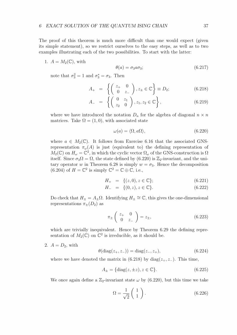
6 EXACT SOLUTION OF THE QUANTUM ISING CHAIN 37
The proof of this theorem is much more difficult than one would expect (givenits simple statement), so we restrict ourselves to the easy steps, as well as to twoexamples illustrating each of the two possibilities. To start with the latter:
1. A = M2(C), withθ(a) = σ3aσ3; (6.217)
note that σ23 = 1 and σ∗3 = σ3. Then
A+ =
(z+ 00 z−
), z± ∈ C
≡ D2; (6.218)
A− =
(0 z1
z2 0
), z1, z2 ∈ C
, (6.219)
where we have introduced the notation Dn for the algebra of diagonal n × nmatrices. Take Ω = (1, 0), with associated state
ω(a) = 〈Ω, aΩ〉, (6.220)
where a ∈ M2(C). It follows from Exercise 6.16 that the associated GNS-representation πω(A) is just (equivalent to) the defining representation ofM2(C) on Hω = C2, in which the cyclic vector Ωω of the GNS-construction is Ωitself. Since σ3Ω = Ω, the state defined by (6.220) is Z2-invariant, and the uni-tary operator w in Theorem 6.28 is simply w = σ3. Hence the decomposition(6.204) of H = C2 is simply C2 = C⊕ C, i.e.,
H+ = (z, 0), z ∈ C; (6.221)
H− = (0, z), z ∈ C. (6.222)
Do check that H± = A±Ω. Identifying H± ∼= C, this gives the one-dimensionalrepresentations π±(D2) as
π±
(z+ 00 z−
)= z±, (6.223)
which are trivially inequivalent. Hence by Theorem 6.29 the defining repre-sentation of M2(C) on C2 is irreducible, as it should be.
2. A = D2, withθ(diag(z+, z−)) = diag(z−, z+), (6.224)
where we have denoted the matrix in (6.218) by diag(z+, z−). This time,
A± = diag(z,±z), z ∈ C. (6.225)
We once again define a Z2-invariant state ω by (6.220), but this time we take
Ω =1√2
(11
). (6.226)

6 EXACT SOLUTION OF THE QUANTUM ISING CHAIN 38
HenceH± = (z,±z), z ∈ C.. (6.227)
We may now identify each A± with C under the map A± → C given bydiag(z,±z) 7→ z. Similarly, we identify each each subspace H± with C underthe map H± → C defined by (z,±z) 7→ z. Under these identifications, we havetwo one-dimensional representations π± of the algebra C on the Hilbert spaceC, given by π±(z) = z. Clearly, these are equivalent: they are even identical.Hence by Theorem 6.29 the defining representation of D2 on C2 is reducible,as it should be: the explicit decomposition of C2 in D2-invariant subspaces isjust the one (6.221) - (6.222) of the previous example.
Exercise 6.30 Check all claims in these examples and understand every step.
The first numbered claim of Theorem 6.29 is relatively easy to prove from Theorem6.22. Suppose π±(A+) are inequivalent and take b ∈ πω(A)′: we want to show thatb = λ · 1 for some λ ∈ C. Relative to H = H+ ⊕H−, we write
b =
(b++ b+−b−+ b−−
), (6.228)
where the four operators in this matrix act as follows:
b++ : H+ → H+, b+− : H− → H+, b−+ : H+ → H−, b−− : H− → H−. (6.229)
Since A+ ⊂ A, we also have b ∈ πω(A+)′. The condition [b, a] = 0 for each a ∈ A+
is equivalent to the four conditions
[b++, π+(a)] = 0; [b−−, π−(a)] = 0; (6.230)
π+(a)b+− = b+−π−(a); π−(a)b−+ = b−+π+(a). (6.231)
We now use the fact (which we state without proof) that, as in group theory, theirreducibility and inequivalence of π±(A+) implies that there can be no nonzerooperator c : H+ → H− such that cπ+(a) = π−(a)c for all a ∈ A+, and vice versa.Hence b+− = 0 as well as b−+ = 0. In addition, the irreducibility of π±(A+) impliesthat b++ = λ+ · 1H+ and b−− = λ− · 1H1 . Finally, the property [b, a] = 0 for eacha ∈ A− implies λ+ = λ−. Hence b = λ · 1, and πω(A) is irreducible.
To prove the second numbered claim of Theorem 6.29, let π+(A+) ∼= π−(A+), soby definition (of equivalence) there is a unitary operator v : H− → H+ such that
vπ−(a) = π+(a)v,∀ a ∈ A+. (6.232)
Extend v to an operator w : H → H by
w =
(0 vv∗ 0
). (6.233)
It is easy to verify from (6.232) that [w, π(a)] = 0 for each a ∈ A+. To checkthat the same is true for each a ∈ A−, one needs the difficult analytical fact thatw is a (weak) limit of operators of the kind π(an), where an ∈ A−, which alsoimplies that w∗π(a) ∈ π(A+)′′. Since π(A+)′′′ = π(A+)′ and w ∈ π(A+)′, we obtain[w∗π(a), w] = 0 for each a ∈ A−. But for unitary w this is the same as [w, π(a)] = 0.So w ∈ π(A)′, and hence π(A) is reducible by Theorem 6.22. Q.E.D.

6 EXACT SOLUTION OF THE QUANTUM ISING CHAIN 39
6.11 Irreducible representations of the CAR
In determining the ground state(s) of the quantum Ising chain, we will apply The-orem 6.29 to the algebra F = CAR(H), for H = `2(Z). This application relies onsome knowledge of the representation theory of F [1, 5]. For the moment we leavethe Hilbert space H general, equipped with a conjugation J : H → H (i.e., J anti-linear, J2 = 1, J∗ = J), with associated Hilbert space K = H⊕H with conjugationΓ : K → K given by (6.151). An interesting class of pure states arises as follows.
Theorem 6.31 There is a bijective correspondence between projections P : K → Kthat (apart form the defining properties P 2 = P ∗ = P ) satisfy
ΓPΓ = 1− P, (6.234)
and states ωP on F that satisfy
ωP (Φ(h)∗Φ(h)) = 〈h, Ph〉 ∀h ∈ K. (6.235)
Such a state ωP is automatically pure (so that the corresponding GNS-representationπP is irreducible), and is explicitly given by
ωP (Φ(h1) · · ·Φ(h2n+1)) = 0; (6.236)
ωP (Φ(h1) · · ·Φ(h2n)) =′∑
π∈S2n
ε(π)n∏j=1
〈Phε(2j),Γhε(2j−1)〉, (6.237)
where the sum Σ′ is over all permutations π of 1, . . . , 2n such that π(2j−1) < π(2j)and π(1) < π(3) < · · · < π(2n− 1), and ε(π) is the sign(ature) of π.
Note that (6.235) is a special case of (6.237) because of (6.152). States like ωP , whichare entirely determined by their two-point functions, are often called quasi-free.16
Exercise 6.32 Introduce the projection P0 onto the first copy of H in K, given by
P0 =
(1 00 0
). (6.238)
1. Using (6.149), show that ωP0(a) = 〈0|a|0〉, where c(f)|0〉 = 0 for all f ∈ H.
2. For a unitary operator S on K with [S,Γ] = 0, show that ωSP0S−1(a) = 〈0|a|0〉,where this time the ‘vacuum’ state |0〉 is characterized by η(f)|0〉 = 0 for allf ∈ H, in which η(f) is the annihilation operator Bogoliubov-transformed byS, as in Exercise 6.158.
3. Take S as in (6.158), where u and v are defined (for given dynamics) as inExercise 6.11, so that the associated unitary operator U in (6.182) diagonal-
izes the (Fourier-transformed) single-particle Hamiltonian h(1)D . Show that
SP0S−1 = E+, the projection onto the positive-energy space for h
(1)D in K.
4. Finally, conclude that ωE+ equals the ground state ω0 of δ, as in (6.187) etc.
16There also exist mixed quasi-free states, in which the role of the projection P is played bysome positive operator 0 ≤ S ≤ 1. These occur, for example, as equilibrium states.
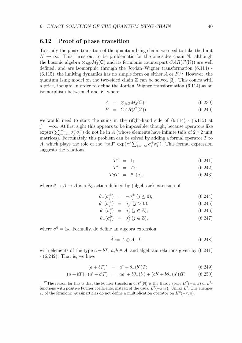
6 EXACT SOLUTION OF THE QUANTUM ISING CHAIN 40
6.12 Proof of phase transition
To study the phase transition of the quantum Ising chain, we need to take the limitN → ∞. This turns out to be problematic for the one-sides chain N: althoughthe bosonic algebra ⊗j∈NM2(C) and its fermionic counterpart CAR(`2(N)) are welldefined, and are isomorphic through the Jordan–Wigner transformation (6.114) -(6.115), the limiting dynamics has no simple form on either A or F .17 However, thequantum Ising model on the two-sided chain Z can be solved [3]. This comes witha price, though: in order to define the Jordan–Wigner transformation (6.114) as anisomorphism between A and F , where
A = ⊗j∈ZM2(C); (6.239)
F = CAR(`2(Z)), (6.240)
we would need to start the sums in the rifght-hand side of (6.114) - (6.115) atj = −∞. At first sight this appears to be impossible, though, because operators likeexp(πi
∑i−1j=−∞ σ
+j σ−j ) do not lie in A (whose elements have infinite tails of 2×2 unit
matrices). Fortunately, this problem can be solved by adding a formal operator T toA, which plays the role of the “tail” exp(πi
∑0j=−∞ σ
+j σ−j ). This formal expression
suggests the relations
T 2 = 1; (6.241)
T ∗ = T ; (6.242)
TaT = θ−(a), (6.243)
where θ− : A→ A is a Z2-action defined by (algebraic) extension of
θ−(σ±j ) = −σ±j (j ≤ 0); (6.244)
θ−(σ±j ) = σ±j (j > 0); (6.245)
θ−(σzj ) = σzj (j ∈ Z); (6.246)
θ−(σ0j ) = σ0
j (j ∈ Z), (6.247)
where σ0 = 12. Formally, de define an algebra extension
A := A⊕ A · T, (6.248)
with elements of the type a+ bT , a, b ∈ A, and algebraic relations given by (6.241)- (6.242). That is, we have
(a+ bT )∗ = a∗ + θ−(b∗)T ; (6.249)
(a+ bT ) · (a′ + b′T ) = aa′ + bθ−(b′) + (ab′ + bθ−(a′))T. (6.250)
17The reason for this is that the Fourier transform of `2(N) is the Hardy space H2(−π, π) of L2-functions with positive Fourier coefficents, instead of the usual L2(−π, π). Unlike L2, The energiesεk of the fermionic quasiparticles do not define a multiplication operator on H2(−π, π).

6 EXACT SOLUTION OF THE QUANTUM ISING CHAIN 41
The correct version of (6.114) - (6.115) may now be written down as
c±i = Te∓πiP0
j=i σ+j σ−j σ±i (i < 1); (6.251)
c±1 = Tσ±1 ; (6.252)
c±i = Te∓πiPi−1
j=1 σ+j σ−j σ±i (i > 1), (6.253)
with formal inverse
σ±i = Te±πiP0
j=i c+j c−j c±i (i < 1); (6.254)
σ±1 = Tc±1 ; (6.255)
σ±i = Te±πiPi−1
j=1 σ+j σ−j σ±i (i > 1), (6.256)
where this time we regard T as an element of the extended fermionic algebra
F := F ⊕ F · T, (6.257)
satisfying the same rules (6.241) - (6.243), but now in terms of a “fermionic” Z2-action θj : F → F given by extending the following action on elementary operators:
θ−(c±j ) = −c±j (j ≤ 0); (6.258)
θ−(c±j ) = c±j (j > 0); (6.259)
θ−(czj) = czj (j ∈ Z); (6.260)
θ−(c0j) = c0
j (j ∈ Z). (6.261)
Because of T , the Jordan–Wigner transformation fails to give an isomorphism A ∼=F , but it does given an isomorphism A ∼= F . More importantly, if, having alreadydefined the Z2-action θ on F by (6.214), we define a similar Z2-action on A by
θ(σ±j ) = −σ±j (j ∈ Z); (6.262)
θ(σzj ) = σzj (j ∈ Z); (6.263)
θ(σ0j ) = σ0
j (j ∈ Z), (6.264)
and grade A and F by the latter, i.e., by θ (see (6.209), and analogously F =F+ ⊕ F−), we have isomorphisms
A+∼= F+; (6.265)
A− ∼= F−T ; (6.266)
A ∼= F+ ⊕ F−T. (6.267)
For given dynamics (6.159), suppose ωA0 is a Z2-invariant ground state on A. ThenωA0 also defines a Z2-invariant ground state ωF0 on F by (6.265) and ωF0 (f) = 0 forall f ∈ F−. Conversely, a Z2-invariant ground state ωF0 on F defines a state ωA0 onA by (6.265) and ωA0 (a) = 0 for all a ∈ A−. But F has a unique ground state, so:
• Either ω0 is pure on A, in which case it is the unique ground state on A;
• Or ω0 is mixed on A, in which case ω0 = 12(ω+
0 + ω−0 ), where ω±0 are pure buttransform under the above Z2-action θ as ω±0 θ = ω∓0 .

6 EXACT SOLUTION OF THE QUANTUM ISING CHAIN 42
Theorem 6.29 gives a representation-theoretical criterion deciding between thesepossibilities, but to apply it we need some information on the restriction of Z2-invariant quasi-free pure states on F to its even part F+ [3]. The abstract settinginvolves a Z2-action W on K that commutes with Γ (so that W is unitary, W 2 = 1,and [Γ,W ] = 0), which induces a Z2-action θ on F by linear and algebraic extensionof θ(Φ(h)) = Φ(Wh). A quasi-free state ωP , defined according to Theorem 6.31 bya projection P : K → K that satisfies (6.234), is then Z2-invariant iff [W,P ] = 0.
In our case, this simplifies to θ(Φ(h)) = −Φ(h), so that W = −1, and everyprojection commutes with W . In any case, we have [2, 5]:
Lemma 6.33 Given some Z2-action W on K, as well as a projection P : K → Ksatisfying (6.234), such that [W,Γ] = [W,P ] = 0:
1. the quasi-free state ωP of Theorem 6.31 is Z2-invariant (i.e., ωP θ = ωP );
2. the corresponding GNS-representation space HP ≡ HωPfor F = F+ ⊕ F−
decomposes as HP = H+P ⊕ H−P , with H±P = F±ΩP . Each subspace H±P is
stable under πP (F+), and the restriction π±P of π(F+) to H±P is irreducible.
Theorem 6.29 then leads to a lemma, which also summarizes the discussion so far.
Lemma 6.34 For given Z2-invariant dynamics, let ωF0 be the (unique, Z2-invariant)ground state on F = F+ ⊕ F−. Under F+ ⊂ F the associated GNS-representationspace H0 decomposes as H0 = H+
0 ⊕ H−0 , with H±0 = F±Ω0, and we denote therestriction of π0(F+) to H±0 by π±0 . Then π±0 (F+) are irreducible.
We regard ωF0 also as a state ωT0 on F+ ⊕ F−T by putting ωT0 (a) = 0 for alla ∈ F−T , and similarly as a state ωA0 on A by invoking (6.265) and putting ωA0 (a) = 0for all a ∈ A−. Let HT
0 = HT+ ⊕HT
− be the GNS-representation space of F+ ⊕ F−Tdefined by ωT0 , where HT
+ = F+Ω and HT− = F−TΩ. Here HT
+ and HT− are stable
under F+; we denote the restriction of F+ to HT± by πT±, so that πT+
∼= π+0 .
1. Then ωA0 is a ground state on A. Any Z2-invariant ground state on A arisesin this way (via F ), so that there is a unique Z2-invariant ground state on A.
2. The state ωA0 is pure on A iff the irreducible representations πT+(F+) (or π+0 (F+))
and πT−(F+) are inequivalent.
It turns out to be difficult to directly check the (in)equivalence of πT±(F+). For-tunately, we can circumvent this problem by passing to yet another (irreducible)representation of F+. We first enlarge F to a new algebra
F = F ⊕ FT = F+ ⊕ F− ⊕ F+T ⊕ F−T, (6.268)
and extend the state ωF0 on F to a state ω0 on F by putting ω0(FT ) = 0, so thatω0 is nonzero only on F+ ⊂ F . Let π0 be the associated GNS-representation of F
on the Hilbert space H0 = F Ω. Under π(F+) this space decomposes as
H0 = F+Ω0 ⊕ F−Ω0 ⊕ F+T Ω0 ⊕ F−T Ω0, (6.269)
with corresponding restrictions π±(F+) and πT±(F+); more precisely, π± is the restric-
tion of π(F+) to F±Ω0, whilst πT± is is the restriction of π(F+) to F±T Ω0. Clearly:

6 EXACT SOLUTION OF THE QUANTUM ISING CHAIN 43
• π±(F+) is the same as π±0 (F+);
• πT−(F+) is just our earlier πT−(F+);
• πT+(F+) has not been encountered before.
To understand the latter, we rewrite (6.269) as
H0 = H0 ⊕ HT0 ; (6.270)
H0 = F+Ω0 ⊕ F−Ω0∼= F+Ω0 ⊕ F−Ω0; (6.271)
HT0 = F+T Ω0 ⊕ F−T Ω0, (6.272)
the point being that π(F ) evidently restricts to both H0 and HT0 . We know the
action of π(F ) on H0 quite well: it is the representation induced by the groundstate ω0. As to HT
0 , we define a state ωT0 on F by
ωT0 (a) := 〈π(T )Ω0, π(a)π(T )Ω0〉H0= 〈Ω0, π(θ−(a))Ω0〉H0
, (6.273)
where the second equality follows from (6.243). Comparing H0 and H0, for all b ∈ F(and hence especially for b = θ−(a)) we simply have
〈Ω0, π(b)Ω0〉H0= ω0(b) = ωF0 (b), (6.274)
so that ωT0 = ωF0 θ− ≡ θ∗−ωF0 . Consequently, if we decompose the GNS-representation
space Hθ∗−ωF0
of πθ∗−ωF0
(F ) as Hθ∗−ωF0
= H+θ∗−ω
F0⊕H−
θ∗−ωF0
, then πT+(F+) is (equivalent to)
the restriction of πθ∗−ωF0
(F+) to H+θ∗−ω
F0
. Therefore, the representation π(F ) restricted
to HT0 is (equivalent to) the GNS-representation πθ∗−ωF
0(F ), so that in turn πT+(F+) is
(equivalent to) πθ∗−ωF0
(F+), restricted to H+θ∗−ω0
. Hence, further to (6.270) - (6.272),
π(F ) ∼= πωF0
(F )⊕ πθ∗−ωF0
(F ). (6.275)
The point is that for the quantum Ising chain Hamiltonian (6.166) we have:
Lemma 6.35 1. For each λ 6= ±1 we have πωF0
(F ) ∼= πθ∗−ωF0
(F ).
2. If this holds, then the representations π+0 (F+) ≡ π+
ωF0
(F+) and πT−(F+) are
inequivalent iff the representations π+ωF
0(F+) and π+
θ∗−ωF0
(F+) are equivalent.
3. For each λ 6= ±1 the ground state ωA0 is pure on A iff the representationsπωF
0(F+) and πθ∗−ωF
0(F+) are equivalent.
The first claim follows the fundamental Theorem 6.37 below. The third follows fromLemma 6.34 and the previous claims.
Exercise 6.36 Prove the second claim by repeatedly applying Theorem 6.29 to π(F ).

6 EXACT SOLUTION OF THE QUANTUM ISING CHAIN 44
Given this lemma, the real issue now lies in comparing πωF0
and πθ∗−ωF0
, both as
representations of F (as they are defined) and as representations of F+ ⊂ F . Thiscan be settled in great generality by first looking at Theorem 6.31 and Exercise 6.32,and thence realizing that
πωF0
= πE+ ; (6.276)
πθ∗−ωF0
= πW−E+W− . (6.277)
Here W− : K → K is the Z2-action on K defining the Z2-action θ− on F asexplained above Lemma 6.33; specifically, W− is the direct sum of two copies ofw− : `2(Z)→ `2(Z), defined by w−(fj) = fj (j > 0) and w−(fj) = −fj (j ≤ 0).
Subsequently, we invoke a basic result on the CAR-algebra [1, 2, 5].
Theorem 6.37 Let P and P ′ be projections on K that satisfy (6.234). Then:
1. πP (F ) ∼= πP ′(F ) iff P − P ′ ∈ B2(K);
2. π+P (F+) ∼= π+
P ′(F+) iff P − P ′ ∈ B2(K) and dim(PK ∩ (1− P ′)K) is even.
Here B2(K) is the class of Hilbert–Schmidt operators on K, which consists of allcompact operators a on K for which
∑i µi < ∞, where the µi are the eigenvalues
of a∗a. ‘Morally’, the first condition indicates that P and P ′ should differ only bya finite-dimensional part, but formally this statement is only literally equivalent tothe states condition if [P, P ′] = 0. In any cae, if the first condition is satisfied, thedimension in the second part is finite, so that one may indeed say it is even or odd.
From Lemmas 6.34 and 6.35 and Theorem 6.37, we finally obtain:
Theorem 6.38 The unique Z2-invariant ground state ω0 of the Hamiltonian (6.166)is pure (and hence forms the unique ground state) iff both of the following hold:
E+ −W−E+W− ∈ B2(K); (6.278)
dim(E+K ∩ (1−W−E+W−)K) is even. (6.279)
This is true for all λ with |λ| ≥ 1. If , on the other hand, |λ| < 1, then ω0 =12(ω+
0 +ω−0 ), where ω±0 are pure and transform under the Z2-action θ as ω±0 θ = ω∓0 .
The computations establishing this final result are formidable, and we refer to [3].

6 EXACT SOLUTION OF THE QUANTUM ISING CHAIN 45
6.13 Classical Ising model in d = 2
6.13.1 Motivation from quantum theory
In general, a quantum lattice model in dimension d at inverse temperature β =(kBT )−1, defined on Λ ⊂ Zd ⊂ Rd, can be mapped into a classical lattice modelin dimension d + 1 on Λ × Λ0, where the additional dimension Λ0 is contained inthe interval [0, β] (this includes the limit β → ∞, in which case thermal averagesgive ground state averages). This mapping becomes exact in the limit where Λ0
approaches [0, β], in that the lattice spacing in Λ0 is taken to be a and one takesthe double limit a → 0, Λ0 → N, with a|Λ0| = β. For example, take the quantumIsing chain (6.124), where d = 1 and Λ = N = 1, . . . , N i.e.,
hN = −JN∑i=1
σzi σzi+1 − Γ
N∑i=1
σxi . (6.280)
Here we take periodic boundary conditions, so that sN+1 ≡ s1. Using the Trotterproduct formula for (noncommuting) matrices A and B, i.e.,
eA+B = limL→∞
(eA/LeB/L
)L, (6.281)
in terms of a = β/L (so that L = |Λ0|) we obtain
Tr e−βhN = limL→∞,a→0,aL=β
Tr((eaΓ
Pi σ
xi eaJ
Pi σ
zi σ
zi+1)L)
, (6.282)
where the trace is taken over the Hilbert space⊗NC2. In each copy of C2 we use basisstates e+ = (1, 0) and e− = (0, 1), so that we can speak of em for m = ±1 ≡ 2,with corresponding basis vectors es = ⊗Ni=1esi
of ⊗NC2, defined by s ∈ 2N , ors : N → 2, or s = (si)
Ni=1 (cf. §1.2.1). Writing es ≡ |s〉 = |s1 · · · sN〉, we have
Tr (TL) =∑
s(1)∈2N ,...,s(L)∈2N
〈s(1)|T |s(2)〉〈s(2)|T |s(3)〉 · · · 〈s(L)|T |s(1)〉, (6.283)
where each |s(j)〉 runs over all basis vectors of ⊗NC2. Using the identity
〈m|eK∗σx|m′〉 =√
sinh(K∗) cosh(K∗)eKmm′, (6.284)
where K and K∗ (which will be K∗ = ha) are related by
K∗ = arctanh(e−2K) ⇔ K = − 12 ln
(eK∗ − e−K∗
eK∗ + e−K∗
), (6.285)
the expression (6.282) becomes
Tr e−βhN = limL→∞,a→0,aL=β
(sinh(ha) cosh(ha))L/2∑
s∈2N×L
ehId=2N,L (s), (6.286)
hId=2N,L (s) =
N∑i=1
L∑j=1
(K(a)si,jsi,j+1 + J(a)si,jsi+1,j) , (6.287)
where K(a) is given as K in (6.285) with K∗ = ha, and J(a) = Ja. This is a certainlimit of the partition function of the classical Ising model in d = 2, with anisotropiccouplings (that is, K(a) 6= J(a)). This motivates a general study of this model.

6 EXACT SOLUTION OF THE QUANTUM ISING CHAIN 46
6.13.2 Hamiltonian, partition function, and transfer matrix
The variables of the classing Ising model in d = 2, defined on a rectangular latticeΛ = N × L, are s ∈ 2N×L, but it is useful to treat each direction differently andregard s as a function s : N → 2L. In other words, we use the canonical isomorphism
2N×L ∼=(2L)N
, (6.288)
given by s(i, j) ≡ si,j ↔ si(j). So from now on, s will be a function N → 2L, andinstead of s(i) we write si ∈ 2L. In terms of these, the Hamiltonian is given by
hId=2N,L (s) =
N∑i=1
(H
(0)N,L(si) +H
(I)N,L(si, si+1)
); (6.289)
H(0)N,L(si) = −J2
L∑j=1
si(j)si(j + 1); (6.290)
H(I)N,L(si, sk) = −J1
L∑j=1
si(j)sk(j). (6.291)
Here the idea is that H(0)N,L incorporates the vertical nearest-neighbour interactions,
which take place within a single column, whereas H(I)N,L takes care if the horizontal
nearest-neighbour interactions, which take place between different columns. In thisway, the model already looks like a one-dimensional Ising model, in which, however,the si take values in 2L rather than in 2. As a case in point, let us recall thatthe transfer matrix T of the classical one-dimensional Ising model (with periodicboundary conditions), with Hamiltonian
hId=1N = −J
N∑i=1
sisi+1, (6.292)
is given (in terms of the usual coupling constant K = βJ) by
T =
(eK e−K
e−K eK
)⇔ T (si, sk) = eKsisk , (6.293)
where we label the matrix entries by si, sk = (±1,±1) instead of i, j = (1, 2). Since
e−βhId=1N =
N∏i=1
T (si, si+1), (6.294)
the partition function is now given by
ZN ≡∑s∈2N
e−βhId=1N = Tr (TN), (6.295)
so that the free energy density is
fβ ≡ −1
βlimN→∞
1
NZN = − 1
βln(λ+), (6.296)
where λ+ is the largest eigenvalue of T (which, by the Perron–Frobenius Theoremof linear algebra, is real and nondegenerate; it comes out as λ+ = eK + e−K).
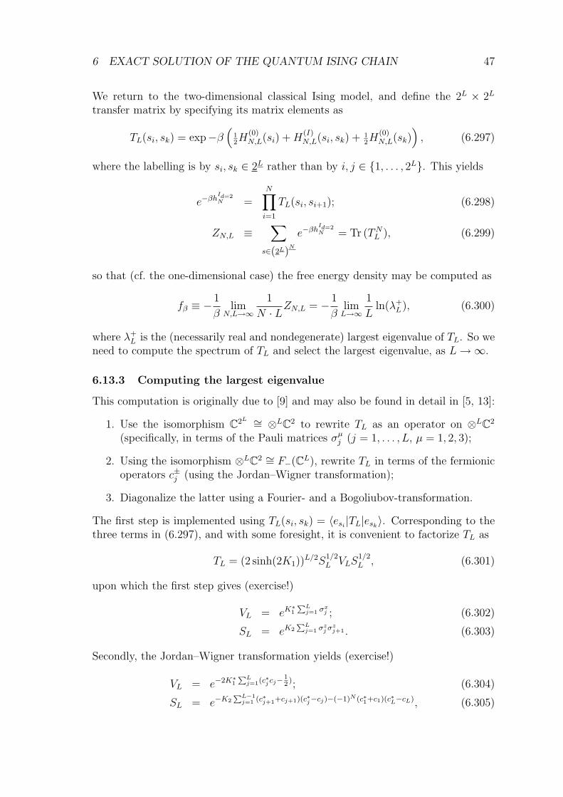
6 EXACT SOLUTION OF THE QUANTUM ISING CHAIN 47
We return to the two-dimensional classical Ising model, and define the 2L × 2L
transfer matrix by specifying its matrix elements as
TL(si, sk) = exp−β(
12H
(0)N,L(si) +H
(I)N,L(si, sk) + 1
2H(0)N,L(sk)
), (6.297)
where the labelling is by si, sk ∈ 2L rather than by i, j ∈ 1, . . . , 2L. This yields
e−βhId=2N =
N∏i=1
TL(si, si+1); (6.298)
ZN,L ≡∑
s∈(2L)N
e−βhId=2N = Tr (TNL ), (6.299)
so that (cf. the one-dimensional case) the free energy density may be computed as
fβ ≡ −1
βlim
N,L→∞
1
N · LZN,L = − 1
βlimL→∞
1
Lln(λ+
L), (6.300)
where λ+L is the (necessarily real and nondegenerate) largest eigenvalue of TL. So we
need to compute the spectrum of TL and select the largest eigenvalue, as L→∞.
6.13.3 Computing the largest eigenvalue
This computation is originally due to [9] and may also be found in detail in [5, 13]:
1. Use the isomorphism C2L ∼= ⊗LC2 to rewrite TL as an operator on ⊗LC2
(specifically, in terms of the Pauli matrices σµj (j = 1, . . . , L, µ = 1, 2, 3);
2. Using the isomorphism ⊗LC2 ∼= F−(CL), rewrite TL in terms of the fermionicoperators c±j (using the Jordan–Wigner transformation);
3. Diagonalize the latter using a Fourier- and a Bogoliubov-transformation.
The first step is implemented using TL(si, sk) = 〈esi|TL|esk
〉. Corresponding to thethree terms in (6.297), and with some foresight, it is convenient to factorize TL as
TL = (2 sinh(2K1))L/2S1/2L VLS
1/2L , (6.301)
upon which the first step gives (exercise!)
VL = eK∗1
PLj=1 σ
xj ; (6.302)
SL = eK2PL
j=1 σzj σ
zj+1 . (6.303)
Secondly, the Jordan–Wigner transformation yields (exercise!)
VL = e−2K∗1PL
j=1(c∗j cj−12 ); (6.304)
SL = e−K2PL−1
j=1 (c∗j+1+cj+1)(c∗j−cj)−(−1)N (c∗1+c1)(c∗L−cL), (6.305)

6 EXACT SOLUTION OF THE QUANTUM ISING CHAIN 48
where the fermion number operator N is given by
N =L∑j=1
c∗jcj. (6.306)
Defining W = −N , we have W ∗ = W and W 2 = 1, so that the fermionic Fock spacedecomposes as F−(CL) = F−(CL)+ ⊕ F−(CL)−, where F−(CL)+/− has an odd/evennumber of occupied states. Since [SL,W ] = 0, also SL = S+
L ⊕ S−L , where
S±L = e−K2PL
j=1(c∗j+1+cj+1)(c∗j−cj), (6.307)
where cL+1 = ±cL. For the plus sign, the Fourier transform is just given by
c(k) =1√L
∑j∈ZL
e−ijkcj, ; (6.308)
cj =1√L
∑k∈ZL
eijkc(k) (6.309)
where ZL = 1, . . . , L (at least initially, see below) is now seen as an abelian groupunder addition modulo L, with dual group,18
ZL = k = 2πn/L, n ∈ ZL. (6.310)
In the limit L → ∞ this yields k ∈ [0, 2π], but (assuming L is even) it is moreconvenient to shift ZL by − 1
2L, so as to have
ZL = − 12L+ 1, . . . , 0, . . . , 1
2L. (6.311)
This time, k takes the values −π+ 2π/L, . . . , 0, . . . , π− 2π/L, π, where each stephas size 2π/L, with limit [−π, π] as L→∞.
For the minus sign in (6.307), the Fourier transform is defined by the sameformulae, but to achieve antiperiodicity cL+1 = −cL, the set ZL ≡ Z+
L is replaced by
Z−L = k = (2n− 1)π/L, n ∈ ZL, (6.312)
so that k ∈ −π + π/L, . . . , π − π/L, again in steps of 2π/L; note that k = 0 doesnot occur. We now isolate the positive parts N±L = Z±L ∩N of Z±L (where N includes
0, so that 0 ∈ Z+L), and for each k in either N+
L\0, π or N−L we define
SL(k) = exp2K2[cos(k)(c∗(k)c(k) + c∗(−k)c(−k)− 1) (6.313)
+i sin(k)(c∗(−k)c∗(k) + c(k)c(−k))]; (6.314)
VL(k) = exp−2K∗1(c∗(k)c(k) + c∗(−k)c(−k)− 1). (6.315)
18The dual group G of a (locally compact) abelian group G consists of the characters on G, i.e.,the one-dimensional representations χ : G → T, where T ⊂ C is the unit circle. As the namesuggest, the dual group is itself a group under (χ · χ′)(g) = χ(g)χ′(g). In our case, G = ZL andeach k ∈ ZL labels a character χk(j) = exp(ijk). In our case, ZL is just a reparametrizationof ZL itself. The Schur orthogonality relations for compact groups then immediately yield usefulrelations like (1/L)
∑Lj=1 exp(ijk) = δk,0 and (1/L)
∑πk=π+2π/L exp(ijk) = δj,0. These, in turn,
give the inversion formula (6.309).

6 EXACT SOLUTION OF THE QUANTUM ISING CHAIN 49
For k = 0 and k = π, however, in order to avoid double counting below, the factors2 above are to be omitted, so that at k = 0 and k = π we have
SL(k) = expK2 · cos(k)(2c∗(k)c(k)− 1); (6.316)
VL(k) = exp−K∗1(2c∗(k)c(k)− 1). (6.317)
The point, then, is this: since also [TL,W ] = 0, we have TL = T+L ⊕ T
−L , with
T±L = (2 sinh(2K1))L/2∏k∈N±L
TL(k); (6.318)
TL(k) = SL(k)1/2VL(k)SL(k)1/2, (6.319)
compare (6.301). Within the product in (6.318), all factors TL(k) mutually commute,so that the set σ(TL) of eigenvalues of TL also decomposes and then factorizes as
σ(TL) = σ(T+L ) ∪ σ(T−L ); (6.320)
σ(T±L ) = (2 sinh(2K1))L/2∏k∈N±L
σ(TL(k)). (6.321)
To compute σ(T±L ), the operators (6.319) need to be diagonalized. As we see from(6.316) - (6.317), for fixed k the operator TL(k) is just a 4×4 matrix for all k exceptk = 0, π, for which it is merely 2 × 2 (namely, each pair of fermion operator c±(k)acts on a two-dimensional space, so that operators involving c±(k) as well as c±(−k)act on a four-dimensional space). A lengthy but straightforward computation, whichmay be accomplished either through the Bogoliubov-transformation mentioned instep 3 above [9, 5], or directly [13] (using a few tricks), yields
∏k∈N+/−
L
σ(TL(k)) =
exp−
∑k∈Z+/−
L
εk(nk − 12)
| nk ∈ 0, 1, ∑k∈Z+/−
L
nk odd/even
,
(6.322)where, for K1 = K2 = K (do the general case yourself!), the ‘energies’ are given by
εk = arccosh(cosh(2(K∗ −K)) + 1− cos(k)), (6.323)
where the sign ambiguity is resolved by the rules [5, 13]
• ε0 = 2(K∗ −K) (which may have either sign, determined by the value of K);
• εk > 0 for all k 6= 0 (so that ε−k = εk).
We have now computed the entire spectrum of TL, but we are really just interestedin the largest eigenvalue λ+
L as L→∞, see (6.300). There are two cases:

6 EXACT SOLUTION OF THE QUANTUM ISING CHAIN 50
1. If ε0 > 0, i.e., if K∗ > K, then the supremum λ+L of the set in (6.322) is
obtained at nk = 0 for all k, which implies that∑
k nk = 0 is even, and hence
ln(λ+L) = 1
2
∑k∈Z−L
εk comes from σ(T−L ). Then
limL→∞
1
Lln(λ+
L) = 12 limL→∞
1
L
∑k∈Z−L
εk =
∫ π
−π
dk
4πεk. (6.324)
2. If ε0 < 0, i.e., if K∗ < K, the supremum lies at n0 = 1, nk = 0 for all k 6= 0,in which case
∑k nk = 1 is odd, and hence ln(λ+
L) = 12(|ε0| +
∑k∈Z+
L\0εk)
comes from σ(T+L ). However, because limk→0 εk = |ε0| (see [5, 13]), the limiting
expression (6.324) is exactly the same for this case.
So in both cases we obtain Onsager’s famous expression for the free energy of theclassical Ising model in d = 2 for K1 = K2 and vanishing external field, viz.
fβ(K) = − 1
2β
(ln(sinh(2K)) +
∫ π
−π
dk
2πεk(K)
). (6.325)
This gives a phase transition at K = K∗, at which point fβ(K)′′ diverges. So thefirst case K∗ > K corresponds to T > Tc, with a unique thermal equilibrium state,whereas in the second case K∗ < K, ot T < Tc, there are two thermal equilibriumstates (this conclusion follows from a detailed analysis of the type given earlier for thequantum model in d = 1, though now classically, see [5]). As a first indication of thisphase structure, note that in the first case supσ(T−L ) as computed above continuesto be above supσ(T+
L ) even as L → ∞, whereas in the second case these supremaasymptotically coincide. Identifying the limits of the corresponding eigenvectors ofTL with equilibrium states then yields the claim. See [5] for a detailed argument.
Exercise 6.39 1. Verify all computations in this chapter.
2. Extend the results to the case K1 6= K2.
3. Extend the results so as to include an external field.

REFERENCES 51
References
[1] H. Araki, Bogoliubov automorphisms and Fock representations of canonicalanticommutation relations, Contemporary Mathematics 62, 23–165 (1987).
[2] H. Araki and D.E. Evans, On a C*-algebra approach to phase transition in thetwo-dimensional Ising model, Commun. Math. Phys. 91, 489–503 (1983).
[3] H. Araki and T. Matsui, Ground states of the XY -model, Commun. Math.Phys. 101, 213–245 (1985).
[4] O. Bratteli and D.W. Robinson, Operator Algebras and Quantum Statisti-cal Mechanics, Vol. ii: Equilibrium States, Models in Statistical Mechanics(Springer, 1981).
[5] D.E. Evans and Y. Kawahigashi, Quantum Symmetries on Operator Algebras(Oxford University Press, 1998).
[6] A. van Enter, R. Fernandez, A. Sokal, J. Stat. Phys. 72, 879–1167 (1993).
[7] H.O. Georgii, Gibbs Measures and Phase Transitions (De Gruyter, 1988).
[8] E. Lieb, T. Schultz, D. Mattis, Two soluble models of an antiferromagneticchain, Ann. Phys. 16, 407–466 (1961).
[9] E. Lieb, T. Schultz, D. Mattis, Two-dimensional Ising model as a soluble prob-lem of many fermions, Rev. Mod. Phys. 36, 856–871 (1964).
[10] P. Pfeuty, The one-dimensional Ising model with a transverse field, Ann. Phys.47, 79–90 (1970).
[11] G. L. Sewell, Quantum Theory of Collective Phenomena (Oxford UniversityPress, 1986).
[12] G. L. Sewell, Quantum Mechanics and its Emergent Macrophysics (PrincetonUniversity Press, 2002).
[13] B. Simon, The Statistical Mechanics of Lattice Gases, Vol. I (Princeton Uni-versity Press, 1993).