Computational Methods

CMSC/AMSC/MAPL 460

Ordinary differential equationsOrdinary differential equations

Ramani Duraiswami,

Dept. of Computer Science

Explicit and One-Step Methods

• Euler Method

• Modified Euler/Midpoint

Up until this point we have dealt with:

• Modified Euler/Midpoint

• Runge-Kutta Methods

These methods are called explicit methods,

because they use only the information from

previous steps.

Moreover these are one-step methods

One Step Method

• These methods allow us to vary the step size.

The one-step techniques

• These methods allow us to vary the step size.

• Use only one initial value.

• After each step is completed the past step is

“forgotten: We do not use this information.

Multi-Step Methods

The principle behind a multi-step method

is to use past values, y and/or dy/dx to

construct a polynomial that approximate construct a polynomial that approximate

the derivative function.

• Represent f(x,y) as a polynomial in x using known values

over the past few steps.

• E.g., using Lagrangian form and equal steps, we have for

3 steps

• (-2h, f-2) (-h, f-1), (0,f0)

• So the polynomial is • So the polynomial is

• f(x)=f-2(x+h)x/(2h2) -f-1(x+2h)x/h2+f0(x+h) (x+2h) /(2h2)

=(x2(f-2+2f-1+f0)+hx(f-2+4f-1+3f0)+2h2f0)/2h2

• Integrate from (xi,xi+1)

Multi-Step Methods

These methods are explicit schemes because the use of

current and past values are used to obtain the future

step.

The method is initiated by using either a set of known

results or from the results of a Runge-Kutta of the same

order to start the initial value problem solution.

Adam Bashforth Method (4 Point)

Example

Consider Exact Solution

2xy

dy−=

x222 exxy −++=

The initial condition is:

The step size is:

2xy

dx

dy−=

22 exxy −++=

( ) 10 =y

0.1h =

4 Point Adam Bashforth

From the 4th order Runge Kutta

( )( )( ) 178597.1218597.1,2.0

094829.1104829.1,1.0

0000.11,0

=

=

=

f

f

f

The 4 Point Adam Bashforth is:

( )( ) 250141.1340141.1,3.0

178597.1218597.1,2.0

=

=

f

f

[ ]01.02.00.3 937595524

1.0 ffffy −+−=∆

4 Point Adam Bashforth

The results are:

( ) ( )( ) ( )19094829.137

178597.159250141.155

24

1.0

−+

−=∆y

Upgrade the values

( ) ( )

( )( ) 308179.1468179.1,4.0

468179.1128038.0340141.14.0

128038.0

19094829.137 24

=

=+=

=

−+

f

y

4 Point Adam Bashforth Method -

Example

The values for the Adam Bashforth

x Adam Bashforth f(x,y) sum 4th order Runge-Kutta Exact

0 1 1 1 1

0.1 1.104828958 1.094829 1.104828958 1.1048290.1 1.104828958 1.094829 1.104828958 1.104829

0.2 1.218596991 1.178597 1.218596991 1.218597

0.3 1.34014081 1.250141 30.72919 1.34014081 1.340141

0.4 1.468179116 1.308179 31.94617 1.468174786 1.468175

0.5 1.601288165 1.351288 32.78612 1.601278076 1.601279

0.6 1.737896991 1.377897 33.20969 1.737880409 1.737881

0.7 1.876270711 1.386271 33.17302 1.876246365 1.876247

0.8 2.014491614 1.374492 32.62766 2.014458009 2.014459

0.9 2.150440205 1.34044 31.52015 2.150395695 2.150397

1 2.281774162 1.281774 29.79136 2.281716852 2.281718

4 Point Adam Bashforth Method -

Example

The explicit Adam

Bashforth method gave

solution gives good

4 Point Adam Bashforth Example

2

4

solution gives good

results without having to

go through large number

of calculations.

-10

-8

-6

-4

-2

0

0 1 2 3 4

X Value

Y V

alu

e

Adam Bashforth

4th order Runge-Kutta

Exact

Deriving the Adams Weights

• Recall that

• The basic idea of an Adams method is to approximate y'(t) in

the above integral by a polynomial Pk(t) of degree k.

• The coefficients of Pk(t) are determined by using the k +1

tdtytytyn

n

t

tnn ∫

+

=−+

1

)()()( ,

1

• The coefficients of Pk(t) are determined by using the k +1

previously calculated data points.

• For example, for P1(t) = At + B, we use (tn-1, yn-1) and (tn, yn),

with P1(tn-1) = f (tn-1, yn-1) = fn-1 and P1(tn) = f (tn, yn) = fn.

• Then

( ) ( )111

11 1,

1−−−

−−−=−=⇒

=+

=+nnnnnn

nn

nntftf

hBff

hA

fBAt

fBAt

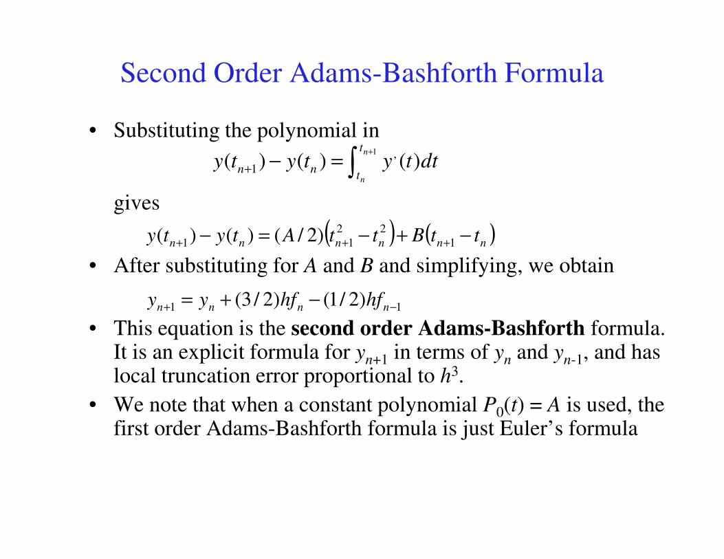
Second Order Adams-Bashforth Formula

• Substituting the polynomial in

gives

• After substituting for A and B and simplifying, we obtain

( ) ( )nnnnnn ttBttAtyty −+−=− +++ 1

22

11 )2/()()(

tdtytytyn

n

t

tnn ∫

+

=−+

1

)()()( ,

1

• This equation is the second order Adams-Bashforth formula. It is an explicit formula for yn+1 in terms of yn and yn-1, and has local truncation error proportional to h3.

• We note that when a constant polynomial P0(t) = A is used, the first order Adams-Bashforth formula is just Euler’s formula

11 )2/1()2/3( −+ −+= nnnn hfhfyy

Fourth Order Adams-Bashforth Formula

• More accurate Adams formulas are obtained by using a higher

degree polynomial Pk(t) and more data points.

• For example, the coefficients of a 3rd degree polynomial P3(t)

are found using (tn, yn), (tn-1, yn-1), (tn-2, yn-2), (tn-3, yn-3).

• As before, P3(t) then replaces y'(t) in the integral equation

nt

∫+

=−1 ,

to obtain the fourth order Adams-Bashforth formula

• The local truncation error of this method is proportional to h5.

( )3211 9375955)24/( −−−+ −+−+= nnnnnn ffffhyy

tdtytytyn

n

t

tnn ∫

+

=−+

1

)()()( ,

1

Stability

• It turns out that explicit methods are not very stable

• This means that the solution may oscillate if we use large

time steps

• So, if we wish to integrate over a large interval, and we

need to take many small steps to achieve accuracy, many

function evaluations are needed.

• Implicit methods are usually more stable

Implicit Methods

• There are second set of multi-step methods, which are

known as “implicit” methods.

– “implicit” => not directly revealed

• Here it means that the value of the function at the later

time is not provided in an “explicit” formula, but in an

equationequation

• Since future data is used an iterative method must be

used to iterate an initial guess to convergence

• Could use Runge-Kutta or Adams Bashforth to start the

initial value problem.

Implicit Multi-Step Methods

The main method is Adams Moulton Method

Three Point Adams-Moulton Method

[ ]i 1 i i 1y 5 812

hf f f+ −∆ = + −

[ ]i 1 i i 1 i 2y 9 19 524

hf f f f+ − −∆ = + − +

Four Point Adams-Moulton Method

Deriving Adams-Moulton Weights

• A variation on the Adams-Bashforth formulas gives another set

of formulas called the Adams-Moulton formulas.

• We begin with the second order case, and use a first degree

polynomial Q1(t) = αt + β to approximate y'(t).

• To determine α and β , we now use (tn, yn) and (tn+1, yn+1):

( ) ( )ft 11=+ βα

• As before, Q1(t) replaces y'(t) in the integral equation to obtain

the second order Adams-Moulton formula

• Note that this equation implicitly defines yn+1. The local

truncation error of this method is proportional to h3.

( ) ( )nnnnnn

nn

nntftf

hff

hft

ft111

11

1,

1+++

++

−=−=⇒

=+

=+βα

βα

βα

( )( ) ( )( )11111 2/),(2/ +++++ ++=++= nnnnnnnnn ffhyytffhyy

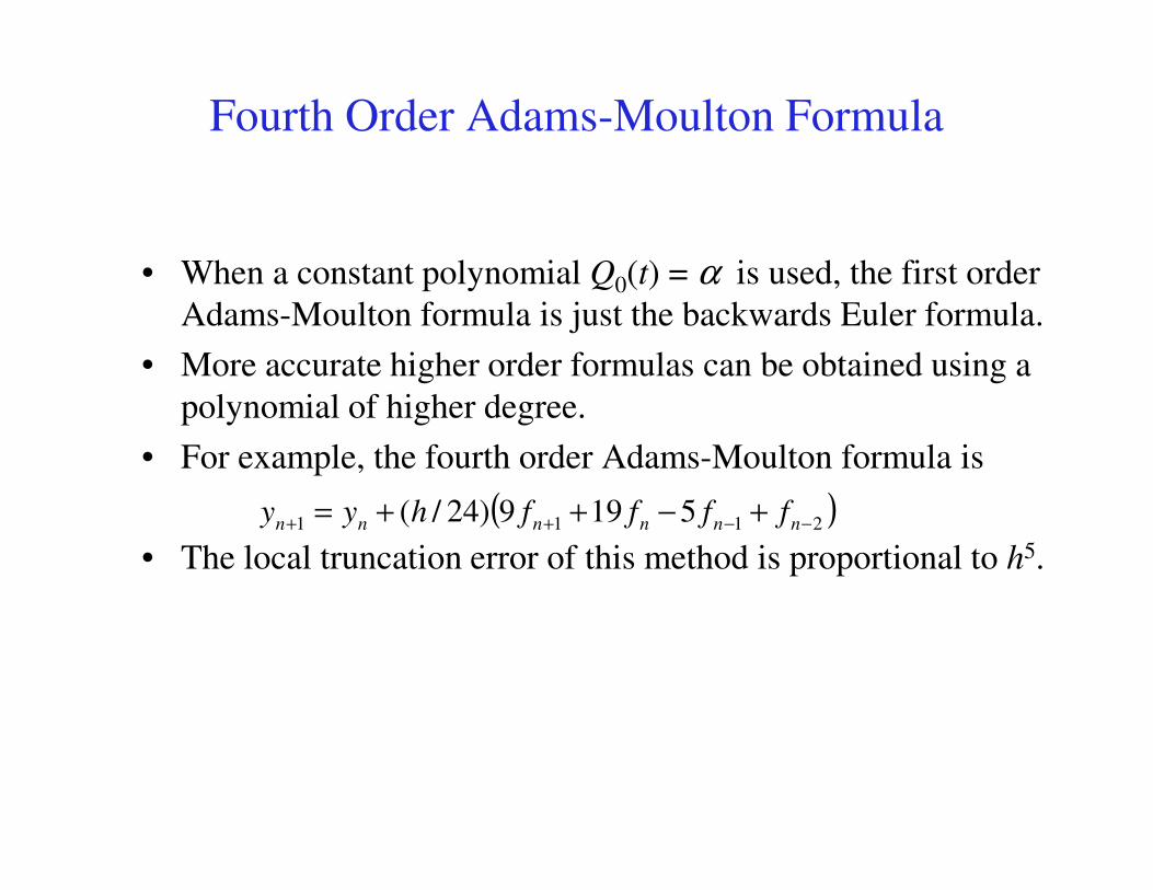
Fourth Order Adams-Moulton Formula

• When a constant polynomial Q0(t) = α is used, the first order

Adams-Moulton formula is just the backwards Euler formula.

• More accurate higher order formulas can be obtained using a

polynomial of higher degree.

• For example, the fourth order Adams-Moulton formula is• For example, the fourth order Adams-Moulton formula is

• The local truncation error of this method is proportional to h5.

( )2111 5199)24/( −−++ +−++= nnnnnn ffffhyy

Implicit Multi-Step Methods

•The method uses what is known as a Predictor-Corrector

technique.

•explicit scheme to estimate the initial guess

•uses the value to guess the future y* and dy/dx= f*(x,y*)•uses the value to guess the future y* and dy/dx= f*(x,y*)

• Using these results, apply Adam Moulton method

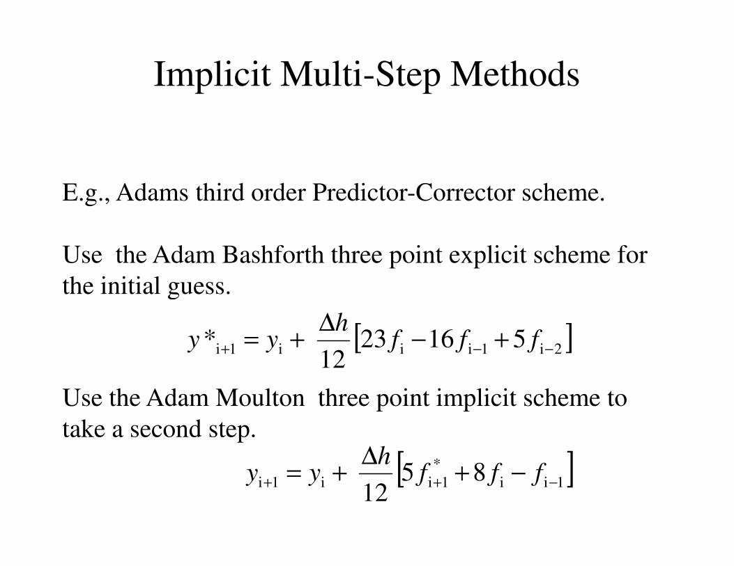
Implicit Multi-Step Methods

E.g., Adams third order Predictor-Corrector scheme.

Use the Adam Bashforth three point explicit scheme for

the initial guess. the initial guess.

Use the Adam Moulton three point implicit scheme to

take a second step.

[ ]2i1iii1i 5162312

* −−+ +−∆

+= fffh

yy

[ ]1ii

*

1ii1i 8512

−++ −+∆

+= fffh

yy

Adam Moulton Method (3 point)

Example

Consider Exact Solution

2xy

dy−=

x222 exxy −++=

The initial condition is:

The step size is:

2xy

dx

dy−=

22 exxy −++=

( ) 10 =y

1.0=∆h

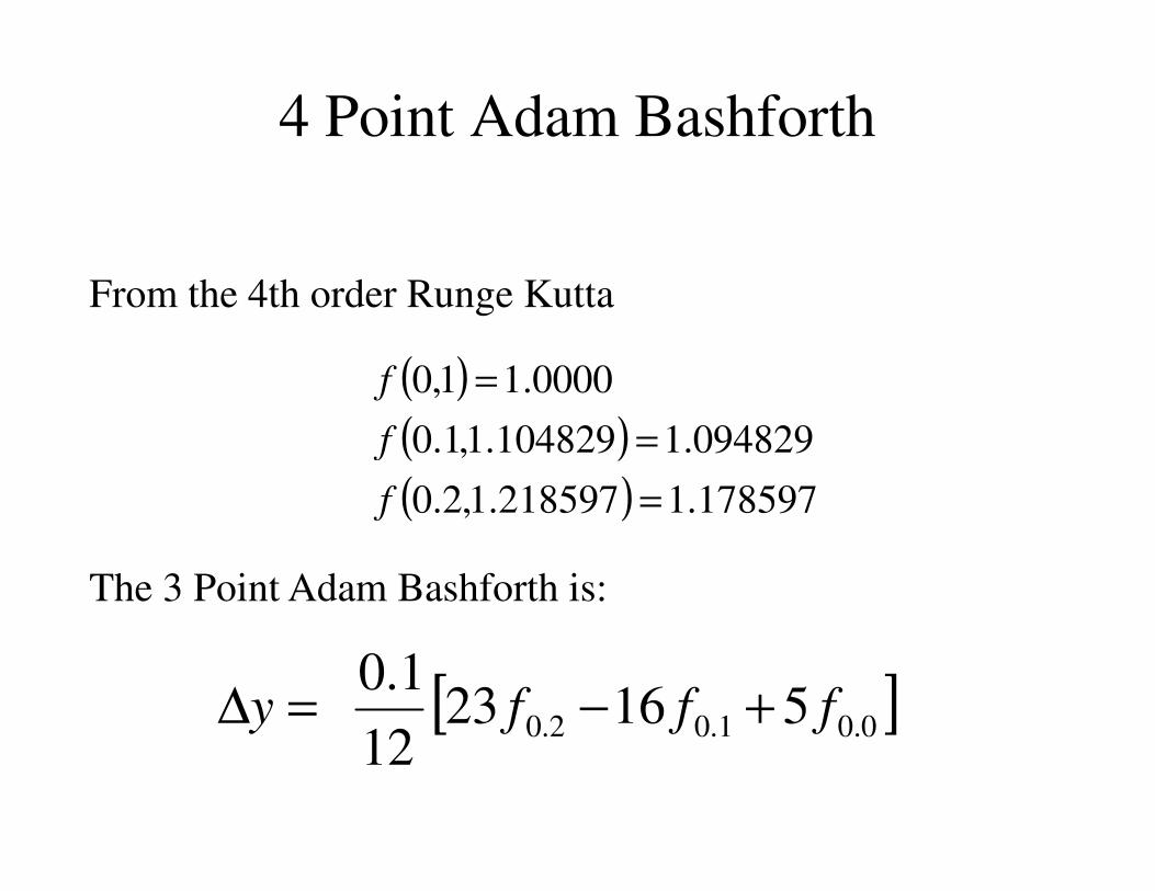
4 Point Adam Bashforth

From the 4th order Runge Kutta

( )( ) 094829.1104829.1,1.0

0000.11,0

=

=

f

f

The 3 Point Adam Bashforth is:

( )( ) 178597.1218597.1,2.0

094829.1104829.1,1.0

=

=

f

f

[ ]0.01.00.2 5162312

1.0 fffy +−=∆

3 Point Adam Moulton

Predictor-Corrector Method

The results of explicit scheme is:

( ) ( ) ( )[ ]15094829.116178597.12312

1.0 +−=∆y

The functional values are:

( )( ) 250184.1340184.1,3.0*

340184.1121587.0218597.13.0*

121587.0

12

=

=+=

=

f

y

3 Point Adam Moulton

Predictor-Corrector Method

The results of implicit scheme is:

( ) ( ) ( )[ ]094829.11178597.18250184.1512

1.0 −+=∆y

The functional values are:

( )( ) 250138.1340184.1,3.0

340138.1121541.0218597.13.0

121541.0

12

=

=+=

=

f

y

3 Point Adam Moulton

Predictor-Corrector Method

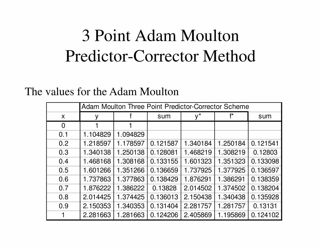
The values for the Adam Moulton

Adam Moulton Three Point Predictor-Corrector Scheme

x y f sum y* f* sum

0 1 10 1 1

0.1 1.104829 1.094829

0.2 1.218597 1.178597 0.121587 1.340184 1.250184 0.121541

0.3 1.340138 1.250138 0.128081 1.468219 1.308219 0.12803

0.4 1.468168 1.308168 0.133155 1.601323 1.351323 0.133098

0.5 1.601266 1.351266 0.136659 1.737925 1.377925 0.136597

0.6 1.737863 1.377863 0.138429 1.876291 1.386291 0.138359

0.7 1.876222 1.386222 0.13828 2.014502 1.374502 0.138204

0.8 2.014425 1.374425 0.136013 2.150438 1.340438 0.135928

0.9 2.150353 1.340353 0.131404 2.281757 1.281757 0.13131

1 2.281663 1.281663 0.124206 2.405869 1.195869 0.124102

3 Point Adam Moulton

Predictor-Corrector Method

The implicit Adam

Moulton method gave

solution gives good

Adam Moulton 3 Point Implicit Scheme

2

4

solution gives good

results without using

more than a three points.

-10

-8

-6

-4

-2

0

2

0 1 2 3 4

X Value

Y V

alu

e4th order Runge-Kutta

Exact

Adam Moulton

Adam Bashforth