lecture_1_s
TRANSCRIPT

7/28/2019 lecture_1_s
http://slidepdf.com/reader/full/lecture1s 1/58
Mathematical Foundation of Electromagnetic Field Theory (MFEFT)
Dr.-Ing. Rene Marklein
FG Electromagnetic TheoryFB 16 Electrical Engineering / Computer Science
University of Kassel
WS 2007/2008
Dr.-Ing. Rene Marklein (University of Kassel) Mathematical Foundation of EFT (MFEFT) WS 2007/2008 1 / 71

7/28/2019 lecture_1_s
http://slidepdf.com/reader/full/lecture1s 2/58

7/28/2019 lecture_1_s
http://slidepdf.com/reader/full/lecture1s 3/58
MFEFT - Outline
1 Introduction
2 Vector and Tensor Algebra
3 Position Vector and Coordinate Systems
4 Vectors: Scalar Product; Vector Product; Dyadic Product
5 Vector and Tensor Analysis
6 Distributions
7 Complex Analysis
8 Special Functions
9 Fourier Transform
10 Laplace Transform
Dr.-Ing. Rene Marklein (University of Kassel) Mathematical Foundation of EFT (MFEFT) WS 2007/2008 3 / 71

7/28/2019 lecture_1_s
http://slidepdf.com/reader/full/lecture1s 4/58
Lecture 1: Introduction; Vector- and Tensor Algebra; Position Vector andCoordinate Systems
Dr.-Ing. Rene Marklein (University of Kassel) Mathematical Foundation of EFT (MFEFT) WS 2007/2008 4 / 71
I d i

7/28/2019 lecture_1_s
http://slidepdf.com/reader/full/lecture1s 5/58
Introduction
MFEFT - Lecture 1
1 Introduction
2
Vector and Tensor Algebra3 Position Vector and Coordinate Systems
Cartesian CoordinatesEinstein’s Summation ConventionDifferentiation of the Position Vector; Kronecker Symbol (Kronecker Delta)Cylinder Coordinate SystemOrthogonal Curvilinear Coordinate SystemSpherical Coordinate SystemDupin Coordinates
4 Vectors: Scalar Product; Vector Product; Dyadic Product
5 Vector and Tensor Analysis
6 Distributions
7 Complex Analysis
8 Special Functions
9 Fourier Transform
10 Laplace Transform
Dr.-Ing. Rene Marklein (University of Kassel) Mathematical Foundation of EFT (MFEFT) WS 2007/2008 5 / 71
Int od ction

7/28/2019 lecture_1_s
http://slidepdf.com/reader/full/lecture1s 6/58
Introduction
Introduction
In the following lecture series we are going to discuss the mathematical basis of electromagnetic fields and waves as solutions of the theory of James Clerk Maxwell
We do not claim completeness!
We provide the essential results and facts without detailed proofs.
We try to provide a sketch of the derivations and explain, illustrate, and discuss themathematical relations.
We follow in principle the first book chapter of the German manuscript by Karl-J org
Langenberg [2002]:
[Langenberg , 2002] K.-J. Langenberg: Theory of Electromagnetic Waves. Manuskript,Universitat Kassel, Kassel, 2002 (in German).
→ You can get a copy of the CD with this Manuscript!Contact: Dr.-Ing. Rene Marklein in his office or wire e-mail: [email protected]
Dr.-Ing. Rene Marklein (University of Kassel) Mathematical Foundation of EFT (MFEFT) WS 2007/2008 6 / 71
Introduction

7/28/2019 lecture_1_s
http://slidepdf.com/reader/full/lecture1s 7/58
Introduction
Introduction
In the following lecture series we are going to discuss the mathematical basis of electromagnetic fields and waves as solutions of the theory of James Clerk Maxwell
We do not claim completeness!
We provide the essential results and facts without detailed proofs.
We try to provide a sketch of the derivations and explain, illustrate, and discuss themathematical relations.
We follow in principle the first book chapter of the German manuscript by Karl-J org
Langenberg [2002]:
[Langenberg , 2002] K.-J. Langenberg: Theory of Electromagnetic Waves. Manuskript,Universitat Kassel, Kassel, 2002 (in German).
→ You can get a copy of the CD with this Manuscript!Contact: Dr.-Ing. Rene Marklein in his office or wire e-mail: [email protected]
Dr.-Ing. Rene Marklein (University of Kassel) Mathematical Foundation of EFT (MFEFT) WS 2007/2008 6 / 71
Introduction

7/28/2019 lecture_1_s
http://slidepdf.com/reader/full/lecture1s 8/58
Introduction
Introduction
In the following lecture series we are going to discuss the mathematical basis of electromagnetic fields and waves as solutions of the theory of James Clerk Maxwell
We do not claim completeness!
We provide the essential results and facts without detailed proofs.
We try to provide a sketch of the derivations and explain, illustrate, and discuss themathematical relations.
We follow in principle the first book chapter of the German manuscript by Karl-J org
Langenberg [2002]:
[Langenberg , 2002] K.-J. Langenberg: Theory of Electromagnetic Waves. Manuskript,Universitat Kassel, Kassel, 2002 (in German).
→ You can get a copy of the CD with this Manuscript!Contact: Dr.-Ing. Rene Marklein in his office or wire e-mail: [email protected]
Dr.-Ing. Rene Marklein (University of Kassel) Mathematical Foundation of EFT (MFEFT) WS 2007/2008 6 / 71
Introduction

7/28/2019 lecture_1_s
http://slidepdf.com/reader/full/lecture1s 9/58
Introduction
Introduction
In the following lecture series we are going to discuss the mathematical basis of electromagnetic fields and waves as solutions of the theory of James Clerk Maxwell
We do not claim completeness!
We provide the essential results and facts without detailed proofs.
We try to provide a sketch of the derivations and explain, illustrate, and discuss themathematical relations.
We follow in principle the first book chapter of the German manuscript by Karl-J org
Langenberg [2002]:
[Langenberg , 2002] K.-J. Langenberg: Theory of Electromagnetic Waves. Manuskript,Universitat Kassel, Kassel, 2002 (in German).
→ You can get a copy of the CD with this Manuscript!Contact: Dr.-Ing. Rene Marklein in his office or wire e-mail: [email protected]
Dr.-Ing. Rene Marklein (University of Kassel) Mathematical Foundation of EFT (MFEFT) WS 2007/2008 6 / 71
Introduction

7/28/2019 lecture_1_s
http://slidepdf.com/reader/full/lecture1s 10/58
Introduction
In the following lecture series we are going to discuss the mathematical basis of electromagnetic fields and waves as solutions of the theory of James Clerk Maxwell
We do not claim completeness!
We provide the essential results and facts without detailed proofs.
We try to provide a sketch of the derivations and explain, illustrate, and discuss themathematical relations.
We follow in principle the first book chapter of the German manuscript by Karl-J org
Langenberg [2002]:
[Langenberg , 2002] K.-J. Langenberg: Theory of Electromagnetic Waves. Manuskript,Universitat Kassel, Kassel, 2002 (in German).
→ You can get a copy of the CD with this Manuscript!Contact: Dr.-Ing. Rene Marklein in his office or wire e-mail: [email protected]
Dr.-Ing. Rene Marklein (University of Kassel) Mathematical Foundation of EFT (MFEFT) WS 2007/2008 6 / 71
Introduction
7/28/2019 lecture_1_s
http://slidepdf.com/reader/full/lecture1s 11/58
Introduction
Our idol is the mathematician Gustav Doetsch, who wrote books for engineers about theFourier and Laplace transform as well as the theory of distributions. We point out the bookchapter [Doetsch, 1967]:
[Doetsch, 1967] G. Doetsch: Funktionaltransformationen . In: R. Sauer, I. Szabo (Eds.):Mathematische Hilfsmittel des Ingenieurs, Teil I . Springer-Verlag, Berlin, 1967.
We are going the follow the books:Vector and Tensor Algebra by Hollis Chen [1983]:
[Chen, 1983] H.C. Chen: Theory of Electromagnetic Waves . McGraw-Hill, New York,1983.
Functional Theory by Heinrich Behnke and Friedrich Sommer [Behnke & Sommer , 1965]:
[Behnke & Sommer , 1965] H. Behnke, F. Sommer: Theorie der analytischen Funktionen
einer komplexen Ver anderlichen. Springer-Verlag, Berlin 1965.Vector and Tensor Analysis by the 4th Volume of the Mathematics for Engineers by K. Burg,
H. Haf und F. Wille (”BHW“) Burg et al.[1990]:
[Burg et al., 1990] K. Burg, H. Haf, F. Wille: H ohere Mathematik f ur Ingenieure, Band
IV: Vektoranalysis und Funktionentheorie . B.G. Teubner, Stuttgart 1990.The main features about Special Functions are derived from the Book Theory of Ordinary
Differential Equations in the Complex Domain by Smirnow [1959]:
[Smirnow
, 1959] W.I. Smirnow:Lehrgang der h¨ ohere n M athematik, Teil III,2
. VEBDeutscher Verlag der Wissenschaften, Berlin 1959.Dr.-Ing. Rene Marklein (University of Kassel) Mathematical Foundation of EFT (MFEFT) WS 2007/2008 7 / 71
Introduction

7/28/2019 lecture_1_s
http://slidepdf.com/reader/full/lecture1s 12/58
Introduction
Our idol is the mathematician Gustav Doetsch, who wrote books for engineers about theFourier and Laplace transform as well as the theory of distributions. We point out the bookchapter [Doetsch, 1967]:
[Doetsch, 1967] G. Doetsch: Funktionaltransformationen . In: R. Sauer, I. Szabo (Eds.):Mathematische Hilfsmittel des Ingenieurs, Teil I . Springer-Verlag, Berlin, 1967.
We are going the follow the books:Vector and Tensor Algebra by Hollis Chen [1983]:
[Chen, 1983] H.C. Chen: Theory of Electromagnetic Waves . McGraw-Hill, New York,1983.
Functional Theory by Heinrich Behnke and Friedrich Sommer [Behnke & Sommer , 1965]:
[Behnke & Sommer , 1965] H. Behnke, F. Sommer: Theorie der analytischen Funktionen
einer komplexen Ver anderlichen. Springer-Verlag, Berlin 1965.Vector and Tensor Analysis by the 4th Volume of the Mathematics for Engineers by K. Burg,
H. Haf und F. Wille (”BHW“) Burg et al.[1990]:
[Burg et al., 1990] K. Burg, H. Haf, F. Wille: H ohere Mathematik f ur Ingenieure, Band
IV: Vektoranalysis und Funktionentheorie . B.G. Teubner, Stuttgart 1990.The main features about Special Functions are derived from the Book Theory of Ordinary
Differential Equations in the Complex Domain by Smirnow [1959]:
[Smirnow , 1959] W.I. Smirnow: Lehrgang der h¨ ohere n M athematik, Teil III,2 . VEBDeutscher Verlag der Wissenschaften, Berlin 1959.
Dr.-Ing. Rene Marklein (University of Kassel) Mathematical Foundation of EFT (MFEFT) WS 2007/2008 7 / 71
Introduction

7/28/2019 lecture_1_s
http://slidepdf.com/reader/full/lecture1s 13/58
Introduction
Our idol is the mathematician Gustav Doetsch, who wrote books for engineers about theFourier and Laplace transform as well as the theory of distributions. We point out the bookchapter [Doetsch, 1967]:
[Doetsch, 1967] G. Doetsch: Funktionaltransformationen . In: R. Sauer, I. Szabo (Eds.):Mathematische Hilfsmittel des Ingenieurs, Teil I . Springer-Verlag, Berlin, 1967.
We are going the follow the books:Vector and Tensor Algebra by Hollis Chen [1983]:
[Chen, 1983] H.C. Chen: Theory of Electromagnetic Waves . McGraw-Hill, New York,1983.
Functional Theory by Heinrich Behnke and Friedrich Sommer [Behnke & Sommer , 1965]:
[Behnke & Sommer , 1965] H. Behnke, F. Sommer: Theorie der analytischen Funktionen
einer komplexen Ver anderlichen. Springer-Verlag, Berlin 1965.Vector and Tensor Analysis by the 4th Volume of the Mathematics for Engineers by K. Burg,
H. Haf und F. Wille (”BHW“) Burg et al.[1990]:
[Burg et al., 1990] K. Burg, H. Haf, F. Wille: H ohere Mathematik f ur Ingenieure, Band
IV: Vektoranalysis und Funktionentheorie . B.G. Teubner, Stuttgart 1990.The main features about Special Functions are derived from the Book Theory of Ordinary
Differential Equations in the Complex Domain by Smirnow [1959]:
[Smirnow , 1959] W.I. Smirnow: Lehrgang der h¨ ohere n M athematik, Teil III,2 . VEBDeutscher Verlag der Wissenschaften, Berlin 1959.
Dr.-Ing. Rene Marklein (University of Kassel) Mathematical Foundation of EFT (MFEFT) WS 2007/2008 7 / 71
Introduction

7/28/2019 lecture_1_s
http://slidepdf.com/reader/full/lecture1s 14/58
Introduction
Our idol is the mathematician Gustav Doetsch, who wrote books for engineers about theFourier and Laplace transform as well as the theory of distributions. We point out the bookchapter [Doetsch, 1967]:
[Doetsch, 1967] G. Doetsch: Funktionaltransformationen . In: R. Sauer, I. Szabo (Eds.):Mathematische Hilfsmittel des Ingenieurs, Teil I . Springer-Verlag, Berlin, 1967.
We are going the follow the books:Vector and Tensor Algebra by Hollis Chen [1983]:
[Chen, 1983] H.C. Chen: Theory of Electromagnetic Waves . McGraw-Hill, New York,1983.
Functional Theory by Heinrich Behnke and Friedrich Sommer [Behnke & Sommer , 1965]:
[Behnke & Sommer , 1965] H. Behnke, F. Sommer: Theorie der analytischen Funktionen
einer komplexen Ver anderlichen. Springer-Verlag, Berlin 1965.Vector and Tensor Analysis by the 4th Volume of the Mathematics for Engineers by K. Burg,
H. Haf und F. Wille (”BHW“) Burg et al.[1990]:
[Burg et al., 1990] K. Burg, H. Haf, F. Wille: H ohere Mathematik f ur Ingenieure, Band
IV: Vektoranalysis und Funktionentheorie . B.G. Teubner, Stuttgart 1990.The main features about Special Functions are derived from the Book Theory of Ordinary
Differential Equations in the Complex Domain by Smirnow [1959]:
[Smirnow , 1959] W.I. Smirnow: Lehrgang der h¨ ohere n M athematik, Teil III,2 . VEBDeutscher Verlag der Wissenschaften, Berlin 1959.
Dr.-Ing. Rene Marklein (University of Kassel) Mathematical Foundation of EFT (MFEFT) WS 2007/2008 7 / 71
Introduction

7/28/2019 lecture_1_s
http://slidepdf.com/reader/full/lecture1s 15/58
Introduction
Our idol is the mathematician Gustav Doetsch, who wrote books for engineers about theFourier and Laplace transform as well as the theory of distributions. We point out the bookchapter [Doetsch, 1967]:
[Doetsch, 1967] G. Doetsch: Funktionaltransformationen . In: R. Sauer, I. Szabo (Eds.):Mathematische Hilfsmittel des Ingenieurs, Teil I . Springer-Verlag, Berlin, 1967.
We are going the follow the books:Vector and Tensor Algebra by Hollis Chen [1983]:
[Chen, 1983] H.C. Chen: Theory of Electromagnetic Waves . McGraw-Hill, New York,1983.
Functional Theory by Heinrich Behnke and Friedrich Sommer [Behnke & Sommer , 1965]:
[Behnke & Sommer , 1965] H. Behnke, F. Sommer: Theorie der analytischen Funktionen
einer komplexen Ver anderlichen. Springer-Verlag, Berlin 1965.Vector and Tensor Analysis by the 4th Volume of the Mathematics for Engineers by K. Burg,
H. Haf und F. Wille (”BHW“) Burg et al.[1990]:
[Burg et al., 1990] K. Burg, H. Haf, F. Wille: H ohere Mathematik f ur Ingenieure, Band
IV: Vektoranalysis und Funktionentheorie . B.G. Teubner, Stuttgart 1990.The main features about Special Functions are derived from the Book Theory of Ordinary
Differential Equations in the Complex Domain by Smirnow [1959]:
[Smirnow , 1959] W.I. Smirnow: Lehrgang der h¨ ohere n M athematik, Teil III,2 . VEBDeutscher Verlag der Wissenschaften, Berlin 1959.
Dr.-Ing. Rene Marklein (University of Kassel) Mathematical Foundation of EFT (MFEFT) WS 2007/2008 7 / 71
Introduction

7/28/2019 lecture_1_s
http://slidepdf.com/reader/full/lecture1s 16/58
Introduction
Our idol is the mathematician Gustav Doetsch, who wrote books for engineers about theFourier and Laplace transform as well as the theory of distributions. We point out the bookchapter [Doetsch, 1967]:
[Doetsch, 1967] G. Doetsch: Funktionaltransformationen . In: R. Sauer, I. Szabo (Eds.):Mathematische Hilfsmittel des Ingenieurs, Teil I . Springer-Verlag, Berlin, 1967.
We are going the follow the books:Vector and Tensor Algebra by Hollis Chen [1983]:
[Chen, 1983] H.C. Chen: Theory of Electromagnetic Waves . McGraw-Hill, New York,1983.
Functional Theory by Heinrich Behnke and Friedrich Sommer [Behnke & Sommer , 1965]:
[Behnke & Sommer , 1965] H. Behnke, F. Sommer: Theorie der analytischen Funktionen
einer komplexen Ver anderlichen. Springer-Verlag, Berlin 1965.Vector and Tensor Analysis by the 4th Volume of the Mathematics for Engineers by K. Burg,
H. Haf und F. Wille (”BHW“) Burg et al.[1990]:
[Burg et al., 1990] K. Burg, H. Haf, F. Wille: H ohere Mathematik f ur Ingenieure, Band
IV: Vektoranalysis und Funktionentheorie . B.G. Teubner, Stuttgart 1990.The main features about Special Functions are derived from the Book Theory of Ordinary
Differential Equations in the Complex Domain by Smirnow [1959]:
[Smirnow , 1959] W.I. Smirnow: Lehrgang der h¨ ohere n M athematik, Teil III,2 . VEBDeutscher Verlag der Wissenschaften, Berlin 1959.
Dr.-Ing. Rene Marklein (University of Kassel) Mathematical Foundation of EFT (MFEFT) WS 2007/2008 7 / 71
Vector and Tensor Algebra

7/28/2019 lecture_1_s
http://slidepdf.com/reader/full/lecture1s 17/58
MFEFT - Lecture 1
1 Introduction
2 Vector and Tensor Algebra
3 Position Vector and Coordinate SystemsCartesian CoordinatesEinstein’s Summation ConventionDifferentiation of the Position Vector; Kronecker Symbol (Kronecker Delta)Cylinder Coordinate SystemOrthogonal Curvilinear Coordinate System
Spherical Coordinate SystemDupin Coordinates
4 Vectors: Scalar Product; Vector Product; Dyadic Product
5 Vector and Tensor Analysis
6 Distributions
7 Complex Analysis
8 Special Functions
9 Fourier Transform
10 Laplace Transform
Dr.-Ing. Rene Marklein (University of Kassel) Mathematical Foundation of EFT (MFEFT) WS 2007/2008 8 / 71
Vector and Tensor Algebra

7/28/2019 lecture_1_s
http://slidepdf.com/reader/full/lecture1s 18/58
Electromagnetic Fields
Electromagnetic Fields; Vector Fields; Maxwell’s Equations
Electromagnetic Fields are Vector Fields, which are a function of Time t and thethree-dimensional Position Vector R; Maxwell’s Equations
∇×E(R, t) = −∂ B(R, t)
∂t− J
m(R, t)
∇×H(R, t) =∂ D(R, t)
∂t+ J
e(R, t)
∇·D(R, t) = e(R, t)
∇·B(R, t) = m(R, t)
describing the Physics of their interaction through the change in Time and Space, this requiresMathematical Tools to describe such changes of Vector Fields and their Algebraic Interrelation.
Dr.-Ing. Rene Marklein (University of Kassel) Mathematical Foundation of EFT (MFEFT) WS 2007/2008 9 / 71
Vector and Tensor Algebra

7/28/2019 lecture_1_s
http://slidepdf.com/reader/full/lecture1s 19/58
Electromagnetic Fields
Electromagnetic Fields; Vector Fields; Maxwell’s Equations
Electromagnetic Fields are Vector Fields, which are a function of Time t and thethree-dimensional Position Vector R; Maxwell’s Equations
∇×E(R, t) = −∂ B(R, t)
∂t− J
m(R, t)
∇×H(R, t) =∂ D(R, t)
∂t+ J
e(R, t)
∇·D(R, t) = e(R, t)
∇·B(R, t) = m(R, t)
describing the Physics of their interaction through the change in Time and Space, this requiresMathematical Tools to describe such changes of Vector Fields and their Algebraic Interrelation.
Dr.-Ing. Rene Marklein (University of Kassel) Mathematical Foundation of EFT (MFEFT) WS 2007/2008 9 / 71
Vector and Tensor Algebra

7/28/2019 lecture_1_s
http://slidepdf.com/reader/full/lecture1s 20/58
Literature
Further literature of the topic vector/tensor algebra and analysis
[Tai , 1992] C. T. Tai: Generalized Vector and Dyadic Analysis. IEEE Press, New York 1992
[Bourne & Kendall , 1988] D. E. Bourne, P. C. Kendall: Vektoranalysis . TeubnerStudienbucher, B. G. Teubner, Stuttgart 1988
[Teichmann, 1963] H. Teichmann: Physikalische Anwendungen der Vektor- und Tensorrechnung . Bibliographisches Institut, Mannheim 1963
[Fetzer , 1978] V. Fetzer: Mathematik f ur Elektrotechniker, Band 1. Huthig Verlag,Heidelberg 1978
[Spiegel , 1977] M. S. Spiegel: Vektoranalysis . Schaum’s Outline, McGraw-Hill, Hamburg,
1977.[Morse & Feshbach, 1953] P. M. Morse, H. Feshbach: Methods of Theoretical Physics, Part
I and Part II. McGraw-Hill, New York, 1953.
Dr.-Ing. Rene Marklein (University of Kassel) Mathematical Foundation of EFT (MFEFT) WS 2007/2008 10 / 71
Position Vector and Coordinate Systems Cartesian Coordinates

7/28/2019 lecture_1_s
http://slidepdf.com/reader/full/lecture1s 21/58
MFEFT - Lecture 1
1 Introduction
2 Vector and Tensor Algebra
3 Position Vector and Coordinate SystemsCartesian CoordinatesEinstein’s Summation ConventionDifferentiation of the Position Vector; Kronecker Symbol (Kronecker Delta)Cylinder Coordinate SystemOrthogonal Curvilinear Coordinate System
Spherical Coordinate SystemDupin Coordinates
4 Vectors: Scalar Product; Vector Product; Dyadic Product
5 Vector and Tensor Analysis
6 Distributions
7 Complex Analysis
8 Special Functions
9 Fourier Transform
10 Laplace Transform
Dr.-Ing. Rene Marklein (University of Kassel) Mathematical Foundation of EFT (MFEFT) WS 2007/2008 11 / 71
Position Vector and Coordinate Systems Cartesian Coordinates

7/28/2019 lecture_1_s
http://slidepdf.com/reader/full/lecture1s 22/58
Cartesian Coordinate SystemCartesian Coordinates; Unit Vectors, Magnitude of the Position Vector
x , y, z Coordinate Axes like Heinrich Hertz:
”Wir nehmen an, dass das benutzte
Coordinatensystem der x , y, z von solcher
Beschaffenheit ist, dass, wenn die Richtung der
positiven x von uns aus nach vorn, die der positiven
z von uns aus nach oben geht, alsdann die y von
links nach rechts hin wachsen.“
English translation:”
We assume that the used coordinate system of x , y, z is in such a way, that, if
the direction of the positive x points from us to the
front, the positive z points from us upwards, and yincreases from left to right“.
[Hertz , 1890] H. R. Hertz: Uber die
Grundgleichungen der Elektrodynamik f urruhende Korper. Nachrichten von der
K oniglichen Gesellschaft der Wissenschaften
und der Georg-August-Universit at zu
G ottingen, pp. 106-149; nachgedruckt inAnnalen der Physik , Vol. 40, pp. 577-624,1890.
Cartesian Coordinates of the spatialpoint P and the related positionvector
.........
.........
.........
.........
.........
.........
.........
.........
.........
..........................
.........
.........
.........
.........
.........
.........
.........
.................
................
............................................................................................................................................................... ....................................................................................................................................................
.....................
O
x
y
z
Dr.-Ing. Rene Marklein (University of Kassel) Mathematical Foundation of EFT (MFEFT) WS 2007/2008 12 / 71
Position Vector and Coordinate Systems Cartesian Coordinates

7/28/2019 lecture_1_s
http://slidepdf.com/reader/full/lecture1s 23/58
Cartesian Coordinate SystemCartesian Coordinates; Unit Vectors, Magnitude of the Position Vector
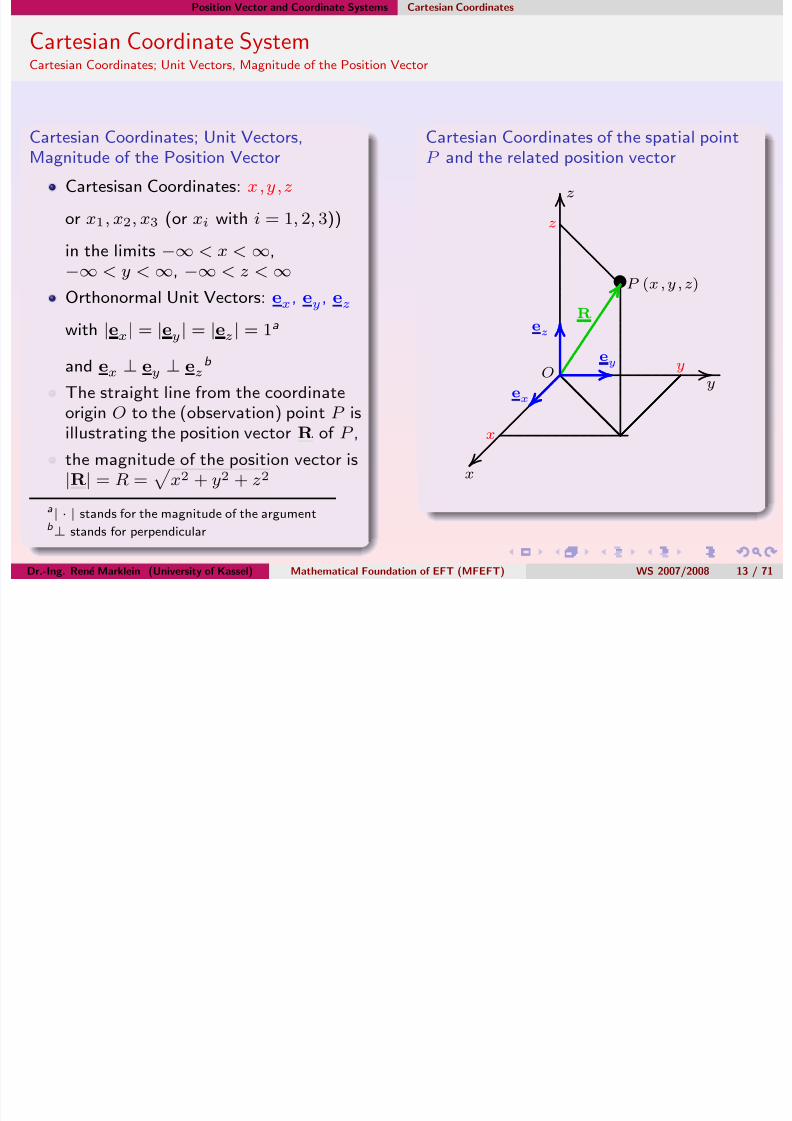
Cartesian Coordinates; Unit Vectors,Magnitude of the Position Vector
Cartesisan Coordinates: x , y, z
or x1, x2, x3 (or xi with i = 1, 2, 3))
in the limits −∞ < x < ∞,
−∞ < y < ∞, −∞ < z < ∞Orthonormal Unit Vectors: ex, ey , ez
with |ex| = |ey | = |ez | = 1a
and ex ⊥ ey ⊥ ezb
The straight line from the coordinate
origin O to the (observation) point P isillustrating the position vector R of P ,
the magnitude of the position vector is|R| = R =
x2 + y2 + z2
a| · | stands for the magnitude of the argumentb ⊥ stands for perpendicular
Cartesian Coordinates of the spatial pointP and the related position vector
.........
.........
.........
.........
.........
.........
.........
.........
.........
.........
.........
.....................
.........
.........
.........
.........
.........
.........
.........
.........
.........
.........
....................
................
.................................................................................................................................................................................................. .................................................................................................................................................................................
......................
.............................................................................................................................................................................................
..........................
..........................
.......................................................................................................................
.................................................................................................................................................
..................................................................................................................................................................................................................................................
.......................................
..........................
..................
u
..
..
..
..
..
..
..
..
..
..
..
..
..
..
..
..
..
..
..
..
..
..
..
..
..
..
..
..
..
..
..
..
..
..
..
..
..
..
..
..
..
..
..
..
..
..
..
..
..
..
..
..
.........................................................
..
..
..
..
..
..
..
..
..
..
..
..
..
..
..
..
..
..
..
..
..
..
..
..
..
..
..
..
..
..
.................
................
.............................................................................
................
...................................................................
................
O
x
y
z
z
x
y
P (x,y,z)
Rez
ex
ey
Dr.-Ing. Rene Marklein (University of Kassel) Mathematical Foundation of EFT (MFEFT) WS 2007/2008 13 / 71
Position Vector and Coordinate Systems Cartesian Coordinates
7/28/2019 lecture_1_s
http://slidepdf.com/reader/full/lecture1s 24/58
Cartesian Coordinate SystemCartesian Coordinates; Unit Vectors, Magnitude of the Position Vector
Cartesian Coordinates; Unit Vectors,Magnitude of the Position Vector
Cartesisan Coordinates: x , y, z
or x1, x2, x3 (or xi with i = 1, 2, 3))
in the limits −∞ < x < ∞,
−∞ < y < ∞, −∞ < z < ∞Orthonormal Unit Vectors: ex, ey , ez
with |ex| = |ey | = |ez | = 1a
and ex ⊥ ey ⊥ ezb
The straight line from the coordinate
origin O to the (observation) point P isillustrating the position vector R of P ,
the magnitude of the position vector is|R| = R =
x2 + y2 + z2
a| · | stands for the magnitude of the argumentb ⊥ stands for perpendicular
Cartesian Coordinates of the spatial pointP and the related position vector
.........
.........
.........
.........
.........
.........
.........
.........
.........
.........
.........
....................
.........
.........
.........
.........
.........
.........
.........
.........
.........
.........
.....................
................
.................................................................................................................................................................................................. .................................................................................................................................................................................
......................
............................................................................................................................................................................................
.......................................
.............................................................................
......................................................................................
....................................................................................................................
.................................................................................................................................................................................................................................................
.......................................
..........................
..................
u
..
..
..
..
..
..
..
..
..
..
..
..
..
..
..
..
..
..
..
..
..
..
..
..
..
..
..
..
..
..
..
..
..
..
..
..
..
..
..
..
..
..
..
..
..
..
..
..
..
..
..
..
.........................................................
..
..
..
..
..
..
..
..
..
..
..
..
..
..
..
..
..
..
..
..
..
..
..
..
..
..
..
..
..
..
.................
................
.............................................................................
................
...................................................................
................
O
x
y
z
z
x
y
P (x,y,z)
Rez
ex
ey
Dr.-Ing. Rene Marklein (University of Kassel) Mathematical Foundation of EFT (MFEFT) WS 2007/2008 13 / 71
Position Vector and Coordinate Systems Cartesian Coordinates
C i C di S

7/28/2019 lecture_1_s
http://slidepdf.com/reader/full/lecture1s 25/58
Cartesian Coordinate SystemCartesian Coordinates; Unit Vectors, Magnitude of the Position Vector
Cartesian Coordinates; Unit Vectors,Magnitude of the Position Vector
Cartesisan Coordinates: x , y, z
or x1, x2, x3 (or xi with i = 1, 2, 3))
in the limits −∞ < x < ∞,
−∞ < y < ∞, −∞ < z < ∞Orthonormal Unit Vectors: ex, ey , ez
with |ex| = |ey | = |ez | = 1a
and ex ⊥ ey ⊥ ezb
The straight line from the coordinate
origin O to the (observation) point P isillustrating the position vector R of P ,
the magnitude of the position vector is|R| = R =
x2 + y2 + z2
a| · | stands for the magnitude of the argumentb ⊥ stands for perpendicular
Cartesian Coordinates of the spatial pointP and the related position vector
.........
.........
.........
.........
.........
.........
.........
.........
.........
.........
.........
....................
.........
.........
.........
.........
.........
.........
.........
.........
.........
.........
.....................
................
.................................................................................................................................................................................................. .................................................................................................................................................................................
......................
...........................................................................................................................................................................................
..........................
..........................
.........................................................................................................................
...................................................................................................................................................
...............................................................................................................................................................................................................................................
..........................
.......................................
...................
u
..
..
..
..
..
..
..
..
..
..
..
..
..
..
..
..
..
..
..
..
..
..
..
..
..
..
..
..
..
..
..
..
..
..
..
..
..
..
..
..
..
..
..
..
..
..
..
..
..
..
..
..
.........................................................
..
..
..
..
..
..
..
..
..
..
..
..
..
..
..
..
..
..
..
..
..
..
..
..
..
..
..
..
..
..
.................
................
.............................................................................
................
...................................................................
................
O
x
y
z
z
x
y
P (x,y,z)
Rez
ex
ey
Dr.-Ing. Rene Marklein (University of Kassel) Mathematical Foundation of EFT (MFEFT) WS 2007/2008 13 / 71
Position Vector and Coordinate Systems Cartesian Coordinates
C i C di S

7/28/2019 lecture_1_s
http://slidepdf.com/reader/full/lecture1s 26/58
Cartesian Coordinate SystemCartesian Coordinates; Unit Vectors, Magnitude of the Position Vector
Cartesian Coordinates; Unit Vectors,Magnitude of the Position Vector
Cartesisan Coordinates: x , y, z
or x1, x2, x3 (or xi with i = 1, 2, 3))
in the limits −∞ < x < ∞,
−∞ < y < ∞, −∞ < z < ∞Orthonormal Unit Vectors: ex, ey , ez
with |ex| = |ey | = |ez | = 1a
and ex ⊥ ey ⊥ ezb
The straight line from the coordinate
origin O to the (observation) point P isillustrating the position vector R of P ,
the magnitude of the position vector is|R| = R =
x2 + y2 + z2
a| · | stands for the magnitude of the argumentb ⊥ stands for perpendicular
Cartesian Coordinates of the spatial pointP and the related position vector
.........
.........
.........
.........
.........
.........
.........
.........
.........
.........
.........
...................
.........
.........
.........
.........
.........
.........
.........
.........
.........
.........
......................
................
.................................................................................................................................................................................................. .................................................................................................................................................................................
......................
...........................................................................................................................................................................................
..........................
..........................
.........................................................................................................................
...................................................................................................................................................
...............................................................................................................................................................................................................................................
..........................
.......................................
...................
u
..
..
..
..
..
..
..
..
..
..
..
..
..
..
..
..
..
..
..
..
..
..
..
..
..
..
..
..
..
..
..
..
..
..
..
..
..
..
..
..
..
..
..
..
..
..
..
..
..
..
..
..
.........................................................
..
..
..
..
..
..
..
..
..
..
..
..
..
..
..
..
..
..
..
..
..
..
..
..
..
..
..
..
..
..
.................
................
.............................................................................
................
...................................................................
................
O
x
y
z
z
x
y
P (x,y,z)
Rez
ex
ey
Dr.-Ing. Rene Marklein (University of Kassel) Mathematical Foundation of EFT (MFEFT) WS 2007/2008 13 / 71
Position Vector and Coordinate Systems Cartesian Coordinates
S l d V t i l (V t )C t

7/28/2019 lecture_1_s
http://slidepdf.com/reader/full/lecture1s 27/58
Scalar and Vectorial (Vector)Components
Scalar (Vector)ComponentsThe projections of the vector onto the orthonormal unit vectors ex, ey, ez yield the Scalar(Vector)Components Rx, Ry , Rz of R:
Rx = ex ·R (1)
Ry = ey ·R (2)
Rz = ez ·R (3)
Vectorial (Vector)Components
If we multiply the scalar (vector)components with the relating unit vectors, we obtain theVectorial (Vector)Components Rx, Ry , Rz of R:
Rx = Rx ex = (ex ·R)ex (4)
Ry = Ry ey = (ey ·R) ey (5)
Rz = Rz ez = (ez ·R)ez (6)
Dr.-Ing. Rene Marklein (University of Kassel) Mathematical Foundation of EFT (MFEFT) WS 2007/2008 14 / 71
Position Vector and Coordinate Systems Cartesian Coordinates
S l d V t i l (V t )C t

7/28/2019 lecture_1_s
http://slidepdf.com/reader/full/lecture1s 28/58
Scalar and Vectorial (Vector)Components
Scalar (Vector)ComponentsThe projections of the vector onto the orthonormal unit vectors ex, ey, ez yield the Scalar(Vector)Components Rx, Ry , Rz of R:
Rx = ex ·R (1)
Ry = ey ·R (2)
Rz = ez ·R (3)
Vectorial (Vector)Components
If we multiply the scalar (vector)components with the relating unit vectors, we obtain theVectorial (Vector)Components Rx, Ry , Rz of R:
Rx = Rx ex = (ex ·R)ex (4)
Ry = Ry ey = (ey ·R) ey (5)
Rz = Rz ez = (ez ·R)ez (6)
Dr.-Ing. Rene Marklein (University of Kassel) Mathematical Foundation of EFT (MFEFT) WS 2007/2008 14 / 71
Position Vector and Coordinate Systems Cartesian Coordinates
Scalar and Vectorial (Vector)Components

7/28/2019 lecture_1_s
http://slidepdf.com/reader/full/lecture1s 29/58
Scalar and Vectorial (Vector)Components
Scalar (Vector)ComponentsThe projections of the vector onto the orthonormal unit vectors ex, ey, ez yield the Scalar(Vector)Components Rx, Ry , Rz of R:
Rx = ex ·R (1)
Ry = ey ·R (2)
Rz = ez ·R (3)
Vectorial (Vector)Components
If we multiply the scalar (vector)components with the relating unit vectors, we obtain theVectorial (Vector)Components Rx, Ry , Rz of R:
Rx = Rx ex = (ex ·R)ex (4)
Ry = Ry ey = (ey ·R) ey (5)
Rz = Rz ez = (ez ·R)ez (6)
Dr.-Ing. Rene Marklein (University of Kassel) Mathematical Foundation of EFT (MFEFT) WS 2007/2008 14 / 71
Position Vector and Coordinate Systems Cartesian Coordinates
Scalar and Vectorial (Vector)Components

7/28/2019 lecture_1_s
http://slidepdf.com/reader/full/lecture1s 30/58
Scalar and Vectorial (Vector)Components
Scalar (Vector)ComponentsThe projections of the vector onto the orthonormal unit vectors ex, ey, ez yield the Scalar(Vector)Components Rx, Ry , Rz of R:
Rx = ex ·R (1)
Ry = ey ·R (2)
Rz = ez ·R (3)
Vectorial (Vector)Components
If we multiply the scalar (vector)components with the relating unit vectors, we obtain theVectorial (Vector)Components Rx, Ry , Rz of R:
Rx = Rx ex = (ex ·R)ex (4)
Ry = Ry ey = (ey ·R) ey (5)
Rz = Rz ez = (ez ·R)ez (6)
Dr.-Ing. Rene Marklein (University of Kassel) Mathematical Foundation of EFT (MFEFT) WS 2007/2008 14 / 71
Position Vector and Coordinate Systems Cartesian Coordinates
Cartesian Coordinate System
7/28/2019 lecture_1_s
http://slidepdf.com/reader/full/lecture1s 31/58
Cartesian Coordinate SystemComponent Representation of the Position Vector in the Cartesian Coordinate System
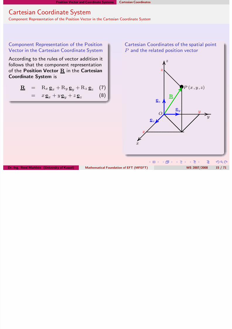
Component Representation of the PositionVector in the Cartesian Coordinate System
According to the rules of vector addition itfollows that the component representationof the Position Vector R in the CartesianCoordinate System is
R = Rx ex + Ry ey + Rz ez (7)
= x ex + y ey + z ez (8)
Cartesian Coordinates of the spatial pointP and the related position vector
.........
.........
.........
.........
.........
.........
.........
.........
.........
.........
.........
.........
.........................
.........
.........
.........
.........
.........
.........
.........
.........
.........................
................
.................................................................................................................................................................................................. .................................................................................................................................................................................
......................
...........................................................................................................................................................................
.................................................
.................................................................
............................................................................................................................
..............................................................................
.......................................................................................................................................................................................................................................................................................
..........................
..........................
............
u
..
..
..
..
..
..
..
..
..
..
..
..
..
..
..
..
..
..
..
..
..
..
..
..
..
..
..
..
..
..
..
..
..
..
..
..
..
..
..
..
..
..
..
..
..
..
..
..
..
..
..
..
..
..
..
..
..
..
..
..
.........................
................
..
..
..
..
..
..
..
..
..
..
..
..
..
..
..
..
..
..
..
..
..
..
..
..
..
..
..
..
..
..
.................
................
.............................................................................
................
............................................
.............
..
..
..
..
..
..........
......
O
x
y
z
z
x
y
P (x,y,z)
Rez
ex
ey
Dr.-Ing. Rene Marklein (University of Kassel) Mathematical Foundation of EFT (MFEFT) WS 2007/2008 15 / 71
Position Vector and Coordinate Systems Cartesian Coordinates
Cartesian Coordinate System

7/28/2019 lecture_1_s
http://slidepdf.com/reader/full/lecture1s 32/58
Cartesian Coordinate SystemComponent Representation of the Position Vector in the Cartesian Coordinate System
Component Representation of the PositionVector in the Cartesian Coordinate System
Using the coordinates x1, x2, x3 it followsfor the Position Vector R in the CartesianCoordinate System
R = xex
+ y ey
+ z ez (9)
= x1 ex1 + x2 ex2 + x3 ex3 (10)
The advantage of this notation is that wecan write the position vector in form of asum:
R = x1 ex1 + x2 ex2 + x3 ex3 (11)
=3
i=1
xi exi(12)
Cartesian Coordinates of the spatial Point P and the related Position Vector R
.........
.........
.........
.........
.........
.........
.........
.........
.........
.........
.........
.........
.........
......................
.........
.........
.........
.........
.........
.........
.........
.........
...................
................
.................................................................................................................................................................................................. .................................................................................................................................................................................
......................
...........................................................................................................................................................................
............................................
..............................................................
............................................................................................................................................
..............................................................
.......................................................................................................................................................................................................................................................................................................
.......................................
.................
u
..
..
..
..
..
..
..
..
..
..
..
..
..
..
..
..
..
..
..
..
..
..
..
..
..
..
..
..
..
..
..
..
..
..
..
..
..
..
..
..
..
..
..
..
..
..
..
..
..
..
..
..
..
..
..
..
..
..
..
..
..
..
..
..
.................
................
..
..
..
..
..
..
..
..
..
..
..
..
..
..
..
..
..
..
..
..
..
..
..
..
..
..
..
..
..
..
.................
................
.............................................................................
................
....................................
...........................
..
..
................
O
x = x1
y = x2
z = x3
x = x1
y = x2
z = x3
P (x,y,z)
= P (x1, x2, x3)R
ez= e
x3
ex = ex1
ey= e
x2
Dr.-Ing. Rene Marklein (University of Kassel) Mathematical Foundation of EFT (MFEFT) WS 2007/2008 16 / 71
Position Vector and Coordinate Systems Einstein’s Summation Convention
Einstein’s Summation Convention

7/28/2019 lecture_1_s
http://slidepdf.com/reader/full/lecture1s 33/58
Einstein s Summation Convention
Einstein’s Summation Convention
The numbered form of Eq. (10) allows a short hand notation using Einstein’s summationconvention:
R =
3i=1
xi exi (13)
def = xi exi
, (14)
i. e., one can delete the sum sign and say:If an index appears only on one side of an equation and more than two times, we have to build a
sum from 1 to 3.
Dr.-Ing. Rene Marklein (University of Kassel) Mathematical Foundation of EFT (MFEFT) WS 2007/2008 17 / 71
Position Vector and Coordinate Systems Einstein’s Summation Convention
Einstein’s Summation Convention

7/28/2019 lecture_1_s
http://slidepdf.com/reader/full/lecture1s 34/58
Einstein s Summation Convention
Einstein’s Summation Convention
The numbered form of Eq. (10) allows a short hand notation using Einstein’s summationconvention:
R =
3i=1
xi exi (13)
def = xi exi
, (14)
i. e., one can delete the sum sign and say:If an index appears only on one side of an equation and more than two times, we have to build a
sum from 1 to 3.
Dr.-Ing. Rene Marklein (University of Kassel) Mathematical Foundation of EFT (MFEFT) WS 2007/2008 17 / 71
Position Vector and Coordinate Systems Einstein’s Summation Convention
Einstein’s Summation Convention

7/28/2019 lecture_1_s
http://slidepdf.com/reader/full/lecture1s 35/58
Einstein s Summation Convention
Einstein’s Summation Convention
The numbered form of Eq. (10) allows a short hand notation using Einstein’s summationconvention:
R =
3i=1
xi exi (13)
def = xi exi
, (14)
i. e., one can delete the sum sign and say:If an index appears only on one side of an equation and more than two times, we have to build a
sum from 1 to 3.
Dr.-Ing. Rene Marklein (University of Kassel) Mathematical Foundation of EFT (MFEFT) WS 2007/2008 17 / 71
Position Vector and Coordinate Systems Differentiation of the Position Vector; Kronecker Symbol (Kronecker Delta)
Differentiation of the Position Vector

7/28/2019 lecture_1_s
http://slidepdf.com/reader/full/lecture1s 36/58
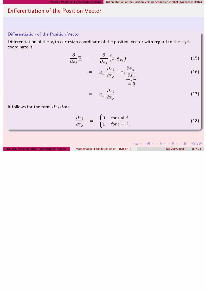
Differentiation of the Position Vector
Differentiation of the xith cartesian coordinate of the position vector with regard to the xjthcoordinate is
∂
∂xj
R =∂
∂xj
xi exi
(15)
=exi
∂xi
∂xj + xi
∂ exi
∂xj = 0
(16)
= exi
∂xi
∂xj
. (17)
It follows for the term ∂xi/∂xj :
∂xi
∂xj
=
0 for i = j
1 for i = j .(18)
Dr.-Ing. Rene Marklein (University of Kassel) Mathematical Foundation of EFT (MFEFT) WS 2007/2008 18 / 71
Position Vector and Coordinate Systems Differentiation of the Position Vector; Kronecker Symbol (Kronecker Delta)
Differentiation of the Position Vector

7/28/2019 lecture_1_s
http://slidepdf.com/reader/full/lecture1s 37/58
Differentiation of the Position Vector
Differentiation of the xith cartesian coordinate of the position vector with regard to the xjthcoordinate is
∂
∂xj
R =∂
∂xj
xi exi
(15)
=exi
∂xi
∂xj + xi
∂ exi
∂xj = 0
(16)
= exi
∂xi
∂xj
. (17)
It follows for the term ∂xi/∂xj :
∂xi
∂xj
=
0 for i = j
1 for i = j .(18)
Dr.-Ing. Rene Marklein (University of Kassel) Mathematical Foundation of EFT (MFEFT) WS 2007/2008 18 / 71
Position Vector and Coordinate Systems Differentiation of the Position Vector; Kronecker Symbol (Kronecker Delta)
Differentiation of the Position Vector

7/28/2019 lecture_1_s
http://slidepdf.com/reader/full/lecture1s 38/58
Differentiation of the Position Vector
Differentiation of the xith cartesian coordinate of the position vector with regard to the xjthcoordinate is
∂
∂xj
R =∂
∂xj
xi exi
(15)
=exi
∂xi
∂xj + xi
∂ exi
∂xj = 0
(16)
= exi
∂xi
∂xj
. (17)
It follows for the term∂x
i/∂x
j :
∂xi
∂xj
=
0 for i = j
1 for i = j .(18)
Dr.-Ing. Rene Marklein (University of Kassel) Mathematical Foundation of EFT (MFEFT) WS 2007/2008 18 / 71
Position Vector and Coordinate Systems Differentiation of the Position Vector; Kronecker Symbol (Kronecker Delta)
Differentiation of the Position Vector
7/28/2019 lecture_1_s
http://slidepdf.com/reader/full/lecture1s 39/58
Differentiation of the Position Vector
Differentiation of the xith cartesian coordinate of the position vector with regard to the xjthcoordinate is
∂
∂xj
R =∂
∂xj
xi exi
(15)
=exi
∂xi
∂xj + xi
∂ exi
∂xj = 0
(16)
= exi
∂xi
∂xj
. (17)
It follows for the term ∂xi
/∂xj
:
∂xi
∂xj
=
0 for i = j
1 for i = j .(18)
Dr.-Ing. Rene Marklein (University of Kassel) Mathematical Foundation of EFT (MFEFT) WS 2007/2008 18 / 71
Position Vector and Coordinate Systems Differentiation of the Position Vector; Kronecker Symbol (Kronecker Delta)
Cartesian Coordinate System

7/28/2019 lecture_1_s
http://slidepdf.com/reader/full/lecture1s 40/58
Differentiation of the Position Vector; Kronecker Symbol (Kronecker Delta)
Differentiation of the Position Vector; Kronecker Symbol (Kronecker Delta)The right-hand side (RSH) of the last Eq. (18) is representing the properties of the KroneckerSymbol (Kronecker Delta):
δij =
0 for i = j
1 for i = j(19)
It follows for the above mentioned differentiation of the position vector with regard to the xjthcoordinate
∂
∂xj
R =∂
∂xj
(xiexi) (20)
=exi
∂xi
∂xj = δij
(21)
= exiδij . (22)
Dr.-Ing. Rene Marklein (University of Kassel) Mathematical Foundation of EFT (MFEFT) WS 2007/2008 19 / 71
Position Vector and Coordinate Systems Differentiation of the Position Vector; Kronecker Symbol (Kronecker Delta)
Cartesian Coordinate System

7/28/2019 lecture_1_s
http://slidepdf.com/reader/full/lecture1s 41/58
Differentiation of the Position Vector; Kronecker Symbol (Kronecker Delta)
Differentiation of the Position Vector; Kronecker Symbol (Kronecker Delta)The right-hand side (RSH) of the last Eq. (18) is representing the properties of the KroneckerSymbol (Kronecker Delta):
δij =
0 for i = j
1 for i = j(19)
It follows for the above mentioned differentiation of the position vector with regard to the xjthcoordinate
∂
∂xj
R =∂
∂xj
(xiexi) (20)
=exi
∂xi
∂xj = δij
(21)
= exiδij . (22)
Dr.-Ing. Rene Marklein (University of Kassel) Mathematical Foundation of EFT (MFEFT) WS 2007/2008 19 / 71
Position Vector and Coordinate Systems Differentiation of the Position Vector; Kronecker Symbol (Kronecker Delta)
Cartesian Coordinate System

7/28/2019 lecture_1_s
http://slidepdf.com/reader/full/lecture1s 42/58
Differentiation of the Position Vector; Kronecker Symbol (Kronecker Delta)
Differentiation of the Position Vector; Kronecker Symbol (Kronecker Delta)The right-hand side (RSH) of the last Eq. (18) is representing the properties of the KroneckerSymbol (Kronecker Delta):
δij =
0 for i = j
1 for i = j(19)
It follows for the above mentioned differentiation of the position vector with regard to the xjthcoordinate
∂
∂xj
R =∂
∂xj
(xiexi) (20)
=exi
∂xi
∂xj = δij
(21)
= exiδij . (22)
Dr.-Ing. Rene Marklein (University of Kassel) Mathematical Foundation of EFT (MFEFT) WS 2007/2008 19 / 71
Position Vector and Coordinate Systems Differentiation of the Position Vector; Kronecker Symbol (Kronecker Delta)
Cartesian Coordinate SystemS ( )

7/28/2019 lecture_1_s
http://slidepdf.com/reader/full/lecture1s 43/58
Differentiation of the Position Vector; Kronecker Symbol (Kronecker Delta)
Differentiation of the Position Vector; Kronecker Symbol (Kronecker Delta)The right-hand side (RSH) of the last Eq. (18) is representing the properties of the KroneckerSymbol (Kronecker Delta):
δij =
0 for i = j
1 for i = j(19)
It follows for the above mentioned differentiation of the position vector with regard to the xjthcoordinate
∂
∂xj
R =∂
∂xj
(xiexi) (20)
= exi
∂xi
∂xj = δij
(21)
= exiδij . (22)
Dr.-Ing. Rene Marklein (University of Kassel) Mathematical Foundation of EFT (MFEFT) WS 2007/2008 19 / 71
Position Vector and Coordinate Systems Differentiation of the Position Vector; Kronecker Symbol (Kronecker Delta)
Cartesian Coordinate SystemDiff i i f h P i i V K k S b l

7/28/2019 lecture_1_s
http://slidepdf.com/reader/full/lecture1s 44/58
Differentiation of the Position Vector; Kronecker Symbol
Differentiation of the Position Vector in Cartesian Coordinates; Kronecker SymbolThe term exi
δij can be simplified to
exiδij
j=i= exi
(23)
or (24)
i=j= exj , (25)
i. e., one can either replace i by j or j by i, because δij is only for i = j unequal of null. We findfor i = j:
∂
∂xj
R = exiδij (26)
i=j= exj
δij (27)
= exj. (28)
Dr.-Ing. Rene Marklein (University of Kassel) Mathematical Foundation of EFT (MFEFT) WS 2007/2008 20 / 71
Position Vector and Coordinate Systems Differentiation of the Position Vector; Kronecker Symbol (Kronecker Delta)
Cartesian Coordinate SystemDiff ti ti f th P iti V t K k S b l

7/28/2019 lecture_1_s
http://slidepdf.com/reader/full/lecture1s 45/58
Differentiation of the Position Vector; Kronecker Symbol
Differentiation of the Position Vector in Cartesian Coordinates; Kronecker SymbolThe term exi
δij can be simplified to
exiδij
j=i= exi
(23)
or (24)
i=j
= exj , (25)
i. e., one can either replace i by j or j by i, because δij is only for i = j unequal of null. We findfor i = j:
∂
∂xj
R = exiδij (26)
i=j= exj
δij (27)
= exj. (28)
Dr.-Ing. Rene Marklein (University of Kassel) Mathematical Foundation of EFT (MFEFT) WS 2007/2008 20 / 71
Position Vector and Coordinate Systems Differentiation of the Position Vector; Kronecker Symbol (Kronecker Delta)
Cartesian Coordinate SystemDifferentiation of the Position Vector; Kronecker Symbol

7/28/2019 lecture_1_s
http://slidepdf.com/reader/full/lecture1s 46/58
Differentiation of the Position Vector; Kronecker Symbol
Differentiation of the Position Vector in Cartesian Coordinates; Kronecker SymbolThe term exi
δij can be simplified to
exiδij
j=i= exi
(23)
or (24)
i=j
= exj , (25)
i. e., one can either replace i by j or j by i, because δij is only for i = j unequal of null. We findfor i = j:
∂
∂xj
R = exiδij (26)
i=j= exj
δij (27)
= exj. (28)
Dr.-Ing. Rene Marklein (University of Kassel) Mathematical Foundation of EFT (MFEFT) WS 2007/2008 20 / 71
Position Vector and Coordinate Systems Differentiation of the Position Vector; Kronecker Symbol (Kronecker Delta)
Cartesian Coordinate SystemDifferentiation of the Position Vector; Kronecker Symbol

7/28/2019 lecture_1_s
http://slidepdf.com/reader/full/lecture1s 47/58
Differentiation of the Position Vector; Kronecker Symbol
Differentiation of the Position Vector in Cartesian Coordinates; Kronecker SymbolThe term exi
δij can be simplified to
exiδij
j=i= exi
(23)
or (24)
i=j
= exj , (25)
i. e., one can either replace i by j or j by i, because δij is only for i = j unequal of null. We findfor i = j:
∂
∂xj
R = exiδij (26)
i=j= exj
δij (27)
= exj. (28)
Dr.-Ing. Rene Marklein (University of Kassel) Mathematical Foundation of EFT (MFEFT) WS 2007/2008 20 / 71
Position Vector and Coordinate Systems Differentiation of the Position Vector; Kronecker Symbol (Kronecker Delta)
Cartesian Coordinate SystemDifferentiation of the Position Vector; Kronecker Symbol

7/28/2019 lecture_1_s
http://slidepdf.com/reader/full/lecture1s 48/58
Differentiation of the Position Vector; Kronecker Symbol
Differentiation of the Position Vector in Cartesian Coordinates; Kronecker SymbolThe term exi
δij can be simplified to
exiδij
j=i= exi
(23)
or (24)
i=j
= exj , (25)
i. e., one can either replace i by j or j by i, because δij is only for i = j unequal of null. We findfor i = j:
∂
∂xj
R = exiδij (26)
i=j= exj
δij (27)
= exj. (28)
Dr.-Ing. Rene Marklein (University of Kassel) Mathematical Foundation of EFT (MFEFT) WS 2007/2008 20 / 71
Position Vector and Coordinate Systems Differentiation of the Position Vector; Kronecker Symbol (Kronecker Delta)
Cartesian Coordinate SystemDifferentiation of the Position Vector; Kronecker Symbol

7/28/2019 lecture_1_s
http://slidepdf.com/reader/full/lecture1s 49/58
Differentiation of the Position Vector; Kronecker Symbol
Differentiation of the Position Vector in Cartesian Coordinates; Kronecker SymbolThe term exi
δij can be simplified to
exiδij
j=i= exi
(23)
or (24)
i=j
= exj , (25)
i. e., one can either replace i by j or j by i, because δij is only for i = j unequal of null. We findfor i = j:
∂
∂xj
R = exiδij (26)
i=j= exj
δij (27)
= exj. (28)
Dr.-Ing. Rene Marklein (University of Kassel) Mathematical Foundation of EFT (MFEFT) WS 2007/2008 20 / 71
Position Vector and Coordinate Systems Differentiation of the Position Vector; Kronecker Symbol (Kronecker Delta)
Cartesian Coordinate SystemDifferentiation of the Position Vector; Kronecker Symbol

7/28/2019 lecture_1_s
http://slidepdf.com/reader/full/lecture1s 50/58
; y
Differentiation of the Position Vector in Cartesian Coordinates; Kronecker SymbolThe term exi
δij can be simplified to
exiδij
j=i= exi
(23)
or (24)
i=j
= exj , (25)
i. e., one can either replace i by j or j by i, because δij is only for i = j unequal of null. We findfor i = j:
∂
∂xj
R = exiδij (26)
i=j= exj
δij (27)
= exj. (28)
Dr.-Ing. Rene Marklein (University of Kassel) Mathematical Foundation of EFT (MFEFT) WS 2007/2008 20 / 71
Position Vector and Coordinate Systems Differentiation of the Position Vector; Kronecker Symbol (Kronecker Delta)
Cartesian Coordinate SystemDifferentiation of the Position Vector; Kronecker Symbol

7/28/2019 lecture_1_s
http://slidepdf.com/reader/full/lecture1s 51/58
Keep in Mind!
Obviously, we obtain the three orthogonal unit vector exj
, j = 1, 2, 3 by differentiating the
position vector with regard to the cartesian coordinate xj :
∂
∂xj
R = exj. (29)
Example (Differentiation of the Position Vector; Kronecker Symbol)
If xjj=1= x1 = x it follows:
With the application of the summation con-vention:
∂
∂x1
R =∂
∂x1(xi exi
) (30)
= exi
∂xi
∂x1 = δi1
(31)
= exiδi1 (32)
= ex1. (33)
Without the summation convention:
∂
∂xR =
∂
∂x x ex + y ey + z ez
(34)
= ∂ ∂x
x = 1
ex + ∂ ∂x
y = 0
ey + ∂ ∂x
z = 0
ez
(35)
= ex . (36)
Dr.-Ing. Rene Marklein (University of Kassel) Mathematical Foundation of EFT (MFEFT) WS 2007/2008 21 / 71
Position Vector and Coordinate Systems Differentiation of the Position Vector; Kronecker Symbol (Kronecker Delta)
Cartesian Coordinate SystemDifferentiation of the Position Vector; Kronecker Symbol

7/28/2019 lecture_1_s
http://slidepdf.com/reader/full/lecture1s 52/58
Keep in Mind!
Obviously, we obtain the three orthogonal unit vector exj
, j = 1, 2, 3 by differentiating the
position vector with regard to the cartesian coordinate xj :
∂
∂xj
R = exj. (29)
Example (Differentiation of the Position Vector; Kronecker Symbol)
If xjj=1= x1 = x it follows:
With the application of the summation con-vention:
∂
∂x1
R =∂
∂x1(xi exi
) (30)
= exi
∂xi
∂x1 = δi1
(31)
= exiδi1 (32)
= ex1. (33)
Without the summation convention:
∂
∂xR =
∂
∂x x ex + y ey + z ez
(34)
= ∂ ∂x
x = 1
ex + ∂ ∂x
y = 0
ey + ∂ ∂x
z = 0
ez
(35)
= ex . (36)
Dr.-Ing. Rene Marklein (University of Kassel) Mathematical Foundation of EFT (MFEFT) WS 2007/2008 21 / 71
Position Vector and Coordinate Systems Differentiation of the Position Vector; Kronecker Symbol (Kronecker Delta)
Cartesian Coordinate SystemDifferentiation of the Position Vector; Kronecker Symbol

7/28/2019 lecture_1_s
http://slidepdf.com/reader/full/lecture1s 53/58
Keep in Mind!
Obviously, we obtain the three orthogonal unit vector exj
, j = 1, 2, 3 by differentiating the
position vector with regard to the cartesian coordinate xj :
∂
∂xj
R = exj. (29)
Example (Differentiation of the Position Vector; Kronecker Symbol)
If xjj=1= x1 = x it follows:
With the application of the summation con-vention:
∂
∂x1
R =∂
∂x1(xi exi
) (30)
= exi
∂xi
∂x1 = δi1
(31)
= exiδi1 (32)
= ex1. (33)
Without the summation convention:
∂
∂xR =
∂
∂x x ex + y ey + z ez
(34)
= ∂ ∂x
x = 1
ex + ∂ ∂x
y = 0
ey + ∂ ∂x
z = 0
ez
(35)
= ex . (36)
Dr.-Ing. Rene Marklein (University of Kassel) Mathematical Foundation of EFT (MFEFT) WS 2007/2008 21 / 71
Position Vector and Coordinate Systems Differentiation of the Position Vector; Kronecker Symbol (Kronecker Delta)
Cartesian Coordinate SystemDifferentiation of the Position Vector; Kronecker Symbol

7/28/2019 lecture_1_s
http://slidepdf.com/reader/full/lecture1s 54/58
Keep in Mind!
Obviously, we obtain the three orthogonal unit vector exj
, j = 1, 2, 3 by differentiating the
position vector with regard to the cartesian coordinate xj :
∂
∂xj
R = exj. (29)
Example (Differentiation of the Position Vector; Kronecker Symbol)
If xjj=1= x1 = x it follows:
With the application of the summation con-vention:
∂
∂x1
R =∂
∂x1(xi exi
) (30)
= exi
∂xi
∂x1 = δi1
(31)
= exiδi1 (32)
= ex1. (33)
Without the summation convention:
∂
∂xR =
∂
∂x x ex + y ey + z ez
(34)
= ∂ ∂x
x = 1
ex + ∂ ∂x
y = 0
ey + ∂ ∂x
z = 0
ez
(35)
= ex . (36)
Dr.-Ing. Rene Marklein (University of Kassel) Mathematical Foundation of EFT (MFEFT) WS 2007/2008 21 / 71
Position Vector and Coordinate Systems Differentiation of the Position Vector; Kronecker Symbol (Kronecker Delta)
Cartesian Coordinate SystemDifferentiation of the Position Vector; Kronecker Symbol

7/28/2019 lecture_1_s
http://slidepdf.com/reader/full/lecture1s 55/58
Keep in Mind!
Obviously, we obtain the three orthogonal unit vector exj
, j = 1, 2, 3 by differentiating the
position vector with regard to the cartesian coordinate xj :
∂
∂xj
R = exj. (29)
Example (Differentiation of the Position Vector; Kronecker Symbol)
If xjj=1= x1 = x it follows:
With the application of the summation con-vention:
∂
∂x1
R =∂
∂x1(xi exi
) (30)
= exi
∂xi
∂x1 = δi1
(31)
= exiδi1 (32)
= ex1. (33)
Without the summation convention:
∂
∂xR =
∂
∂x x ex + y ey + z ez
(34)
= ∂ ∂x
x = 1
ex + ∂ ∂x
y = 0
ey + ∂ ∂x
z = 0
ez
(35)
= ex . (36)
Dr.-Ing. Rene Marklein (University of Kassel) Mathematical Foundation of EFT (MFEFT) WS 2007/2008 21 / 71
Position Vector and Coordinate Systems Differentiation of the Position Vector; Kronecker Symbol (Kronecker Delta)
Cartesian Coordinate SystemDifferentiation of the Position Vector; Kronecker Symbol

7/28/2019 lecture_1_s
http://slidepdf.com/reader/full/lecture1s 56/58
Keep in Mind!
Obviously, we obtain the three orthogonal unit vector exj
, j = 1, 2, 3 by differentiating the
position vector with regard to the cartesian coordinate xj :
∂
∂xj
R = exj. (29)
Example (Differentiation of the Position Vector; Kronecker Symbol)
If xjj=1= x1 = x it follows:
With the application of the summation con-vention:
∂
∂x1
R =∂
∂x1(xi exi
) (30)
= exi
∂xi
∂x1 = δi1
(31)
= exiδi1 (32)
= ex1. (33)
Without the summation convention:
∂
∂xR =
∂
∂x x ex + y ey + z ez
(34)
= ∂ ∂x
x = 1
ex + ∂ ∂x
y = 0
ey + ∂ ∂x
z = 0
ez
(35)
= ex . (36)
Dr.-Ing. Rene Marklein (University of Kassel) Mathematical Foundation of EFT (MFEFT) WS 2007/2008 21 / 71
Position Vector and Coordinate Systems Differentiation of the Position Vector; Kronecker Symbol (Kronecker Delta)
Cartesian Coordinate SystemDifferentiation of the Position Vector; Kronecker Symbol

7/28/2019 lecture_1_s
http://slidepdf.com/reader/full/lecture1s 57/58
Keep in Mind!
Obviously, we obtain the three orthogonal unit vector exj
, j = 1, 2, 3 by differentiating the
position vector with regard to the cartesian coordinate xj :
∂
∂xj
R = exj. (29)
Example (Differentiation of the Position Vector; Kronecker Symbol)
If xjj=1= x1 = x it follows:
With the application of the summation con-vention:
∂
∂x1
R =∂
∂x1(xi exi
) (30)
= exi
∂xi
∂x1 = δi1
(31)
= exiδi1 (32)
= ex1. (33)
Without the summation convention:
∂
∂xR =
∂
∂x x ex + y ey + z ez
(34)
= ∂ ∂x
x = 1
ex + ∂ ∂x
y = 0
ey + ∂ ∂x
z = 0
ez
(35)
= ex . (36)
Dr.-Ing. Rene Marklein (University of Kassel) Mathematical Foundation of EFT (MFEFT) WS 2007/2008 21 / 71
Position Vector and Coordinate Systems Differentiation of the Position Vector; Kronecker Symbol (Kronecker Delta)
Cartesian Coordinate SystemDifferentiation of the Position Vector; Kronecker Symbol

7/28/2019 lecture_1_s
http://slidepdf.com/reader/full/lecture1s 58/58
Keep in Mind!
Obviously, we obtain the three orthogonal unit vector exj
, j = 1, 2, 3 by differentiating the
position vector with regard to the cartesian coordinate xj :
∂
∂xj
R = exj. (29)
Example (Differentiation of the Position Vector; Kronecker Symbol)
If xjj=1= x1 = x it follows:
With the application of the summation con-vention:
∂
∂x1
R =∂
∂x1(xi exi
) (30)
= exi
∂xi
∂x1 = δi1
(31)
= exiδi1 (32)
= ex1. (33)
Without the summation convention:
∂
∂xR =
∂
∂x
x ex + y ey + z ez
(34)
= ∂ ∂x
x = 1
ex + ∂ ∂x
y = 0
ey + ∂ ∂x
z = 0
ez
(35)
= ex . (36)
Dr.-Ing. Rene Marklein (University of Kassel) Mathematical Foundation of EFT (MFEFT) WS 2007/2008 21 / 71