Lecture Notes for

Statistical Mechanics of Soft Matter

1 Introduction

The purpose of these lectures is to provide important statistical mechanics back-ground, especially for soft condensed matter physics. Of course, this begs thequestion of what exactly is important and what is less so? This is inevitablya subjective matter, and the choices made here are somewhat personal, andwith an eye toward the Amsterdam (VU, UvA, AMOLF) context. These noteshave taken shape over the past approximately ten years, beginning with a jointcourse developed by Daan Frenkel (then, at AMOLF/UvA) and Fred MacK-intosh (VU), as part of the combined UvA-VU masters program. Thus, theselecture notes have evolved over time, and are likely to continue to do so.

In preparing these lectures, we chose to focus on both the essential techniquesof equilibrium statistical physics, as well as a few special topics in classical sta-tistical physics that are broadly useful, but which all too frequently fall outsidethe scope of most elementary courses on the subject, i.e., what you are likelyto have seen in earlier courses. Most of the topics covered in these lectures canbe found in standard texts, such as the book by Chandler [1]. Another veryuseful book is that by Barrat and Hansen [2]. Finally, a very useful, thoughmore advanced reference is the book by Chaikin and Lubensky [3].

Thermodynamics and Statistical Mechanics

The topic of this course is statistical mechanics and its applications, primarilyto condensed matter physics. This is a wide field of study that focuses onthe properties of many-particle systems. However, not all properties of many-body systems are accessible to experiment. To give a specific example: in anexperiment, we could not possibly measure the instantaneous positions andvelocities of all molecules in a liquid. Such information could be obtained in acomputer simulation. But theoretical knowledge that cannot possibly be testedexperimentally, is fairly sterile. Most experiments measure averaged properties.Averaged over a large number of particles and, usually, also averaged over thetime of the measurement. If we are going to use a physical theory to describe theproperties of condensed-matter systems, we must know what kind of averageswe should aim to compute. In order to explain this, we need the language ofthermodynamics and statistical mechanics.

1-1

In thermodynamics, we encounter concepts such as energy, entropy and tem-perature. I have no doubt that the reader has, at one time or another, beenintroduced to all these concepts. Thermodynamics is often perceived as veryabstract and it is easy to forget that it is firmly rooted in experiment. I shalltherefore briefly sketch how “derive” thermodynamics from a small number ofexperimental observations.

Statistical mechanics provides a mechanical interpretation (classical or quan-tum) of rather abstract thermodynamic quantities such as entropy. Again, thereader is probably familiar with the basis of statistical mechanics. But, for thepurpose of the course, I shall re-derive some of the essential results. The aimof this derivation is to show that there is nothing mysterious about conceptssuch as phase space, temperature and entropy and many of the other statisticalmechanical objects that will appear time and again in the remainder of thiscourse.

1.1 Thermodynamics

Thermodynamics is a remarkable discipline. It provides us with relations be-tween measurable quantities. Relations such as

dU = q + w (1.1)

ordU = TdS − PdV + µdN (1.2)

or(

∂S

∂V

)

T

=

(

∂P

∂T

)

V

(1.3)

These relations are valid for any substance. But - precisely for this reason- thermodynamics contains no information whatsoever about the underlyingmicroscopic structure of a substance. Thermodynamics preceded statistical me-chanics and quantum mechanics, yet not a single thermodynamic relation hadto be modified in view of these later developments. The reason is simple: ther-modynamics is a phenomenological science. It is based on the properties ofmatter as we observe it, not upon any theoretical ideas that we may have aboutmatter.

Thermodynamics is difficult because it seems so abstract. However, weshould always bear in mind that thermodynamics is based on experimentalobservations. For instance, the First Law of thermodynamics expresses the em-pirical observation that energy is conserved, even though it can be converted invarious forms. The internal energy of a system can be changed by performingwork w on the system or by transferring an amount of heat q. It is meaning-less to speak about the total amount of heat in a system, or the total amountof work. This is not mysterious: it is just as meaningless to speak about thenumber of train-travelers and the number of pedestrians in a train-station: peo-ple enter the station as pedestrians, and exit as train-travelers or vice versa.However if we add the sum of the changes in the number of train-travelers and

1-2

pedestrians, then we obtain the change in the number of people in the station.And this quantity is well defined. Similarly, the sum of q and w is equal to thechange in the internal energy U of the system

dU = q + w (1.4)

This is the First Law of Thermodynamics. The Second Law seems more ab-stract, but it is not. The Second Law is based on the experimental observationthat it is impossible to make an engine that works by converting heat from asingle heat bath (i.e. a large reservoir in equilibrium) into work. This observa-tion is equivalent to another - equally empirical - observation, namely that heatcan never flow spontaneously (i.e. without performing work) form a cold reser-voir to a warmer reservoir. This statement is actually a bit more subtle thanit seems because, before we have defined temperature, we can only distinguishhotter and colder by looking at the direction of heat flow. What the SecondLaw says is that it is never possible to make heat flow spontaneously in the“wrong” direction. How do we get from such a seemingly trivial statement tosomething as abstract as entropy? This is most easily achieved by introducingthe concept of a reversible heat engine.

A reversible engine is, as the word suggests, an engine that can be operatedin reverse. During one cycle (a sequence of steps that is completed when theengine is returned into its original state) this engine takes in an amount of heatq1 from a hot reservoir converts part of it into work w and delivers a remainingamount of heat q2 to a cold reservoir. The reverse process is that, by performingan amount of work w, we can take an amount of heat q2 form the cold reservoirand deliver an amount of heat q1to the hot reservoir. Reversible engines arean idealization because in any real engine there will be additional heat losses.However, the ideal reversible engine can be approximated arbitrarily closely bya real engine if, at every stage, the real engine is sufficiently close to equilibrium.As the engine is returned to its original state at the end of one cycle, its internalenergy U has not changed. Hence, the First Law tells us that

dU = q1 − (w + q2) = 0 (1.5)

orq1 = w + q2 (1.6)

Now consider the “efficiency” of the engine η ≡ w/q1- i.e. the amount of workdelivered per amount of heat taken in. At first, one might think that η dependson the precise design of our reversible engine. However this is not true. η is thesame for all reversible engines operating between the same two reservoirs. Todemonstrate this, we show that if different engines could have different valuesfor η then we would contradict the Second Law in its form “heat can neverspontaneously flow from a cold to a hot reservoir”. Suppose therefore that wehave another reversible engine that takes in an amount of heat q′1 form the hotreservoir, delivers the same amount of work w, and then delivers an amount ofheat q′2to the cold reservoir. Let us denote the efficiency of this engine by η′.

1-3

Now we use the work generated by the engine with the highest efficiency (sayη) to drive the second engine in reverse. The amount of heat delivered to thehot reservoir by the second engine is

q′1 = w/η′ = q1(η/η′) (1.7)

where we have used w = q1η. As, by assumption, η′ < η it follows that q′1 > q1.Hence there is a net heat flow form the cold reservoir into the hot reservoir.But this contradicts the Second Law of thermodynamics. Therefore we mustconclude that the efficiency of all reversible heat engines operating between thesame reservoirs is identical. The efficiency only depends on the temperaturest1and t2 of the reservoirs (the temperatures t could be measured in any scale,e.g. in Fahrenheit 1 as long as heat flows in the direction of decreasing t). Asη(t1, t2) depends only on the temperature in the reservoirs, then so does theratio q2/q1 = 1 − η. Let us call this ratio R(t2, t1). Now suppose that we havea reversible engine that consists of two stages: one working between reservoir 1and 2, and the other between 2 and 3. In addition, we have another reversibleengine that works directly between 1 and 3. As both engines must be equally

1Daniel Gabriel Fahrenheit (1686 - 1736) was born in Danzig. He was only fifteen when hisparents both died from eating poisonous mushrooms. The city council put the four youngerFahrenheit children in foster homes. But they apprenticed Daniel to a merchant, who taughthim bookkeeping and took him off to Amsterdam. He settled in Amsterdam in 1701 lookingfor a trade. He became interested in the manufacture of scientific instruments, specifically me-teorological apparatus. The first thermometers were constructed in around 1600 by Galileo.These were gas thermometers, in which the expansion or contraction of air raised or low-ered a column of water, but fluctuations in air pressure caused inaccuracies. The Florentinethermometer showed up as a trade item in Amsterdam, and it caught young Fahrenheit’sfancy. So he skipped out on his apprenticeship and borrowed against his inheritance to takeup thermometer making. When the city fathers of Gdansk found out, they arranged to havethe 20-year-old Fahrenheit arrested and shipped off to the East India Company. So he hadto dodge Dutch police until he became a legal adult at the age of 24. At first he had sim-ply been on the run; but he kept traveling – through Denmark, Germany, Holland, Sweden,Poland, meeting scientists and other instrument makers before returning to Amsterdam tobegin trading in 1717. In 1695 Guillaume Amontons had improved the gas thermometer byusing mercury in a closed column, and in 1701 Olaus Roemer devised the alcohol thermometerand developed a scale with boiling water at 60 and an ice/salt mixture at 0. Fahrenheit metwith Roemer and took up his idea, constructing the first mercury-in-glass thermometer in1714. This was more accurate because mercury possesses a more constant rate of expansionthan alcohol and could be used over a wider range of temperatures. In order to reflect hisgreater sensitivity, Fahrenheit expanded Roemer’s scale using body temperature (90F) andice/salt (0F) as fixed reference points, with the freezing point of water awarded a value of 30(later revised to 32). He used the freezing point of water for 32 degrees. Body temperaturehe called 96 degrees. Why the funny numbers? Fahrenheit originally used a twelve-pointscale with zero, four, and twelve for those three benchmarks. Then he put eight gradations ineach large division. That is body temperature in the Fahrenheit scale is 96 (actually, it is abit higher) – it is simply eight times twelve. Using his thermometer, Fahrenheit was able todetermine the boiling points of liquids and show that liquids other than water also had fixedboiling points that varied with atmospheric pressure. He also researched the phenomenonof supercooling of water: the cooling of water below freezing without solidification, and dis-covered that the boiling point of liquids varied with atmospheric pressure. He published hismethod for making thermometers in the Philosophical Transactions in 1724 and was admittedto the Royal Society the same year.

1-4

efficient, it follows that

R(t3, t1) = R(t3, t2)R(t2, t1) (1.8)

This can only be true in general if R(t1, t2) is of the form

R(t2, t1) =f(t2)

f(t1)(1.9)

where f(t) is an, as yet unknown function of our measured temperature. Whatwe do now is to introduce an “absolute” or thermodynamic temperature T givenby

T = f(t) (1.10)

Then it immediately follows that

q2q1

= R(t2, t1) =T2

T1(1.11)

Note that the thermodynamic temperature could just as well have been definedas c× f(t). In practice, c has been fixed such that, around room temperature, 1degree in the absolute (Kelvin) scale is equal to 1 degree Celsius. But that choiceis of course purely historical and - as it will turn out later - a bit unfortunate.

Now, why do we need all this? We need it to introduce entropy, this mostmysterious of all thermodynamic quantities. To do so, note that Eqn.1.11 canbe written as

q1T1

=q2T2

(1.12)

where q1 is the heat that flows in reversibly at the high temperature T1, andq2 is the heat that flows out reversibly at the low temperature T2. We seetherefore that, during a complete cycle, the difference between q1/T1 and q2/T2

is zero. Recall that, at the end of a cycle, the internal energy of the systemhas not changed. Now Eqn.1.12 tells us that there is also another quantitythat we call “entropy” and that we denote by S that is unchanged when werestore the system to its original state. In the language of thermodynamics, wecall S a state function. We do not know what S is, but we do know how tocompute its change. In the above example, the change in S was given by ∆S =(q1/T1)− (q2/T2) = 0. In general, the change in entropy of a system due to thereversible addition of an infinitesimal amount of heat δqrev from a reservoir attemperature T is

dS =δqrevT

(1.13)

We also note that S is extensive. That means that the total entropy of twonon-interacting systems, is equal to the sum of the entropy of the individualsystems. Consider a system with a fixed number of particles N and a fixedvolume V . If we transfer an infinitesimal amount of heat δq to this system,thenthe change in the internal energy of the system, dU is equal to δq.Hence,

(

∂S

∂U

)

V,N

=1

T(1.14)

1-5

The most famous (though not most intuitively obvious) statement of the SecondLaw of Thermodynamics is that Any spontaneous change in a closed system(i.e. a system that exchanges neither heat nor particles with its environment)can never lead to a decrease of the entropy. Hence, in equilibrium, the entropyof a closed system is at a maximum. Can we understand this? Well, let us firstconsider a system with an energy U , volume V and number of particles N thatis in equilibrium. Let us denote the entropy of this system by S0(U, V,N). Inequilibrium, all spontaneous changes that can happen, have happened. Nowsuppose that we want to change something in this system - for instance, weincrease the density in one half and decrease it in the other. As the system wasin equilibrium, this change does not occur spontaneously. Hence, in order torealize this change, we must perform a certain amount of work, w (for instance,my placing a piston in the system and moving it). Let us perform this workreversibly in such a way that E, the total energy of the system stays constant(and also V and N). The First Law tells us that we can only keep E constant if,while we do the work, we allow an amount of heat q, flow out of the system, suchthat q = w. Eqn.1.13 tells us that when an amount of heat q flows out of thesystem, the entropy S of the system must decrease. Let us denote the entropyof this constrained state by S1(E, V,N) < S0(E, V,N). Having completed thechange in the system, we insulate the system thermally from the rest of theworld, and we remove the constraint that kept the system in its special state(taking the example of the piston: we make an opening in the piston). Now thesystem goes back spontaneously (and irreversibly) to equilibrium. However,no work is done and no heat is transferred. Hence the finally energy E is equalto the original energy (and V and N) are also constant. This means that thesystem is now back in its original equilibrium state and its entropy is oncemore equal to S0(E, V,N). The entropy change during this spontaneous changeis equal to ∆S = S0 − S1.But, as S1 < S0, it follows that ∆S > 0. As thisargument is quite general, we have indeed shown that any spontaneous changein a closed system leads to an increase in the entropy. Hence, in equilibrium,the entropy of a closed system is at a maximum.

From this point on, we can derive all of thermodynamics, except one “law”- the so-called Third Law of Thermodynamics. The Third law states that,at T = 0, the entropy of the equilibrium state of pure substance equals zero.Actually, the Third Law is not nearly as “basic” as the First and the Second.And, anyway, we shall soon get a more direct interpretation of its meaning.

1.2 Elementary Statistical Mechanics

Statistical thermodynamics is a theoretical framework that allows us to computethe macroscopic properties of systems containing many particles. Any rigorousdescription of a system of many atoms or molecules, should be based on quantummechanics. Unfortunately, the number of exactly solvable, non-trivial quantum-mechanical models of many-body systems is almost negative. For this reason, itis often assumed that classical mechanics can be used to describe the motions ofatoms and molecules. This assumption leads to a great simplification in almost

1-6

all calculations and it is therefore most fortunate that it is indeed justified inmany cases of practical interest (although the fraction of non-trivial models thatcan be solved exactly still remains depressingly small). It is therefore somewhatsurprising that, in order to ‘derive’ the basic laws of statistical mechanics, iteasier to use the language of quantum mechanics. I will follow this route of ‘leastresistance’. In fact, for our derivation, we need only little quantum mechanics.Specifically, we need the fact that a quantum mechanical system can be foundin different states. For the time being, I limit myself to quantum states that areeigenvectors of the Hamiltonian H of the system (i.e. energy eigenstates). Forany such state |i >, we have that H |i > = Ei|i >, where Ei is the energy ofstate |i >. Most examples discussed in quantum-mechanics textbooks concernsystems with only few degrees of freedom (e.g. the one-dimensional harmonicoscillator or a particle in a box). For such systems, the degeneracy of energylevels will be small. However, for the systems that are of interest to statisticalmechanics (i.e. systems with O(1023) particles), the degeneracy of energy levelsis astronomically large - actually, the word “astronomical” is misplaced - thenumbers involved are so large that, by comparison the total number of particlesin the universe is utterly negligible.

In what follows, we denote by Ω(U, V,N) the number of energy levels withenergy U of a system of N particles in a volume V . We now express the basicassumption of statistical thermodynamics as follows: A system with fixed N ,V and U is equally likely to be found in any of its Ω(U) energy levels. Muchof statistical thermodynamics follows from this simple (but highly non-trivial)assumption.

To see this, let us first consider a system with total energy U that consists oftwo weakly interaction sub-systems. In this context, ‘weakly interacting’ meansthat the sub-systems can exchange energy but that we can write the total energyof the system as the sum of the energies U1 and U2 of the sub-systems. Thereare many ways in which we can distribute the total energy over the two sub-systems, such that U1+U2 = U . For a given choice of U1, the total number ofdegenerate states of the system is Ω1(U1)×Ω2(U2). Note that the total numberof states is not the sum but the product of the number of states in the individualsystems. In what follows, it is convenient to have a measure of the degeneracyof the sub-systems that is extensive (i.e. additive). A logical choice is to takethe (natural) logarithm of the degeneracy. Hence:

lnΩ(U1, U − U1) = lnΩ1(U1) + lnΩ2(U − U1) (1.15)

We assume that sub-systems 1 and 2 can exchange energy. In fact, in thermo-dynamics we often consider such a process: it is simply heat transfer (becausethe two systems do not exchange particles, nor does one system perform workon the other). What is the most likely distribution of the energy? We knowthat every energy state of the total system is equally likely. But the numberof energy levels that correspond to a given distribution of the energy over thesub-systems, depends very strongly on the value of U1. We wish to know themost likely value of U1, i.e. the one that maximizes lnΩ(U1, U − U1). The

1-7

condition for this maximum is that(

∂ lnΩ(U1, U − U1)

∂U1

)

N,V,U

= 0 (1.16)

or, in other words,(

∂ lnΩ1(U1)

∂U1

)

N1,V1

=

(

∂ lnΩ2(U2)

∂U2

)

N2,V2

. (1.17)

We introduce the shorthand notation

β(U, V,N) ≡(

∂ lnΩ(U, V,N)

∂U

)

N,V

. (1.18)

With this definition, we can write Eqn. 1.17 as

β(U1, V1, N1) = β(U2, V2, N2). (1.19)

Clearly, if initially we put all energy in system 1 (say), there will be energytransfer from system 1 to system 2 until Eqn. 1.19 is satisfied. From thatmoment on, there is no net energy flow from one sub-system to the other, andwe say that the two sub-systems are in thermal equilibrium. This implies thatthe condition β(U1, V1, N1) = β(U2, V2, N2) must be equivalent to the statementthat the two sub-systems have the same temperature. lnΩ is a state function(of U, V and N), just like S. Moreover, when thermal equilibrium is reached,lnΩ of the total system is at a maximum, again just like S. This suggests thatlnΩ is closely related to S. We note that both S and lnΩ are extensive. Thissuggests that S is simply proportional to lnΩ:

S(N, V, U) ≡ kB lnΩ(N, V, U) (1.20)

where kB is Boltzmann’s constant which, in S.I. units, has the value 1.380650310−23J/K. This constant of proportionality cannot be derived - as we shall seelater, it follows from the comparison with experiment. With this identification,we see that our assumption that all degenerate energy levels of a quantum systemare equally likely immediately implies that, in thermal equilibrium, the entropyof a composite system is at a maximum. Hence, in the statistical picture, theSecond Law of thermodynamics is not at all mysterious, it simply states that,in thermal equilibrium, the system is most likely to be found in the state thathas the largest number of degenerate energy levels. The next thing to note isthat thermal equilibrium between sub-systems 1 and 2 implies that β1 = β2.In thermodynamics, we have another way to express the same thing: we saythat two bodies that are brought in thermal contact are in equilibrium if theirtemperatures are the same. This suggests that β must be related to the absolutetemperature. The thermodynamic definition of temperature is

1/T =

(

∂S

∂U

)

V,N

(1.21)

1-8

If we use the same definition here, we find that

β = 1/(kBT ) . (1.22)

It is of course a bit unfortunate that we cannot simply say that S = lnΩ. Thereason is that, historically, thermodynamics preceded statistical thermodynam-ics. In particular, the absolute thermodynamic temperature scale (see belowEqn.1.11) contained an arbitrary constant that, in the previous century waschosen such that one degree Kelvin matched one degree Celsius. If we couldhave introduced an absolute temperature scale now, we could have chosen itsuch that S = lnΩ and the new absolute temperature T ′ would be equal tokBT . However, this would create many practical problems because, in thoseunits, room temperature would be of the order of 5 10−21Joule (that is: entropywould be dimensionless, but temperature would have the dimension of energy).Few people would be happy with such a temperature scale. So we leave thingsas they are.

The Third Law of thermodynamics is also easy to understand from Eqn1.20:it simply states that, at T = 0, the number of accessible states of a pure sub-stance, (Ω) is equal to one. In other words: at absolute zero, the system is inits ground state - and this ground state is non-degenerate.

One final comment: we mentioned that Ω is usually “super-astronomically”large. Let me quantify this: at room temperature the entropy of one mol of argonis 307.2 Joule/Kelvin and hence Ω = 1010

25

. That is a large number.... Nowwe can also understand the Second Law of thermodynamics - in its form “theentropy of a closed system cannot decrease spontaneously”. Strictly speaking,this is not true. The probability that a system spontaneously transform from astate with an entropy SA into a state with a lower entropy SB is simply equalto

ΩB

ΩA= exp([SB − SA]/kB) (1.23)

For instance, the probability that the entropy of one mol of argon at roomtemperature spontaneously decreases by as little as 0.00000001% would still be10−1016 which is -for all practical purposes - equal to zero. This illustrates thefact that Second Law of thermodynamics is an empirical law (i.e. it states whatis or is not observed) and not a mathematical law - mathematicians would onlysay that the entropy of a closed system is unlikely to decrease.

1.3 Classical Statistical Mechanics

Thus far, we have formulated statistical mechanics in purely quantum-mechanicalterms. The entropy is related to the density of states of a system with energyE, volume V and number of particles N . And similarly, the Helmholtz freeenergy is related to the partition function Q, a sum over all quantum statesi of the Boltzmann factor exp(−Ei/kBT ). To be specific, let us consider theaverage value of some observable A. We know the probability that a system attemperature T will be found in an energy eigenstate with energy Ei and we can

1-9

therefore compute the thermal average of A as

〈A〉 =∑

i exp(−Ei/kBT )〈i|A|i〉∑

i exp(−Ei/kBT ). (1.24)

This equation suggests how we should go about computing thermal averages:first we solve the Schrodinger equation for the (many-body) system of interest,and next we compute the expectation value of the operator A for all thosequantum states that have a non-negligible statistical weight. Unfortunately, thisapproach is doomed for all but the simplest systems. First of all, we cannot hopeto solve the Schrodinger equation for an arbitrary many-body. And secondly,even if we could, the number of quantum states that contribute to the averagein Eqn. 1.24 would be so astronomically large (O(1010

25

)) that a numericalevaluation of all expectation values would be unfeasible. Fortunately, Eqn. 1.24can be simplified to a more workable expression in the classical limit (h → 0).To this end, we first rewrite Eqn. 1.24 in a form that is independent of thespecific basis set. We note that exp(−Ei/kBT ) = 〈i| exp(−H/kBT )|i〉, whereH is the Hamiltonian of the system. Using this relation, we can write

〈A〉 =

∑

i〈i| exp(−H/kBT )A|i〉∑

i〈i| exp(−H/kBT )|i〉

=Tr exp(−H/kBT )A

Tr exp(−H/kBT )(1.25)

where Tr denotes the trace of the operator. As the value of the trace of anoperator does not depend on the choice of the basis set, we can compute thermalaverages using any basis set we like. Preferably, we use simple basis sets, such asthe set of eigenfunctions of the position or the momentum operator. The reasonwhy use of these basis sets may be advantageous can be understood as follows.We recall that the Hamiltonian H is the sum of a kinetic part K and a potentialpart U . The kinetic-energy operator is a quadratic function of the momenta ofall particles. As a consequence, momentum eigenstates are also eigenfunctionsof the kinetic energy operator. Similarly, the potential energy operator is afunction of the particle coordinates. Matrix elements of U are therefore mostconveniently computed in a basis set of position eigenfunctions. However, H =K+U itself is not diagonal in either basis set, nor is exp(−β(K+U)). However,if we could replace exp(−βH) by exp(−βK) exp(−βU), then we could simplifyequation 1.25 considerably. In general, we cannot make this replacement because

exp(−βK) exp(−βU) = exp(−β ((K + U) +O([K,U ])))

where [K,U ] is the commutator of the kinetic and potential energy opera-tors while O([K,U ]) is meant to denote all terms containing commutators andhigher-order commutators of K and U . It is easy to verify that the commutator[K,U ] is of order h. Hence, in the limit h → 0, we may ignore the terms oforder O([K,U ]). In that case, we can write

Tr exp(−βH) ≈ Tr exp(−βU) exp(−βK) (1.26)

1-10

If we use the notation |r〉 for eigenvectors of the position operator and |k〉 foreigenvectors of the momentum operator, we can express Eqn. 1.26 as

Tr exp(−βH) =∑

r,k

〈r|e−βU |r〉〈r|k〉〈k|e−βK |k〉〈k|r〉 (1.27)

All matrix elements can be evaluated directly:

〈r| exp(−βU)|r〉 = exp(−βU(rN ))

where U(rN ) on the right hand side is no longer an operator, but a function ofthe coordinates of all N particles. Similarly,

〈k| exp(−βK)|k〉 = exp(−β

N∑

i=1

p2i /(2mi))

where pi = hki. And finally,

〈r|k〉〈k|r〉 = 1/V N

where V is the volume of the system and N the number of particles. Finally,we can replace the sum over states by an integration over all coordinates andmomenta. The final result is

Tr exp(−βH) ≈ 1

hdNN !

∫

dpNdrN exp(−β(∑

i

p2i /(2mi) + U(rN )) (1.28)

where d is the dimensionality of the system. The factor 1/N ! is a direct resultof the indistinguishability of identical particles. In almost the same way, wecan derive the classical limit for Tr exp(−βH)A and finally, we can write theclassical expression for the thermal average of the observable A as

〈A〉 =∫

dpNdrN exp(−β(∑

i p2i /(2mi) + U(rN ))A(pN ,qN )

∫

dpNdrN exp(−β(∑

i p2i /(2mi) + U(rN ))

(1.29)

Equations 1.28 and 1.29 are the starting point for virtually all classical simula-tions of many-body systems.

1.3.1 System at constant temperature

Now that we have defined temperature, we can consider what happens if wehave a system (denoted by S) that is in thermal equilibrium with a large “heat-bath”(B). The total system is closed, i.e. the total energy U=UB+US is fixed(we assume that the system and the bath are weakly coupled, so that we mayignore their interaction energy). Now suppose that the system S is preparedin a specific state i with energy ǫi (note that there may be many states withthe same energy – but here we consider one specific state i out of this largenumber). The bath then has an energy UB = U − ǫi and the degeneracy of the

1-11

bath is given by ΩB(U − ǫi). Clearly, the degeneracy of the bath determines theprobability P (ǫi) to find system S in state i.

P (ǫi) =ΩB(U − ǫi)∑

i ΩB(U − ǫi). (1.30)

To compute ΩB(U − ǫi), we expand lnΩB(U − ǫi) around ǫi=0.

lnΩB(U − ǫi) = lnΩB(U)− ǫi∂ lnΩB(U)

∂U+O(1/U) (1.31)

or, using Eqns. 1.21 and 1.22,

lnΩB(U − ǫi) = lnΩB(U)− ǫi/kBT +O(1/U) (1.32)

If we insert this result in Eqn. 1.30, we get

P (ǫi) =exp(−ǫi/kBT )∑

i exp(−ǫi/kBT )(1.33)

This is the well-known Boltzmann distribution for a system at temperature T .Knowledge of the energy distribution allows us to compute the average energyUS = 〈ǫ〉 of the system at the given temperature T

〈ǫ〉 =∑

i

ǫiP (ǫi) =

∑

i ǫi exp(−ǫi/kBT )∑

i exp(−ǫi/kBT )

= −∂ ln (∑

i exp(−ǫi/kBT ))

∂1/kBT

= − ∂ lnQ

∂1/kBT, (1.34)

where, in the last line, we have defined the partition function Q.

Q ≡∑

i

exp(−ǫi/kBT ) (1.35)

If we compare Eqn. 1.34 with the thermodynamic relation

U =∂F/T

∂1/T, (1.36)

we see that the Helmholtz free energy F is related to the partition function Q:

F = −kBT lnQ . (1.37)

Strictly speaking, F is only fixed up to a constant. Or, what amounts to thesame thing, the reference point of the energy can be chosen arbitrarily. In whatfollows, we can use Eqn. 1.37 without loss of generality. The relation betweenthe Helmholtz free energy and the partition function is often more convenient touse than the relation between lnΩ and the entropy. As a consequence, Eqn. 1.37is the “workhorse” of equilibrium statistical thermodynamics.

1-12

Further links with thermodynamics

Let us go back to the formulation of the second law of thermodynamics thatstates that, in a closed system at equilibrium, the entropy of the system is at amaximum. As argued above, we have a simple understanding of this law: thesystem is most likely to be found in the state that has the largest degeneracy.Now consider again a thermal reservoir in contact with a (macroscopic) system,under the condition that system plus reservoir are isolated. Then we know thatthe entropy of this combined system should be a maximum at equilibrium. Asbefore, we can write the total degeneracy of system plus bath as

Ωtotal = Ωsystem(US)Ωbath(Utotal − US) (1.38)

where US is the internal energy of the system, and Utotal the total internal energyof system plus bath. The condition for equilibrium is that the derivative withrespect to US of lnΩtotal vanishes. As in Eqn.1.32, we expand lnΩbath(Utotal −US) up to linear order in US and we find

lnΩtotal = lnΩsystem(US) + lnΩbath(Utotal)− βUS (1.39)

Note that lnΩbath(Utotal) does not depend on US . Hence, to find the maximumof lnΩtotal, we have to locate the maximum of lnΩsystem(US) − βUS . Hence,we arrive at the statement that, for a system in contact with a heat bath, thecondition for equilibrium is that lnΩsystem(US) − βUS is at a maximum or,what amounts to the same thing βUS − lnΩsystem(US) is at a minimum. Nowwe make use of the fact that we have identified kB lnΩsystem with the entropy Sof the system. Hence, we conclude that, at constant temperature, the conditionfor equilibrium is

β(US − TS) is at a minimum (1.40)

But from thermodynamics we know that U − TS is nothing else than theHelmholtz free energy F . Hence, we immediately recover the well-known state-ment that - at constant temperature and volume - F is at a minimum in equi-librium.

Pressure Up to this point we have been considering a system that ex-changes energy with a bath. Now let us consider a system that can exchangevolume with a reservoir. As before, the total energy and the total volume ofsystem plus reservoir are fixed. Let us denote this total volume by Vtot and thevolume of the system of interest by V. As before, the condition for equilibriumis that the total entropy is at a maximum. Hence we have to determine themaximum with respect to V of

lnΩ(V, Vtot − V ) = lnΩsys(V ) + lnΩbath(Vtot − V ) (1.41)

or, using the identification between entropy and kB lnΩ(

∂Ssys

∂V

)

U,N

+

(

∂Sbath

∂V

)

U,N

= 0 (1.42)

1-13

However, from thermodynamics we know that

dS =dU

T+

P

TdV − µ

TdN (1.43)

and hence(

∂S

∂V

)

U,N

=P

T(1.44)

This expresses the fact that, if a system and a bath can exchange both energyand volume, then the conditions for equilibrium are

Tsys = Tbath (1.45)

andPsys = Pbath (1.46)

In practice, it is often more convenient to use the relation between the changein volume and the change in Helmholtz free energy F

dF = −PdV − SdT + µdN (1.47)

and the corresponding expression for the pressure

P = −(

∂F

∂V

)

T,N

(1.48)

to obtain

P = kBT

(

∂ lnQ

∂V

)

T,N

(1.49)

Later on, we shall use this expression to compute the pressure of gases from ourknowledge of the partition function.

In order to obtain an explicit expression for the pressure, it is convenient towrite the partition function Q in a slightly different way. We assume that thesystem is contained in a cubic box with diameter L = V 1/3. We now definescaled coordinates sN by

ri = Lsi for i = 1, 2, · · · , N. (1.50)

If we now insert these scaled coordinates in the expression for the partitionfunction, we obtain

Q(N, V, T ) =V N

Λ3NN !

∫ 1

0

· · ·∫ 1

0

dsN exp[−βU(sN ;L)]. (1.51)

In equation (1.51), we have written U(sN ;L) to indicate that U depends on thereal rather than the scaled distances between the particles. If we now insert thisexpression for Q in Eqn. 1.49, we obtain

P = kBT

(

∂ lnV N

∂V

)

T,N

+ kBT

(

∂

∂Vln

∫ 1

0

· · ·∫ 1

0

dsN exp[−βU(sN ;L)]

)

T,N

(1.52)

1-14

The first part on the right-hand side simply yields the ideal-gas pressureNkBT/V .To evaluate the second term on the right-hand side, we note that the only quan-tity that depends on V is the potential energy U(sN ;L). We use the chain ruleto compute the derivative

∂

∂V=

N∑

i=1

∂L

∂V

∂ri∂L

∂

∂ri

=N∑

i=1

1

3L2si

∂

∂ri

=

N∑

i=1

1

3Vri.

∂

∂ri(1.53)

We can now perform the differentiation in the second term on the right-handside of Eqn.1.52 to obtain

P =NkBT

V−⟨

N∑

i=1

1

3Vri.

∂U

∂ri

⟩

=NkBT

V+

⟨

N∑

i=1

1

3Vri.fi

⟩

(1.54)

where fi denotes the force on particle i due to all other particles. In the specialcase that the intermolecular forces are pairwise additive, we can write

fi =∑

j 6=i

fij

where fij is the force on particle i due to particle j. We can now write

P =NkBT

V+

⟨

N∑

i=1

∑

j 6=i

1

3Vri.fij

⟩

(1.55)

If we permute the dummy indices i and j, we get

P =NkBT

V+

⟨

N∑

j=1

∑

i6=j

1

3Vrj .fji

⟩

(1.56)

We now use Newton’s third law (fij = −fji) to get

P =NkBT

V+

1

6V

⟨

N∑

j=1

∑

i6=j

rij .fij

⟩

(1.57)

where rij ≡ ri − rj . Eqn. 1.57 shows how we can compute the pressure of thesystem from knowledge of the particle positions and the intermolecular forces.

1-15

1.3.2 Other ensembles

In the previous section, we considered a system that could exchange energywith a large thermal bath. This allowed us to derive the relevant statisticalmechanical expressions that describe the behavior of a system of N particlesin a volume V at a temperature T . As in the case in the case of a system atconstant N ,V and U , a system at constant NV T can be found in any one ofa very large number of quantum states. Such a collection of states is usuallyreferred to as an ensemble. The probability to find the system in any one of thesestates depends on the external conditions (constant NV U or constant NV T ).The choice of ensemble depends on the “experimental” conditions that one aimsto model: an isolated system will be described with the NV U -ensemble (which,for historical reasons, is often called the micro-canonical ensemble). A systemat fixed volume and temperature will be described by the NV T (or canonical)ensemble. But often it is convenient to consider systems at constant pressure, orsystems that can exchange particles with a reservoir. For every condition, onecan introduce the appropriate ensemble. The procedure is very similar to the“derivation” of the canonical ensemble described above. For instance, considerthe situation that a system of N particles can exchange energy and volumewith a large reservoir. The probability to find the system in a given state withenergy Ei and volume Vi is, as before, determined by the number of realizationsΩB(Utot−Ei, Vtot−Vi) of the “bath”. As before, we expand lnΩB to first orderin Ei, and now also in Vi. Using

∂S

∂U=

1

T

and∂S

∂V=

P

T

we obtain

lnΩB(Utot − Ei, Vtot − Vi) = lnΩB(Utot, Vtot)−Ei + PVi

kBT

And the probability to find the system with volume V is given by

P(V ) =QNV T exp(−βPV )

∫∞

0 dV QNV T exp(−βPV ). (1.58)

Another ensemble of great practical importance is the constant µV T or grand-canonical ensemble. As before, we consider a system of volume V in contactwith a large reservoir. The system can exchange energy and particles with thereservoir. The probability to findN particles in the system in a state with energyEi is determined by the number of realizations of the bath Ω(Utot−Ei, Ntot−N).Using

∂S

∂N=

−µ

T

1-16

and following the same procedure as before, we find that the probability to findN particles in the system in volume V at temperature T , is given by

P(N) =QNV T exp(βµN)

∑∞N=0 QNV T exp(βµN)

. (1.59)

For systems at constant N, V and T , the canonical partition function providesthe link between statistical mechanics and thermodynamics (through the rela-tion F = −kBT lnQ(N, V, T ). Similarly, we can define appropriate partitionfunction for systems at constant N,P and T or µ, V, T . The partition functionfor a system at constant µ, V and T is called the Grand-Canonical partitionfunction (Ξ). It is defined as follows:

Ξ ≡∞∑

N=0

Q(N, V, T ) exp(βµN)

The relation to thermodynamics is given by

PV = kBT ln Ξ

It is easy to derive that the average number of particles in a system at constantµ, V, T is given by

〈N〉 = ∂ ln Ξ

∂βµ

It is possible to generate a large number of different ensembles. However, theNV T , NPT and µV T ensembles are by far the most important.

1.3.3 Langmuir adsorption

Why do we need all these different ensembles? Surely, one should be enough?After all, if we can compute the Helmholtz free energy of a system at constantN ,V and T , using F = −kBT lnQ, then all other measurable quantities can bederived by using thermodynamic relations. This is true. But some calculationsmay be more difficult in one ensemble than in another. The choice of ensembleis therefore primarily a matter of convenience.

As an illustration, let us consider the problem of adsorption on a surface.We consider a highly simplified model: the surface is represented as a latticewith M sites. A site can either be empty, or it is singly occupied by an adsorbedatom. If an atom is adsorbed, its energy is lowered by an amount ǫ. We assumethat different adsorbed atoms do not interact. Let us first follow the canonical(NV T ) route and, after that, the Grand-Canonical (µV T ) route. The answeris the same, but the amount of effort involved to get there, will turn out to bedifferent.

Suppose that we have N particles adsorbed over M lattice sites (in this case,M plays the role of the “volume” of the system). Then the potential energy ofthe system is

U(N) = −Nǫ .

1-17

The number of ways in which N atoms can be distributed over M lattice sites,is

Ω(N) =M !

N !(M −N)!

The canonical partition function of this system is therefore

Q(N,M, T ) =M !

N !(M −N)!exp(βNǫ) (1.60)

The chemical potential is

µ = −kBT∂ lnQ

∂N= −ǫ+ kBT (lnN − ln(M −N)) (1.61)

where, in the last line, we have used the Stirling approximation lnx! ≈ x lnx−x + ln

√2πx. In computing the derivatives of lnx!, we have retained only the

leading terms∂ lnx!

∂x≈ lnx

Let us define the density of adsorbed atoms

ρ ≡ N

M

Then we can write

µ+ ǫ = kBT ln

(

ρ

1− ρ

)

(1.62)

or(

ρ

1− ρ

)

= exp(β(µ+ ǫ)) (1.63)

We can rewrite this as an equation for ρ:

ρ =exp(β(µ+ ǫ))

1 + exp(β(µ + ǫ))

=1

1 + exp(−β(µ+ ǫ))(1.64)

Now, let us derive the same result using the Grand-Canonical ensemble. FromEqn. 1.60 it follows that the Grand-Canonical partition sum Ξ is equal to

Ξ =

M∑

N=0

Q(N,M, T ) exp(Nβµ)

=

M∑

N=0

M !

N !(M −N)!exp(Nβ(µ + ǫ))

= (1 + exp(β(µ+ ǫ)))M

(1.65)

1-18

The average number of particles in the system is

〈N〉 = ∂ ln Ξ

∂βµ

=M exp(β(µ + ǫ))

1 + exp(β(µ + ǫ))(1.66)

It then immediately follows that the average density 〈ρ〉 is equal to

〈ρ〉 = 1

1 + exp(−β(µ+ ǫ))(1.67)

The answer is the same as the one obtained in Eqn.1.64, but the effort involvedwas less. In more complex cases, a judicious choice of ensemble becomes evenmore important.

1.4 Fluctuations

We started our discussion of statistical mechanical systems by considering asystem of N particles in a volume V with total energy E. We noted thatsuch a system can be found in a very large number (Ω(N, V,E)) eigenstates.Subsequently, we considered a system of N particles in a volume V that couldexchange energy with a large thermal “bath”. In that case, the probability tofind the system in any of the Ω(N, V,E) states with energy E was given byEqn. 1.33

P(E) =Ω(N, V,E) exp(−E/kBT )∑

i exp(−Ei/kBT )

using Eqn. 1.21, we can express Ω in terms of the entropy S and we find

P(E) ∼ exp(−E/kBT ) exp(S(N, V,E)/kB)

The most likely energy of the system, E∗, is the one for which(

∂S

∂E

)

E=E∗

= 1/T .

Expanding S in a Taylor series in ∆E ≡ E − E∗, we get

lnP(∆E) = c+1

2kB

(

∂2S

∂E2

)

(∆E)2 +O((∆E)3); . (1.68)

In the limit of large N , we can ignore terms of order ∆E3 and we find

P(∆E) = constant× exp

[

1

2kB

(

∂2S

∂E2

)

(∆E)2]

(1.69)

and, recalling that(

∂2S

∂E2

)

=−1

CV T 2,

1-19

we obtain

P(∆E) = (2πkBCV T2)−

1

2 exp− (∆E)2

2kBCV T 2. (1.70)

From Eqn. 1.70 we immediately see that the mean-square fluctuation in theenergy of a system a constant N, V, T is directly related to the heat capacityCV :

〈(∆E)2〉 = kBT2CV . (1.71)

Using Eqn. 1.70 we can relate any average in the NV E ensemble to the corre-sponding average in the NV T ensemble by Taylor expansion:

〈A〉NV T = 〈A〉NV E +

(

∂A

∂E

)

〈∆E〉+ 1

2

(

∂2A

∂E2

)

〈(∆E)2〉+O(〈∆E3〉) (1.72)

A well-known application of this conversion is the expression derived by Lebowitz,Percus and Verlet for the relation between kinetic energy fluctuations in theNVE and NV T ensembles [4]:

〈(∆K)2〉NV E =3Nk2BT

2

2

(

1− 3NkB2CV

)

(1.73)

Of course, one can use a similar approach to relate averages in other ensembles.For instance, it is possible to derive an expression for the finite-size correctionon the excess chemical potential by comparing the averages in the canonical(NV T ) and grand-canonical (µV T ) ensembles [5]:

∆µex(N) =1

2N

(

∂P

∂ρ

)[

1− kBT

(

∂ρ

∂P

)

− ρkBT(∂2P/∂ρ2)

(∂P/∂ρ)2

]

. (1.74)

1.4.1 Fluctuations and Landau Free energies

Let us look once more at the probability to find a system with volume V in anNPT ensemble. According to Eqn. 1.58 this probability is given by

P(V ) = c Q(N, V, T ) exp(−βP0V )

where c is a normalization constant. We use the notation P0 to distinguish thatapplied pressure (i.e. the pressure of the reservoir) from P (N, V, T ), the pressureof the system. Using the relation between the canonical partition functionQ(N, V, T ) and the Helmholtz free energy F (N, V, T ), we can rewrite Eqn. 1.58as

P(V ) = c exp(−β(F (N, V, T ) + P0V ) . (1.75)

From this equation we see that the probability to find the system in volume Vis determined by the behavior of F + P0V . But this is nothing other than theGibbs free energy G. The most likely volume is the one for which G is at itsminimum. This happens when

∂F (N, V, T )

∂V≡ −P (N, V, T ) = −P0

1-20

i.e. when the thermodynamic pressure of the system is equal to the appliedpressure. In fact, if we could measure the histogram P(V ), we could directlymeasure the variation of the Helmholtz free energy with volume. The higher thefree energy of a given volume fluctuation, the less likely we are to observe thisfluctuation. In principle, we could determine the complete equation of state ofthe system from knowledge of P(V ). To see this, consider

∂ lnP(V )

∂V= β(P (N, V, T )− P0) (1.76)

One amusing consequence of this expression is the relation between two-phasecoexistence and van der Waals loops in the equation of state [6]. Suppose thata system at a given pressure P0 undergoes a first-orde phase transition from astate with volume V1 to a state with volume V2. At coexistence, the system isequally likely to be found in either state, but it is unlikely to be in a state withintermediate density. Hence, the histogram of volumes, P(V ) will be double-peaked. Eqn. 1.76 the immediately shows that the pressure as a function ofvolume should exhibit an oscillation around P0.

The relation between probabilities of fluctuations and free energies is, in fact,quite general. To see this, let us consider a system with N particles in volumeV in contact with a reservoir at constant T . Now let us assume that we are notinterested in the fluctuations of the energy of the system, but in fluctuations ofsome other observable property, e.g. the total magnetic moment M . We wish toknow the probability that the system is found in a state with magnetic momentM . To do so, we should sum the probabilities of all states i that satisfy theconstraint Mi=M .

P(M) =

∑

i exp(−βEi)δMi,M∑

i exp(−βEi)

where the Kronecker delta constrains the sum to those terms that have therequired magnetic moment. We see that the restricted sum in the numeratorhas the form of a partition function and we denote it by Q(N, V, T,M). We alsodefine an associated free energy

F (N, V, T,M) ≡ −kBT ln(Q(N, V, T,M)) (1.77)

We refer to F (N, V, T,M) as the Landau free energy associated with the variableM . Clearly, there is a close connection between (Landau) free energies andconstraints. We define a subset of all possible states of the system by theconstraintMi=M . The Landau free energy then determines the probability thatthe system will spontaneously be found in a state that satisfies this constraint:

P(M) = c exp(−βF (N, V, T,M)) (1.78)

1.5 Free energy and phase behavior

The Greeks distinguished four elements: earth, water, air and fire. Three ofthese elements are prototypical for what we call phases of matter: solid, liq-uid and gaseous. The existence of different states of aggregation follows from

1-21

the properties of individual atoms or molecules, but not in a trivial way. Infact, knowledge of the properties of individual atoms and molecules is only thestarting point on the way towards understanding matter. In this sense, Dirac’sfamous quote that, once the laws of Quantum Mechanics are understood ”therest is chemistry”, places a heavy burden on “chemistry”. Dirac’s “chemistry”includes virtually all of condensed matter physics (not to mention biology).

The number of distinct phases of matter is far greater than the three listedabove: in addition to crystalline solid phases (of which there very many), thereexist dozens of distinct liquid-crystalline phases with order between that ofa crystalline solid and of an isotropic liquid. Then there are materials withmagnetic or ferro-electric ordering, superconductors, superfluids, and the list isstill far from complete.

One of the aims of statistical mechanics is to provide an explanation for theexistence of this bewildering variety of phases, and to explain how, and underwhat conditions, a transition from one phase to another takes place. In thiscourse, I shall treat only a small number of very simple examples. However,before I begin, it may be useful to point out that one of the phases that weknow best, viz. the liquid phase, is actually one of the least obvious. We areso used to the occurrence of phenomena such as boiling and freezing that werarely pause to ask ourselves if things could have been different. Yet the factthat liquids must exist is not obvious a priori. This point is eloquently made inan essay by V. F. Weisskopf [7]:...The existence and general properties of solids and gases are relatively easyto understand once it is realized that atoms or molecules have certain typicalproperties and interactions that follow from quantum mechanics. Liquids areharder to understand. Assume that a group of intelligent theoretical physicistshad lived in closed buildings from birth such that they never had occasion to seeany natural structures. Let us forget that it may be impossible to prevent themto see their own bodies and their inputs and outputs. What would they be ableto predict from a fundamental knowledge of quantum mechanics? They probablywould predict the existence of atoms, of molecules, of solid crystals, both metalsand insulators, of gases, but most likely not the existence of liquids.

Weisskopf’s statement may seem a bit bold. Surely, the liquid-vapor tran-sition could have been predicted a priori. This is a hypothetical question thatcan never be answered. In his 1873 thesis, van der Waals gave the correct ex-planation for a well known, yet puzzling feature of liquids and gases, namelythat there is no essential distinction between the two: above a critical temper-ature Tc, a vapor can be compressed continuously all the way to the freezingpoint. Yet below Tc, a first-order phase transition separates the dilute fluid(vapor) from the dense fluid (liquid). In the Van der Waals picture, the liquid-vapor transition is due to a the competition between short-ranged repulsion andlonger-ranged attraction. We shall discuss the Van der Waals theory in moredetail in section 1.6. Here we focus on the question: why does the liquid phaseexist at all? To discuss this question, we must go beyond the original Van derWaals model because it does not allow for the possibility of crystallization. Half

1-22

a century after Van der Waals death, Longuet-Higgins and Widom [8] showedthat the van der Waals model 2 is richer than expected: it exhibits not only theliquid-vapor transition but also crystallization. The liquid-vapor transition ispossible between the critical point and the triple point. In the Van der Waalsmodel, the temperature of the critical point is about a factor two higher thanthat of the triple point. There is, however, no fundamental reason why thistransition should occur in every atomic or molecular substance, nor is there anyrule that forbids the existence of more than one fluid-fluid transition.

It turns out that the possibility of the existence of a liquid phase, dependssensitively on the range of attraction of the intermolecular potential: as thisrange is decreased, the critical temperature approaches the triple-point temper-ature. When Tc drops below the latter, only a single stable fluid phase remains.For instance, in mixtures of spherical colloidal particles and non-adsorbing poly-mer, the range of the attractive part of the effective colloid-colloid interactioncan be varied by changing the size of the polymers. Experiment, theory andsimulation all suggest that when the width of the attractive well becomes lessthan approximately one third of the diameter of the colloidal spheres, the col-loidal ‘liquid’ phase disappears. Fortunately for Van der Waals and KamerlinghOnnes, the range of attraction of all noble gases and other simple molecules, islonger than this critical value. That is why liquids exist in everyday life 3.

But let us consider another (for the time being, hypothetical) limit. We takea model system of spherical particles and decrease the range of the attractiveforces. As the range of attraction decreases, the liquid-vapor curve moves intothe meta-stable regime. But that is not the end of the story. For very short-ranged attraction (less than 5% of the hard-core diameter), a first-order iso-structural solid-solid transition appears in the solid phase [10]. This transitionis similar to the liquid-vapor transition, as it takes place between two phasesthat have the same structure and only differ in density. Such iso-structuraltransitions have, thus far, not been observed in colloidal systems. Nor had theybeen predicted before the simulations appeared. This suggests that Weisskopfmay have been right.

1.5.1 First-order phase transitions

The condition for coexistence of two or more phases I, II, · · · is that the pressureof all coexisting phases must be equal (PI = PII = · · · = P ), as must be thetemperature (TI = TII = · · · = T ) and the chemical potentials of all species(µα

I = µαII = · · · = µα). These conditions follow directly from the Second Law

of thermodynamics.This can be seen by considering a closed system of N particles in a volume

V with a total energy E. Suppose that this system consists of two distinctphases I and II that are in equilibrium. Phase I consists of NI particles in avolume VI , with a total energy EI . Phase II consists of NII = N−NI particles

2In the Van der Waals model, molecules are described as hard spheres with an infinitelyweak, infinitely long-ranged attraction[9].

3In fact, everyday life is hard to imagine without the existence of the liquid-vapor transition

1-23

in volume VII = V − VI and energy EII = E − EI . Note that we ignore anycontributions of the interface between I and II to the extensive properties N, Vand E. This is allowed in the thermodynamic limit.

The second law of thermodynamics states that, at equilibrium, the totalentropy (S = SI + SII) is at a maximum. Hence:

dS = dSI + dSII = 0

But

dS =1

TdE +

P

TdV − µ

TdN

Hence:

dS =1

TIdEI +

1

TIIdEII +

PI

TIdVI +

PII

TIIdVII −

µI

TIdNI −

µII

TIIdNII

As dEI + dEII = 0, dVI + dVII = 0 and dNI + dNII = 0, we can write

0 =

(

1

TI− 1

TII

)

dEI +

(

PI

TI− PII

TII

)

dVI −(

µI

TI− µII

TII

)

dNI

As dEI , dVI and dNI are independent variations, all three terms should vanishindividually. The first term yields:

1

TI=

1

TII

or TI = TII . Let us call this temperature T . Then the vanishing of the secondterm implies that:

PI

T=

PII

T

or PI = PII . Finally, from the fact that the third term is also zero, we get:

µI

T=

µII

T

or µI = µII .

Stability

We can use thermodynamic arguments to find conditions for the stability ofa single phase. To this end, we first consider a homogeneous phase in closedsystem (constant N, V,E) that is divided in two (equal) parts. In equilibrium,the entropy of the total system is at a maximum. Let us now consider whathappens if we transfer a small amount of energy ∆E from one half of the systemto the other. In equilibrium, the temperature in the two halves of the system isthe same, and hence to linear order in ∆E, the entropy does not change. Whenwe consider the second-order variation we get:

∆S =1

2

∂1/T

∂E(∆E)2 +

1

2

∂1/T

∂E(∆E)2

1-24

As S is a maximum. ∆S ≤ 0. Hence:

∂1/T

∂E≤ 0

or∂E

∂1/T≤ 0

which implies that:

−T 2∂E

∂T= −T 2CV ≤ 0

and hence the heat capacity CV ≥ 0. In other words, thermodynamic stabilityimplies that the heat capacity is never negative.

A similar argument can be used to show that the compressibility of a systemis non-negative. To this end, we consider the condition for equilibrium at con-stant N, V and T . Under these conditions, the Helmholtz free energy F must bea minimum. As before, we divide the system in to equal parts (both containingN/2 particles in a volume V/2 at temperature T ). We now vary the volumeof one half of the system by an amount ∆V (and that of the other half by anamount −∆V . To first order in ∆V , the variation of the free energy of thesystem vanishes (because the pressures in the two halves are equal). To secondorder we have:

∆F =∂2F

∂V 2(∆V )2

but this can be written as

∆F = −∂P

∂V(∆V )2 =

κ

V(∆V )2

where κ is the isothermal compressibility of the system. As F is a minimum inequilibrium, this implies that κ ≥ 0.

1.5.2 Coexistence

How do we compute the point where two phases coexist? Let us consider thecase where we have an analytical approximation of the Helmholtz free energyof both phases. For simplicity, we assume that we are dealing with a one-component system. The question is then: given F (N, V, T ) for both phases,how do we find the point where the two phases coexist. It turns out that thereis a nice graphical method to do this (see fig. 1). For a given temperature, weplot F1(N, V, T ) and F2(N, V, T ) as a function of V (while keeping N and Tconstant). We now have to check if it is possible to draw a line that is tangentto both curves. If this common tangent exists, then this line touches F1 at avolume V1 and it touches F2 at a volume V2. As the curves F1 and F2 have acommon tangent, the derivatives of F1 and F2 at V1 and V2 respectively are thesame. However as

∂F

∂V= −P

1-25

V1V2

F2

F1

m m1= 2

Figure 1: The figure shows a free-energy curve that is locally non-convex. Itis then possible to draw a line that is tangent to the free-energy curve at twodistinct points (V1 and V2). The systems at V1 and V2 have the same pressures(because they have the same slope of F versus V ) and they have the samechemical potentials (because they have the same intercepts).

This implies that the pressure of the phase 1 at V1 is the same as that of phase2 at V2. But as the two curves have a common tangent, the tangents have thesame intercepts at V = 0. The intercept is

F1 −∂F1

∂VV1 = F1 + PV1 = Nµ1

and this is equal to

F2 −∂F2

∂VV2 = F2 + PV2 = Nµ2

Hence, the volumes V1 and V2 are the volumes of the coexisting phases.A completely analogous analysis can be performed if we plot F/V versus

N/V . But then the slope is related to the chemical potential and the interceptis related to the pressure.

In the previous section it was shown that the free energy must be a convexfunction of V . Hence the non-convex part does not correspond to an equilibriumsituation. This is sketched in figure 2. Between volumes V1 and a, and alsobetween b and V2, the system is “meta-stable”, i.e. it is stable with respect tosmall fluctuations but will eventually phase separate in the thermodynamicallystable phases 1 and 2. Between a and b, the free energy curve corresponds to asituation that is absolutely unstable (negative compressibility). The system willphase separate spontaneously under the influence of infinitesimal fluctuations.The boundary between the meta-stable and the unstable region is called the“spinodal”. It should be stressed that the spinodal, although a useful qualitativeconcept, is not well defined. It appears naturally when we use approximate

1-26

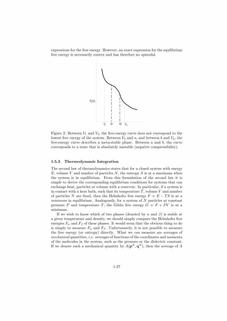
expressions for the free energy. However, an exact expression for the equilibriumfree energy is necessarily convex and has therefore no spinodal.

V1 V2

F(V)

a b

Figure 2: Between V1 and V2, the free-energy curve does not correspond to thelowest free energy of the system. Between V2 and a, and between b and V2, thefree-energy curve describes a meta-stable phase. Between a and b, the curvecorresponds to a state that is absolutely unstable (negative compressibility).

1.5.3 Thermodynamic Integration

The second law of thermodynamics states that for a closed system with energyE, volume V and number of particles N , the entropy S is at a maximum whenthe system is in equilibrium. From this formulation of the second law it issimple to derive the corresponding equilibrium conditions for systems that canexchange heat, particles or volume with a reservoir. In particular, if a system isin contact with a heat bath, such that its temperature T , volume V and numberof particles N are fixed, then the Helmholtz free energy F ≡ E − TS is at aminimum in equilibrium. Analogously, for a system of N particles at constantpressure P and temperature T , the Gibbs free energy G ≡ F + PV is at aminimum.

If we wish to know which of two phases (denoted by α and β) is stable ata given temperature and density, we should simply compare the Helmholtz freeenergies Fα and Fβ of these phases. It would seem that the obvious thing to dois simply to measure Fα and Fβ . Unfortunately, it is not possible to measurethe free energy (or entropy) directly. What we can measure are averages ofmechanical quantities, i.e. averages of functions of the coordinates and momentaof the molecules in the system, such as the pressure or the dielectric constant.If we denote such a mechanical quantity by A(pN ,qN ), then the average of A

1-27

that can be measured in an experiment at constant N , V and T is

〈A〉NV T =

∫

dpNdqNA(pN ,qN ) exp (−βH(pN ,qN ))∫

dpNdqN exp (−βH(pN ,qN ))(1.79)

where H is the Hamiltonian of the system expressed as a function of the mo-menta pN and coordinates qN . kB is Boltzmann’s constant and β = 1/(kBT ).

However, entropy, free energy and related quantities are not simply averagesof functions of the phase-space coordinates of the system. Rather they aredirectly related to the volume in phase space that is accessible to a system.For instance, in classical statistical mechanics, the Helmholtz free energy F isdirectly related to the canonical partition function QNV T :

F = −kBT lnQNV T ≡ −kBT ln

(∫

dpNdqN exp (−βH(pN ,qN ))

hdNN !

)

(1.80)

where h is Planck’s constant and d is the dimensionality of the system.Unlike quantities such as the internal energy, the pressure or polarization,

QNV T itself is a canonical average over phase space. Rather, it is a measurefor the accessible volume of phase space. This is why F or, for that matter, Sor G, cannot be measured directly. We call quantities that depend directly onthe available volume in phase thermal quantities. In experiments, one cannotmeasure the free energy directly. However, derivatives of the free energy withrespect to volume V or temperature T can be measured:

(

∂F

∂V

)

NT

= −P (1.81)

and(

∂F/T

∂1/T

)

V T

= E . (1.82)

As the pressure P and the energy E are mechanical quantities, they can bemeasured. In order to compute the free energy of a system at given temperatureand density, we should find a reversible path in the V − T plane, that links thestate under consideration to a state of known free energy. The change in Falong that path can then simply be evaluated by integration of Eqns. 1.81 and1.82. There are only very few thermodynamic states where the free energy ofa substance is known. One state is the ideal gas phase, another may be theperfectly ordered ground state at T = 0K.

In order to compute the free energy of a dense liquid, one may constructa reversible path to the very dilute gas phase. It is not really necessary togo all the way to the ideal gas. But at least one should reach a state that issufficiently dilute that the free energy can be computed accurately, either fromknowledge of the first few terms in the virial expansion of the compressibilityfactor PV/(NkT ), or that the chemical potential can be computed by othermeans. The obvious reference state for solids is the harmonic lattice. Computing

1-28

the absolute free energy of a harmonic solid is relatively straightforward, at leastfor atomic and simple molecular solids. However, not all solid phases can bereached by a reversible route from a harmonic reference state. For instance,in molecular systems it is quite common to find a strongly anharmonic plasticphase just below the melting line. This plastic phase is not (meta-) stable atlow temperatures.

Artificial paths

Fortunately, in theoretical and numerical studies we do not have to rely on thepresence of a ‘natural’ reversible path between the phase under study and areference state of known free energy. If such a path does not exist, we canconstruct an artificial path. This is in fact a standard trick in statistical me-chanics (see e.g. [11]). It works as follows: Consider a case where we need toknow the free energy F (V, T ) of a system with a potential energy function U1,where U1 is such that no ‘natural’ reversible path exists to a state of known freeenergy. Suppose now that we can find another model system with a potentialenergy function U0 for which the free energy can be computed exactly. Wedefine a generalized potential energy function U(λ), such that U(λ = 0) = U0

and U(λ = 1) = U1. The free energy of a system with this generalized poten-tial is denoted by F (λ). Although F (λ) itself cannot be measured directly in asimulation, we can measure its derivative with respect to λ:

(

∂F

∂λ

)

NV Tλ

=

⟨

∂U(λ)

∂λ

⟩

NV Tλ

(1.83)

If the path from λ = 0 to λ = 1 is reversible, we can use eq. 1.84 to computethe desired F (V, T ). We simply measure 〈∂U/∂λ〉 for a number of values of λbetween 0 and 1.

1.6 Perturbation Theory

The aim of thermodynamic perturbation theory is to arrive at an estimate of thefree energy (and all derived properties) of a many-body system, using as inputinformation about the free energy and structure of a simpler reference system.We assume that the potential energy function of this reference system is denotedby U0 while the potential energy function of the system of interest is denoted byU1. In order to compute the free energy difference between the known referencesystem and the system of interest, we use the linear parametrization of thepotential energy function The free energy of a system with this generalizedpotential is denoted by F (λ). The derivative of F (λ) with respect to λ is

(

∂F

∂λ

)

NV Tλ

=

⟨

∂U(λ)

∂λ

⟩

NV Tλ

(1.84)

and hence we can express the free energy difference F1 − F0 as

F1 − F0 =

∫ 1

0

dλ 〈U1 − U0〉NV Tλ (1.85)

1-29

This expression (first derived by Kirkwood), allows us to put bounds on the freeenergy F1. Consider

(

∂2F

∂λ2

)

NV Tλ

For the linear parametrization considered here, it is straightforward to showthat

(

∂2F

∂λ2

)

NV Tλ

= −β(

⟨

(U1 − U0)2⟩

NV Tλ− 〈(U1 − U0)〉2NV Tλ

)

(1.86)

The important thing to note is that the second derivative of F with respect toλ is always negative (or zero). This implies that

(

∂F

∂λ

)

NV Tλ=0

≥(

∂F

∂λ

)

NV Tλ

and henceF1 ≤ F0 + 〈U1 − U0〉NV Tλ=0 . (1.87)

This variational principle for the free energy is known as the Gibbs-Bogoliubov

F( )l

F0F0F0

F1

l0 1

Figure 3: The perturbation-theory estimate of the free energy of a system isan upper bound to the true free energy. In the figure, the perturbation theoryestimate of F1 is given by the intersection of the dashed line with the line λ = 1.It clearly lies above the true F1. The reason is that the true free energy is alwaysa convex function of λ.

inequality. It implies that we can compute an upper bound to the free energy of

1-30

the system of interest, from knowledge of the average of U1 − U0 evaluated forthe reference system. Note that the present “derivation” was based on classicalstatistical mechanics. However, the same inequality also holds in quantum sta-tistical mechanics [12](a quick-and-dirty derivation is given in appendix A). Ofcourse, the usefulness of Eqn. 1.87 depends crucially on the quality of the choiceof reference system. A good reference system is not necessarily one that is closein free energy to the system of interest, but one for which the fluctuations in depotential energy difference U1−U0 are small. Thermodynamic perturbation the-ory for simple liquids has been very successful, precisely because the structureof the reference system (hard-sphere fluid) and the liquid under consideration(e.g. Lennard-Jones) is very similar. As a result, 〈U1 −U0〉λ hardly depends onλ and, as a consequence, its derivative (Eqn. 1.86) is very small.

1.7 Van der Waals Equation

In some cases, the fluctuation term can be made to vanish altogether. Consider,for instance, the free energy difference between a hard sphere reference systemand a model fluid of particles that have a hard-sphere repulsion and a veryweak, attractive interaction −ǫ that extends over a very large distance Rc. Inparticular, we consider the limit ǫ → 0, Rc → ∞, such that

4π

3R3

cǫ = 2a

where a is a constant. In the limit Rc → ∞, the potential energy of the per-turbed fluid can be computed directly. Within a shell of radius Rc, there willbe, on average, Nc other particles, all of which contribute −ǫ/2 to the potentialenergy of the fluid. For Rc → ∞, the number of neighbors Nc also tends toinfinity and hence the relative fluctuation in Nc becomes negligible (as it is oforder 1/

√Nc). It then follows that the fluctuations in the perturbation (i.e.

U1 − U0) also become negligible and, as a consequence, the Gibbs-Bogoliubovinequality becomes and identity: in this limit of weak, long ranged forces, per-turbation theory becomes exact [9]! I refer to this limit as the “van der Waals”limit, for reason that will become obvious. The free energy per particle of thevan der Waals fluid is

fvdW (ρ, T ) = fHS(ρ, T )− ρa (1.88)

and the pressure is

PvdW = ρ2∂fvdW∂ρ

= PHS(ρ, T )− aρ2 (1.89)

where PHS denotes the pressure of the hard sphere reference system. Of course,van der Waals did not know the equation of state of hard spheres, so he had tomake an approximation [13]:

PHS = ρkBT/(1− ρb) (1.90)

1-31

where b is the second virial coefficient of hard spheres. If we insert Eqn. 1.90in Eqn. 1.89, the well-known van der Waals equation results 4. If, on the otherhand, we use the “exact” equation of state of hard spheres (as deduced fromcomputer simulations), then we can compute the “exact” equation of state of thevan der Waals model (i.e. the equation of state that van der Waals would havegiven an arm an a leg for). Using this approach, Longuet-Higgins and Widom [8]were the first to compute the true phase diagram of the van der Waals model.As an illustration (Figure 4), I have recomputed the Longuet-Higgins-Widomphase diagram, using more complete data about the hard-sphere equation ofstate than were available to Longuet-Higgins and Widom.

0.0 0.5 1.0 1.5ρ

0.0

0.1

0.2

τ

Figure 4: Phase diagram for the van der Waals model. This phase diagram iscomputed by using the hard-sphere system as reference system and adding aweak, long-ranged attractive interaction. Density ρ in units σ−3, where σ is thediameter of the hard spheres. The ‘temperature’ τ is defined in terms of thesecond virial coefficient: B2/B

HS2 ≡ 1− 1/(4τ), where BHS

2 is the second virialcoefficient of the hard-sphere reference system.

1.8 Mean-field theory

The Gibbs-Bogoliubov inequality can be used as a starting point to derive mean-field theory, which can be considered as a systematic approximation for the free

4Van der Waals explained the liquid-vapor transition by assuming that atoms were impen-etrable, spherical objects that exert attractive forces on each other. It should be stressed thatVan der Waals proposed his theory some 40 years before the atomic hypothesis was generallyaccepted. The short-ranged repulsion between atoms was only explained in the 1920’s on basisof the Pauli exclusion principle. And the theory for the attractive (”Van der Waals”) forcesbetween atoms was only formulated by London in 1930.

1-32

energy of a many-body system. For the sake of simplicity, we consider a many-body Hamiltonian of interacting spins (Ising model)

U1 = −J

2

N∑

i=1

∑

jnni

sisj .

The Ising model is not just relevant for magnetic system. In appendix C weshow that a lattice-gas model that can be used to describe the liquid-vaportransition is, in fact, equivalent to the Ising model.

We wish to approximate this model system, using a reference system witha much simpler Hamiltonian, namely one that consists of a sum of one-particlecontributions, e.g.

U0 = −N∑

i=1

hsi

where h denotes the effective “field” that replaces the interaction with the otherparticles. The free energy per particle of the reference system is given by

f0(h) = −kBT ln

∫

ds exp(βhs)

If we only have two spin states (+1 and -1), this becomes

f0(h) = −kT ln(exp(βh) + exp(−βh))

We can easily compute the average value of s in the reference system

〈s〉0 = −∂f0(h)

∂h(1.91)

In the case of spins ±1:〈s〉0 = tanh(βh) (1.92)

Now, we consider the Gibbs-Bogoliubov inequality (Eqn. 1.87

f1 ≤ f0 + 〈u1 − u0〉0= f0 + 〈−J

2

∑

jnni

sisj + hsi〉0

= f0 −J

2z〈s〉20 + h〈s〉0 (1.93)

where, in the last line, we have introduced z, the coordination number of particlei. Moreover, we have used the fact that, in the reference system, different spinsare uncorrelated. We now look for the optimum value of h, i.e. the one thatminimizes our estimate of f1. Carrying out the differentiation with respect to

1-33

h, we find

0 =∂f0 − J

2 z〈s〉20 + h〈s〉0∂h

= −〈s〉0 − (Jz〈s〉0 − h)∂〈s〉0∂h

+ 〈s〉0

= −(Jz〈s〉0 − h)∂〈s〉0∂h

(1.94)

And hence,h = Jz〈s〉0 (1.95)

If we insert this expression for h in Eqn. 1.91, we obtain an implicit equationfor 〈s〉0, that can be solved to yield 〈s〉0 as a function of T . For spins equal to±1,

〈s〉0 = tanh(βJz〈s〉0) (1.96)

The free energy estimate that we obtain when inserting this value of 〈s〉0 inEqn. 1.93 is

fMF = f0 +J

2z〈s〉20 (1.97)

The subscriptMF in this expression stands for the “mean-field” approximation.It is very important to note that the free energy that results from the mean-fieldapproximation is not simply the free energy of the reference system with theeffective field.

1.9 Landau Theory

Matter can occur in many different phases. We can induce transitions from onephase to another, by changing the temperature or pressure of the system, orby varying some other thermodynamic parameter, such as an external electricor magnetic field. At the phase transition, the state of the system changes.But the way in which this change takes place is not the same for all phasetransitions. At a phase transition, the temperatures, pressures and chemicalpotentials of the coexisting phases are the same. This implies that the Gibbsfree energies of coexisting phases are equal. But,as was first pointed out byEhrenfest [14], phase transitions can be classified according to the behavior ofthe derivatives of the Gibbs free energy. If the first derivatives of the Gibbs freeenergy (i.e. V and S) are discontinuous, then the transition is called a ”first-order” phase transition. If the first derivatives are continuous, but the secondare not, then the transition is called a “second-order” phase transition, and soon... In the light of the modern theory of critical phenomena, this classificationcannot strictly be maintained. However, the Ehrenfest classification provides,at the very least, a useful language to discuss the difference between first-orderand continuous phase transitions.

Can we predict whether a give phase transition will be of first order or not?This is the question that Landau addressed in 1937 [15, 16]. Surprisingly, the

1-34

answer is yes (for the purists ”mostly, yes”). And, even more surprisingly, theanswer can be given without much detailed knowledge of the intermolecularinteractions. What is crucial, though, is the symmetry of the system. As Lan-dau already pointed out in his first paper [15], a symmetry is either there or notthere. Unlike the density, the symmetry of a system cannot change continuously.In this respect, Landau says, a so-called continuous phase transformation thatinvolves a symmetry change, is less “continuous” then the first-order transforma-tion from liquid to vapor, that can also be carried out continuously by followinga path around a critical point.

To formulate the Landau theory of phase transitions, we need to quantifythe symmetry properties of the free energy of the system. To be more precise,we must define a quantity that provides a measure for the degree of ordering ofa system. In order to formulate the theory, we need to introduce a new concept:the order parameter. When a phase transition involves a change in symmetry ofthe system (e.g. the transition from an isotropic liquid to a crystalline solid, orthe transition from a para-magnetic to a ferromagnetic phase) then it is usefulto use an order parameter that is zero in the disordered phase, and becomes non-zero in the ordered phase. In the case of magnetic systems, the magnetization issuch an order parameter. In section 1.4.1, we showed that it is possible to relatea free energy to the probability to observe a particular spontaneous fluctuationin the value of an observable quantity (see Eqn. 1.78. For an observable M , wehave:

F (N, V, T,M = x) = −kBT lnP(M = x) + constant (1.98)

where P(M = x) denotes the probability that, due to a spontaneous fluctuation,the observable M equals x. Clearly, the most likely situation corresponds to themaximum of P , and hence to the minimum of F .

We now consider the situation that M is the order parameter that distin-guishes the ordered phase (usually at low temperatures) from the disorderedphase (usually at high temperatures). In the disordered phase, the most likelyvalue of M is zero. In the ordered phase, the minimum of F corresponds to anon-zero value of M . We now make the assumption that we can expand thefree energy of the disordered phase in powers of the order-parameter M .

F (N, V, T,M) = F (N, V, T, 0) + aM + bM2 + cM3 + dM4 + · · · (1.99)

As this is an expansion of the free energy of the disordered phase, every termmust be invariant under all symmetry operations of the disordered phase. Thisimplies that the term linear in M must vanish (because if M itself had thefull symmetry of the disordered phase, it would not be a good measure for thechange in symmetry at the phase transition). In general the quadratic term inEqn. 1.99 will be non-zero. The cubic term may or may not vanish, dependingon nature of the order parameter. To give an example: if we consider sponta-neous magnetization, then the fluctuations with magnetization +M and −Mare equally likely, and hence the Landau free energy (Eqn. 1.99) must be aneven function of M . But in other cases (e.g. the fluid-solid transition or theisotropic-nematic transition), the cubic term in the expansion is not symmetry

1-35

forbidden. This is easy to see in the case of the isotropic-nematic transition.In the isotropic phase, the distribution of molecular orientations has sphericalsymmetry. In the nematic phase, the distribution has cylindrical symmetry. Apositive nematic order parameter corresponds to the case that the moleculestend to align parallel to the symmetry axis: the distribution function of molec-ular orientations resembles a prolate ellipsoid. If the nematic order parameteris negative, then the molecules have a propensity to align perpendicular to thesymmetry axis. In that case, the orientational distribution function is more likean oblate ellipsoid. These two distributions are physically distinct, and hencethere is no symmetry between states with positive and negative order parameter.

We assume that the coefficients b, c, d etc. in Eqn. 1.99 all are continuousfunctions of temperature. For the study of phase transitions, we focus on thetemperature regime where b changes sign at a temperature Tc. Close to Tc wecan ignore the temperature dependence of the other coefficients. Then we canwrite

F (N, V, T,M) ≈ F (N, V, T, 0) + α(T − Tc)M2 + cM3 + dM4 + · · · (1.100)

Now we can distinguish several situations. First, we consider the case that theLandau free energy is an even function ofM and that the coefficient d is positive:

F (N, V, T,M) ≈ F (N, V, T, 0) + α(T − Tc)M2 + dM4 (1.101)

Above Tc, the most minimum of the free energy corresponds to the state M = 0.In other words, above Tc, the disordered phase is stable. Below Tc, the pointM = 0 changes form a minimum in the free energy to a local maximum. Theminimum of the free energy is easily found to be

M = ±√

α(Tc − T )

2d

The free energy below Tc is

F (N, V, T,M) ≈ F (N, V, T, 0)− α2(T − Tc)2

4d(1.102)

Note that, in this case, ordering sets in at Tc and that the free energy and itsfirst derivative are continuous at the transition. However, the heat capacityexhibits a jump at the phase transition. This is characteristic for a second-order phase transition in the Ehrenfest classification. An interesting alternativesituation is that the coefficient d is negative. Then we have to consider the nextnon-vanishing term in the series. Let us assume that the coefficient f of M6

is positive. Then it is easy to show that at high temperatures, the absoluteminimum of the free energy corresponds to the point M = 0. However, when

T − Tc =d2

4fα

The point M = 0 is still a local minimum, but no longer the global minimum.The global minimum of the free energy jumps to the point M = ±

√

|d/2|. Of

1-36

course, the free energy itself is continuous at the transition. But now thereis a discontinuity in its first derivative: in the Ehrenfest language, we have afirst-order phase-transition.

Finally, let us consider the very important case that F contains odd powersof M :

F (N, V, T,M) ≈ F (N, V, T, 0) + α(T − Tc)M2 + cM3 + dM4 + · · · (1.103)

We assume that d is positive. At high temperatures, the global minimum of thefree energy is a M = 0. But at the point

T − Tc =c2

4dα

the minimum jumps to M = −c/2 and a first-order phase transition takesplace. Hence, according to Landau theory, both the freezing transition and theisotropic-nematic transition must be first order.

The Landau theory is a very useful way to analyze phase transitions. But itis not rigorous. In particular, it makes the assumption that the state of a systemis determined by the minimum of Landau free energy. Fluctuations around thatminimum are ignored. In practice, fluctuations may have a large effect on thebehavior of a system near a phase transition.

A Quantum Gibbs-Bogoliubov inequality

We start with the expansion of the exponential operator to second order in theperturbation5:

e−β(H0+λH1) = e−β(H0+λH1)o− λβ

∫ 1

0

ds e−β(1−s)H0H1e−βsH0 (A.1)

+λ2β2

∫ 1

0

ds

∫ s

0

du e−β(1−s)H0H1e−β(s−u)H0H1e

−βuH0 +O(λ3)

and take the trace and divide by Q(0) = Tr e−β(H0+λH1)o:

Q(λ)

Q(0)= 1− λβ 〈H1〉H0

+ λ2β2

∫ 1

0

ds

∫ s

0

duTr e−β(1−s+u)H0H1e

−β(s−u)H0H1

Tr e−β(H0+λH1)o(A.2)

where we have used (and will use repeatedly below) the fact that TrAB =TrBA, even if A and B do not commute, and that for any operator: exp(λA) exp(µA) =exp(λ+ µ)A. Take the opposite of the logarithm, and keep terms up to secondorder in λ:

βF (λ)−βF (0) = λβ 〈H1〉H0+λ2β2

[

1

2〈H1〉2H0

−∫ 1

0

ds

∫ s

0

dαTr e−β(1−α)H0H1e

−βαH0H1

Tr e−β(H0+λH1)o

]

(A.3)

5Obtained from recursive use of the equality: e(A+B)t = eAt +∫t

0ds eA(t−s)Be(A+B)s for

t = 1, A = −βH0, and B = −βλH1. The derivation of this result is straightforward whenconsidering eAt d

dte−Ate(A+B)t.

1-37

where we have also made the change of variable α = s− u.

To prove Gibbs-Bogoliubov inequality, we only need to show that F is con-cave at λ = 0 (by shifting the origin, we can then conclude that it is con-cave everywhere), i.e. that the term between brackets is negative. To showthis, we note that for a hermitian operator H such as the Hamiltonian, andfor any real scalar λ, (expλH)† = expλH . The idea is then to consider thescalar product (A,B) 7→ TrA†B for which the Cauchy-Schwartz inequality is:|TrA†B|2 ≤ (TrA†A)(TrB†B). We can now rewrite:

Tr e−β(1−α)H0H1e−βαH0H1 = Tr e−β 1−α

2H0H1e

−β α2H0e−β α

2H0H1e

−β 1−α2

H0 = TrA†A(A.4)

with A = exp(−β α2H0)H1 exp(−β 1−α

2 H0). The trick is to apply the Cauchy-

Schwartz inequality by introducing B = exp(−β2H0):

Tr e−β(1−α)H0H1e−βαH0H1 ≥

[

Tr e−β 1−α2

H0H1e−β α

2H0e−

β

2H0

]2

Tr e−β

2H0e−

β

2H0

=

[

Tr e−βH0H1

]2

Tr e−βH0

= 〈H1〉2H0Tr e−βH0

(A.5)Thus a lower bound for the double integral in (A.3) is:

∫ 1

0

ds

∫ s

0

dαTr e−β(1−α)H0H1e

−βαH0H1

Tr e−β(H0+λH1)o≥ 〈H1〉2H0

∫ 1

0

ds

∫ s

0

dα =1

2〈H1〉2H0

(A.6)which proves that F ′′(λ = 0) ≤ 0, and hence the Gibbs-Bogoliubov inequality.

This elegant derivation is due to Dr Benjamin Rotenberg.

B Virial pressure

Clausius proposed the following, very general, method to derive an expressionfor the pressure of a many body system. Consider a system of N -particles in avolume V at total energy E. As the volume and the total energy of the systemare finite, the following quantity

V ≡N∑

i=1

ri.pi

must be bounded. This means that, for a system in equilibrium, the averagevalue of V must vanish

V = 0

where the bar over V denotes the time average. It the follows that

N∑

i=1

ri.pi +N∑

i=1

ri.pi = 0

2-38

Usingri = pi/mi

andpi = fi ,

where fi is the force on particle i, we can write

N∑

i=1

p2i /mi +N∑

i=1

ri.fi = 0

The first term on the left is simply twice the kinetic energy of the system. Usingthe equipartition theorem, we can write this as 3NkBT . We then get

3NkBT +N∑

i=1

ri.fi = 0

Next, we write fi as the sum of the force due to intermolecular interactions,and the force due to interactions with the wall of the container. Let us considerthe contribution to virial due to the interaction with a surface element dS ofthe wall of the container. We denote the position of this surface element by rS .Whenever a particle collides with this surface element, its coordinate is given byrS . Hence, collisions with this surface element make the following contributionto the force virial

(

N∑

i=1

ri.fi

)(dS)

=

N∑

i=1

rS .f(dS)i

= rS .

N∑

i=1

f(dS)i

= rS .F(dS)tot

= rS .(−P )dS , (B.1)

where the superscript (dS) indicates that we only consider forces due to theelement dS of the container wall. In the last line of the above equation, we haveused the fact that the average of the total force exerted on an area dS equalsPdS and hence the force exerted by that area on the particles is −PdS. Wecan now integrate over the entire surface of the container to obtain

(

N∑

i=1

ri.fi

)

wall

= −P

∮

S

rS .dS (B.2)

Using Gauss’s theorem, this can be rewritten as

−P

∮

S

rS .dS = −P (∇.r)V

2-39

In 3D, ∇.r = 3, and hence

−P

∮

S

r.dS = −3PV

With this result, we can write

3NkBT +N∑

i=1

ri.f interi − 3PV = 0

or

PV = NkBT +1

3

N∑

i=1

ri.f interi

which should be compared to the result that we obtained in Eqn. 1.54

P =NkBT

V+

⟨

N∑

i=1

1

3Vri.fi

⟩

(B.3)

C Ising model and Lattice gas

The Ising model for a lattice of interacting magnetic spins is among the mostwidely used models in physics because many other models can be mapped ontoit. As an example, we consider the relation between the Ising model and alattice gas. The lattice gas model is a simple model to describe the liquid-vapor transition. Let us first consider the Ising model. In the Ising model,neighboring parallel spins have an interaction energy −J , anti-parallel spinshave an interaction energy +J . We denote the value of the spin on lattice sitei by si. si can take on the values +1 and -1. The “Ising Hamiltonian” is givenby

HI = −J

2

N∑

i=1

∑

jnni

sisj .

In the presence of a magnetic field B, the Hamiltonian becomes

HI = −J

2

N∑

i=1

∑

jnni

sisj −BN∑

i=1

si .

The partition function of the Ising model can be written as:

QI =∑

s

exp(−β(−J

2

N∑

i=1

∑

jnni

sisj −B

N∑

i=1

si))

where β = 1/kT and s denotes all possible sets of spin values, i.e (s1 = 0, 1),(s2 = 0, 1) · · · (sN = 0, 1).

3-40

Now consider a gas on a lattice with M sites. There can be at most oneparticle per lattice site. Neighboring particles have an interaction energy −ǫ.The Hamiltonian is

HLG = − ǫ

2

N∑

i=1

∑

jnni

ninj .

where ni denotes the number of particles (0 or 1) on site i. The partitionfunction is

QLG(M) =∑

n′

exp(−β(− ǫ

2

N∑

i=1

∑

jnni

ninj))

where n′ denotes the set of occupation numbers that satisfy∑

i ni = M .It turns out to be more convenient to consider the Grand-canonical partitionfunction Ξ.

Ξ =

N∑

M=0

∑

n

exp(−β(− ǫ

2

N∑

i=1

∑

jnni

ninj))eβµM

Now we can change the order of the summation to convert the sum in an unre-stricted sum over n1, n2, · · · , nN :

Ξ =∑

n

= exp(−β(− ǫ

2

N∑

i=1

∑

jnni

ninj)− µ∑

ni)

It is immediately obvious that the grand-canonical partition function of thislattice gas is identical in form to the canonical partition function of an Isingmodel in a magnetic field, with the identification s = 2n− 1, J = ǫ and B = µ.

3-41

References

[1] D. Chandler, Introduction to Modern Statistical Mechanics (Oxford Uni-versity Press, New York, 1987).

[2] J.-L. Barrat and J.-P. Hansen, Basic Concepts for Simple and ComplexLiquids (Cambridge U.P., Cambridge, 2003).

[3] P.M. Chaikin and T.C.Lubensky, Principles of Condensed Matter Physics(Cambridge U.P., Cambridge, 2000).

[4] J. L. Lebowitz, J. K. Percus, and L. Verlet, Phys. Rev. 153, 250 (1967).

[5] J. I. Siepmann, I. R. McDonald, and D. Frenkel, Journal of Physics Con-densed Matter 4, 679 (1992).

[6] W. W. Wood, J. Chem. Phys. 48, 415 (1968).

[7] V. F. Weisskopf, Trans NY Acad. Sci. Ser. II 38, 202 (1977).

[8] H.C. Longuet-Higgins and B. Widom, Mol. Phys. 8, 549 (1964).

[9] P.C. Hemmer and J.L. Lebowitz, in Critical Phenomena and Phase Tran-sitions 5b, edited by C. Domb and M. Green (Academic Press, New York,1976).

[10] P. Bolhuis and D. Frenkel, Phys. Rev. Lett. 72, 2211 (1994).

[11] J. P. Hansen and I. R. McDonald, Theory of Simple Liquids (AcademicPress, (2nd edition), London, 1986).

[12] R. P. Feynman, Statistical Mechanics (Benjamin, Reading (Mass.), 1972).

[13] J.S.Rowlinson, in Studies in Statistical Mechanics, Vol. XIV, edited byJ.L.Lebowitz (North Holland, Amsterdam, 1988).

[14] P. Ehrenfest, Proc. Amsterdam Acad. 36, 153 (1933).

[15] L.D. Landau, Z. Phys. Sovjetunion 11, 26 (1937).

[16] L.D. Landau, Z. Phys. Sovjetunion 11, 545 (1937).

3-42