lecture_p

7/28/2019 lecture_p

http://slidepdf.com/reader/full/lecturep 1/113

Mathematical Foundations of Electromagnetic Field Theory (MFEFT)

Dr.-Ing. Rene Marklein

[email protected]

FG Electromagnetic TheoryFB 16 Electrical Engineering / Computer Science

University of Kassel

WS 2007/2008

Dr.-Ing. Rene Marklein (University of Kassel) Mathematical Foundations of EFT (MFEFT) WS 2007/2008 1 / 113

7/28/2019 lecture_p


FB16-2508 Mathematical Foundations of Electromagnetic Field Theory(MFEFT) - Lectures / Exercises

Lectures

Dr.-Ing. Rene Marklein

Tu 14.00-15.30, Room 2104/WA71, Start: 23.10.2007

Exercises

Prashanth Kumar Chinta, M.Sc.Th 11.30-13.00, every 2nd week, Room 2104/WA71, Start: 01.11.2007


7/28/2019 lecture_p


MFEFT - Outline

1 Introduction

2 Vector and Tensor Algebra

3 Vector and Tensor Analysis

4 Distributions

5 Complex Analysis

6 Special Functions

7 Fourier Transform

8 Laplace Transform


7/28/2019 lecture_p


Lecture 1: Introduction; Vector- and Tensor Algebra; Position Vector andCoordinate Systems


I d i

7/28/2019 lecture_p


Introduction

MFEFT - Lecture 1

1 Introduction


Position Vector and Coordinate SystemsCartesian CoordinatesEinstein’s Summation ConventionDifferentiation of the Position Vector; Kronecker Symbol (Kronecker Delta)Cylinder Coordinate SystemOrthogonal Curvilinear Coordinate SystemSpherical Coordinate SystemDupin Coordinates

Vectors: Scalar Product; Vector Product; Dyadic ProductScalar ProductVector ProductDyadic ProductComplex Vectors

TensorsDefinition


4 Distributions

5 Complex Analysis

6 Special Functions

7 Fourier Transform

8 Laplace Transform


Int od ction

7/28/2019 lecture_p


Introduction

Introduction

In the following lecture series we are going to discuss the mathematical basis of electromagnetic fields and waves as solutions of the theory of James Clerk Maxwell.

We do not claim completeness!

We provide the essential results and facts without detailed proofs.

We try to provide a sketch of the derivations and explain, illustrate, and discuss themathematical relations.

We follow in principle the first book chapter of the German manuscript by Karl-J¨ org

Langenberg [2002]:

[Langenberg , 2002] K.-J. Langenberg: Theory of Electromagnetic Waves. Manuskript,Universitat Kassel, Kassel, 2002 (in German).

→ You can get a copy of the CD with this Manuscript!Contact: Dr.-Ing. Rene Marklein in his office or wire e-mail: [email protected]


Introduction

7/28/2019 lecture_p


Introduction

Introduction

Our idol is the mathematician Gustav Doetsch, who wrote books for engineers about theFourier and Laplace transform as well as the theory of distributions. We point out the bookchapter [Doetsch, 1967]:

[Doetsch, 1967] G. Doetsch: Funktionaltransformationen . In: R. Sauer, I. Szabo (Eds.):Mathematische Hilfsmittel des Ingenieurs, Teil I . Springer-Verlag, Berlin, 1967.

We are going to follow the books:Vector and Tensor Algebra by Hollis Chen [1983]:

[Chen, 1983] H.C. Chen: Theory of Electromagnetic Waves . McGraw-Hill, New York,1983.

Functional Theory by Heinrich Behnke and Friedrich Sommer [Behnke & Sommer , 1965]:

[Behnke & Sommer , 1965] H. Behnke, F. Sommer: Theorie der analytischen

Funktionen einer komplexen Veranderlichen. Springer-Verlag, Berlin 1965.Vector and Tensor Analysis by the 4th Volume of the Mathematics for Engineers by K. Burg,

H. Haf und F. Wille (”‘BHW”’) Burg et al.[1990]:

[Burg et al., 1990] K. Burg, H. Haf, F. Wille: Hohere Mathematik f¨ ur Ingenieure, Band

IV: Vektoranalysis und Funktionentheorie . B.G. Teubner, Stuttgart 1990.The main features about Special Functions are derived from the Book Theory of Ordinary

Differential Equations in the Complex Domain by Smirnow [1959]:

[Smirnow , 1959] W.I. Smirnow: Lehrgang der h¨ oheren Mathematik, Teil III,2 . VEBDeutscher Verlag der Wissenschaften, Berlin 1959.Dr.-Ing. Rene Marklein (University of Kassel) Mathematical Foundations of EFT (MFEFT) WS 2007/2008 7 / 113

Vector and Tensor Algebra

7/28/2019 lecture_p



MFEFT - Lecture 1

1 Introduction




TensorsDefinition


4 Distributions

5 Complex Analysis

6 Special Functions

7 Fourier Transform

8 Laplace Transform



7/28/2019 lecture_p



Electromagnetic Fields

Electromagnetic Fields; Vector Fields; Maxwell’s Equations

Electromagnetic Fields are Vector Fields, which are a function of Time t and thethree-dimensional Position Vector R; Maxwell’s Equations

∇

×E(R, t) =

−∂ B(R, t)

∂t −Jm

(R, t)

∇×H(R, t) =∂ D(R, t)

∂t+ Je(R, t)

∇·D(R, t) = e(R, t)

∇·B(R, t) = m(R, t)

describing the Physics of their interaction through the change in Time and Space, this requiresMathematical Tools to describe such changes of Vector Fields and their Algebraic Interrelation.



7/28/2019 lecture_p


g

Literature

Further literature of the topic vector/tensor algebra and analysis

[Tai , 1992] C. T. Tai: Generalized Vector and Dyadic Analysis. IEEE Press, New York 1992

[Bourne & Kendall , 1988] D. E. Bourne, P. C. Kendall: Vektoranalysis . TeubnerStudienbucher, B. G. Teubner, Stuttgart 1988

[Teichmann, 1963] H. Teichmann: Physikalische Anwendungen der Vektor- und

Tensorrechnung . Bibliographisches Institut, Mannheim 1963

[Fetzer , 1978] V. Fetzer: Mathematik f¨ ur Elektrotechniker, Band 1. Huthig Verlag,Heidelberg 1978

[Spiegel , 1977] M. S. Spiegel: Vektoranalysis . Schaum’s Outline, McGraw-Hill, Hamburg,

1977.[Morse & Feshbach, 1953] P. M. Morse, H. Feshbach: Methods of Theoretical Physics, Part

I and Part II. McGraw-Hill, New York, 1953.


Vector and Tensor Algebra Position Vector and Coordinate Systems

7/28/2019 lecture_p


g y

MFEFT - Lecture 1

1 Introduction




TensorsDefinition


4 Distributions

5 Complex Analysis

6 Special Functions

7 Fourier Transform

8 Laplace Transform



7/28/2019 lecture_p


Cartesian Coordinate SystemCartesian Coordinates; Unit Vectors, Magnitude of the Position Vector

x , y, z Coordinate Axes as per Heinrich Hertz[Hertz , 1890] (see Fig. ):

”‘Wir nehmen an, dass das benutzte

Coordinatensystem der x , y, z von solcher

Beschaffenheit ist, dass, wenn die Richtung der

positiven x von uns aus nach vorn, die der positiven

z von uns aus nach oben geht, alsdann die y von

links nach rechts hin wachsen.”’

English translation: ”‘We assume that the used

coordinate system of x , y, z is in such a way, that, if

the direction of the positive x points from us to the

front, the positive z points from us upwards, and yincreases from left to right”’.

[Hertz , 1890] H. R. Hertz: Uber dieGrundgleichungen der Elektrodynamik furruhende Korper. Nachrichten von der

K¨ oniglichen Gesellschaft der Wissenschaften

und der Georg-August-Universitat zu

G¨ ottingen, pp. 106-149; nachgedruckt in

Annalen der Physik , Vol. 40, pp. 577-624,1890.

..

..

..

..

..

..

..

..

..

..

..

..

..

..

..

..

..

..

..

..

..

..

..

..

..

..

..

..

..

..

..

..

..

..

..

..

..

..

..

..

..

..

..

..

..

..

..

..

..

..

..

..

..

..

..

..

.............................

..

..

..

..

..

..

..

..

..

..

..

..

..

..

..................

................

...............................................................................................................................................................

................

...........................

..............................................................................................................

................

O

x

y

z

Figure 1: Cartesian Coordinates of thespatial point P and the related position

vector



7/28/2019 lecture_p


Cartesian Coordinate SystemCartesian Coordinates; Unit Vectors, Magnitude of the Position Vector

Cartesian Coordinates; Unit Vectors,Magnitude of the Position Vector

Cartesisan Coordinates: x , y, z

or x1, x2, x3 (or xi with i = 1, 2, 3))

in the limits −∞ < x < ∞,

−∞ < y < ∞, −∞ < z < ∞Orthonormal Unit Vectors: ex, ey, ez

with |ex| = |ey| = |ez | = 1a

and ex ⊥ ey ⊥ ezb

The straight line from the coordinate

origin O to the (observation) point P isillustrating the position vector R of P ,

the magnitude of the position vector is|R| = R =

x2 + y2 + z2

a| · | stands for the magnitude of the argumentb ⊥ stands for perpendicular

.........

.........

.........

...........................

.........

.........

.........

.........

.........

.........

.........

.........

.........

.........

.........

.........

.........

.........

.........

........................

..

...............

.

...............

.................................................................................................................................................................................................. .......................................................................................................................................................................................................

...........................................................................................................................................................................

..........................

..........................

.........................................................................................................................................

......................................................................................................................................................................................................

.........

.........

.........

.........

.........

.........

.........

.........

.........

.........

.........................

.........

.........

.........

.........

.........

.............

..........................

..........................

..........................

.....................

u

..

..

..

..

..

..

..

..

..

..

..

..

..

.................................

..

..

..

..

..

..

..

..

..

..

..

..

..

..

..

..

..

..

..

..

..

..

..

..

..

..

..

..

..

..

..

..

..

..

..................

................

..

..

..

..

..

..

..

..

..

..

..

...........................

..

..

..

..

..

...............

...

.............

...

.............................................................................

................

...................................................................

................

O

x

y

z

z

x

y

P (x,y,z)

Rez

ex

ey

Figure 2: Cartesian Coordinates of the spatialpoint P and the related position vector



7/28/2019 lecture_p


Scalar and Vectorial (Vector)Components

Scalar (Vector)ComponentsThe projections of the vector onto the orthonormal unit vectors ex, ey, ez yield the Scalar(Vector)Components Rx, Ry, Rz of R:

Rx = ex ·R (1)

Ry = ey ·R (2)

Rz = ez ·R (3)

Vectorial (Vector)Components

If we multiply the scalar (vector)components with the relating unit vectors, we obtain theVectorial (Vector)Components Rx, Ry, Rz of R:

Rx = Rx ex = (ex ·R) ex (4)

Ry = Ry ey = (ey ·R) ey (5)

Rz = Rz ez = (ez ·R) ez (6)



7/28/2019 lecture_p


Cartesian Coordinate SystemComponent Representation of the Position Vector in the Cartesian Coordinate System

Component Representation of the PositionVector in the Cartesian Coordinate System

According to the rules of vector addition itfollows that the component representationof the Position Vector R in the CartesianCoordinate System is

R = Rx ex + Ry ey + Rz ez (7)

= x ex + y ey + z ez (8)

Cartesian Coordinates of the spatial pointP and the related position vector

.........

.........

.........

.........

.........

.........

.........

.........

.........

.........

.........

.........

.........

......................

.........

.........

.........

.........

.........

.........

.........

.........

...................

................

.................................................................................................................................................................................................. .................................................................................................................................................................................

......................

...........................................................................................................................................................................

.............................................

..........................

......................................................................................................................

..........................................................

............................................................

........................................................................................................................................................................................................................................................................

..............................................

..........................

................

u

..

..

..

..

..

..

..

..

..

..

..

..

..

..

..

..

..

..

..

..

..

..

..

..

..

..

..

..

..

..

..

..

..

..

..

..

..

..

..

..

..

..

..

..

..

..

..

..

..

..

..

..

..

..

..

..

..

..

..

..

..

..

..

..

.................

................

..

..

..

..

..

..

..

..

..

..

..

..

..

..

..

..

..

..

..

..

..

..

..

..

..

..

..

..

..

..

.................

................

.............................................................................

................

...................................

.............................

..

.

................

O

x

y

z

z

x

y

P (x,y,z)

Rez

ex

ey



7/28/2019 lecture_p


Cartesian Coordinate SystemComponent Representation of the Position Vector in the Cartesian Coordinate System

Component Representation of the PositionVector in the Cartesian Coordinate System

Using the coordinates x1, x2, x3 it followsfor the Position Vector R in the CartesianCoordinate System

R = xex + y ey + z ez (9)= x1 ex1 + x2 ex2 + x3 ex3 (10)

The advantage of this notation is that wecan write the position vector in form of asum:

R = x1 ex1 + x2 ex2 + x3 ex3 (11)

=3

i=1

xi exi (12)

Cartesian Coordinates of the spatial Point P and the related Position Vector R

.........

.........

.........

.........

.........

.........

.........

.........

.........

.........

.........

.........

.........

.........

...................

.........

.........

.........

.........

.........

.........

.........

......................

................

.................................................................................................................................................................................................. .................................................................................................................................................................................

......................

...........................................................................................................................................................................

.....................................................

........................................................................................................................................

..................................................................

............................................

.......................................................................................................................................................................................................................................................................................

...............................................

..........................

........

u

..

..

..

..

..

..

..

..

..

..

..

..

..

..

..

..

..

..

..

..

..

..

..

..

..

..

..

..

..

..

..

..

..

..

..

..

..

..

..

..

..

..

..

..

..

..

..

..

..

..

..

..

..

..

..

..

..

..

..

..

..

..

..

..

.................

................

..

..

..

..

..

..

..

..

..

..

..

..

..

..

..

..

..

..

..

..

..

..

..

..

..

..

..

..

..

..

.................

................

.............................................................................

................

...........................

........................................................

O

x = x1

y = x2

z = x3

x = x1

y = x2

z = x3

P (x,y,z)

= P (x1, x2, x3)R

ez = ex3

ex= e

x1

ey = ex2



7/28/2019 lecture_p


Einstein’s Summation Convention

Einstein’s Summation Convention

The numbered form of Eq. (10) allows a short hand notation using Einstein’s summationconvention:

R =

3i=1

xi exi (13)

def = xi exi , (14)

i. e., one can delete the sum sign and say:If an index appears only on one side of an equation and more than two times, we have to build a

sum from 1 to 3.



7/28/2019 lecture_p


Differentiation of the Position Vector

Differentiation of the Position Vector

Differentiation of the xith cartesian coordinate of the position vector with regard to the xjthcoordinate is

∂

∂xj

R =∂

∂xj

xi exi

(15)

= exi∂xi

∂xj+ xi

∂ exi∂xj = 0

(16)

= exi∂xi

∂xj

. (17)

It follows for the term ∂xi/∂xj :

∂xi

∂xj

=

0 for i = j

1 for i = j .(18)



7/28/2019 lecture_p


Cartesian Coordinate SystemDifferentiation of the Position Vector; Kronecker Symbol (Kronecker Delta)

Differentiation of the Position Vector; Kronecker Symbol (Kronecker Delta)

The right-hand side (RSH) of the last Eq. (18) is representing the properties of the KroneckerSymbol (Kronecker Delta):

δij =

0 for i = j

1 for i = j(19)

It follows for the above mentioned differentiation of the position vector with regard to the xjthcoordinate

∂

∂xj

R =∂

∂xj

(xiexi) (20)

= exi∂xi

∂xj = δij

(21)

= exi δij . (22)



7/28/2019 lecture_p


Cartesian Coordinate SystemDifferentiation of the Position Vector; Kronecker Symbol

Differentiation of the Position Vector in Cartesian Coordinates; Kronecker Symbol

The term exi δij can be simplified to

exi δijj=i= exi (23)

or (24)

i=j= exj , (25)

i. e., one can either replace i by j or j by i, because δij is only for i = j unequal of null. We findfor i = j:

∂

∂xj

R = exi δij (26)

i=j= exj δij (27)

= exj . (28)



7/28/2019 lecture_p


Cartesian Coordinate SystemDifferentiation of the Position Vector; Kronecker Symbol

Keep in Mind!

Obviously, we obtain the three orthogonal unit vector exj , j = 1, 2, 3 by differentiating theposition vector with regard to the cartesian coordinate xj :

∂

∂xj

R = exj . (29)

Example (Differentiation of the Position Vector; Kronecker Symbol)

If xjj=1= x1 = x it follows:

With the application of the summation con-vention:

∂

∂x1R =

∂

∂x1(xi exi) (30)

= exi∂xi

∂x1 = δi1

(31)

= exi δi1 (32)

= ex1 . (33)

Without the summation convention:

∂

∂xR =

∂

∂x x ex + y ey + z ez (34)

=∂

∂xx

= 1

ex +∂

∂xy

= 0

ey +∂

∂xz

= 0

ez

(35)

= ex . (36)



7/28/2019 lecture_p


Lecture 2: Position Vector and Coordinate Systems (cont.)



7/28/2019 lecture_p


MFEFT - Lecture 2

1 Introduction




TensorsDefinition


4 Distributions5 Complex Analysis

6 Special Functions

7 Fourier Transform

8 Laplace Transform



7/28/2019 lecture_p


Cartesian Coordinate SystemPosition Unit Vector

Position Unit Vector

The Unit Vector of the Position Vector R is R (Unit Position Vector):

R =R

R(37)

=xex + yey + zez

x2 + y2 + z2. (38)

If we build ∂R/∂xi exi for i = 1, 2, 3, it follows with the summation convention the form

∂R

∂xi

exi = ∇R (39)

= R (40)

with the so-called Del Operatora ∇

∇ =∂

∂xex +

∂

∂yey +

∂

∂zez =

3i=1

∂

∂xi

exi =∂

∂xiexi . (41)

aDel Operator = Nabla Operator



C i C di S

7/28/2019 lecture_p


Cartesian Coordinate SystemExample: Proof of ∇R = R

Example (Proof of ∇R = R)

∂R

∂xiexi =

3i=1

∂R

∂xi

exi (42)

=∂R

∂x1ex1 +

∂R

∂x2ex2 +

∂R

∂x3ex3 (43)

= ∂ ∂x1

x21 + x22 + x23 ex1 + ∂

∂x2

x21 + x22 + x23 ex2 + ∂

∂x3

x21 + x22 + x23 ex3 .

(44)

We find by applying the chain rule

∂

∂x1 x21 + x2

2 + x2

3 =

∂

∂x1 x

2

1 + x

2

2 + x

2

3 12 =

1

2 x

2

1 + x

2

2 + x

2

3− 12

Derivative of outer function

2 x1 Derivative of inner function

(45)

=x1

x21 + x22 + x2312

=x1

x21 + x22 + x23

. (46)



C i C di S

7/28/2019 lecture_p




Analog follows for the other two deriviatives

∂

∂x2 x21 + x22 + x23 =

x2

x21 + x2

2 + x2

3

(47)

∂

∂x3

x21 + x22 + x23 =

x3 x21 + x22 + x23

(48)

or in general

∂ ∂xi

x21 + x22 + x23 = xi x21 + x22 + x23

i = 1, 2, 3 . (49)



C t i C di t S t

7/28/2019 lecture_p




We summarize:

∂R

∂xi

exi

=∂

∂x1 x21 + x22 + x23 ex1 +

∂

∂x2 x21 + x22 + x23 ex2 +

∂

∂x3 x21 + x22 + x23 ex3 (50)

= x1 x21 + x22 + x23

ex1 + x2 x21 + x22 + x23

ex2 + x3 x21 + x22 + x23

ex3 (51)

=1

x21 + x22 + x23

x1ex1 + x2ex2 + x3ex3

(52)

=x1e

x1

+ x2ex2

+ x3ex3

x21 + x22 + x23(53)

=R

R(54)

= R . (55)



C t i C di t S t

7/28/2019 lecture_p


Cartesian Coordinate SystemProjection of the Position Vector in the Direction of the Axes of the Cartesian Coordinate System

Projection of the Position Vector in the Direction of the Axes of the Cartesian Coordinate System

If we project the position vector in the direction of the Axes of the Cartesian Coordinates System wefind the components of R:

x = R ·ex (56)

y = R ·ey (57)

z = R ·ez , (58)

this means also

R = (R ·ex)ex + (R ·ey)ey + (R ·ez)ez (59)

Cartesian Coordinates of the spatialpoint P and the related positionvector

.........

.........

.........

.........

.........

.........

.........

.........

.........

.........

.........

.........

.........

.........

.........

...................

.........

.........

.........

.........

.........

.........

......................

................

.................................................................................................................................................................................................. ..................................................................................................................................................................................

.....................

...........................................................................................................................................................................

.......................................

......................................................................................................................................................

...............................................................................

..................

....................................................................................................................................................................................................................................................................................................

...............................................

..........................

........

..

..

..

..

..

..

..

..

..

..

..

..

..

..

..

..

..

..

..

..

..

..

..

..

..

..

..

..

..

..

..

..

..

..

..

..

..

..

..

..

..

..

..

..

..

..

..

..

..

..

..

..

..

..

..

..

..

..

..

..

..

..

..

..

.................

................

..

..

..

..

..

..

..

..

..

..

..

..

..

..

..

..

..

..

..

..

..

..

..

..

..

..

..

..

..

..

.................

................

.............................................................................

................

...............

....................................................................

O

x

y

z

z

x

y

P (x,y,z)

R

ez

ex

ey



(Circular)Cylinder Coordinate System

7/28/2019 lecture_p


(Circular)Cylinder Coordinate SystemCoordinates; Unit Vectors, Magnitude of the Position Vector

Coordinates; Unit Vectors, Magnitude of the Position Vector

Cylinder Coordinates: r,ϕ,z

in the limits 0 ≤ r < ∞, 0 ≤ ϕ < 2π,−∞ < z < ∞; azimuth angle ϕ.

Orthonormal Unit Vectors:er(ϕ), eϕ(ϕ), ez

with |er| = |eϕ| = |ez| = 1

and er ⊥ eϕ ⊥ ezThe straight line from the coordinate

origin O to the (observation) point P is illustrating the position vector R of P , the magnitude of the positionvector is |R| = R =

√ r2 + z2.

Cylinder coordinates of the spatialpoint P and the related positionvector

R er

(j)

e (j)j

e

z

yr

z

z

j

x

O

P r, ,z ( )j




7/28/2019 lecture_p


(Circular)Cylinder Coordinate SystemPosition Vector in Cartesian (Vector)Components and Cylinder Coordinates

Position Vector in Cartesian (Vector)Componentsand Cylinder Coordinates

Relation between the Cartesian and CylinderCoordinate (Transformation of the Cartesianand Cylinder Coordinate)

x = r cos ϕ (60)

y = r sin ϕ (61)

z = z (62)

Position Vector in Cartesian(Vector)Components and Cylinder Coordinates

R = r cos ϕ ex + r sin ϕ ey + z ez (63)

Cylinder coordinates of the spatialpoint P and the related positionvector

R er

(j)

e (j)j

e z

yr

z

z

j

x

O

P r, ,z ( )j




7/28/2019 lecture_p


(Circular)Cylinder Coordinate SystemComputation of the orthonormal Unit Vectors of the Cylinder Coordinate System

Differentiating the Position Vector with regard to the Cylinder Coordinates; Unit Vectors

∂ rR =cos ϕ ex + sin ϕ ey ← Unit Vector (64)

∂ ϕR = − r sin ϕ ex + r cos ϕ ey ← Is NOT Unit Vector (65)

∂ zR =ez ← Unit Vector (66)

er =∂ rR = cos ϕ ex + sin ϕ ey (67)

eϕ =1

hϕ∂ ϕR=− sin ϕ ex + cos ϕ ey (68)

ez =∂ zR = ez (69)

with ∂/∂ξi = ∂ ξi and the Metric Coefficient of the ϕ Coordinate:

hϕ =

∂ R

∂ϕ

(70)

= r . (71)




7/28/2019 lecture_p


(Circular)Cylinder Coordinate SystemMetric Coefficients

Metric Coefficients of the Cylinder CoordinateSystem

Metric Coefficient of the ϕ Coordinate: hϕ

hϕ = r (72)

hϕ is called the metric coefficient with the

dimension of a length (unit: meter)hϕ ensures that a change of the position vectorin ϕ (azimuth angle) direction is dimensionless

The differential change in ϕ direction dϕmultiplied with hϕ yields ds = r dϕ an arclength in meter, i. e., a change in length ds

along the ϕ coordinate.The full set of metric coefficients read

hr =1 (73)

hϕ =r (74)

hz =1 (75)

Definition of an arc length:ds = r dϕ

yr

z

d d s=r j

x

O




7/28/2019 lecture_p



Coordinates; Unit Vectors, Magnitude of thePosition Vector

According to the Eq. (59)

R = (R ·ex) ex + (R ·ey) ey + (R ·ez) ez

the Cartesian Components are given by the

Projections of the Unit Vectors er and eϕ onto exand ey:

er = (er ·ex) = cos ϕ

ex + (er ·ey) = sin ϕ

ey (76)

eϕ = (eϕ ·ex) = − sin ϕ

ex + (eϕ ·ey) = cos ϕ

ey , (77)

i. e.:

er = cos ϕ ex + sin ϕ ey (78)

eϕ =

−sin ϕ ex + cos ϕ ey (79)

Orthogonal Unit Vectors of theCylindrical Coordinate System

........................................................................................

................

..........................................................

.............................

.

...............

.

......................

....................................................

..

..

..

..

..

..

..

..

..

..

..

..

..

..

..

........................................................................................

................

................................................................

......................... ......

..........

..

..

..

..

..

..

..

..

..

..

..

..

..

..

..

..

..

..

..

..

..

..

..

..

..

..

..

..

..

..

..

..

..

..

..

..

.................

................

......................................................

................................................................................................................................................................................................

......................................................................................................................................................................................................................................................................... .............................................................................................................................................................................

.........

...................................

............................................

...................................................................................................

...................................................................................................

......................................

.

..............

........

...............

......................................

•

O y

x

ϕ

ϕ

ϕ

ey

ex

eϕ

ey

er

ex




7/28/2019 lecture_p



Coordinates; Unit Vectors, Magnitude of the Position VectorThis means

er ·ex = cos ϕ (80)

er ·ey = sin ϕ (81)

eϕ ·ex = − sin ϕ (82)

eϕ ·ey = cos ϕ . (83)

It follows for the Mapping (er, eϕ,ez) → (ex,ey, ez):

ex = (ex ·er)er + (ex ·eϕ)eϕ (84)

= cos ϕer − sin ϕeϕ (85)

ey = (ey ·er)er + (ey ·eϕ)eϕ (86)

= sin ϕer + cos ϕeϕ (87)

ez = ez . (88)




7/28/2019 lecture_p


(Circular)Cylinder Coordinate SystemTransformation Formulas in Matrix Form

Transformation Formulas in Matrix Form

er = cos ϕex + sin ϕey

eϕ = − sin ϕex + cos ϕeyez = ez→

er

eϕez = cos ϕ sin ϕ 0

− sin ϕ cos ϕ 00 0 1

ex

eyez (89)

ex = cos ϕer − sin ϕeϕey = sin ϕer + cos ϕeϕez = ez

→

exeyez

=

cos ϕ − sin ϕ 0sin ϕ cos ϕ 0

0 0 1

ereϕez

(90)




7/28/2019 lecture_p


( ) y yCoordinates; Unit Vectors, Magnitude of the Position Vector

Orthogonal Unit Vectors of the Cylindrical Coordinate SystemWe obtain according to Eq. (10)

R = x ex + y ey + z ez (91)

with Eq. (59)

R = (R ·ex)ex + (R ·ey)ey + (R ·ez)ez (92)

the following representation of the Position Vector in the Cylindrical Coordinate System

R = (R ·er) er + (R ·eϕ) eϕ + (R ·ez) ez (93)

= r er (ϕ)

= r (ϕ)

+z ez (94)

= r (ϕ) + z ez (95)

the ϕ dependence is hidden in the unit vector er.



Orthogonal Curvilinear Coordinate System

7/28/2019 lecture_p


g yGeneralization of the Properties of the Cylindrical Coordinate System

Generalization of the Properties

Now we are trying to Generalize the Properties derived for the Cylindrical Coordinate System. Inorder to do so, we have to find appropriate formulas for the coordinate transformation.

Orthogonal Curvilinear Coordinates

We introduce a NEW Orthogonal Coordinate System with the Coordinates ξ1, ξ2, ξ3, which are

related to the OLD (Cartesian) Coordinate System x , y, z via the Relations:

x = x(ξ1, ξ2, ξ3)

y = y(ξ1, ξ2, ξ3) (96)

z = z(ξ1, ξ2, ξ3)

Position Vector as a function of the Coordinates ξ1, ξ2, ξ3

This means for the Position Vector

R = x(ξ1, ξ2, ξ3) ex + y(ξ1, ξ2, ξ3) ey + z(ξ1, ξ2, ξ3) ez (97)

= R(ξ1, ξ2, ξ3) (98)




7/28/2019 lecture_p


g y

Uniqueness of the Transformation Formulas

We claim Uniqueness of the Transformation Formulas (96) and Dissolvability for ξi, i = 1, 2, 3

as well as the so-called Jacobian Determinant J with continues first-order derivatives exists

J =∂ (x , y, z)

∂ (ξ1, ξ2, ξ3)=

∂x(ξ1, ξ2, ξ3)

∂ξ1

∂y(ξ1, ξ2, ξ3)

∂ξ1

∂z(ξ1, ξ2, ξ3)

∂ξ1

∂x(ξ1, ξ2, ξ3)

∂ξ2

∂y(ξ1, ξ2, ξ3)

∂ξ2

∂z(ξ1, ξ2, ξ3)

∂ξ2

∂x(ξ1, ξ2, ξ3)∂ξ3

∂y(ξ1, ξ2, ξ3)∂ξ3

∂z(ξ1, ξ2, ξ3)∂ξ3

= 0 (99)

Additionally, at each Point in Space R(0) = R(ξ(0)1 , ξ

(0)2 , ξ

(0)3 ) the Tangential Vectors to the

Coordinate Lines defined by

R = R ξ1, ξ

(0)

2 , ξ

(0)

3 ξ1 = variable, and ξ

(0)

2 , ξ

(0)

3 = fixed

R = R

ξ(0)1 , ξ2, ξ

(0)3

ξ2 = variable, and ξ

(0)1 , ξ

(0)3 = fixed (100)

R = R

ξ(0)1 , ξ

(0)2 , ξ3

ξ3 = variable, and ξ

(0)1 , ξ

(0)2 = fixed

should be orthogonal to each other, this ensures an Orthogonal Coordinate System.



Position Vector; Change along the Coordinate Lines

7/28/2019 lecture_p


Position Vector; Change along the Coordinate Lines

With the Transformation Formulas (96)

x = x(ξ1, ξ2, ξ3)

y = y(ξ1, ξ2, ξ3)

z = z(ξ1, ξ2, ξ3)

it follows for the Representation of the Position Vector Eq. (98)

R = x(ξ1, ξ2, ξ3) ex + y(ξ1, ξ2, ξ3) ey + z(ξ1, ξ2, ξ3) ez (101)

= R(ξ1, ξ2, ξ3) (102)

and their Change in the Direction of the Coordinate Lines ξi, i = 1, 2, 3:

∂ R∂ξi

= ∂x∂ξi

ex + ∂y∂ξi

ey + ∂z∂ξi

ez (103)

These are the Tangential Vectors to the Coordinate Lines defined in Eq. (100)



Metric Coefficients; Unit Vectors

7/28/2019 lecture_p


Metric Coefficients; Unit VectorsThe Magnitudes of these Tangential Vectors

|∂ R/∂ξi|

define the Metric Coefficients in the General Case of Eq. (70):

hξi = ∂ R

∂ξi

= ∂ R

∂ξi·

∂ R

∂ξi= ∂x

∂ξi

2+ ∂y

∂ξi

2+ ∂z

∂ξi

2(104)

Therefore we find for the Unit Vectors of the NEW Coordinate System:a

eξi =1

hξi

∂ R

∂ξi

(105)

aNote that in Eq. (105) according to the Summation Convention we DON’T sum over i, because the Index i appears on bothsides of the equation.




7/28/2019 lecture_p


Transformation Dyad

Using the Summation Convention we write R = R(ξ1, ξ2, ξ3) in Eq. (98) in the form

R = xj(ξ1, ξ2, ξ3) exj (106)

Then we find from Eq. (103):

∂ R

∂ξi=

∂xj

∂ξiexj ( sum over j from 1 to 3) (107)

and from Eq. (105)

eξi =1

hξi

∂ R

∂ξi=

1

hξi

∂xj

∂ξi

= γ ij

exj = γ ijexj ( sum over j from 1 to 3) (108)

with the elements γ ij of the Transformation Dyad Γ (= Tensor of 2nd Rank):

Γ = γ ij =

1

hξi

∂xj

∂ξi

eξi exj ( sum over i, j from 1 to 3) (109)



7/28/2019 lecture_p


Lecture 3: Position Vector and Coordinate Systems (cont.); Vectors: ScalarProduct; Vector Product; Dyadic Product



MFEFT - Lecture 3

7/28/2019 lecture_p


1 Introduction

2 Vector and Tensor AlgebraPosition Vector and Coordinate Systems

Cartesian CoordinatesEinstein’s Summation ConventionDifferentiation of the Position Vector; Kronecker Symbol (Kronecker Delta)Cylinder Coordinate SystemOrthogonal Curvilinear Coordinate SystemSpherical Coordinate SystemDupin Coordinates

Vectors: Scalar Product; Vector Product; Dyadic Product

Scalar ProductVector ProductDyadic ProductComplex Vectors

TensorsDefinition


4

Distributions5 Complex Analysis

6 Special Functions

7 Fourier Transform

8 Laplace Transform




7/28/2019 lecture_p



The explicit request of a NEW Orthonormal Coordinate System according to

eξi ·eξk= δik (110)

transfers this requirement into

γ ijexj ·γ klexl = δik (111)

γ ijγ kl exj ·exl = δjl

= δik (112)

and further to

γ ij

γ kj

= δik on the left-hand side

sum over j from 1 to 3 (113)

with the definition

exj ·exl = δjl . (114)



Orthonormal Relation; Transformation Dyad

7/28/2019 lecture_p


Orthonormal Relation; Transformation Dyad

The Orthonormal Relation (see Eq. (113))

exj ·exl = δjl (115)

says, that the Transposed ΓT of the Dyada) Γ is equal to the Inverse, i.e., the dot product

Γ ·ΓT is equal to the unit dyadic I:

Γ ·ΓT = I (116)

= Γ ·Γ−1 (117)

Γ is an Orthogonal Dyad.

a)Compared to Γ with the elements γ ij has ΓT the elements γ ji .




7/28/2019 lecture_p



Via the computation of the products eξi ·exj we can illustrate the meaning of γ ij; it follows —

with the application of the orthonormal property of exj —

eξi ·exj = γ ilexl ·exj (118)

= γ ilδlj (119)

= γ ij (120)

= cos∠(eξi , exj ) . (121)




7/28/2019 lecture_p



The γ ij are

γ ij = cos∠(eξi ,exj ) (122)

the so-called Direction Cosines of the NEW orthonormal tripoda vectors relative to the OLD Cartesian Coordinate System. The γ ij are determine the Local Rotation of the NEWorthonormal tripod at every point in space. If this rotation is independent of position, then thecoordinate transformation in Eq. (96) is a simple rotation of a cartesian coordinate system.

aTripod is a word generally used to refer to a three-legged object, generally one used as a platform of some sort, and comesfrom the Greek tripous, meaning ”three feet”.




7/28/2019 lecture_p


Handedness of the Coordinate System

The Handedness of the NEW Coordinate System compared to the OLD one is given by the

Determinant of Γ. With the properties detI

= 1 and detΓT

= det

Γ

it follows

det

(Γ ·ΓT)

= detΓ

detΓT

= 1 . (123)

and

(detΓ

)2 = 1 (124)

and

detΓ = ±1 (125)

=

+1 the tripod eξ1 , eξ2 ,eξ3 is right-handed

−1 the tripod eξ1 , eξ2 ,eξ3 is left-handed(126)




7/28/2019 lecture_p



If the ”‘OLD”’ Coordinate System is not a Cartesian Coordinate System, but also CurvilinearOrthogonal, than we have the Transformation ξj → ξ

i, and Eq. (109) reads for this general case:

γ ij = hξj

hξi

∂ξj

∂ξ i

=hξ

i

hξj

∂ξ i

∂ξj. (127)



Orthogonal Curvilinear Coordinate SystemIllustration of the Meaning of the Metric Coefficients hξi

7/28/2019 lecture_p


g ξi

Illustration of the Meaning of the MetricCoefficients hξi

Like the γ ij we can illustrate the meaning of themetric coefficients hξi . hϕ has been alreadydiscussed. We define a Line Element ds as themagnitude of the differential change dR of theposition vector, i. e., a change of R to R+ dR

(see Fig. 3):

ds2 = dR ·dR . (128)

In order the compute ds in the orthogonalcurvilinear coordinates we build the total differentialof R with regard to the dependence of ξ1, ξ2, ξ3

dR =∂ R

∂ξ1dξ1 +

∂ R

∂ξ2dξ2 +

∂ R

∂ξ3dξ3 (129)

..

...

..

...

..

...

...

..

...

..

...

...

..

...

...

..

...

...

..

...

..

...

..

...

...

..

...

..

...

...

..

...

...

..

...

..

...

..

...

...

..

...

..

...

...

..

...

..

...

...

..

...

..

...

...

..

...

..

...

...

..

...

..

...

...

..

...

...

...

...

...

..

...

..

...

....................................................

...

...

..

.........

........

............

....

.......................

.......................................................................................................................................................................................................................... ................

................................................................................................................................................................................................................................................................................................................................................................................................................

................

O

R

R+ dR

dR, |dR

| = ds

Figure 3: Definition of the Line Elements




7/28/2019 lecture_p


g ξi

Illustration of the Meaning of the Metric Coefficients hξi

We multiply and make use of the summation convention

ds2 =∂ R

∂ξi

dξi ·∂ R

∂ξj

dξj (130)

= dξihξi eξi ·eξj = δij

hξj dξj (131)

= h2ξj dξ2j (132)

= h2

ξ1dξ2

1+ h2

ξ2dξ2

2+ h2

ξ3dξ2

3. (133)




7/28/2019 lecture_p


ξi

Illustration of the Meaning of the Metric Coefficients hξi

Because of the invariance of the Scalar Line Element ds when the Coordinate System ischanging, we can use Eq. (133)

ds2 = h2ξ1dξ21 + h2ξ2dξ22 + h2ξ3dξ23

to interpret the Metric Coefficients:

In the Cartesian Coordinate System ds read

ds2 = dx2 + dy2 + dz2 [m2] (134)

this means ds2 is given by the Theorem of Pythagoras by adding the squares of the threeMetric Differential Changes dx, dy, dz in the direction of the Coordinate Lines.

In an arbitrary Orthogonal Curvilinear Coordinate System the hξi determine the Metric of the Coordinate Lines (”‘in meter”’).

The dξi can represent as dϕ in cylinder coordinates and dϑ in spherical coordinates aChange in Angle Direction.



Illustration of the Meaning of the Metric Coefficients hξiDifferential Volume Element

7/28/2019 lecture_p


Differential Volume Element

This interpretation of the hξi makes clear, that a Differential Volume Element dV in CartesianCoordinate System

dV = dx dy dz (135)

can be generalized to a Differential Volume Element of an arbitrary Curvilinear CoordinateSystem

dV = hξ1 dξ1 hξ2 dξ2 hξ3 dξ3 (136)

= hξ1 hξ2 hξ3 dξ1 dξ2 dξ3 (137)



Spherical Coordinate SystemCoordinates; Unit Vectors, Magnitude of the Position Vector

7/28/2019 lecture_p


Spherical Coordinates; Unit Vectors,Magnitude of the Position Vector

Cartesisan Coordinates: R,ϑ,ϕ in thelimits 0 ≤ R < ∞, 0 ≤ ϑ ≤ π,0 ≤ ϕ < 2π

ϑ: polar angle; ϕ: azimuth angle

Orthonormal Unit Vectors: eR,eϑ, eϕwith |eR| = |eϑ| = |eϕ| = 1a and

eR ⊥ eϑ ⊥ eϕb

The straight line from the coordinateorigin O to the (observation) point P isillustrating the position vector R of P

the magnitude of the position vector is|R| = R =

√ R2

a|·| stands for the magnitude of the argumentb ⊥ stands for perpendicular

R eq(q,j)

e (j)j

y

R

z

j

x

O

P R,( )jq,

e R(q,j)

q

Figure 4: Spherical Coordinates of the spatialpoint P and the related position vector



Spherical Coordinate SystemCoordinates; Unit Vectors, Magnitude of the Position Vector

7/28/2019 lecture_p


Coordinate Transformation FormulasThe Transformation Formulas are following from Fig. 4:

x = R sin ϑ cos ϕ (138)

y = R sin ϑ sin ϕ (139)

z = R cos ϑ (140)

Cartesian Position Vector as a Funtion of the Spherical Coordinates

The representation of the Position Vector in the Cartesian Coordinate System as a function of the Spherical Coordinates is:

R = x R sin ϑ cos ϕ

ex

+ y R sin ϑ sin ϕ

ey

+ z R cos ϑ

ez

(141)

= R sin ϑ cos ϕ ex + R sin ϑ sin ϕ ey + R cos ϑ ez (142)



Spherical Coordinate SystemMetric Coeffecients; Orthonormal Unit Vectors

7/28/2019 lecture_p


Metric CoefficientsThe three Metric Coefficients of the Spherical Coordinate System are

hR = 1 (143)

hϑ = R (144)

hϕ = R sin ϑ . (145)

Orthonormal Unit Vectors

The Orthonormal Unit Vectors of the Spherical Coordinate System in form of the VectorDecomposition in the Cartesian Coordinate System as a function of the Spherical Coordinates read

eR

(ϑ, ϕ) = sin ϑ cos ϕ ex

+ sin ϑ sin ϕ ey

+ cos ϑ ez

(146)

eϑ (ϑ, ϕ) = cos ϑ cos ϕ ex + cos ϑ sin ϕ ey − sin ϑ ez (147)

eϕ (ϕ) = − sin ϕ ex + cos ϕ ey . (148)



Spherical Coordinate SystemPosition Vector in the Spherical Coordinate System

7/28/2019 lecture_p


Position Vector in the Spherical Coordinate System

The Position Vector in the Spherical Coordinate System can be found via CoordinateTransformation from the Cartesian Coordinate to the Spherical Coordinate System. The result is:

R = R eR (ϑ, ϕ) . (149)

The position vector in the spherical coordinate system has only ONE vector componentR eR (ϑ, ϕ) with the scalar vector component R. The dependencies of the angles ϕ and ϑ arehidden in the unit vector eR (ϑ, ϕ).

Position Vector in the Spherical Coordinate System

For Unit Position Vector it follows then

R =R

R=

R eR (ϑ, ϕ)

R= eR (ϑ, ϕ) . (150)



Dupin Coorindates

7/28/2019 lecture_p


Dupin Coorindates

The (Circular)Cylindrical and SphericalCoodinate System are Special Cases of the so-called general Dupin CoordinateSystem [Tai , 1992], which are veryimportant in the Vector and TensorAnalysis of Surfaces.

The Transition and BoundaryConditions for electromagnetic fieldsfrom Maxwell’s equations are typicallyderived using Dupin Coordinates.

Dupin Coordinates are orthogonalcurvilinear coordinates ξ1, ξ2, ξ3 withthe unit vectors e

ξ1

, eξ2

, n, i. e. eξ3

isthe unit normal vector n of the surfacegiven by eξ1 and eξ2 . The relatedmetric coefficient hξ3 is hξ3 = 1. Thecoordinate system is right handed, if n = eξ1×eξ2 .

Figure 5: Dupin Coordinates of the surface =ξ1ξ2 plane with the unit normal vector

n = eξ1×eξ2

.................................................................................................................................................................................. ................

................

.......................................................................................................................................................................

................

..

..

..

..

..

..

..

..

..

..

..

..

..

..

..

..

...

..

..

..

..

..

..

..

..

..

..

..

..

..................

................

.............................................................................

................

...................................................................

...

.............

O

ξ 1

ξ 2

n

eξ1

eξ2


Vector and Tensor Algebra Vectors: Scalar Product; Vector Product; Dyadic Product

MFEFT - Lecture 3

7/28/2019 lecture_p


1 Introduction



Vectors: Scalar Product; Vector Product; Dyadic ProductScalar Product

Vector ProductDyadic ProductComplex Vectors

TensorsDefinition


4 Distributions

5 Complex Analysis

6 Special Functions

7 Fourier Transform

8 Laplace Transform



Vectors: Scalar Product; Vector Product; Dyadic Product

7/28/2019 lecture_p


The Scalar, Vector, and Dyadic ProductScalar Product (Dot Product)Example:

A ·B = C ← = Scalar! (151)

Vector Product (Cross Product)

Example:

A×B = C ← = Vector! (152)

Dyadic ProductExample:

AB = D ← = Dyad! (153)



MFEFT - Lecture 3

I t d ti

7/28/2019 lecture_p


1 Introduction





TensorsDefinition


4 Distributions

5 Complex Analysis

6 Special Functions

7 Fourier Transform

8 Laplace Transform



Scalar Product

7/28/2019 lecture_p


Scalar Product

Fig. 8 shows a vector A, which is projected to a unitvector e, the result is given by the Scalar Product

A · e = A cos φ , (154)

where φ determines the enclosed angle between Aand e.

Replacing e by a vector B with the magnitude Byields the general form of Eq. (154), theCommutative scalar product A ·B (say: A dot B):

A ·B = B ·A (155)

= A B cos φ . (156)

Obviously is A ·B = 0, if A and B areperpendicular, A ⊥ B, to each other; this meansone can define two orthogonal vectors by avanishing scalar product between both.

.....................................................................................................................................................................................................................................................................................................................................................................................................................

....................... .................................................................................................................................................................................................................................................................................................................................................................................................

....................

.......................

............

............

............

............

.........

..

..

..

..

..

..

.

..

..

..

..

..

................

..

..

..

..

..

..

.

..

..

..

..

..

..

.

..

..

..

..

..

..

.

..

..

..

..

..

..

.

..

..

..

..

..

..

.

..

..

..

..

..

..

.

..

..

..

..

..

..

.

..

...................

..

..

.

..

..

..

..

..

..

.

..

..

..

..

..

..

.

..

..

..

.............

.............

.............

.............

.............

.............

.............

............. ............. ............. .............

.............

.............

.............

.............

.............

.............

..

..

..

..

................................

..

..

..

..

...............................

...

...

...

..

...

..

...

..

...

..

...

..

...

..

...

...

...

...

...

..

.........................................................

...

..

...

..

...

..

...

..

...

...

...

...

...

..

...

..

...

..

...

..

...

..

...

..

...

...

...

...

...

..

...

..

...

..

...

..

...

..

...

..

...

..

...

...

...

...

...

..

...

..

...

..

...

..

...

..

...

..

...

..

...

...

...

...

...

..

...

..

...

..

...

..

...

..

...

..

...

..

.........................................................

..

...

..

...

..

...

..

...

..

...

..

...

..

...

..

...

...

...

...

...

..

...

..

...

..

...

..

...

..

...

..

...

..

.........................

.......................

........................................................................................................................................................................................................................................................ ................................................................

..

...

...

...

..

...

...

...

...

...

...

...

...

.

...

...

...

...

...

...

...

.........................

.......................

•

A

e

A · e

φ

Figure 6: Illustration of the Scalar Product



Scalar Product

7/28/2019 lecture_p


Scalar Product: Orthonormal Tripod

The orthonormal tripod of a the cartesian coordinate system is characterized by

exi ·exj = δij for i, j = 1, 2, 3 . (157)

Scalar Product: Scalar Vector Components

Further, we can use the scalar product to determine the scalar vector components of a vector A,i. e. in the Cartesian Coordinate System we find

Ax = A ·ex

Ay = A ·ey (158)

Az = A ·ez .

We compute for the scalar product in components form of A and B

A ·B = (Ax ex + Ay ey + Az ez) · (Bx ex + By ey + Bz ez) (159)

and find by formal multiplication and the use of Eq. (157)

A ·B = AxBx + AyBy + AzBz . (160)



Scalar Product

7/28/2019 lecture_p


Enclosed Angle φ between two General Vectors A and B

The Enclosed Angle between the vector A and B is if A = 0 and B = 0:

cos φ =A ·B

A B

=AxBx + AyBy + AzBz

A2x + A2

y + A2z

B2x + B2

y + B2z

. (161)

Magnitude of a General Vector A

The Magnitude A of the Vector A is defined by the scalar product A ·A:

A = A ·A =

A2x + A2

y + A2z ; (162)

Unit Vector of a General Vector A

Then, the Unit Vector of the Vector A can be computed by

A =A

A ·A

=A

A=

Ax

Aex +

Ay

Aey +

Az

Aez . (163)



Scalar Product

7/28/2019 lecture_p


Scalar Product: More Short-Hand Notations

We are going to cite two other short-hand notation of the scalar product. With Eq. ( 158) innumbered form we find

Axi = A ·exi for i = 1, 2, 3 (164)

and for B we obtain instead Eq. (159)

A ·B =3

i=1

AxiBxi (165)

or applying the summation convention

A ·B = Axi Bxi . (166)

Obviously, this proves that the scalar product is commutative, i.e.,

A ·B = B ·A . (167)



Scalar Product

7/28/2019 lecture_p


Scalar Product: Independence of the Coordinate System

In generalization of Eq. (164) we define for the components of a vector in orthogonal curvilinearcoordinates bya)

Aξi = A ·eξi , (168)

and obtain by applying the summation convention

A = Aξi eξi

= Aξi γ ij exj

= Axj exj (169)

with

Axj = γ ij Aξi , (170)

by applying the transformation formulas in Eq. (108).

a)At the point in space R(ξ1, ξ2, ξ3) we project the general position dependent vector A(ξ1, ξ2, ξ3) onto the positiondependent unit vectors eξi

(ξ1, ξ2, ξ3).



Scalar Product

S l P d t I d d f th C di t S t

7/28/2019 lecture_p


Scalar Product: Independence of the Coordinate System

On the other hand, by inserting the cartesian components form A = Axiexi in

Aξj = A =Axi

exi

·eξj

= Axiexi ·eξj

= Axi exi ·eξj

= γ ji

(171)

= γ ji Axi . (172)

Number triples, which are transformed from the cartesian to an orthonormal curvilinearcoordinate system with Eq. (170) or Eq. (172) are in the mathematical sense (scalar) componentsof vectors. Because of the inverse of Γ is equal to the transpose, Eq. (172), Aξj = γ ji Axi can

be derived from Eq. (170), Axj

= γ ij

Aξi

, via inversion and vice versa. The vector A as adirected physical value is independent of the coordinate system (it is koordinatenfrei), simply themathematical representation is coordinate dependent.

The result of a Scalar Product of two Vectors is Independent of the Coordinate System:

A ·B = Axi Bxi = Aξi Bξi . (173)



Scalar Product

7/28/2019 lecture_p


Scalar Product: Distance betweenObservation and Source Point

The distance between the observation point

R = xex + yey + zez (174)

and the source point

R = xex + yey + zez (175)

reads in the Cartesian Coordinate System:

|R−R|= (R−

R) · (R

−R) (176)

=

(x− x)2 + (y − y)2 + (z − z)2 .

(177)

..

..

..

..

..

..

..

..

..

..

..

..

..

..

..

..

..

..

..

..

..

..

..

..

..

..

..

..

..

..

..

..

..

..

..

..

..

..

.............................

..

..

..

..

..

..

..

..

..

..

..

..

..

..

..

..

..

..

..

..

..

..

..

..

..

..

..

..

..

..

..

..

..

..

..

..

..

..

..

..

..

..

..

..

..

..

..

..

..

..

..

..

..

..

..

..

..

..

..

..

..

..

..

..

..

..

..

..

..

..

..

..

..

..

..

..

..

..

..

..

..

..

..

..

..

..

..

..

..

..

..

..

..

..

..

..

..

..

..

..

..

..

..

..

..

..

..

..

..

..

..

..

..

..

..

..

..

..

..

..

............................

..

..

..

..

..

..

..

..

..

..

..

..

..

..

..

..

..

..

..

..

..

..

..

..

..

..

.........................

.......................

..................................................................................................................................................................................................................................................................................................................................................................................................................................................................

.......................

........................................................................................................................................................................................................................................

....................................

..

..

..

.

.......................

............... ............... ............... ............... ............... ............... ............... ............... ............... ............... ............... ...............

..

..

..

..

..

..

..

.

..

..

..

..

..

.....

..

..

..

..

.......

...............

..

..

..

..

..

..

...

..

..

.

..

.

..

.

..

..

..

.

..

.

..

.

..

..

..

..

..

.

..

..

..

..

..

..

.

..

.

..

..

..

.

..

..

..

..

..

..

..

..

.

..

..

..

.

..

.

..

.

..

..

..

..

..

..

.

..

.

.

.............

..

..

..

.

..

.

..

.

..

..

..

..

..

.

..

..

..

..

..

..

.

..

..

..

..

..

.

..

..

..

.

...............

...............

...............

...............

...............

...............

...............

...............

...........

...............

...............

...............

...............

...............

...............

...............

...............

...........

.....................

.

.

.

.

.

.

.

.

.

.

.

.

.

.

.

.

.

.

.

.

.

.

.

.

.

.

.

.

.

.

.

.

.

.

.

.

...

.

.

.

.

.

.

.

.

.

.

.

.

.

.

.

.

.

.

.

.

.

.

.

.

.

.

.

.

.

.

.

.

.

....

.

.

.

.

.

.

.

.

.

.

.

.

.

.

.

.

.

.

.

.

O

x

y

z

z ′

z

xx′

y y′

R R′

R−R′

...

...

...

...

...

...

...

...

...

...

...

...

...

...

...

...

...

...

...

...

...

...

...

.................................................

..

...

...

...

...

...

...

...

...

...

...

...

...

...

........................

.......................

...

...

...

...

...

...

...

...

...

...

...

...

...

...

...

...

...

...

...

...

...

...

...

...

...

...

...

...

...

..............................................................

...

...

...

...

...

...

...

...

...

...

...

...

...

...

...

...

...

...

...

...

...

...

...

...

...

...

...

...

...

...

...

...

...

...

...

...

...

...

...

...

...

...

...

...

...

...

...

...

...

...

..........................

.......................

.......................................................................................................................................................................................

.......................

Figure 7: Distance between Observation andSource Point



Scalar Product

Scalar Product: Distance between Observation and Source Point

7/28/2019 lecture_p



|R−R

| = (R−R

) · (R−R

) . (178)

(R−R) · (R−R) = R ·R−R ·R −R·R+R

·R (179)

= R ·R− 2R ·R +R·R (180)

= (xex + yey + zez) · (xex + yey + zez)

− 2(xex + yey + zez) · (xex + yey + zez)

+ (xex + yey + zez) · (xex + yey + zez) (181)

= (x2 + y2 + z2)− 2(xx + yy + zz) + (x2 + y2 + z2) (182)

= (x2 − 2xx + x2) =(x−x)2

+ (y2 − 2yy + y2) =(y−y)2

+ (z2 − 2zz + z2) =(z−z)2

(183)

= (x− x)2 + (y − y)2 + (z − z)2 . (184)

|R−R| = (x− x)2 + (y − y)2 + (z − z)2 . (185)



Scalar Product

7/28/2019 lecture_p



The distance between the observation point R and the source point R reads in the Cartesian,Cylindrical, and Spherical Coordinate System:

|R−R| =

(R−R) · (R−R) (186)

=

R2 + R2 − 2R ·R (187)

= R2

+ R

2

− 2RR

cos γ (188)=

(x− x)2 + (y − y)2 + (z − z)2 (189)

in the Cartesian Coordinate System (190)

=

r2 + r2 − 2rr cos(ϕ− ϕ) + (z − z)2 (191)

in the Cylindrical Coordinate System (192)

=

R2 + R2 − 2RR[sin ϑ sin ϑ cos(ϕ− ϕ) + cos ϑ cos ϑ] (193)

in the Spherical Coordinate System . (194)



Covariant and Contravariant Coordinates

7/28/2019 lecture_p



If we apply a coordinate transformation between two orthogonal curvilinear coordinates ξj → ξi,

the scalar vector components read with γ ij according to Eq. (127)

Aξj = γ ij Aξi(195)

Aξj

= γ ji Aξi . (196)

This brings close the following definition of the so-called covariant

aξj = hξj Aξj (197)

and contravariant

aξj =Aξj

hξj(198)

vector components.




7/28/2019 lecture_p



The formal transformation is given by the rules

aξj = aξi

∂ξ i

∂ξj(199)

aξj = aξ

i∂ξj

∂ξ i

(200)

aξj

= aξi∂ξi

∂ξ j

(201)

aξ

j = aξi∂ξ

j

∂ξi. (202)

This kind of vectors are used in the relativistic four-vector representation of Maxwell’s equations

[Van Bladel , 1984].A disadvantage could be that the dimension of the components is different from the dimension of the vector A, only A is a (physical) vector [Morse & Feshbach, 1953].



7/28/2019 lecture_p


Lecture 4: Vectors: Vector Product; Dyadic Product



MFEFT - Lecture 4

1 Introduction

7/28/2019 lecture_p






TensorsDefinition


4 Distributions

5 Complex Analysis

6 Special Functions

7 Fourier Transform

8 Laplace Transform



MFEFT - Lecture 4

1 Introduction

7/28/2019 lecture_p






TensorsDefinition


4 Distributions

5 Complex Analysis

6 Special Functions

7 Fourier Transform

8 Laplace Transform



Vector Product

7/28/2019 lecture_p


Vector Product

The definition of the vector product isshown in Fig. 8. Two vectors A and Bspan a parallelogram with the surface

F = A B sin φ . (203)

The vector C with the length equal to F isnormal (⊥ perpendicular) to the surface F and the orientation of C is given by theright-hand rule

C = A×B . (204)

That’s because the vector product is notcommutative

B×A = −A×B . (205)

..................................

..

...

..

...

..

..

..

..

..

..

..

..

..

..

..

..

..

..

..

..

..

...

..

...

...

..

...

...

..

..

..

..

..

..

..

..

..

..

..

..

..

..

..

..

..

..

..

..

..

..

..

..

..

..

..

..

..

..

..

..

..

..

..

..

..

..

...

..

...

...

..

...

...

..

..

..

..

..

..

..

..

..

..

..

..

..

..

..

..

..

..

...

...

..

..

..

..

..

..

..

..

..............................................

..

..

..

..

..

..

..

..

..

...

..

..

..

...

...

..

..

..

..

..

..

..

..

..

..

..

..

..

..

..

..

.........................

.......................

.......................................

..

...

..

...

..

..

...

...

..

...

...

...

..

...

...

..

...

..

...

..

...

..

...

..

...

...

..

...

..

...

..

..

...

...

..

...

...

...

..

...

...

..

...

..

...

..

...

..

...

..

...

...

..

...

..

...

..

...

..

...

..

...

...

...

..

...

...

..

...

..

...

..

...

..

...

..

...

...

..

...

..

...

..

...

..

...

..

...

..

...

...

...

...

..

...

..

...

..

...........................................................................................

.......................................................................................................................................................................................................

.................................................................................................................................................................................................................................................................

.......................

..............................................

...........................

.....................

...

..

..

..

..

...

..

...

..

........................................................................

.....

..

..

..

..

..

..

..

..

..

..

..

..

..

..

..

..

..

..

..

..

..

..

..

..

..

..

..

...............................................................

.............................................

.......................

............. ...........

...............

...................................................................................................................................................................................................

.............

.............

..........

................

.............

.............

.............

.............

.............

.............

.............

.............

.............

π

2

π

2

• A

BC

φ

F = |C|

Figure 8: Definition of the Vector Product



Vector Product

Vector Product between two Parallel or Antiparallel Vectors

7/28/2019 lecture_p


p

It follows that two vectors are parallel or antiparallel, if the vector product is zero:

A B → A×B = 0 .

Vector Product between the Unit Vectors of the Cartesian Coordinate System

For example, the vector product between the unit vectors of the Cartesian coordinate system is

ex×ex = 0

ey×ey = 0 (206)

ez×ez = 0

and

ex×ey = ez

ex×ez = −ey (207)

ey×ez = ex .



Vector Product between two Vectors: Components Form in CartesianCoordinates

7/28/2019 lecture_p


In components representation of A and B it follows explicitly by using Eq. (207) and (206)

C = (Axex + Ayey + Azez)×(Bxex + Byey + Bzez) (208)

= Axex×Bxex + Ayey×Bxex + Azez×Bxex

+ Axex×Byey + Ayey×Byey + Azez×Byey

+ Axex×Bzez + Ayey×Bzez + Azez×Bzez (209)

= AxBx ex×ex

=0

+AyBx ey×ex

=−ez

+AzBx ez×ex

=ey

+ AxBy ex×ey =ez

+AyBy ey×ey =0

+AzBy ez×ey =−ex

+ AxBz ex×ez =−ey

+AyBz ey×ez =ex

+AzBz ez×ez =0

(210)

= (AyBz −AzBy) =C x

ex + (AzBx −AxBz) =C y

ey + (AxBy −AyBx) =C z

ez . (211)



Sarrus’ Scheme

Sarrus’ Scheme

7/28/2019 lecture_p


Sarrus Scheme

The last result is also obtained by applying the Sarrus’ Scheme introduced by the French

mathematician Pierre Frederic Sarrus (1798-1861):

C = (Axex + Ayey + Azez)×(Bxex + Byey + Bzez) (212)

= det

ex ey ezAx Ay Az

Bx By Bz

=

ex ey ezAx Ay Az

Bx By Bz

. (213)

Computing the determinant of the 3× 3 matrix gives:

C =

ex ey ezAx Ay Az

Bx By Bz

(214)

= exAyBz + eyAzBx + ezAxBy − BxAyez − ByAzex − BzAxey (215)

= (AyBz −AzBy) =C x

ex + (AzBx −AxBz) =C y

ey + (AxBy −AyBx) =C z

ez . (216)



Levi-Civita Symbol

7/28/2019 lecture_p


Levi-Civita Symbol

We can also make use of the so-called Levi-Civita Symbol ijk , i,j,k = 1, 2, 3 introduced by theItalian mathematician T. Levi–Civita (1873-1941)

ijk =

0 , if two subscripts are equal

1 , if ijk is a even permutation of 123

−1 , if ijk is a odd permutation of 123 .

(217)

Then, the components of the result vector of the vector product of two vectors read

C i =3

j=1

3k=1

ijkAjBk (218)

and by using the Einstein summation convention:

C i = ijkAjBk . (219)



Multiple Vector and Scalar Products

Vector Triple Product (VTB)

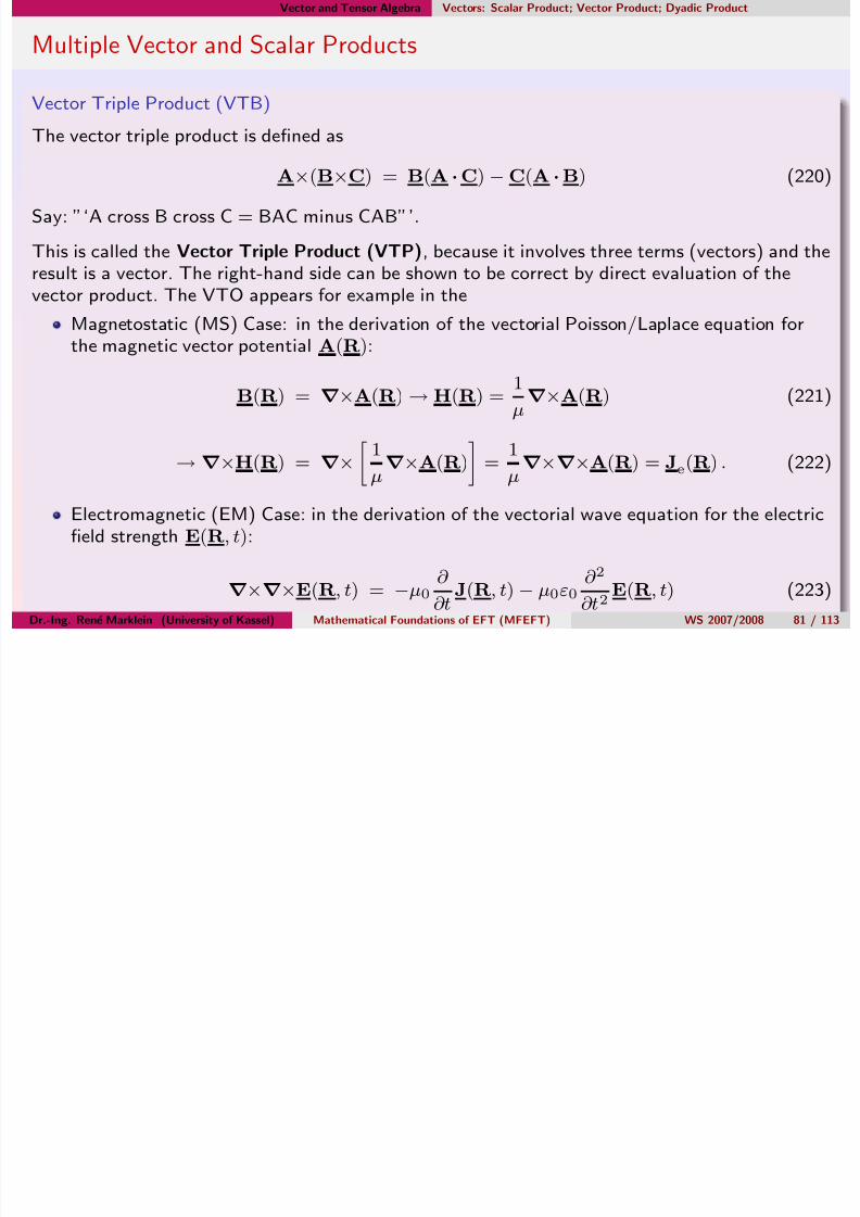
7/28/2019 lecture_p


The vector triple product is defined as

A×(B×C) = B(A ·C) −C(A ·B) (220)

Say: ”‘A cross B cross C = BAC minus CAB”’.

This is called the Vector Triple Product (VTP), because it involves three terms (vectors) and theresult is a vector. The right-hand side can be shown to be correct by direct evaluation of thevector product. The VTO appears for example in the

Magnetostatic (MS) Case: in the derivation of the vectorial Poisson/Laplace equation forthe magnetic vector potential A(R):

B(R) = ∇×A(R) → H(R) =1

µ∇×A(R) (221)

→∇×H(R) =

∇× 1

µ∇×A(R) =

1

µ∇×∇×A(R) = Je(R) . (222)

Electromagnetic (EM) Case: in the derivation of the vectorial wave equation for the electricfield strength E(R, t):

∇×∇×E(R, t) = −µ0∂

∂tJ(R, t)− µ0ε0

∂ 2

∂t2E(R, t) (223)




Proof of the Identity A×(B×C) = B(A ·C)−C(A ·B)

7/28/2019 lecture_p


B×C = ex ey ezBx By Bz

Cx Cy Cz

(225)

= (ByCz − BzCy)ex + (BzCx − BxCz)ey + (BxCy − ByCx)ez . (226)

A×(B×C) =

ex ey ezAx Ay Az

(ByCz − BzCy) (BzCx − BxCz) (BxCy − ByCx)

(227)

= (Ay(BxCy − ByCx) −Az(BzCx − BxCz))ex

+ (Az(ByCz − BzCy)− Ax(BxCy − ByCx))ey

+ (Ax(BzCx − BxCz)− Ay(ByCz − BzCy))ez (228)

= BxexAyCy − AyByCxex −AzBzCxex + BxexAzCz

+ ByeyAzCz −AzBzCyey −AxBxCyey + ByeyAxCx

+ BzezAxCx −AxBxCzez − AyByCzez + BzezAyCy . (229)





7/28/2019 lecture_p


A×(B×C)= BxexAyCy −AyByCxex − AzBzCxex + BxexAzCz

+ByeyAzCz −AzBzCyey −AxBxCyey + ByeyAxCx

+BzezAxCx −AxBxCzez − AyByCzez + BzezAyCy (230)

= Bxex (AyCy + AzCz)

−(AyBy + AzBz) Cxex

+ Byey (AzCz + AxCx)− (AzBz + AxBx) Cyey

+ Bzez (AxCx + AyCy)− (AxBx + AyBy) Czez (231)

= Bxex (AyCy + AzCz) +BxexAxCx − (AyBy + AzBz) Cxex−BxexAxCx

+ Byey (AzCz + AxCx) +ByeyAyCy − (AzBz + AxBx) Cyey−ByeyAyCy

+ Bzez (AxCx + AyCy) +Bz

ezAzCz − (AxBx + AyBy) Cz

ez−Bz

ezAzCz (232)

= Bxex (AxCx + AyCy + AzCz)− (BxAx + AyBy + AzBz) Cxex

+ Byey (AxCx+AyCy + AzCz)− (AxBx+ByAy + AzBz) Cyey

+ Bzez (AxCx + AyCy+AzCz)− (AxBx + AyBy+BzAz) Czez . (233)




7/28/2019 lecture_p



A×(B×C)

= Bxex (AxCx + AyCy + AzCz) =A ·C

− (BxAx + AyBy + AzBz) =A ·B

Cxex

+ Byey (AxCx+AyCy + AzCz) =A ·C −

(AxBx+ByAy + AzBz) =A ·B

Cyey

+ Bzez (AxCx + AyCy+AzCz) =A ·C

− (AxBx + AyBy+BzAz) =A ·B

Czez (234)

= Bxex (A ·C) + Byey (A ·C) + Bzez (A ·C)

− (A ·B) Cxex − (A ·B) Cyey − (A ·B) Czez (235)

= B (A ·C) − (A ·B)C . (236)




7/28/2019 lecture_p


Scalar Triple Product (STP)

The Scalar Triple Product is defined by

A · (B×C) = [ABC] , (237)

which determines the volume of the parallelepiped represented by the vectors A,B,C. Thisscalar value is a so-called Pseudo Scalar [Hafner , 1987], because the sign depends on the

handedness of the involved vector product.

Special Cases of the Scalar Triple Product (STP)

The resulting vector of two vectors is always perpendicular to both vectors, then

A · (A

×B) = 0

B · (A×B) = 0 . (238)



Dyadic Product

Definition of the Dyadic Product

7/28/2019 lecture_p


Definition of the Dyadic Product

The Dyadic Product (”‘product without a dot or cross”’) of two vectors is defined by the formal

multiplication of the vectors in components form

AB = (Axex + Ayey + Azez) (Bxex + Byey + Bzez) . (239)

The multiplication gives the dyadic products of the unit vectors:

AB = AxBxexex + AxByexey + AxBzexez

+AyBxeyex + AyByeyey + AyBzeyez

+AzBxezex + AzByezey + AzBzezez . (240)

The dyadic product is not commutative, this means

AB = BA

ex ey = ey ex

ex ez = ez ex

...



Dyadic Product

Dyadic Product in Matrix Form

W l i h f f h d di d i 3 3 M i Th ( i )

7/28/2019 lecture_p


We also can write the components form of the dyadic product in a 3×3 Matrix. The (cartesian)components representation of a vector

A = Axex + Ayey + Azez (241)

can be written by keeping the unit vectors in mind in form of a row vector or a column vector

{A} = {Ax Ay Az} (row vector) (242)

{A} = Ax

Ay

Az

(column vector) . (243)

Then, it follows for the dyadic product of two vectors AB by keeping the unit vectors of thefixed coordinate system in mind

AB = Ax

Ay

Az

{Bx By Bz} = AxBx AxBy AxBz

AyBx AyBy AyBz

AzBx AzBy AzBz

. (244)

Obviously, the dyadic products exiexj , i,j = 1, 2, 3, in Eq. (240) determine the position of the

AiBj element in the matrix in Eq. (244).



Dyadic Product


7/28/2019 lecture_p



The entry AxBz is positioned at the place exez

AB =

AxBx AxBy AxBz

AyBx AyBy AyBz

AzBx AzBy AzBz

and the entry AzBx is given by the position ezex

AB =

AxBx AxBy AxBz

AyBx AyBy AyBz

AzBx AzBy AzBz

.

This proves that the dyadic product is not commutative

AB

= BA . (245)

We summarize: In this sense, the dyad has nine ”‘components”’ in comparison to the the threecomponents of a vector. In the discussed case AB, these nine components are determined by sixvector components.



Dyadic Product

7/28/2019 lecture_p


Practical Meaning of the Dyadic Product

A practical meaning of the dyadic product, if — according to a matrix-vector multiplication — adot product (contraction) is a applied to a vector. We interpret the operation – the linearmapping —

AB ·C = AxBx AxBy AxBz

AyBx AyBy AyBz

AzBx AzBy AzBzCx

Cy

Cz (246)

or

C ·AB = {Cx Cy Cz}

AxBx AxBy AxBz

AyBx AyBy AyBz

AzBx AzBy AzBz

(247)

in a meaningful way.

Dr -Ing Rene Marklein (University of Kassel) Mathematical Foundations of EFT (MFEFT) WS 2007/2008 89 / 113


Dyadic Product


For example we find by computing the Dyad Vector Multiplication in Eq (246) and

7/28/2019 lecture_p


For example, we find by computing the Dyad–Vector Multiplication in Eq. (246) andinterpretation of the result according to Eq. (243)

AB ·C =

AxBxCx + AxByCy + AxBzCz

AyBxCx + AyByCy + AyBzCz

AzBxCx + AzByCy + AzBzCz

= Ax(BxCx + ByCy + BzCz)Ay(BxCx + ByCy + BzCz)Az(BxCx + ByCy + BzCz)

= (Axex + Ayey + Azez)(BxCx + ByCy + BzCz) (248)

and respectively by calculation of the Vector-Dyad Multiplication

C ·AB = (CxAx + CyAy + CzAz)(Bxex

+ Byey

+ Bzez

) , (249)

which can be written in the coordinate-free form

AB ·C = A(B ·C) (250)

C ·AB = (C ·A)B . (251)



Dyadic Product


7/28/2019 lecture_p


The result of the product of a dyad AB with a vector C

AB ·C = A(B ·C)

is again a vector, but in the direction of A, where the length is modified by the scalarproduct B ·Ca).

Similarly, the dot product of a vector C with a dyad AB

C ·AB = (C ·A)B

is a vector in direciton of B, which is stretched/compressed by the scalar product C ·A.

The contraction of a dyad with a vector determines a rotation of C in A or of C in B, where

AB ·C = C ·AB . (252)

a)Note that for all vectors C in a plane perpendicular to B is AB ·C = 0, i. e., the C’s are building the kernel of a(nullspace ) of the linear mapping AB ·C [Burg et al., 1990]; for all vectors in the kernel AB ·C = D it is impossible to solveC in a unique way.



EM Application: Hertzian Dipole Radiation

EM Application: Hertzian Dipole Radiation

7/28/2019 lecture_p


pp p

The simplest antenna to radiate electromagnetic waves is a Hertzian Dipole. The vector of theelectric field strength E of the radiated electromagnetic field is a function of the observationpoint R and has a different magnitude and direction at every point in space:

E(R, ω) = µ0 ω2 pe

(ω) ·G(0)(R, ω) . (253)

The change in direction (rotation) and amplitude (stretching/compression) relative to the

arbitrary but constant directed dipole moment pe is given by a dyad, the so-called DyadicGreen’s Function:

G(R, ω) =

I+

1

k20∇∇

e j k0R

4πR

= I− R R+j

k0R(I−

3R R)−

1

k20R2

(I−

3R R) e j k0R

4πRfor R

= 0

def = G(0)(R, ω) for R = 0 . (254)



Dyadic Product

7/28/2019 lecture_p


The Cross Product between a Vector and a Dyad

We can generalize the results obtained for the scalar product to the vector product of a vectorand a dyad and vice versa:

AB×C = A(B

×C)

(255)C×AB = (C×A)B , (256)

but note that the result is a dyad and these relations are not commutative.

Dr Ing Rene Marklein (University of Kassel) Mathematical Foundations of EFT (MFEFT) WS 2007/2008 93 / 113


Dyadic Product

Dyadic Product with Numbered Coordinates and Summation Convention

7/28/2019 lecture_p


y

If we use the numbered Cartesian coordinates (240) we write:

AB =3

i=1

3j=1

AxiBxjexiexj (257)

and applying the summation convention we find:

AB = Axi Bxj exi exj , (258)

where we have to sum i, j from 1, 2, 3. Note that exi exj = exj exi for i = j. A dyad AB has

components with double indices

Dxixj = Axi Bxj ; (259)

this results in the notation of a so-called 2nd rank tensor D:

D = AB = Axi Bxj exi exj = Dxixj exi exj . (260)



7/28/2019 lecture_p


Lecture 5: Complex Vectors; Tensors



MFEFT - Lecture 5

1 Introduction


7/28/2019 lecture_p


Position Vector and Coordinate SystemsCartesian Coordinates

Einstein’s Summation ConventionDifferentiation of the Position Vector; Kronecker Symbol (Kronecker Delta)Cylinder Coordinate SystemOrthogonal Curvilinear Coordinate SystemSpherical Coordinate SystemDupin Coordinates


TensorsDefinition


4 Distributions

5 Complex Analysis

6 Special Functions

7 Fourier Transform

8 Laplace Transform



Complex Vectors

7/28/2019 lecture_p


Definition of a Complex Vector

When we apply a Fourier Transformation with regard to time t the real valued electromagneticvector fields are changing to a complex valued frequency spectrum: We have to deal withcomplex vectors and their algebraic relations. A and B are two real vectors, this means vectorswith real components; we define then

C = A + jB (261)

as a Complex Vector C with the (Cartesian) components

Cx = Ax + j Bx

Cy = Ay + j By (262)

Cz = Az + j Bz

which are Complex Scalar Vector Components.



Complex Vectors

D fi iti f C j t C l V t d th H it S l P d t

7/28/2019 lecture_p


Definition of a Conjugate Complex Vector and the Hermite Scalar Product

With

C∗ = A− jB (263)

we mean a Conjugate Complex Vector C∗, and it is

C ·C = A2

−B2 + 2 jA ·B . (264)

With the Hermite Scalar Product

C ·C∗ = A2 + B2

= |Cx|2 + |Cy|2 + |Cz |2 (265)

we define the — positive real! — ”‘length”’ of C:

|C| = C ·C∗ . (266)



Complex Vectors

7/28/2019 lecture_p


Definition of a Complex Vector Product

Further, it is

C×C = 0 (267)

and

C×C∗ = 2 jB×A , (268)

i. e., the vector product C×C∗ is equal zero, if A and B are parallel.

D Ing R n´ M kl in (Uni sit f K ss l) M th m ti l F nd ti ns f EFT (MFEFT) WS 2007/2008 99 / 113

7/28/2019 lecture_p


Vector and Tensor Algebra Tensors

Tensors

7/28/2019 lecture_p


Row and Column Vectors of a Tensor of 2nd Rank: Dyad

With the row vectors

Dxi= Dxi xj exj (271)

and column vectors

D

xj

= Dxixj exi (272)

we can write D as a sum over the following dyadic productsa:

D = exiDxi(273)

= Dxj exj . (274)

aIn the dyad AB is the i–th row vector Axi B and the j-th column vector BxjA.

D I R ´ M kl i (U i it f K l) M th ti l F d ti f EFT (MFEFT) WS 2007/2008 101 / 113

Vector and Tensor Analysis

MFEFT - Outline

1 Introduction


7/28/2019 lecture_p


yCartesian Coordinates


Vectors: Scalar Product; Vector Product; Dyadic ProductScalar ProductVector Product

Dyadic ProductComplex Vectors

TensorsDefinition


4 Distributions

5 Complex Analysis6 Special Functions

7 Fourier Transform

8 Laplace Transform

D I R ´ M kl i (U i it f K l) M th ti l F d ti f EFT (MFEFT) WS 2007/2008 102 / 113



7/28/2019 lecture_p


D I R ´ M kl i (U i i f K l) M h i l F d i f EFT (MFEFT) WS 2007/2008 103 / 113

Distributions

MFEFT - Outline

1 Introduction


7/28/2019 lecture_p


Cartesian Coordinates




TensorsDefinition


4 Distributions


7 Fourier Transform

8 Laplace Transform


Distributions

Distributions

7/28/2019 lecture_p



Complex Analysis

MFEFT - Outline

1 Introduction


C t i C di t

7/28/2019 lecture_p






TensorsDefinition


4 Distributions


7 Fourier Transform

8 Laplace Transform


Complex Analysis

Complex Analysis

7/28/2019 lecture_p



Special Functions

MFEFT - Outline

1 Introduction



7/28/2019 lecture_p






TensorsDefinition


4 Distributions


7 Fourier Transform

8 Laplace Transform


Special Functions

Special Functions

7/28/2019 lecture_p



Fourier Transform

MFEFT - Outline

1 Introduction



7/28/2019 lecture_p






TensorsDefinition


4 Distributions


7 Fourier Transform

8 Laplace Transform


Fourier Transform

Fourier Transform

7/28/2019 lecture_p



Laplace Transform

MFEFT - Outline

1 Introduction



7/28/2019 lecture_p





TensorsDefinition


4 Distributions


7 Fourier Transform

8 Laplace Transform


Laplace Transform

Laplace Transform

7/28/2019 lecture_p



lecture_p

Documents