1

In the Name of God

Lectures 15&16: Radial Basis Function Networks

Some Historical Notes

• Learning is equivalent to finding a surface in a multidimensional space that provides a best fit to themultidimensional space that provides a best fit to the training data.

• Cover (1965): A pattern-classification problem cast in a high-dimensional space is more likely to be linearlyhigh dimensional space is more likely to be linearly separable than in a low-dimensional space.

• Powell (1985): Radial-basis functions were introduced in the solution of the real multivariate interpolation problem.the solution of the real multivariate interpolation problem.

• Broomhead and Lowe (1988) were the first to exploit the use of radial-basis functions in the design of neural networks.

• Mhaskar, Niyogi and Girosi (1996): The dimension of the hidden space is directly related to the capacity of the network to approximate a smooth input-output mapping (th hi h th di i f th hidd th(the higher the dimension of the hidden space, the more accurate the approximation will be).

Radial-Basis Function NetworksRadial Basis Function Networks• In its most basic form Radial-Basis Function

(RBF) network involves three layers with entirely different roles.▫ The input layer is made up of source nodes that

connect the network to its environment.▫ The second layer the only hidden layer applies▫ The second layer, the only hidden layer, applies

a nonlinear transformation from the input space to the hidden space. p

▫ The output layer is linear, supplying the response of the network to the activation pattern applied to th i t lthe input layer.

Radial-Basis Function NetworksRadial Basis Function Networks• They are Feedforward neural networksy▫ compute activations at the hidden neurons using

an exponential of a [Euclidean] distance measure b t th i t t d t t tbetween the input vector and a prototype vectorthat characterizes the signal function at a hidden neuron.neuron.

• Originally introduced into the literature for the purpose of interpolation of data points on a p p p pfinite training set

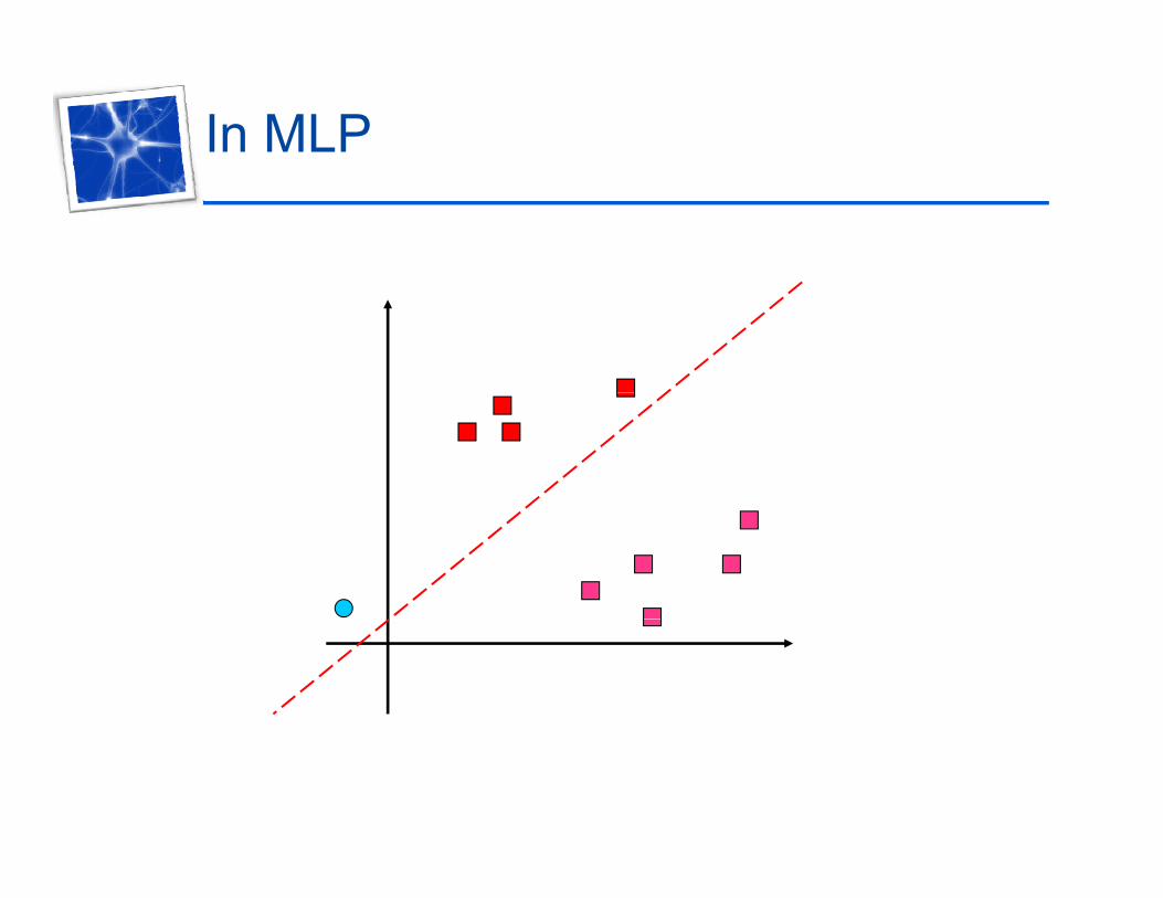
In MLP

In RBFN

Architecture

x1h1

h2W1

x2

x3

2

h3f(x)

W2

W3

xnhm

f(x)

Wm

Input layer Hidden layer Output layer

Three layers

• Input layerp y▫ Source nodes that connect to the network of its

environmentHidd l• Hidden layer▫ Hidden units provide a set of basis functions▫ High dimensionalityHigh dimensionality

• Output layer▫ Linear combination of hidden functions

Linear Models

• A linear model for a function f(x) takes the form:

• The model f(.) is expressed as a linear combination of a set of m basis functions. • The freedom to choose different values for the• The freedom to choose different values for the weights, derives the flexibility of f(.), its ability to fit many different functions. • Any set of functions can be used as the basis set, however, models containing only basis functions drawn from one particular class have a special interestfrom one particular class have a special interest.• h(x) is mostly Gaussian function

Special Base Functions

• Classical statistics - polynomials base functions:

• Signal processing applications - combinations of sinusoidal waves (Fourier series):of sinusoidal waves (Fourier series):

• Artificial neural networks (particularly in multi-layer perceptrons) - logistic functions:

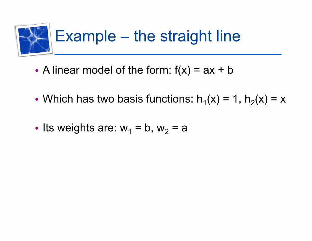
Example – the straight lineg

• A linear model of the form: f(x) = ax + b ( )

• Which has two basis functions: h1(x) = 1, h2(x) = x

• Its weights are: w1 = b, w2 = a

Radial FunctionsRadial Functions• Characteristic feature - their response

d ( i ) t i ll ithdecreases (or increases) monotonically with distance from a central point.

• The center, the distance scale, and the , ,precise shape of the radial function are parameters of the model, all fixed if it is linearlinear.

• Typical radial functions are:▫ The Gaussian RBF (monotonically decreases with

distance from the center)distance from the center).▫ A multiquadric RBF (monotonically increases with

distance from the center).

Radial functionsRadial functions

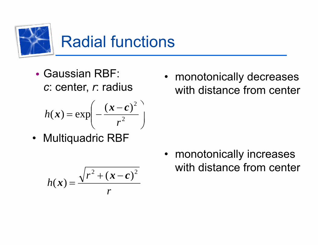
• Gaussian RBF: • monotonically decreasesGaussian RBF:c: center, r: radius

2)( cx

• monotonically decreases with distance from center

2

)(exp)(r

h cxx

• Multiquadric RBF• Multiquadric RBF• monotonically increases

with distance from center

rr

h22 )(

)(cx

x

with distance from center

Radial Functions

G i RBF lti d i RBFGaussian RBF multiqradric RBF

Cover’s Theorem

“A complex pattern-classification problem cast in high-dimensional space nonlinearly is more likely to be linearly separable than in amore likely to be linearly separable than in a low dimensional space”

(Cover 1965)(Cover, 1965)

Introduction to Cover’s Theorem

• Let X denote a set of N patterns (points) x1, x2, p (p ) 1, 2,x3, …, xN

• Each point is assigned to one of two classes: X+

and X-

• This dichotomy is separable if there exists a f th t t th t l fsurface that separates these two classes of

points.

Introduction to Cover’s Theorem

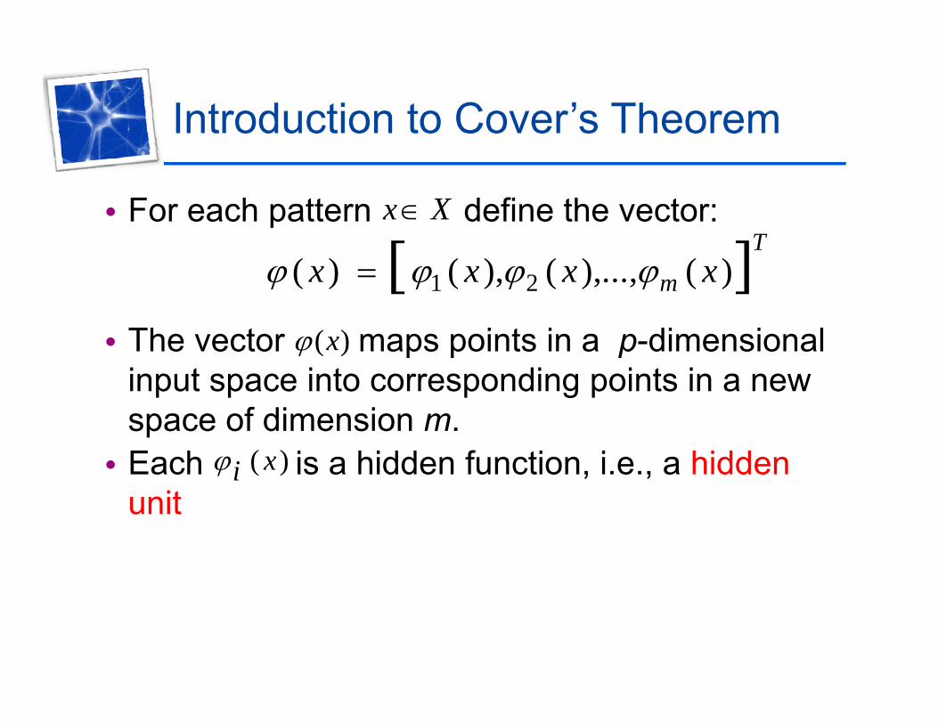
• For each pattern define the vector:Xxp

1 2( ) ( ), ( ),..., ( )T

mx x x x

• The vector maps points in a p-dimensional input space into corresponding points in a new

f di i

)(x

space of dimension m.• Each is a hidden function, i.e., a hidden

unit( )xi

unit

Introduction to Cover’s TheoremIntroduction to Cover s Theorem

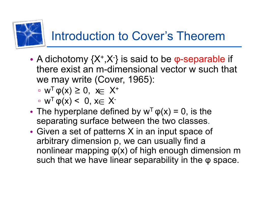
• A dichotomy {X+,X-} is said to be φ-separable if there exist an m-dimensional vector w such that we may write (Cover, 1965):▫ wTφ(x) ≥ 0 x X+▫ wTφ(x) ≥ 0, x X▫ wTφ(x) < 0, x X-

• The hyperplane defined by wTφ(x) = 0, is the

separating surface between the two classes.• Given a set of patterns X in an input space of

arbitrary dimension p we can usually find aarbitrary dimension p, we can usually find a nonlinear mapping φ(x) of high enough dimension m such that we have linear separability in the φ space.

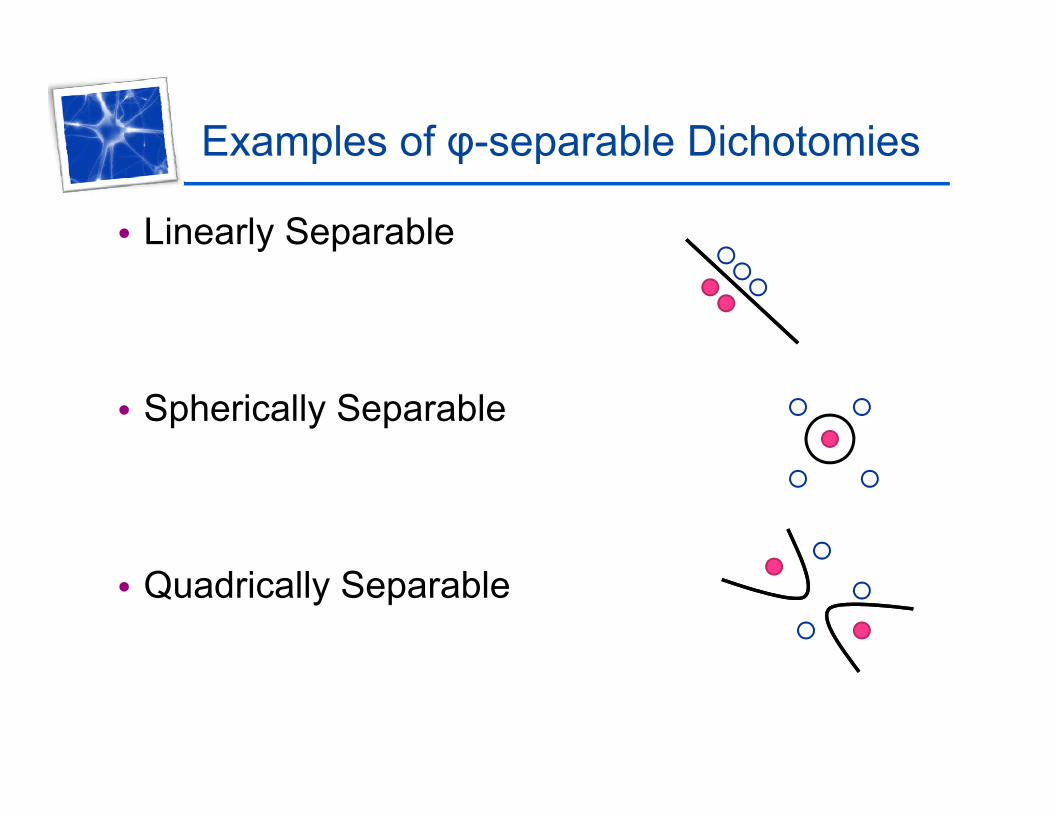
Examples of φ-separable DichotomiesExamples of φ separable Dichotomies

• Linearly Separable

• Spherically Separable

• Quadrically Separable

Back to the XOR Problem

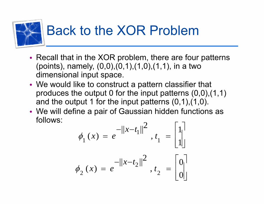
• Recall that in the XOR problem, there are four patterns ( i t ) l (0 0) (0 1) (1 0) (1 1) i t(points), namely, (0,0),(0,1),(1,0),(1,1), in a two dimensional input space.

• We would like to construct a pattern classifier that produces the output 0 for the input patterns (0,0),(1,1) and the output 1 for the input patterns (0,1),(1,0).

• We will define a pair of Gaussian hidden functions as pfollows:

11 1

2|| || 1( ) ,

1x t

x e t 1 1 1

22|| || 0

( )x t

t 2

2 2( ) ,0

x e t

Back to the XOR Problem

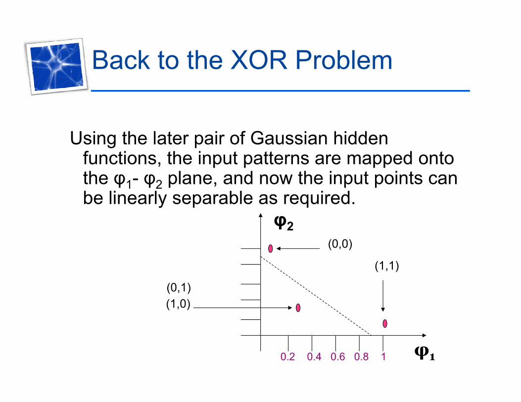
Using the later pair of Gaussian hidden functions, the input patterns are mapped onto the φ φ plane and now the input points canthe φ1- φ2 plane, and now the input points can be linearly separable as required.

φ2φ2(0,0)

(1,1)

(0,1)(1,0)

0.2 0.4 0.6 0.8 1 φ1

Interpolation Problem

• Assume a domain X and a range Y taken to be metric

• Existence: For every input vector x H, there does exist an output range Y taken to be metric

space, and that is related by a fixed but unknown mapping f.

• The problem of

, py=f(x), where y H .

• Uniqueness: For any pair of input vectors x,t H, we have f(x)=f(t) if, and only if x=t.• The problem of

reconstructing the mapping f is said to be well-posed if three conditions are satisfied:

f(x) f(t) if, and only if x t.• Continuity: (=stability) for any

>0 there exists =() such that the condition x(x,t)< implies that (f(x) f(t))< where ( ) issatisfied: that y(f(x),f(t))<, where (.,.) is the symbol for distance between the two arguments in their respective spaces.

Interpolation Problem

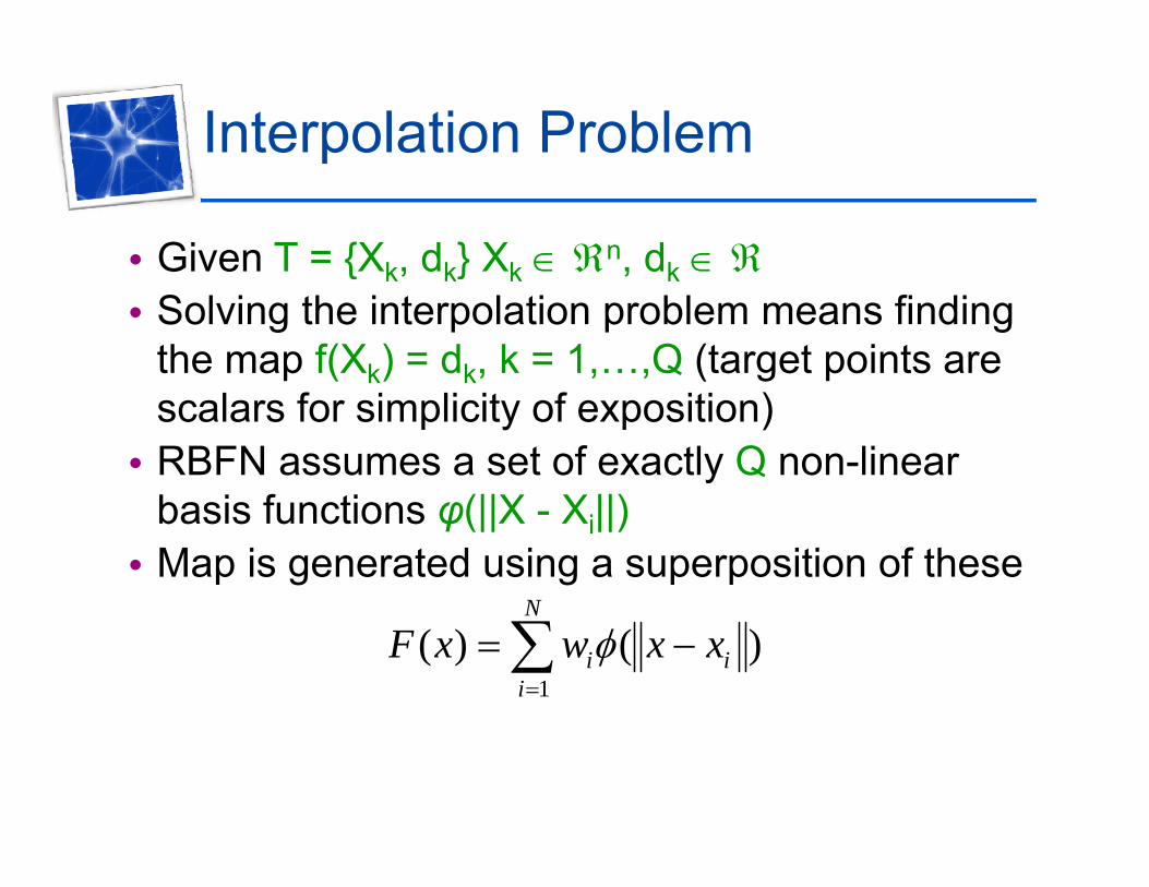
• Given T = {Xk, dk} Xk n, dk { k, k} k , k• Solving the interpolation problem means finding

the map f(Xk) = dk, k = 1,…,Q (target points are scalars for simplicity of exposition)

• RBFN assumes a set of exactly Q non-linear b i f ti (||X X ||)basis functions φ(||X - Xi||)

• Map is generated using a superposition of theseN

1( ) ( )

N

i ii

F x w x x

Application of Interpolation in Signal ProcessingProcessing

Converting digital signals to continuous signal

Up-sampling

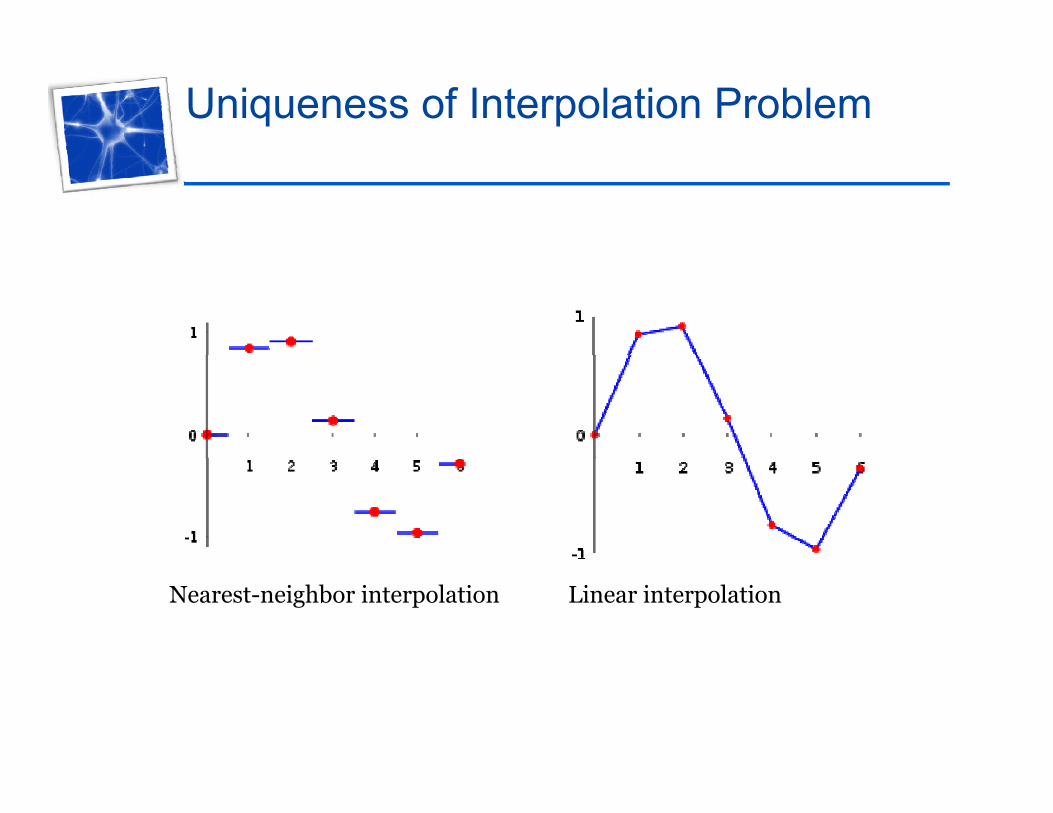
Uniqueness of Interpolation Problem

Nearest-neighbor interpolation Linear interpolation

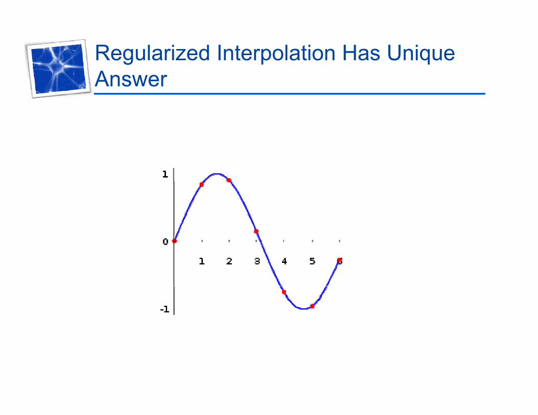
Regularized Interpolation Has Unique AnswerAnswer

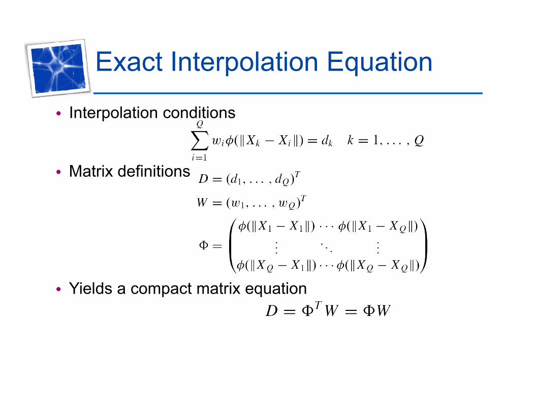
Exact Interpolation Equation

• Interpolation conditions

• Matrix definitions

Yi ld t t i ti• Yields a compact matrix equation

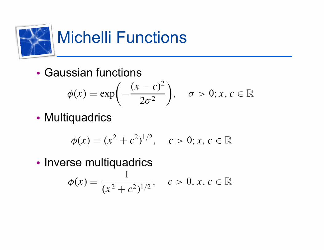
Michelli Functions

• Gaussian functions

• Multiquadrics

• Inverse multiquadrics

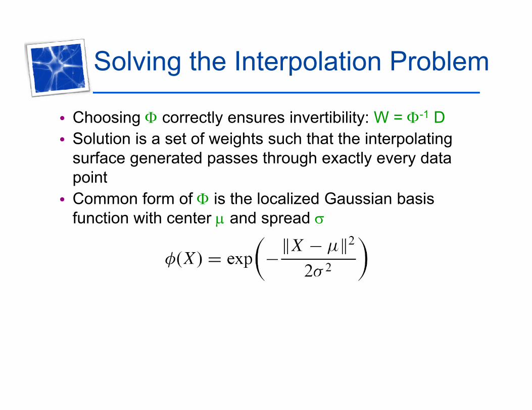
Solving the Interpolation Problemg

• Choosing correctly ensures invertibility: W = -1 D• Solution is a set of weights such that the interpolating

surface generated passes through exactly every data pointpoint

• Common form of is the localized Gaussian basis function with center and spread

Radial Basis Function Network

1x1

2x2

Qxn

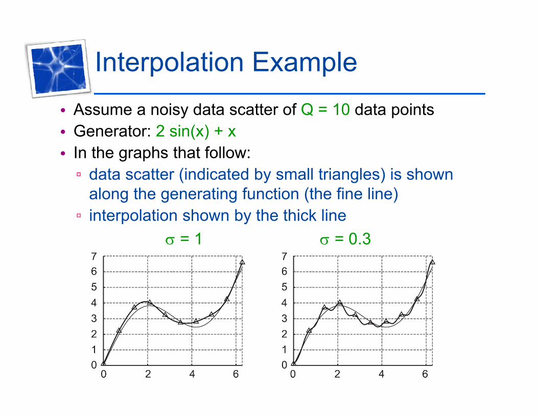
Interpolation Example• Assume a noisy data scatter of Q = 10 data points

Generator: 2 sin(x) + x• Generator: 2 sin(x) + x• In the graphs that follow:▫ data scatter (indicated by small triangles) is shown ( y g )

along the generating function (the fine line)▫ interpolation shown by the thick line

1 0 3 = 1 = 0.3

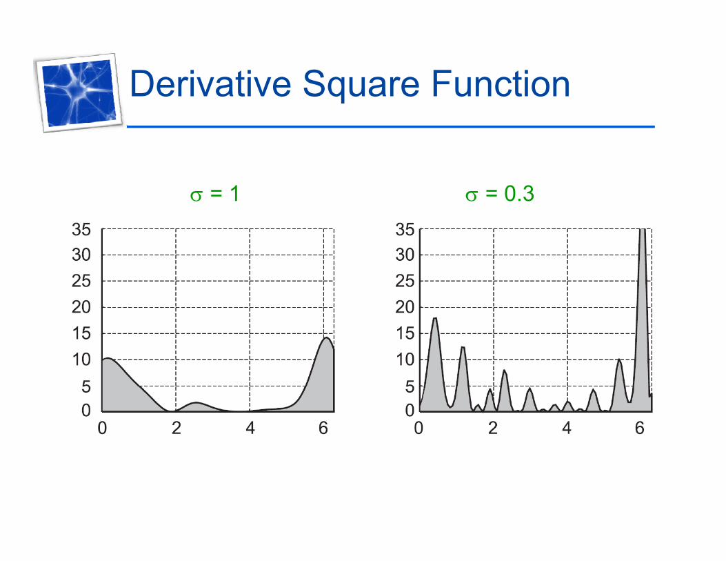
Derivative Square Function

= 1 = 0.3

Notes

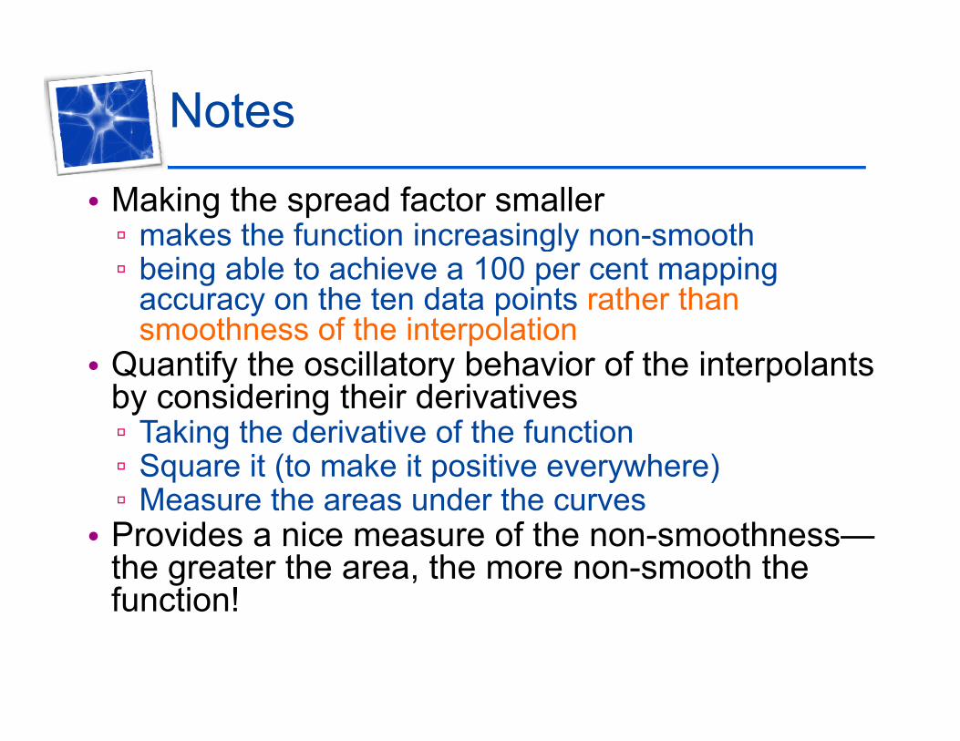
• Making the spread factor smallermakes the function increasingly non smooth▫ makes the function increasingly non-smooth

▫ being able to achieve a 100 per cent mapping accuracy on the ten data points rather than smoothness of the interpolationsmoothness of the interpolation

• Quantify the oscillatory behavior of the interpolantsby considering their derivatives ▫ Taking the derivative of the function▫ Square it (to make it positive everywhere) ▫ Measure the areas under the curves

• Provides a nice measure of the non-smoothness—the greater the area, the more non-smooth the function!function!

Problems

• Oscillatory behavior is highly undesirable for proper generalization

• Better generalization is achievable with smoother functions which are fitted to noisy datafunctions which are fitted to noisy data

• Number of basis functions in the expansion is equal to the number of data points!▫ Not possible to have for real-world datasets, which

can be extremely large▫ Computational and storage requirements for them▫ Computational and storage requirements for them

can explode very quickly

The RBFN Solution• Choose the number of basis functions to be some

number q < Qnumber q Q• No longer restrict the centers of the basis functions to

be fixed to the data point values. ▫ Now made trainable parameters of the model

• Spreads of each of the basis functions is permitted to be different and trainable. ▫ Learning can be done either by supervised or

unsupervised techniquesunsupervised techniques• A bias is included in the final linear superposition• Assume centers and spreads of the basis functions are

optimized and fixedoptimized and fixed• Proceed to determine the hidden–output neuron

weights using the procedure adopted in the interpolation casecase

Solving the Problem in a Least Squares SenseSquares Sense

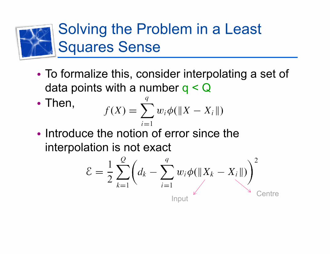
• To formalize this, consider interpolating a set of , p gdata points with a number q < Q

• Then,

• Introduce the notion of error since the i t l ti i t tinterpolation is not exact

CentreInput

Compute the Optimal Weightsg

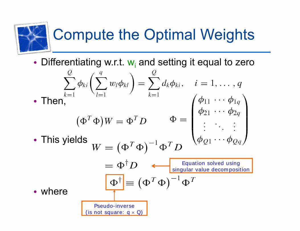
• Differentiating w.r.t. wi and setting it equal to zero

• Then• Then,

• This yields

h

Equation solved usingsingular value decomposition

• wherePseudo-inverse

(is not square: q Q)

More generalizationg• Straightforward to include a bias term w0 into the

approximation equationapproximation equation

• Basis function is generally chosen to be the Gaussian

• RBFs can be generalized to include arbitrary covariance matrices Ki

• Universal approximator• RBFNs have the best approximation property

▫ The set of approximating functions that RBFNs are capable of▫ The set of approximating functions that RBFNs are capable of generating, there is one function that has the minimum approximation error for any given function which has to be approximated

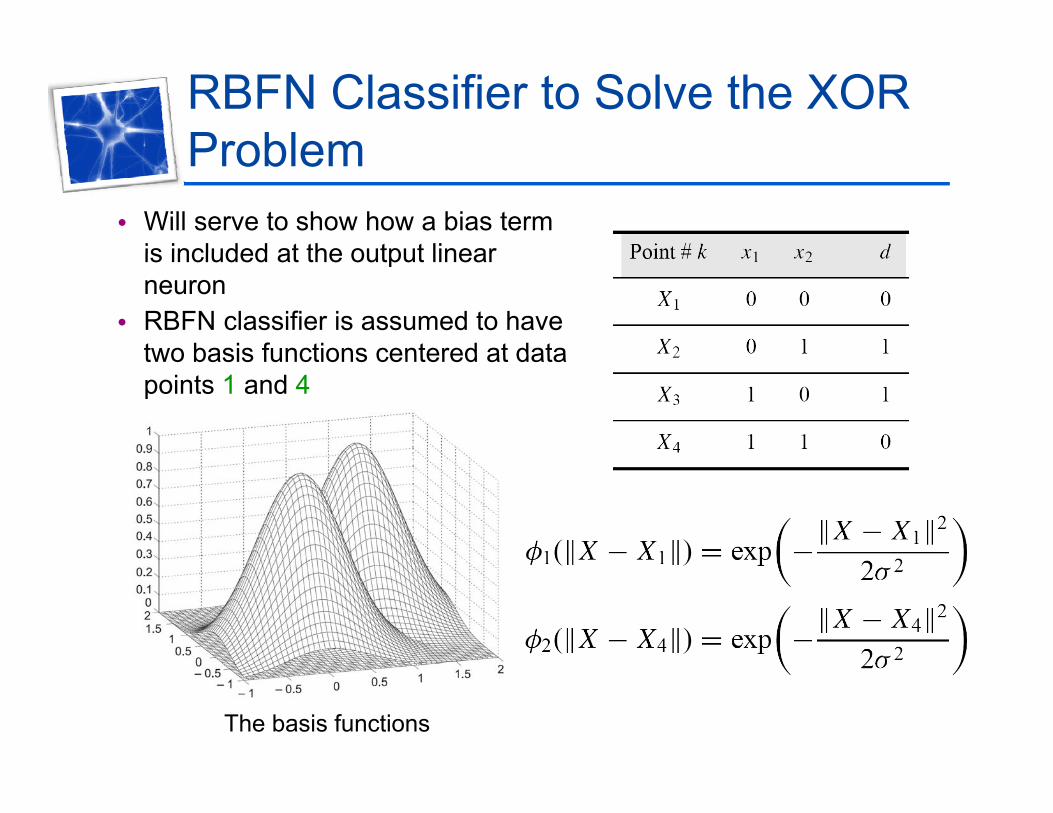
RBFN Classifier to Solve the XOR ProblemProblem

• Will serve to show how a bias term is included at the output linearis included at the output linear neuron

• RBFN classifier is assumed to have two basis functions centered at datatwo basis functions centered at data points 1 and 4

The basis functions

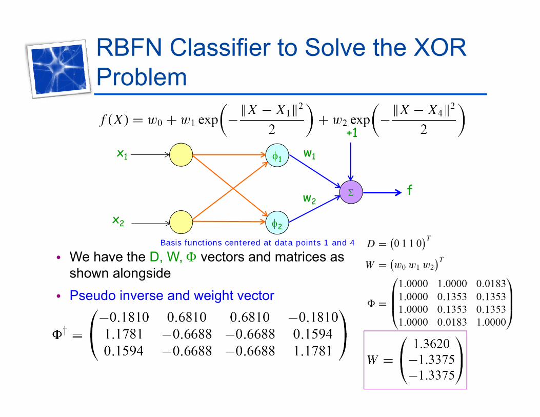
RBFN Classifier to Solve the XOR Problem

1

Problem

+1

1 w1x1

2

fw2

x2

Basis functions centered at data points 1 and 4

• We have the D, W, vectors and matrices as shown alongside

• Pseudo inverse and weight vector

Ill-Posed and Well-Posed Problems

• Ill-posed problems originally identified by Hadamard in th t t f ti l diff ti l tithe context of partial differential equations.

• Problems are well-posed if their solutions satisfy three conditions:▫ they exist▫ they are unique▫ they depend continuously on the data sety p y

• Problems that are not well-posed are ill-posed• Example▫ differentiation is an ill-posed problem because somedifferentiation is an ill posed problem because some

solutions need not depend continuously on the data▫ inverse kinematics problem which maps external real-world

movements into an internal coordinate system is also an ill-movements into an internal coordinate system is also an illposed problem

Approximation Problem is Ill-Posed

• The solution to the problem is not uniqueS ffi i t d t i t il bl t t t th• Sufficient data is not available to reconstruct the mapping uniquely

• Data points are generally noisyThe solution to the ill posed approximation problem lies• The solution to the ill-posed approximation problem lies in regularization▫ essentially requires the introduction of certain constraints that

impose a restriction on the solution spacep p• Necessarily problem dependent• Regularization techniques impose smoothness

constraints on the approximating set of functions• Some degree of smoothness is necessary for the

representative function since it has to be robust against noise

Regularization Theoryg y

• Assume training data T generated by random sampling f th f tiof the function

• Regularization techniques replace the standard error minimization problem with minimization of a regularization risk functional

• The main idea behind regularization is to stabilize the solution by means of prior informationy p

• This is done by including a function in the cost function• Only a small number of candidate solutions will minimize

this functionalthis functional• These functional terms are called the regularization

termsTypically the functional measure for the smoothness of• Typically, the functional measure for the smoothness of the function

Tikhonov Functional• Regularization risk functional comprises two terms

error function smoothness functional

i t iti l li t id i f ti d i ti t h t i th

• The smoothness functional is expressed as▫ P is a linear differential operator, ||·|| is a norm

intuitively appealing to consider using function derivatives to characterize smoothness

s a ea d e e t a ope ato , || || s a o• The regularization risk functional to be minimized is

regularization parameter

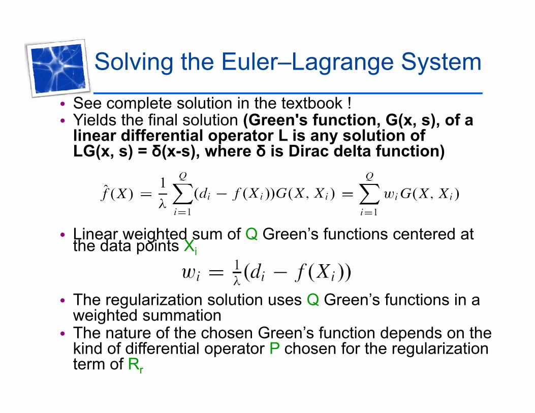
Solving the Euler–Lagrange System• See complete solution in the textbook !• Yields the final solution (Green's function, G(x, s), of a ( ( )

linear differential operator L is any solution of LG(x, s) = δ(x-s), where δ is Dirac delta function)

• Linear weighted sum of Q Green’s functions centered at• Linear weighted sum of Q Green s functions centered at the data points Xi

• The regularization solution uses Q Green’s functions in a weighted summation

• The nature of the chosen Green’s function depends on theThe nature of the chosen Green s function depends on the kind of differential operator P chosen for the regularization term of Rr

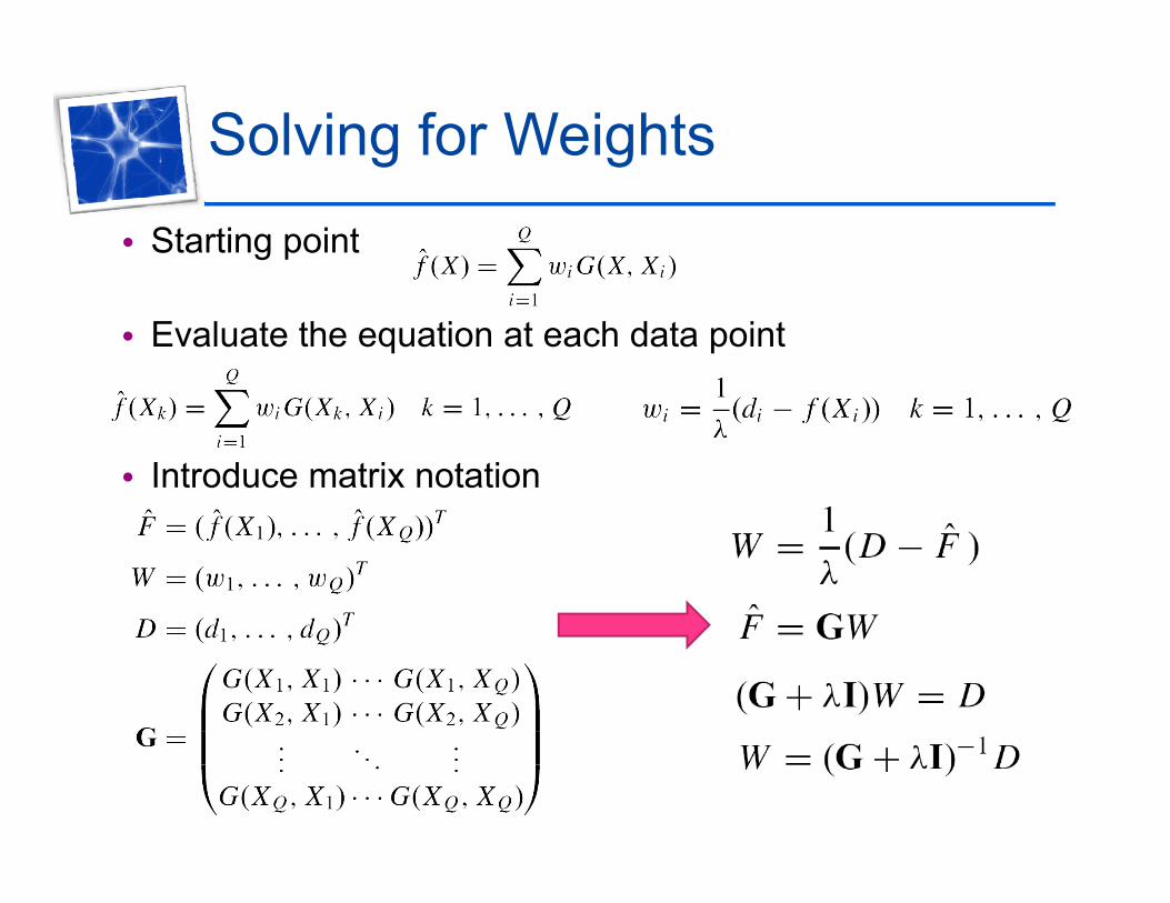
Solving for Weightsg g• Starting point

• Evaluate the equation at each data point

• Introduce matrix notation

Euclidean Norm Dependence

• If the differential operator P is p▫ rotationally invariant▫ translationally invariantTh h G ’ f i G(X Y) d d l• Then, the Green’s function G(X,Y) depends only on the Euclidean norm of the difference of the vectorsvectors

• Then• Then,

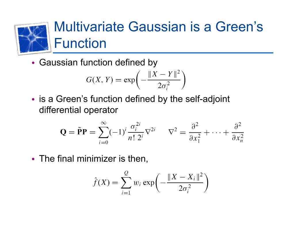
Multivariate Gaussian is a Green’s FunctionFunction

• Gaussian function defined by

• is a Green’s function defined by the self-adjointy jdifferential operator

• The final minimizer is then,The final minimizer is then,

Desirable Properties of Regularization NetworksNetworks

• The regularization network is a universal gapproximator, that can approximate any multivariate continuous function arbitrarily well,given sufficiently large number of hidden units.

• The approximation shows the best i ti t (b t ffi i t illapproximation property (best coefficients will

be found).• The solution is optimal: it will minimize the cost• The solution is optimal: it will minimize the cost

functional ( ).F

Generalized Radial Basis Function NetworkNetwork

• We now proceed to generalize the RBFN in two p gsteps▫ Reduce the Number of Basis Functions, Use

Non-Data Centers▫ Use a Weighted Norm

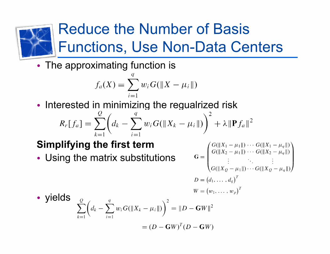
Reduce the Number of Basis Functions Use Non Data CentersFunctions, Use Non-Data Centers

• The approximating function is

• Interested in minimizing the regualrized risk

Simplifying the first termSimplifying the first term• Using the matrix substitutions

• yields

Reduce the Number of Basis Functions Use Non Data CentersFunctions, Use Non-Data Centers

Simplifying the second term• Use the properties of the adjoint of the differential

operator and Green’s function

• where

Fi ll• Finally

• And the optimal weights W are obtained asp g

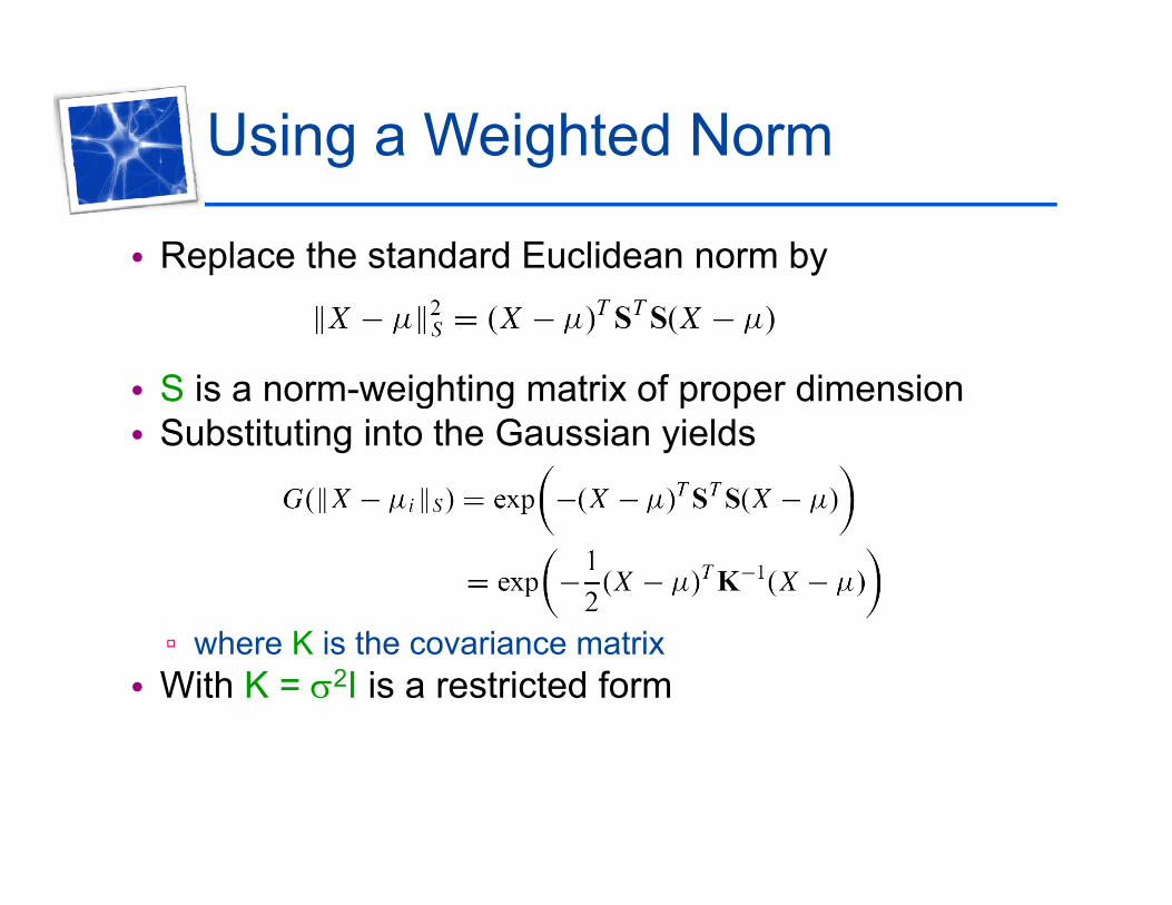
Using a Weighted Normg g

• Replace the standard Euclidean norm by

• S is a norm-weighting matrix of proper dimensionS is a norm weighting matrix of proper dimension• Substituting into the Gaussian yields

▫ where K is the covariance matrix• With K = 2I is a restricted form

Generalized Radial Basis Function NetworkNetwork

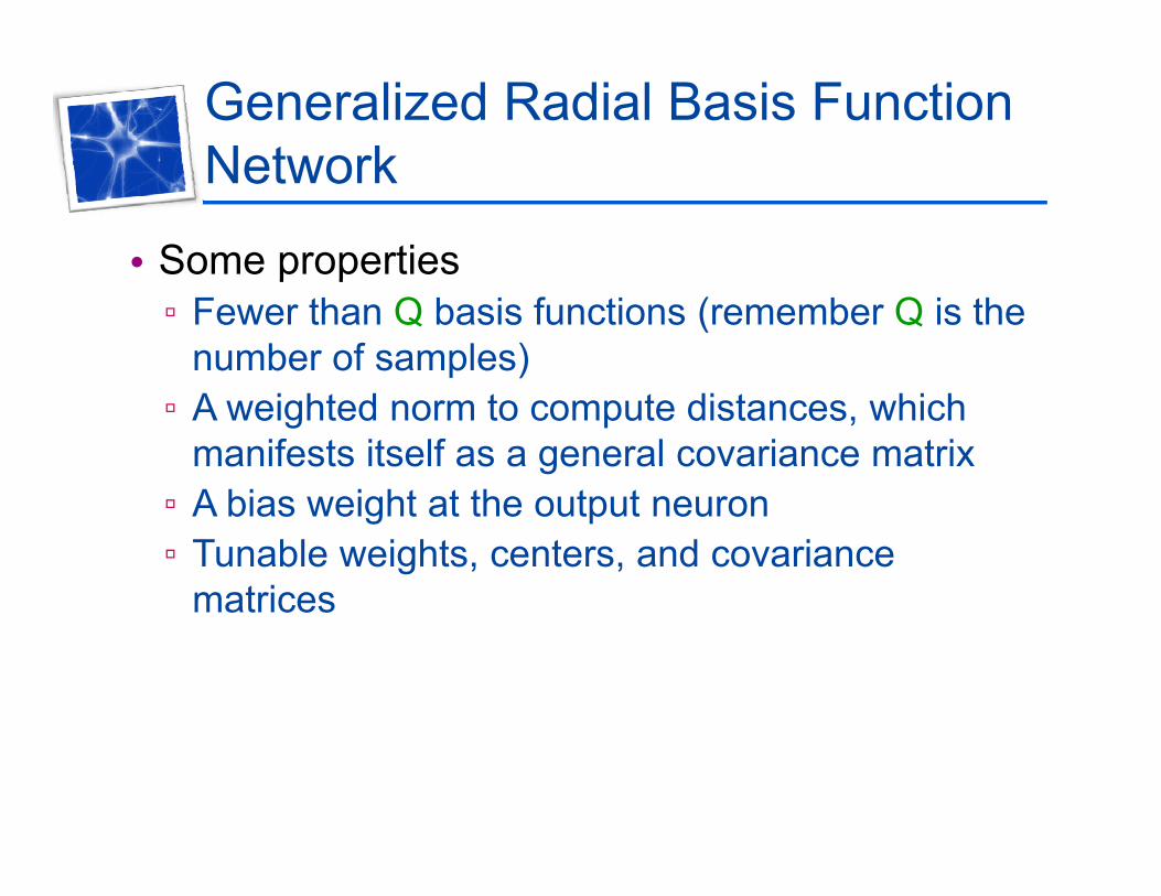
• Some propertiesp p▫ Fewer than Q basis functions (remember Q is the

number of samples)▫ A weighted norm to compute distances, which

manifests itself as a general covariance matrix▫ A bias weight at the output neuron▫ A bias weight at the output neuron▫ Tunable weights, centers, and covariance

matrices

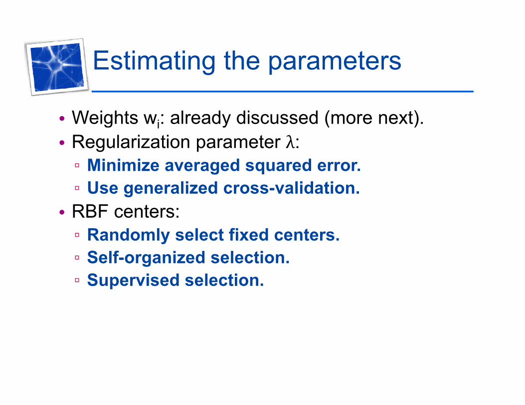
Estimating the parametersg

• Weights wi: already discussed (more next).g i y ( )• Regularization parameter :▫ Minimize averaged squared error.▫ Use generalized cross-validation.

• RBF centers:f▫ Randomly select fixed centers.

▫ Self-organized selection.▫ Supervised selection▫ Supervised selection.

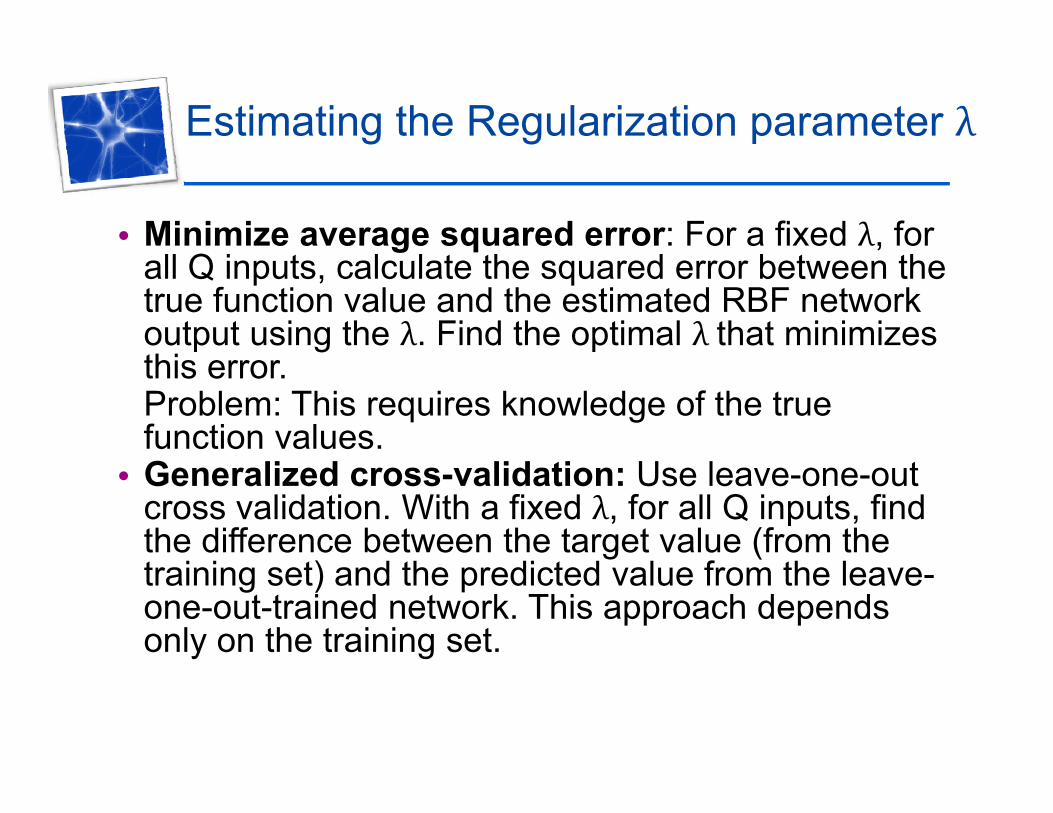
Estimating the Regularization parameter

• Minimize average squared error: For a fixed , for all Q inputs, calculate the squared error between the true function value and the estimated RBF network output using the . Find the optimal that minimizes thithis error.Problem: This requires knowledge of the true function values.

• Generalized cross-validation: Use leave-one-out cross validation. With a fixed , for all Q inputs, find the difference between the target value (from the

) ftraining set) and the predicted value from the leave-one-out-trained network. This approach depends only on the training set.

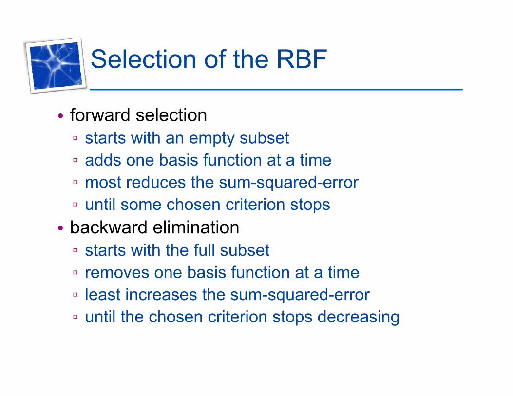
Selection of the RBF

• forward selection▫ starts with an empty subset▫ adds one basis function at a time▫ most reduces the sum-squared-error▫ until some chosen criterion stopsb k d li i ti• backward elimination▫ starts with the full subset▫ removes one basis function at a time▫ removes one basis function at a time▫ least increases the sum-squared-error▫ until the chosen criterion stops decreasingp g

Number of radial basis neurons

• By designery g• Max of neurons = number of patterns• Min of neurons = ( experimentally determined)• More neurons▫ More complex, but smaller tolerance

Learning strategies

• Two levels of Learningg▫ Center and spread learning (or determination)▫ Output layer Weights LearningM k # ( ) ll ibl• Make # ( parameters) as small as possible▫ Principles of Dimensionality

Various learning strategies

• how the centers of the radial-basis functions of the network are specified.

1. Fixed centers selected at random2. Self-organized selection of centers 3 Supervised selection of centers3. Supervised selection of centers

Fixed centers selected at random

• Fixed RBFs of the hidden units• The locations of the centers may be chosen

randomly from the training dataset• We can use different values of centers and

widths for each radial basis function -> i t ti ith t i i d t i d dexperimentation with training data is needed

Fixed centers selected at random

• Only output layer weight is needed to be learnedy p y g• Obtain the value of the output layer weight by

pseudo-inverse method• Main problem▫ Requires a large training set for a satisfactory level of

performanceperformance

Self-organized selection of centers

• Hybrid learningy g▫ self-organized learning to estimate the centers of

RBFs in hidden layeri d l i t ti t th li i ht f▫ supervised learning to estimate the linear weights of

the output layer• Self-organized learning of centers by means ofSelf organized learning of centers by means of

clustering• Supervised learning of output weights by LMS

algorithm (pseudo-inverse method)

Self-organized selection of centers

k-means clusteringg

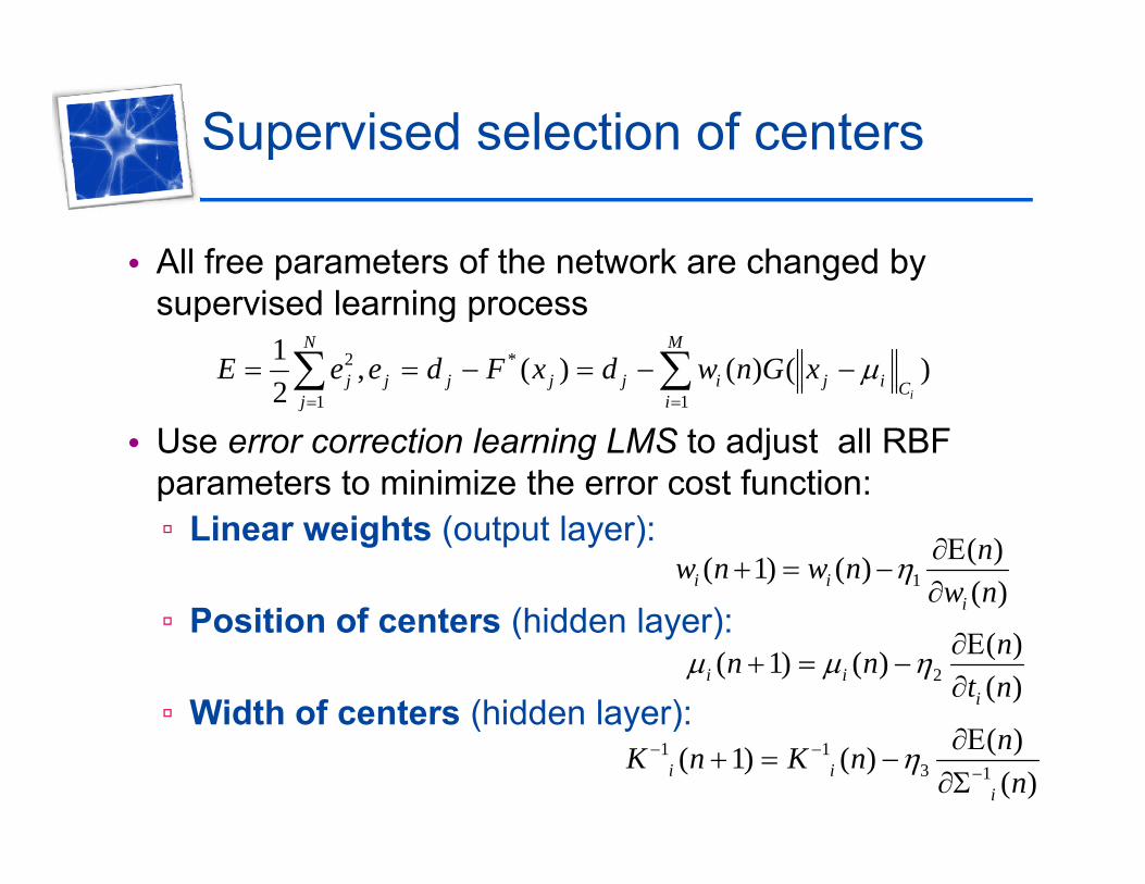
Supervised selection of centers

• All free parameters of the network are changed by p g ysupervised learning process

2 *1 , ( ) ( ) ( )2

N M

j j j j j i j i CE e e d F x d w n G x

• Use error correction learning LMS to adjust all RBF parameters to minimize the error cost function:

1 12 ij j j j j i j i C

j i

p▫ Linear weights (output layer):

P iti f t (hidd l )1

( )( 1) ( )( )i i

i

nw n w nw n

▫ Position of centers (hidden layer):

▫ Width of centers (hidden layer):

i

2( )( 1) ( )( )i i

i

nn nt n

Width of centers (hidden layer):

1 13 1

( )( 1) ( )( )i i

i

nK n K nn

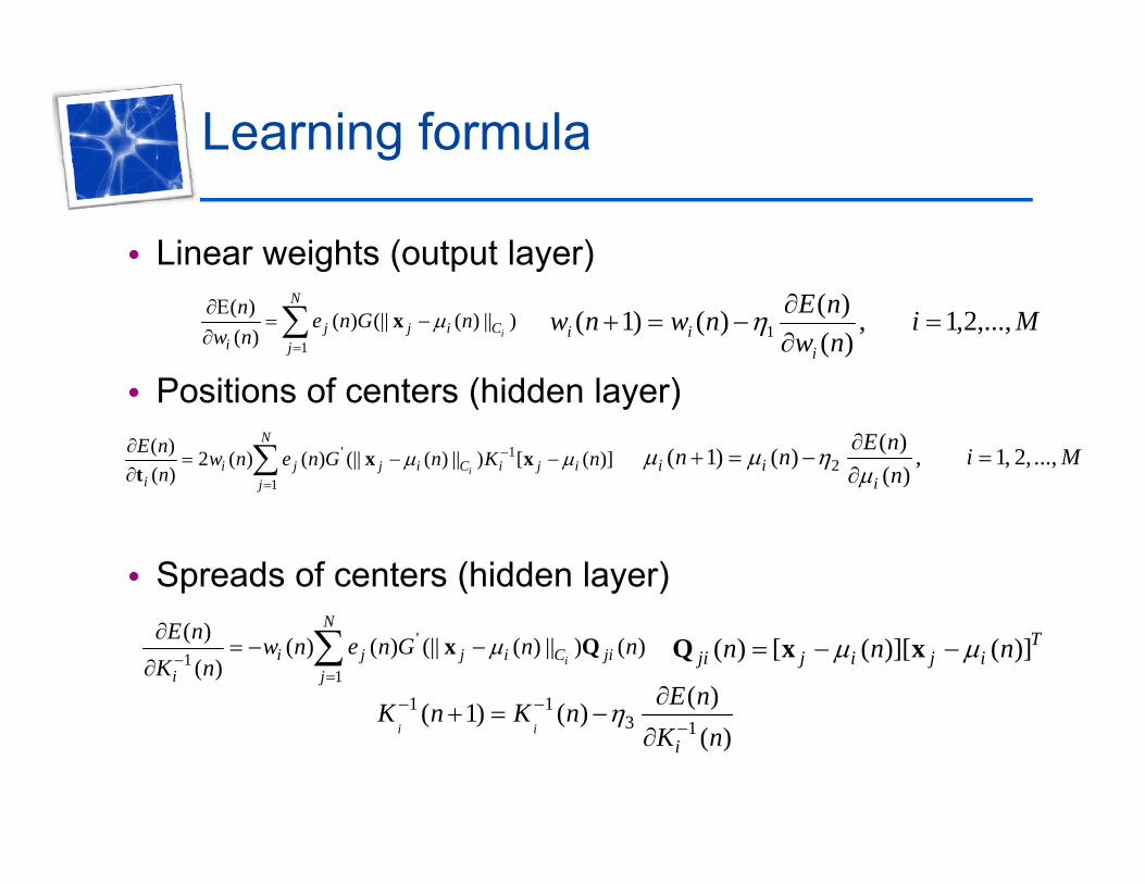
Learning formula

• Linear weights (output layer)

Positions of centers (hidden layer)1

( )( ) (|| ( ) || )

( ) i

N

j j i Ci j

ne n G n

w n

x MinwnEnwnw

iii ,...,2,1 ,

)()()()1( 1

• Positions of centers (hidden layer)' 1

1

( ) 2 ( ) ( ) (|| ( ) || ) [ ( )]( ) i

N

i j j i C i j ii j

E n w n e n G n K nn

x xt 2

( )( 1) ( ) , 1, 2, ...,

( )i ii

E nn n i M

n

• Spreads of centers (hidden layer)'

11

( ) ( ) ( ) (|| ( ) || ) ( )( ) i

N

i j j i C jii j

E n w n e n G n nK n

x Q ( ) [ ( )][ ( )]Tji j i j in n n Q x x

1 13

( )( 1) ( )

E nK n K n

3 1( 1) ( )

( )i ii

K n K nK n

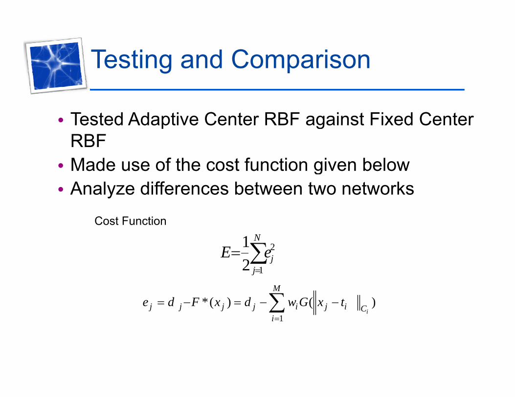
Testing and Comparisong

• Tested Adaptive Center RBF against Fixed CenterTested Adaptive Center RBF against Fixed Center RBF

• Made use of the cost function given belowg• Analyze differences between two networks

Cost Function

N

jjeE

1

2

21

Cost Function

j

1

*( ) ( )i

M

j j j j i j i Ci

e d F x d w G x t

Function Approximation

• "Plateau" function y = f(x1,x2) used in thisPlateau function y f(x1,x2) used in this example. The data are sampled in the domain -1<x1<1, -1<x2<1.

G. Bugmann, et all, "CLASSIFICATION USING NETWORKS OF NORMALIZED RADIAL BASIS FUNCTIONS", ICAPR 1998.

Function Approximation

• A) Function of a standard RBF net trained on 70 points sampled f “Pl t ” f ti P t 0 21 A RMSfrom “Plateau” function. Parameters: σ = 0.21, Average RMS error < 0.04 after 30 epochs. 50 hidden nodes

• B) Function of a standard RBF net with σ = 0.03. Figure produced f th f i di ti th iti f th 70 t i i d tfor the purpose of indicating the positions of the 70 training data.

Comparison of RBF and MLP• RBF has a single hidden layer, while MLP can have many

In MLP hidden and output neurons have the same• In MLP, hidden and output neurons have the same underlying function. In RBF, they are specialized into distinct functions

• In RBF, the output layer is linear, but in MLP, all neurons are nonlinear

• The hidden neurons in RBF calculate the Euclidean norm• The hidden neurons in RBF calculate the Euclidean norm of the input vector and the center, while in MLP the inner product of the input vector and the weight vector is

l l t dcalculated• MLPs construct global approximations to nonlinear input–

output mapping. RBF uses exponentially decaying p pp g p y y glocalized nonlinearities (e.g. Gaussians) to construct local approximations to nonlinear input–output mappings

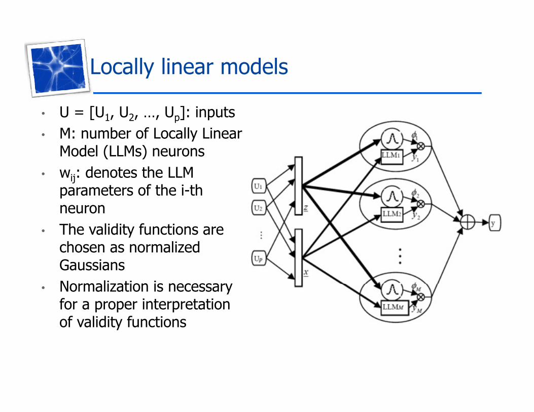
Locally linear modelsy

• U = [U1, U2, …, Up]: inputsM b f L ll Li• M: number of Locally Linear Model (LLMs) neurons

• wij: denotes the LLM ijparameters of the i-thneuron

• The validity functions areThe validity functions are chosen as normalized GaussiansNormalization is necessary• Normalization is necessary for a proper interpretation of validity functions

Locally linear modelsy

Locally Linear Model Tree (LoLiMoT) learning algorithm (Nelles 2001)learning algorithm (Nelles 2001)

1. Start with an initial model: Construct the validity functions for the initially given input space partitioning andfunctions for the initially given input space partitioning and estimate the LLM parameters. Set M to the initial number of LLMs. If no input space partitioning is available a priori, then

t M 1 d t t ith i l LLM hi h i f t i l b lset M=1 and start with a single LLM, which in fact is a global linear model since its validity function covers the whole input space with Φ1(x) = 1

Locally Linear Model Tree (LoLiMoT) learning algorithm (Nelles 2001)learning algorithm (Nelles 2001)

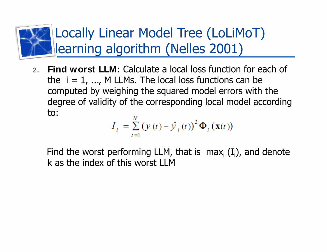
2. Find worst LLM: Calculate a local loss function for each of the i 1 M LLMs The local loss functions can bethe i = 1, ..., M LLMs. The local loss functions can be computed by weighing the squared model errors with the degree of validity of the corresponding local model according tto:

Find the worst performing LLM, that is maxi (Ii), and denote k as the index of this worst LLM

Locally Linear Model Tree (LoLiMoT) learning algorithm (Nelles 2001)learning algorithm (Nelles 2001)

3. Check all divisions: The k-th LLM is considered for further refinement The hyper rectangle of this LLM is split into tworefinement. The hyper-rectangle of this LLM is split into two halves with an axis-orthogonal split. Divisions in all dimensions are tried. For each division dim=1,…,P the f ll i t i d tfollowing steps are carried out: a. Construction of the multidimensional MFs for both hyper-

rectanglesb. Construction of all validity functionsc. Local estimation of the rule consequent parameters for

both newly generated LLMsboth newly generated LLMsd. Calculation of the loss function for the current overall

model

Locally Linear Model Tree (LoLiMoT) learning algorithm (Nelles 2001)learning algorithm (Nelles 2001)

Initial global linear modelInitial global linear model

Split along x1 or x2

Pick split that minimizesmodel error (residual)

Readingg

• S Haykin, Neural Networks: A Comprehensive y , pFoundation, 2007 (Chapter 6).