lectures 24 & 25 higher layer protocols: tcp/ip and atm · pdf filelectures 24 & 25...

Lectures 24 & 25

Higher Layer Protocols:TCP/IP and ATM

Eytan ModianoMassachusetts Institute of Technology

Laboratory for Information and Decision Systems

Eytan Modiano Slide 1

Outline

• Network Layer and Internetworking

• The TCP/IP protocol suit

• ATM

• MPLS


Higher Layers

Virtual link for reliable packets

Application

Presentation

Session

Transport

Network

Data link Control

Application

Presentation

Session

Transport

Network

Data link Control

Network Network

DLC DLC DLC DLC

Virtual bit pipe

Virtual link for end to end packets

Virtual link for end to end messages

Virtual session

Virtual network service

physical interfacephys. int. phys. int. phys. int. phys. int.

physical interface

TCP, UDP

IP, ATM

Physical link

External subnet subnet External Site node node site


Packet Switching

• Datagram packet switching – Route chosen on packet-by-packet basis – Different packets may follow different routes – Packets may arrive out of order at the destination – E.g., IP (The Internet Protocol)

• Virtual Circuit packet switching – All packets associated with a session follow the same path – Route is chosen at start of session – Packets are labeled with a VC# designating the route – The VC number must be unique on a given link but can change from

link to link Imagine having to set up connections between 1000 nodes in a mesh Unique VC numbers imply 1 Million VC numbers that must be representedand stored at each node

– E.g., ATM (Asynchronous transfer mode)


Virtual Circuits Packet Switching

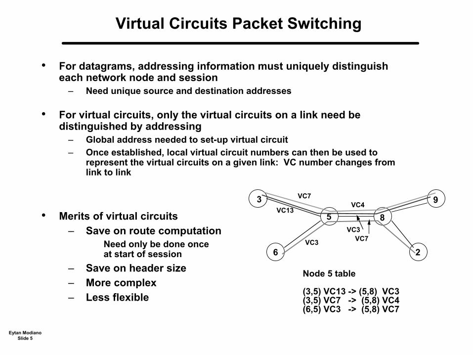
• For datagrams, addressing information must uniquely distinguisheach network node and session

– Need unique source and destination addresses

• For virtual circuits, only the virtual circuits on a link need be distinguished by addressing

– Global address needed to set-up virtual circuit – Once established, local virtual circuit numbers can then be used to

represent the virtual circuits on a given link: VC number changes fromlink to link

• Merits of virtual circuits – Save on route computation

Need only be done once at start of session

– Save on header size – More complex – Less flexible

3

6

5 8

2

9

VC3

VC13

VC7 VC4

VC3 VC7

Node 5 table

(3,5) VC13 -> (5,8) VC3 (3,5) VC7 -> (5,8) VC4(6,5) VC3 -> (5,8) VC7


The TCP/IP Protocol Suite

• Transmission Control Protocol / Internet Protocol

• Developed by DARPA to connect Universities and Research Labs

Four Layer model

Telnet, FTP, email, etc.

TCP, UDP

IP, ICMP, IGMP

�Device drivers, interface cards

TCP - Transmission Control ProtocolUDP - User Datagram ProtocolIP - Internet Protocol

Applications Transport Network

Link


Internetworking with TCP/IP

FTP FTP Protocol FTP client server

TCP Protocol TCPTCP

IP IP Protocol IP Protocol

Ethernet Ethernet Protocol

token driver

token ring Protocol

Ethernet

driver

IP ROUTER

IP

Ethernet driver

token driver

token

ring ring

ring


Encapsulation

14 20 20 4

Ethernet frame

46 to 1500 bytes

Ethernet

Ethernet

Application

user data

Appluser data header

TCPheader application

header IP TCP

header application

IP datagram

TCP header application header

IP Ethernet header

Ethernet trailer

driver

IP

TCP

TCP segment

data

data

data

Eytan ModianoSlide 8

Bridges, Routers and Gateways

• A Bridge is used to connect multiple LAN segments – Layer 2 routing (Ethernet) – Does not know IP address – Varying levels of sophistication

Simple bridges just forward packets smart bridges start looking like routers

• A Router is used to route connect between different networks using network layer address

– Within or between Autonomous Systems – Using same protocol (e.g., IP, ATM)

• A Gateway connects between networks using different protocols – Protocol conversion – Address resolution

• These definitions are often mixed and seem to evolve!


Bridges, routers and gateways

Ethernet A

Ethernet B Bridge

IP Router

Small company

Gateway Service provider’s

ATM backbone

ATM switches (routers)

Gateway

Another provider’s Frame Relay

Backbone


IP addresses

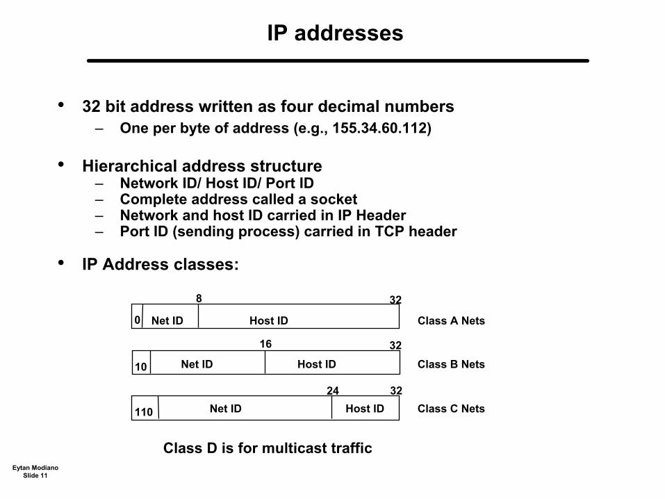
• 32 bit address written as four decimal numbers – One per byte of address (e.g., 155.34.60.112)

• Hierarchical address structure – Network ID/ Host ID/ Port ID – Complete address called a socket – Network and host ID carried in IP Header – Port ID (sending process) carried in TCP header

• IP Address classes:

8 32

Net ID Host ID

Net ID

Net ID

Host ID

Host ID

0

10

110

16 32

24 32

Class A Nets

Class B Nets

Class C Nets

Class D is for multicast trafficEytan Modiano

Slide 11

Host Names

• Each machine also has a unique name

• Domain name System: A distributed database that provides amapping between IP addresses and Host names

• E.g., 155.34.50.112 => plymouth.ll.mit.edu


Internet Standards

• Internet Engineering Task Force (IETF) – Development on near term internet standards – Open body – Meets 3 times a year

• Request for Comments (RFCs) – Official internet standards – Available from IETF web page: http://www.ietf.org


The Internet Protocol (IP)

• Routing of packet across the network • Unreliable service

– Best effort delivery – Recovery from lost packets must be done at higher layers

• Connectionless – Packets are delivered (routed) independently – Can be delivered out of order – Re-sequencing must be done at higher layers

• Current version V4

• Future V6 – Add more addresses (40 byte header!) – Ability to provide QoS


Header Fields in IP

1 4 8 16 32

Protocol

Note that the minimum size header is 20 bytes; TCP also has 20 byte header

Ver Header length type of service Total length (bytes)

16 - bit identification Flags 13 - bit fragment offset

TTL Header Checksum

Source IP Address

Destination IP Address

Options (if any)

Data


IP HEADER FIELDS

• Vers: Version # of IP (current version is 4) • HL: Header Length in 32-bit words • Service: Mostly Ignored • Total length Length of IP datagram • ID Unique datagram ID • Flags: NoFrag, More • FragOffset: Fragment offset in units of 8 Octets • TTL: Time to Live in "seconds” or Hops • Protocol: Higher Layer Protocol ID # • HDR Cksum: 16 bit 1's complement checksum (on header only!) • SA & DA: Network Addresses

• Options: Record Route,Source Route,TimeStamp


FRAGMENTATION

ethernet mtu=1500

X.25 G

GMTU = 512 ethernet mtu=1500

• A gateway fragments a datagram if length is too great for nextnetwork (fragmentation required because of unknown paths).

• Each fragment needs a unique identifier for datagram plusidentifier for position within datagram

• In IP, the datagram ID is a 16 bit field counting datagram fromgiven host


POSITION OF FRAGMENT

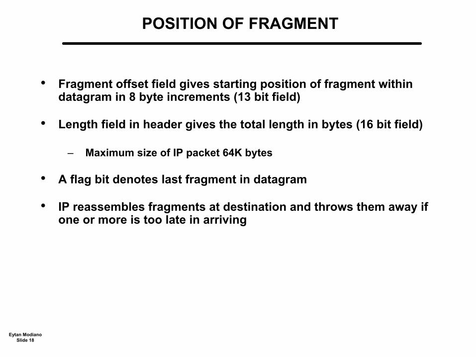
• Fragment offset field gives starting position of fragment withindatagram in 8 byte increments (13 bit field)

• Length field in header gives the total length in bytes (16 bit field)

– Maximum size of IP packet 64K bytes

• A flag bit denotes last fragment in datagram

• IP reassembles fragments at destination and throws them away ifone or more is too late in arriving


IP Routing

• Routing table at each node contains for each destination the nexthop router to which the packet should be sent

– Not all destination addresses are in the routing table Look for net ID of the destination “Prefix match” Use default router

• Routers do not compute the complete route to the destination butonly the next hop router

• IP uses distributed routing algorithms: RIP, OSPF • In a LAN, the “host” computer sends the packet to the default

router which provides a gateway to the outside world


Subnet addressing

• Class A and B addresses allocate too many hosts to a given net • Subnet addressing allows us to divide the host ID space into

smaller “sub networks” – Simplify routing within an organization – Smaller routing tables – Potentially allows the allocation of the same class B address to more

than one organization • 32 bit Subnet “Mask” is used to divide the host ID field into

subnets – “1” denotes a network address field – “0” denotes a host ID field

16 bit net ID 16 bit host ID Class B Address 140.252 Subnet ID Host ID

Mask 111111 111 1111111 11111111 00000000


Classless inter-domain routing (CIDR)

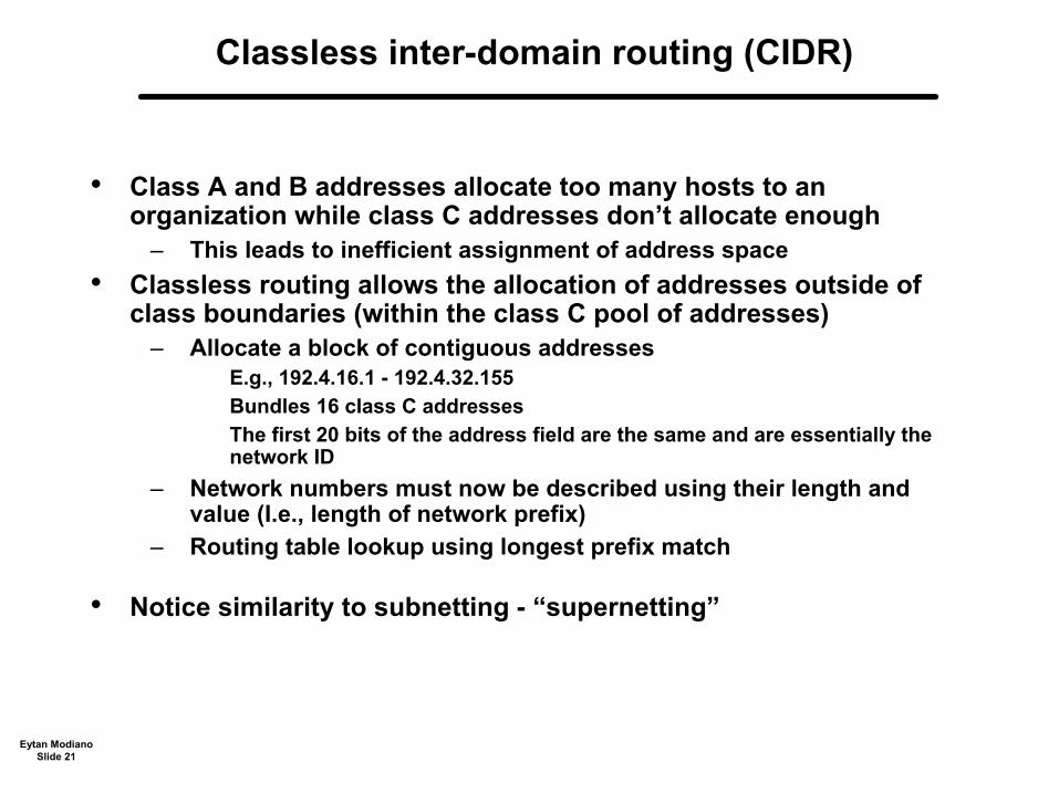
• Class A and B addresses allocate too many hosts to anorganization while class C addresses don’t allocate enough

– This leads to inefficient assignment of address space • Classless routing allows the allocation of addresses outside of

class boundaries (within the class C pool of addresses) – Allocate a block of contiguous addresses

E.g., 192.4.16.1 - 192.4.32.155 Bundles 16 class C addresses The first 20 bits of the address field are the same and are essentially the network ID

– Network numbers must now be described using their length andvalue (I.e., length of network prefix)

– Routing table lookup using longest prefix match

• Notice similarity to subnetting - “supernetting”


Dynamic Host Configuration (DHCP)

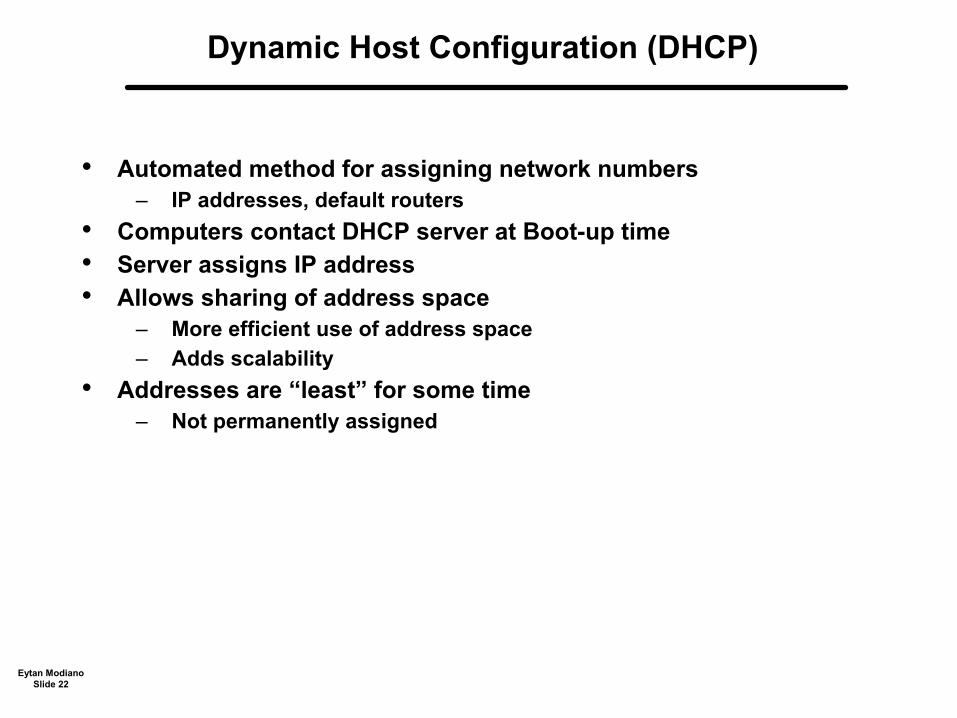
• Automated method for assigning network numbers – IP addresses, default routers

• Computers contact DHCP server at Boot-up time • Server assigns IP address • Allows sharing of address space

– More efficient use of address space – Adds scalability

• Addresses are “least” for some time – Not permanently assigned


Address Resolution Protocol

• IP addresses only make sense within IP suite • Local area networks, such as Ethernet, have their own addressing

scheme – To talk to a node on LAN one must have its physical address

(physical interface cards don’t recognize their IP addresses) • ARP provides a mapping between IP addresses and LAN

addresses • RARP provides mapping from LAN addresses to IP addresses • This is accomplished by sending a “broadcast” packet requesting

the owner of the IP address to respond with their physical address – All nodes on the LAN recognize the broadcast message – The owner of the IP address responds with its physical address

• An ARP cache is maintained at each node with recent mappings

ARP RARP IP

Ethernet


Routing in the Internet

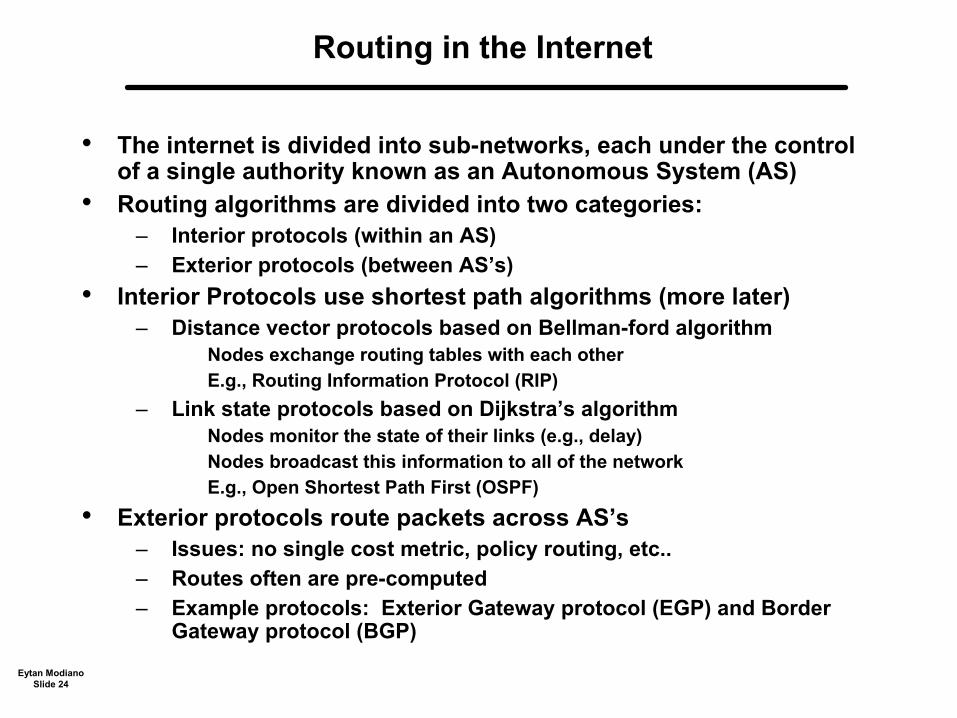
• The internet is divided into sub-networks, each under the control of a single authority known as an Autonomous System (AS)

• Routing algorithms are divided into two categories: – Interior protocols (within an AS) – Exterior protocols (between AS’s)

• Interior Protocols use shortest path algorithms (more later) – Distance vector protocols based on Bellman-ford algorithm

Nodes exchange routing tables with each other E.g., Routing Information Protocol (RIP)

– Link state protocols based on Dijkstra’s algorithm Nodes monitor the state of their links (e.g., delay) Nodes broadcast this information to all of the network E.g., Open Shortest Path First (OSPF)

• Exterior protocols route packets across AS’s – Issues: no single cost metric, policy routing, etc.. – Routes often are pre-computed – Example protocols: Exterior Gateway protocol (EGP) and Border

Gateway protocol (BGP) Eytan Modiano

Slide 24

IPv6

• Effort started in 1991 as IPng • Motivation

– Need to increase IP address space – Support for real time application - “QoS” – Security, Mobility, Auto-configuration

• Major changes – Increased address space (6 bytes)

1500 IP addresses per sq. ft. of earth! Address partition similar to CIDR

– Support for QoS via Flow Label field – Simplified header

• Most of the reasons for IPv6 have been taken care of in IPv4

– Is IPv6 really needed? – Complex transition from V4 to V6

0 ver class Flow label length Hop limitnexthd

Source address

Destination address


31

Resource Reservation (RSVP)

• Service classes (defined by IETF) – Best effort – Guaranteed service

Max packet delay – Controlled load

emulate lightly loaded network via priority queueing mechanism • Need to reserve resources at routers along the path • RSVP mechanism

– Packet classification Associate packets with sessions (use flow field in IPv6)

– Receiver initiated reservations to support multicast – “soft state” - temporary reservation that expires after 30 seconds

Simplify the management of connections Requires refresh messages

– Packet scheduling to guarantee service Proprietary mechanisms (e.g., Weighted fair queueing)

• Scalability Issues – Each router needs to keep track of large number of flows that grows

with the size (capacity) of the router Eytan Modiano

Slide 26

Differentiated Services (Diffserv)

• Unlike RSVP Diffserv does not need to keep track of individualflows

– Allocate resources to a small number of classes of traffic Queue packets of the same class together

– E.g., two classes of traffic - premium and regular Use one bit to differential between premium and regular packets

– Issues Who sets the premium bit? How is premium service different from regular?

• IETF propose to use TOS field in IP header to identifytraffic classes

– Potentially more than just two classes


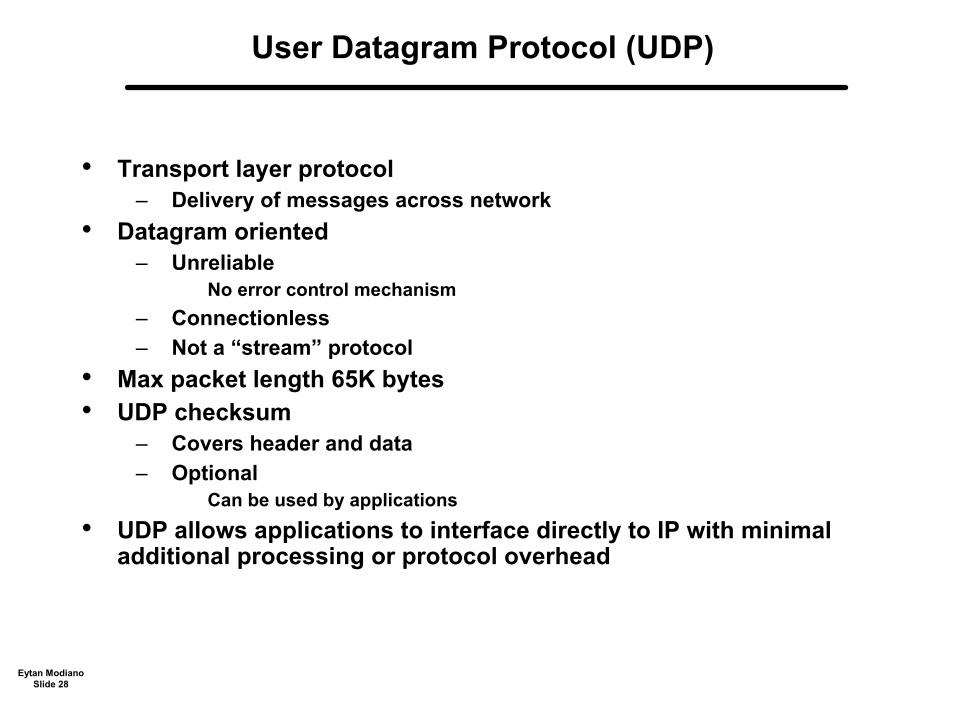
User Datagram Protocol (UDP)

• Transport layer protocol – Delivery of messages across network

• Datagram oriented – Unreliable

No error control mechanism – Connectionless – Not a “stream” protocol

• Max packet length 65K bytes • UDP checksum

– Covers header and data – Optional

Can be used by applications • UDP allows applications to interface directly to IP with minimal

additional processing or protocol overhead


UDP header format

IP Datagram

IP header UDP header data

16 bit source port number 16 bit destination port number 16 bit UDP length 16 bit checksum

Data

• The port numbers identifie the sending and receiving processes – I.e., FTP, email, etc.. – Allow UDP to multiplex the data onto a single stream

• UDP length = length of packet in bytes – Minimum of 8 and maximum of 2^16 - 1 = 65,535 bytes

• Checksum covers header and data – Optional, UDP does not do anything with the checksum


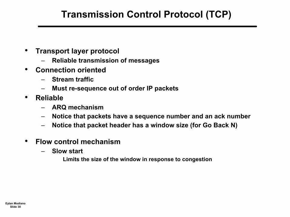
Transmission Control Protocol (TCP)

• Transport layer protocol – Reliable transmission of messages

• Connection oriented – Stream traffic – Must re-sequence out of order IP packets

• Reliable – ARQ mechanism – Notice that packets have a sequence number and an ack number – Notice that packet header has a window size (for Go Back N)

• Flow control mechanism – Slow start

Limits the size of the window in response to congestion


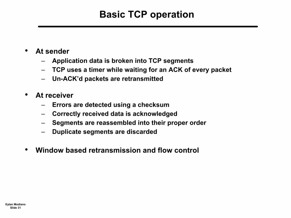
Basic TCP operation

• At sender – Application data is broken into TCP segments – TCP uses a timer while waiting for an ACK of every packet – Un-ACK’d packets are retransmitted

• At receiver – Errors are detected using a checksum – Correctly received data is acknowledged – Segments are reassembled into their proper order – Duplicate segments are discarded

• Window based retransmission and flow control


TCP header fields

16 32

Source port Destination port

Sequence number

Request number Data Offset Reserved Control Window

Check sum Urgent pointer

Options (if any)

Data


TCP header fields

• Ports number are the same as for UDP • 32 bit SN uniquely identify the application data contained in the

TCP segment – SN is in bytes! – It identify the first byte of data

• 32 bit RN is used for piggybacking ACK’s – RN indicates the next byte that the received is expecting – Implicit ACK for all of the bytes up to that point

• Data offset is a header length in 32 bit words (minimum 20 bytes) • Window size

– Used for error recovery (ARQ) and as a flow control mechanism Sender cannot have more than a window of packets in the networksimultaneously

– Specified in bytes Window scaling used to increase the window size in high speed networks

• Checksum covers the header and data


TCP error recovery

• Error recovery is done at multiple layers – Link, transport, application

• Transport layer error recovery is needed because – Packet losses can occur at network layer

E.g., buffer overflow – Some link layers may not be reliable

• SN and RN are used for error recovery in a similar way to Go BackN at the link layer

– Large SN needed for re-sequencing out of order packets • TCP uses a timeout mechanism for packet retransmission

– Timeout calculation – Fast retransmission


TCP timeout calculation

• Based on round trip time measurement (RTT) – Weighted average

RTT_AVE = a*(RTT_measured) + (1-a)*RTT_AVE

• Timeout is a multiple of RTT_AVE (usually two) – Short Timeout would lead to too many retransmissions – Long Timeout would lead to large delays and inefficiency

• In order to make Timeout be more tolerant of delay variations ithas been proposed (Jacobson) to set the timeout value based onthe standard deviation of RTT

Timeout = RTT_AVE + 4*RTT_SD

• In many TCP implementations the minimum value of Timeout is500 ms due to the clock granularity


Fast Retransmit

• When TCP receives a packet with a SN that is greater than theexpected SN, it sends an ACK packet with a request number of theexpected packet SN

– This could be due to out-of-order delivery or packet loss • If a packet is lost then duplicate RNs will be sent by TCP until the

packet it correctly received – But the packet will not be retransmitted until a Timeout occurs – This leads to added delay and inefficiency

• Fast retransmit assumes that if 3 duplicate RNs are received bythe sending module that the packet was lost

– After 3 duplicate RNs are received the packet is retransmitted – After retransmission, continue to send new data

• Fast retransmit allows TCP retransmission to behave more like Selective repeat ARQ

– Future option for selective ACKs (SACK)


TCP congestion control

• TCP uses its window size to perform end-to-end congestioncontrol

– More on window flow control later • Basic idea

– With window based ARQ the number of packets in the network cannot exceed the window size (CW)

Last_byte_sent (SN) - last_byte_ACK’d (RN) <= CW

• Transmission rate when using window flow control is equal to onewindow of packets every round trip time

R = CW/RTT

• By controlling the window size TCP effectively controls the rate


Effect Of Window Size

• The window size is the number of bytes that are allowed to be intransport simultaneously

WASTED BW

WINDOW WINDOW

• Too small a window prevents continuous transmission

• To allow continuous transmission window size must exceed round-tripdelay time


Length of a bit (traveling at 2/3C)

At 300 bps 1 bit = 415 miles 3000 miles = 7 bits

At 3.3 kbps 1 bit = 38 miles 3000 miles = 79 bits

At 56 kbps 1 bit = 2 miles 3000 miles = 1.5 kbits

At 1.5 Mbps 1 bit = 438 ft. 3000 miles = 36 kbits

At 150 Mbps 1 bit = 4.4 ft. 3000 miles = 3.6 Mbits

At 1 Gbps 1 bit = 8 inches 3000 miles = 240 Mbits


Dynamic adjustment of window size

• TCP starts with CW = 1 packet and increases the window sizeslowly as ACK’s are received

– Slow start phase – Congestion avoidance phase

• Slow start phase – During slow start TCP increases the window by one packet for every

ACK that is received – When CW = Threshold TCP goes to Congestion avoidance phase – Notice: during slow start CW doubles every round trip time

Exponential increase!

• Congestion avoidance phase – During congestion avoidance TCP increases the window by one

packet for every window of ACKs that it receives – Notice that during congestion avoidance CW increases by 1 every

round trip time - Linear increase!

• TCP continues to increase CW until congestion occurs


Reaction to congestion

• Many variations: Tahoe, Reno, Vegas • Basic idea: when congestion occurs decrease the window size • There are two congestion indication mechanisms

– Duplicate ACKs - could be due to temporary congestion – Timeout - more likely due to significant congstion

• TCP Reno - most common implementation

– If Timeout occurs, CW = 1 and go back to slow start phase

– If duplicate ACKs occur CW = CW/2 stay in congestion avoidancephase


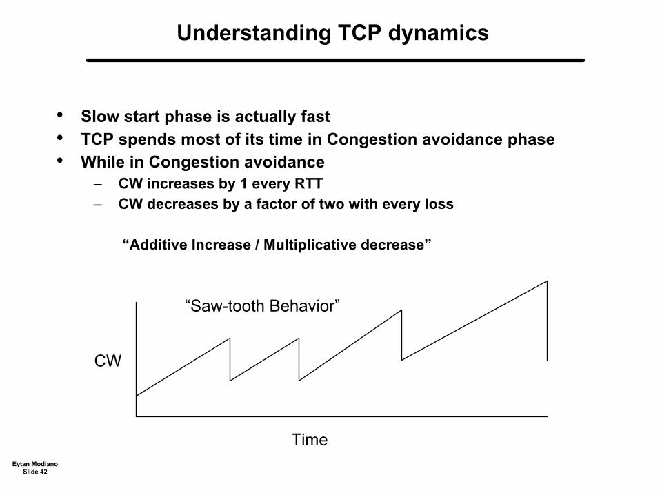
Understanding TCP dynamics

• Slow start phase is actually fast • TCP spends most of its time in Congestion avoidance phase • While in Congestion avoidance

– CW increases by 1 every RTT – CW decreases by a factor of two with every loss

“Additive Increase / Multiplicative decrease”

CW

“Saw-tooth Behavior”

TimeEytan Modiano

Slide 42

Random Early Detection (RED)

• Instead of dropping packet on queue overflow, drop them probabilistically earlier

• Motivation – Dropped packets are used as a mechanism to force the source to slow down

If we wait for buffer overflow it is in fact too late and we may have to drop many packets Leads to TCP synchronization problem where all sources slow down simultaneously

– RED provides an early indication of congestion Randomization reduces the TCP synchronization problem

• Mechanism – Use weighted average queue size

If AVE_Q > Tmin drop with prob. P If AVE_Q > Tmax drop with prob. 1

– RED can be used with explicit congestion notification rather than packet dropping

– RED has a fairness property Large flows more likely to be dropped

– Threshold and drop probability values are an area of active research

1

P max

Tmin Tmax

Ave queue length


TCP Error Control

EFFICIENCY VS. BER

CHANNEL BER

0

0.1

0.2

0.3

0.4

0.5

0.6

0.7

0.8

0.9

1

1E-07 1E-06 1E-05 1E-04 1E-03 1E-02

SRP 1 SEC R/T DELAY T-1 RATE 1000 BIT PACKETS

GO BACK N

WITH TCP WINDOW CONSTRAINT

• Original TCP designed for low BER, low delay links • Future versions (RFC 1323) will allow for larger windows and selective

retransmissions


Impact of transmission errors onTCP congestion control

EFFICIENCY VS BER FOR TCP'S CONGESTION CONTROL

BER

0 0.1 0.2 0.3 0.4 0.5 0.6 0.7 0.8 0.9

1

1.00E-07 1.00E-06 1.00E-05 1.00E-04 1.00E-03

1,544 KBPS 64 KBPS 16 KBPS

2.4 KBPS

• TCP assumes dropped packets are due to congestion and respondsby reducing the transmission rate

• Over a high BER link dropped packets are more likely to be due to errors than to congestion

• TCP extensions (RFC 1323) – Fast retransmit mechanism, fast recovery, window scaling


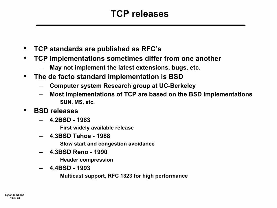
TCP releases

• TCP standards are published as RFC’s • TCP implementations sometimes differ from one another

– May not implement the latest extensions, bugs, etc. • The de facto standard implementation is BSD

– Computer system Research group at UC-Berkeley – Most implementations of TCP are based on the BSD implementations

SUN, MS, etc. • BSD releases

– 4.2BSD - 1983 First widely available release

– 4.3BSD Tahoe - 1988 Slow start and congestion avoidance

– 4.3BSD Reno - 1990 Header compression

– 4.4BSD - 1993 Multicast support, RFC 1323 for high performance


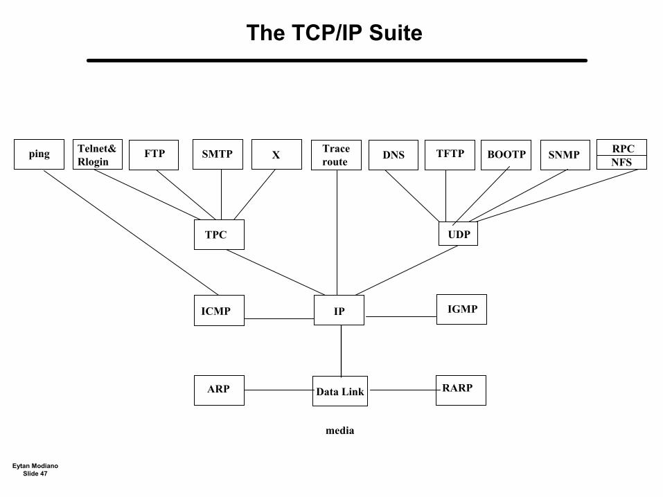
The TCP/IP Suite

UDP

Telnet& Rlogin

FTP SMTP X Trace route

ping DNS TFTP BOOTP SNMP NFS

TPC

ICMP

ARP

IP

Data Link RARP

IGMP

RPC

media


Asynchronous Transfer Mode (ATM)

• 1980’s effort by the phone companies to develop an integratednetwork standard (BISDN) that can support voice, data, video, etc.

• ATM uses small (53 Bytes) fixed size packets called “cells” – Why cells?

Cell switching has properties of both packet and circuit switching Easier to implement high speed switches

– Why 53 bytes? – Small cells are good for voice traffic (limit sampling delays)

For 64Kbps voice it takes 6 ms to fill a cell with data

• ATM networks are connection oriented – Virtual circuits


ATM Reference Architecture

• Upper layers – Applications – TCP/IP

• ATM adaptation layer – Similar to transport layer – Provides interface between

upper layers and ATM Break messages into cells and reassemble

• ATM layer – Cell switching – Congestion control

• Physical layer – ATM designed for SONET

Synchronous optical network TDMA transmission scheme with 125 µs frames

Upper Layers

AT M A daptation L ayer (A A L )

AT M

Physical


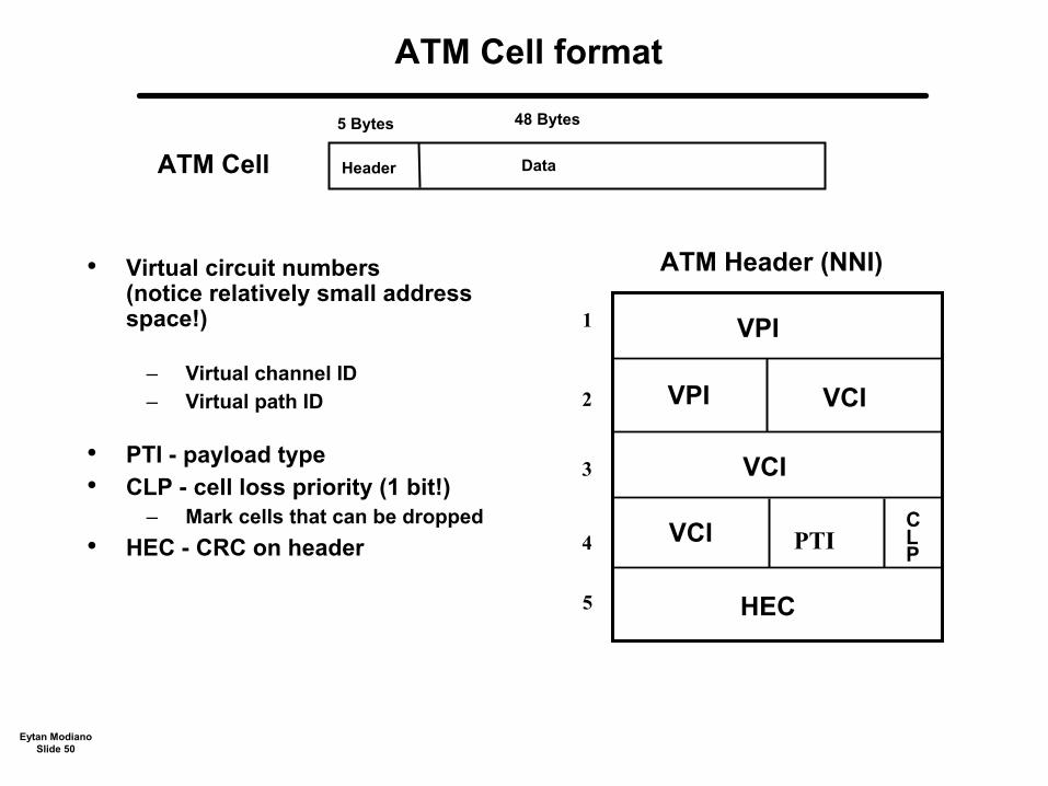
ATM Cell format

5 Bytes 48 Bytes

ATM Cell Header Data

• Virtual circuit numbers (notice relatively small addressspace!)

– Virtual channel ID – Virtual path ID

• PTI - payload type • CLP - cell loss priority (1 bit!)

– Mark cells that can be dropped • HEC - CRC on header

ATM Header (NNI)

1

2

3

4

5 HEC

PTI

VPI

C L P

VCI

VPI VCI

VCI


VPI/VCI

• VPI identifies a physical path between the source and destination • VCI identifies a logical connection (session) within that path

– Approach allows for smaller routing tablesand simplifies route computation

ATM Backbone

Use VPI for switching in backbone

Private network

Private network

Private network

Use VCI to ID connection Within private network


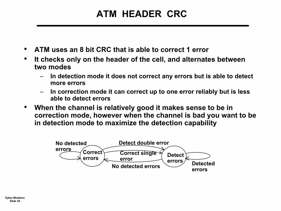
ATM HEADER CRC

• ATM uses an 8 bit CRC that is able to correct 1 error • It checks only on the header of the cell, and alternates between

two modes – In detection mode it does not correct any errors but is able to detect

more errors – In correction mode it can correct up to one error reliably but is less

able to detect errors • When the channel is relatively good it makes sense to be in

correction mode, however when the channel is bad you want to bein detection mode to maximize the detection capability

No detected Detect double error Correct errors Detect

errors

errors Correct single error

No detected errors Detected errors


ATM Service Categories

• Constant Bit Rate (CBR) - e.g. uncompressed voice – Circuit emulation

• Variable Bit Rate (rt-VBR) - e.g. compressed video – Real-time and non-real-time

• Available Bit Rate (ABR) - e.g. LAN interconnect – For bursty traffic with limited BW guarantees and congestion control

• Unspecified Bit Rate (UBR) - e.g. Internet – ABR without BW guarantees and congestion control


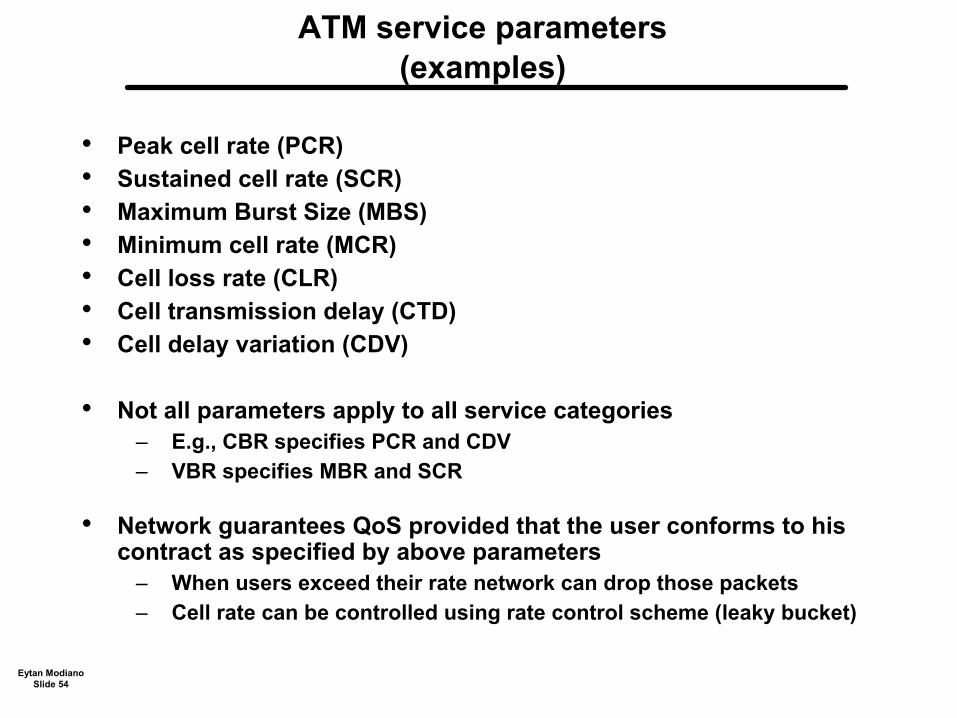
ATM service parameters(examples)

• Peak cell rate (PCR) • Sustained cell rate (SCR) • Maximum Burst Size (MBS) • Minimum cell rate (MCR) • Cell loss rate (CLR) • Cell transmission delay (CTD) • Cell delay variation (CDV)

• Not all parameters apply to all service categories – E.g., CBR specifies PCR and CDV – VBR specifies MBR and SCR

• Network guarantees QoS provided that the user conforms to his contract as specified by above parameters

– When users exceed their rate network can drop those packets – Cell rate can be controlled using rate control scheme (leaky bucket)


Flow control in ATM networks (ABR)

• ATM uses resource management cells to control rate parameters – Forward resource management (FRM) – Backward resource management (BRM)

• RM cells contain – Congestion indicator (CI) – No increase Indicator (NI) – Explicit cell rate (ER) – Current cell rate (CCR) – Min cell rate (MCR)

• Source generates RM cells regularly – As RM cells pass through the networked they can be marked with

CI=1 to indicate congestion – RM cells are returned back to the source where

CI = 1 => decrease rate by some fraction CI = 1 => Increase rate by some fraction

– ER can be used to set explicit rate


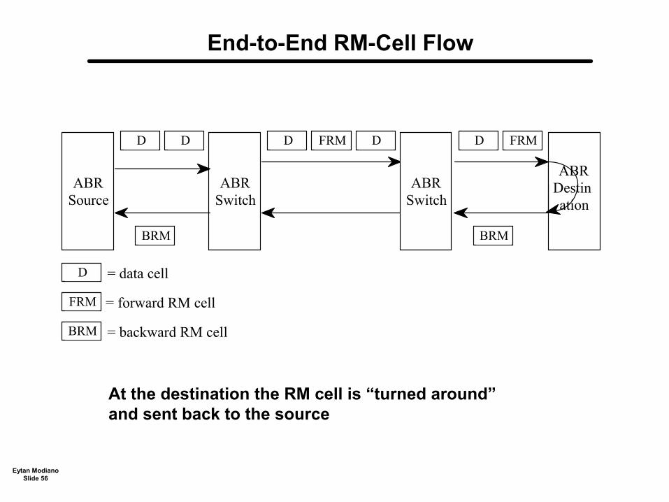
End-to-End RM-Cell Flow

ABR Switch

BRM

D D

ABR Switch

D FRM D

ABR Destination

BRM

D FRM

ABR Source

= data cell

= forward RM cell

= backward RM cell

At the destination the RM cell is “turned around” and sent back to the source

D

FRM

BRM


ATM Adaptation Layers

• Interface between ATM layer and higher layer packets • Four adaptation layers that closely correspond

to ATM’s service classes – AAL-1 to support CBR traffic – AAL-2 to support VBR traffic – AAL-3/4 to support bursty data traffic – AAL-5 to support IP with minimal overhead

• The functions and format of the adaptation layer depend on theclass of service.

– For example, stream type traffic requires sequence numbers to identify which cells have been dropped.

Each class of service has A different header format (in addition to the 5 byte ATM header)

USER PDU

ATM CELL

ATM CELL

(DLC or NL)


Example: AAL 3/4

ATM CELL PAYLOAD (48 Bytes)

ST SEQ MID LEN CRC

2 4 10 6 10 44 Byte User Payload

• ST: Segment Type (1st, Middle, Last) • SEQ:4-bit sequence number (detect lost cells) • MID: Message ID (reassembly of multiple msgs) • 44 Byte user payload (~84% efficient) • LEN: Length of data in this segment • CRC: 10 bit segment CRC

• AAL 3/4 allows multiplexing, reliability, & error detection but isfairly complex to process and adds much overhead

• AAL 5 was introduced to support IP traffic – Fewer functions but much less overhead and complexity


ATM cell switches

Input 1

Input Q's

Output Q's

S/W Control

Cell Processing

Cell Processing

Cell Processing

Switch Fabric

m

Output 1

Input 2 Output 2

Input Output m

• Design issues – Input vs. output queueing – Head of line blocking – Fabric speed


ATM summary

• ATM is mostly used as a “core” network technology

• ATM Advantages

– Ability to provide QoS – Ability to do traffic management – Fast cell switching using relatively short VC numbers

• ATM disadvantages – It not IP - most everything was design for TCP/IP – It’s not naturally an end-to-end protocol

Does not work well in heterogeneous environment Was not design to inter-operate with other protocols Not a good match for certain physical media (e.g., wireless)

– Many of the benefits of ATM can be “borrowed” by IP Cell switching core routers Label switching mechanisms


Multi-Protocol Label Switching (MPLS)

“As more services with fixed throughput anddelay requirements become more common, IP willneed virtual circuits (although it will probably callthem something else)”

RG, April 28, 1994


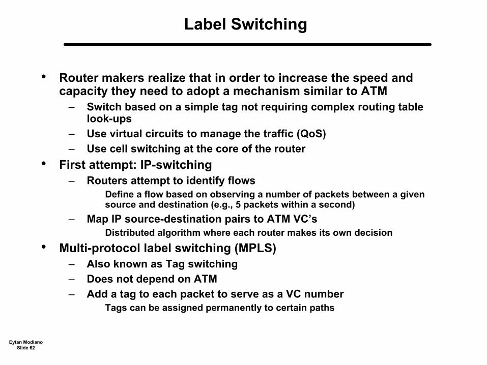
Label Switching

• Router makers realize that in order to increase the speed andcapacity they need to adopt a mechanism similar to ATM

– Switch based on a simple tag not requiring complex routing tablelook-ups

– Use virtual circuits to manage the traffic (QoS) – Use cell switching at the core of the router

• First attempt: IP-switching – Routers attempt to identify flows

Define a flow based on observing a number of packets between a givensource and destination (e.g., 5 packets within a second)

– Map IP source-destination pairs to ATM VC’s Distributed algorithm where each router makes its own decision

• Multi-protocol label switching (MPLS) – Also known as Tag switching – Does not depend on ATM – Add a tag to each packet to serve as a VC number

Tags can be assigned permanently to certain paths


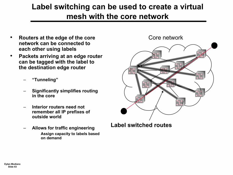
Label switching can be used to create a virtual mesh with the core network

• Routers at the edge of the corenetwork can be connected to each other using labels

• Packets arriving at an edge routercan be tagged with the label to the destination edge router

– “Tunneling”

– Significantly simplifies routingin the core

– Interior routers need not remember all IP prefixes of outside world

– Allows for traffic engineering Assign capacity to labels based on demand

Core network

Label switched routes

D

D


References

• TCP/IP Illustrated (Vols. 1&2), Stevens

• Computer Networks, Peterson and Davie

• High performance communication networks, Walrand and Varaiya



Class A

Class B

Class C

Class D

Class E

7 bits 24 bits

21 bits 8 bits

28 bits

netid hostid 011

netid hostid 01

netid hostid0111

27 bits

(reserved for future use)01111

netid hostid 0

14 bits 16 bits

lectures 24 & 25 higher layer protocols: tcp/ip and atm · pdf filelectures 24 & 25...

Documents