lectures 3 & 4: linear programming problem formulation

3/10/2010 Tibor Illés – Optimisation – 2009 1

Optimisation

Lectures 3 & 4:

Linear Programming Problem Formulation

Different forms of problems, elements of the simplex algorithm and sensitivity analysis

Lecturer: Tibor Illé[email protected]

mailto:[email protected]




Linear programming: problem description

A company produces four different (A, B, C, D) products from three different resources (R₁, R₂, R₃).

Resources Products CapacitiesA B C D

R₁ 1 0 2 1 280

R₂ 2 1 0 0 140

R₃ 0 1 1 1 120

Product prices 4 5 6 8

The resources are bounded by their capacities. The capacities of R₂ and R₃ should be used completely. From the products A and B in total we need to produces as much as from C.

From the product B we need to produce at least five unit more than from D.Maximize the profit !


Linear programming: problem formulation

Decision variables:x₁ is the # of picies produced

from product Ax₂ is the # of picies produced

from product Bx₃ is the # of picies produced

from product Cx₄ is the # of picies produced

from product D

Constraints:

Products

A B C D

R₁ 1 0 2 1 280

x₁ + 2 x₃ + x₄ ≤ 280

The capacities of R₂ and R₃ should be used completely.

R₂ 2 1 0 0 140

R₃ 0 1 1 1 120

2 x₁ + x₂ = 140x₂ + x₃ + x₄ = 120


Constraints:

Constraints and the objective function

From the products A and B in total we need to produces as much as from C.

x₁ + x₂ = x₃ orx₁ + x₂ - x₃ = 0

From the product B we need to produce at least five unit more than from D.

x₂ - x₄ ≥ 5

Objective function max 4 x₁ + 5 x₂ + 6 x₃ + 8 x₄


Linear programming problem

max 4 x₁ + 5 x₂ + 6 x₃ + 8 x₄Objective function

x₁ + 2 x₃ + x₄ ≤ 2802 x₁ + x₂ = 140

x₂ + x₃ + x₄ = 120x₁ + x₂ - x₃ = 0

x₂ - x₄ ≥ 5

Constraints

Sign constraints x₁, x₂, x₃, x₄ ≥ 0


Linear programming: problem description

In a factory using three machines (M₁, M₂, M₃) five different products (A₁, A₂, A₃, A₄, A₅) can be produced. All products are manufactured using all three machines. The processing time of different products are different on given machines. Specific processing times for different machines, theircapacities in working hours are shown on the following tables. The precies of different products are 2, 3, 2, 4, 2, respectively.

Machines Products CapacitiesA₁ A₂ A₃ A₄ A₅

M₁ 1 2 4 3 2 480

M₂ 3 1 1 5 3 460

M₃ 2 3 1 1 5 450

Maximize the profit under the following constraints:



a) The capacities of the machines can not be exceeded.b) From the product A₁ at least twice as much should be

produced as from A₅.c) Fr om the products A₂ and A₃ together can not be made

more than 120.

Decision variables: x₁, x₂, x₃, x₄, x₅ ≥ 0, are the decision variables [sign constraint on decision variables]

assigned to the products A₁, A₂, A₃, A₄, A₅, respectively.

Capacity constraints:[The information from the table and the verbal constraint a) is used.]

x₁ + 2x₂ + 4x₃ + 3x₄ + 2x₅ ≤ 4803x₁ + x₂ + x₃ + 5x₄ + 3x₅ ≤ 4602x₁ + 3x₂ + x₃ + x₄ + 5x₅ ≤ 450



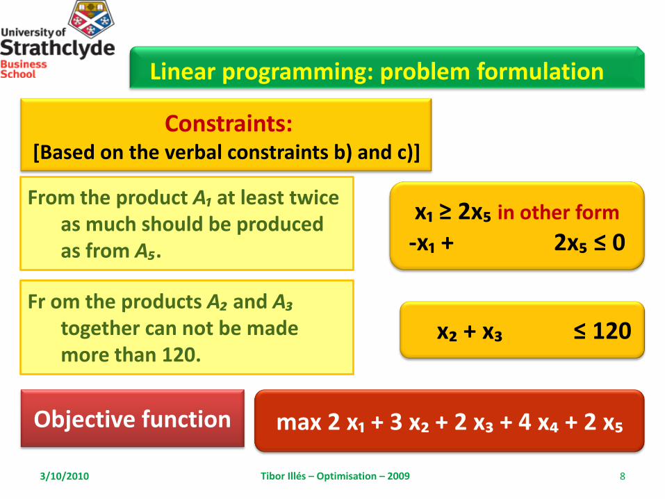
Constraints:[Based on the verbal constraints b) and c)]

x₂ + x₃ ≤ 120

From the product A₁ at least twice as much should be produced as from A₅.

Fr om the products A₂ and A₃together can not be made more than 120.

x₁ ≥ 2x₅ in other form

-x₁ + 2x₅ ≤ 0

Objective function max 2 x₁ + 3 x₂ + 2 x₃ + 4 x₄ + 2 x₅


Linear programming problem


-x₁ + 2x₅ ≤ 0x₂ + x₃ ≤ 120

Constraints

Sign constraints x₁, x₂, x₃, x₄, x₅ ≥ 0

Objective function max 2 x₁ + 3 x₂ + 2 x₃ + 4 x₄ + 2 x₅

Standardlinear

programmingproblem


Transportation problem/linear programming problem

min 18 x11 + 12 x12 + 13 x13 + 14 x14 + 9 x21 + 12 x22 + 11 x23 + 15 x24 + 9 x31 + 12 x32 + 17 x33 + 20 x34

x11 + x12 + x13 + x14 = 370

x21 + x22 + x23 + x24 = 620

x31 + x32 + x33 + x34 = 440

x11 + x21 + x31 = 220

x12 + x22 + x32 = 380

x13 + x23 + x33 = 410

x14 + x24 + x34 = 420

x11, x12, x13, x14, x21, x22, x23, x24, x31, x32, x33, x34 ≥ 0

Objective function

Constraints

Sign constraints


Transportation problem/linear programming problem

min 18 x11 + 12 x12 + 13 x13 + 14 x14 + 9 x21 + 12 x22 + 11 x23 + 15 x24 + 9 x31 + 12 x32 + 17 x33 + 20 x34

x11 + x12 + x13 + x14 = 370

x21 + x22 + x23 + x24 = 620

x31 + x32 + x33 + x34 = 440

x11 + x21 + x31 = 220

x12 + x22 + x32 = 380

x13 + x23 + x33 = 410

x14 + x24 + x34 = 420

x11, x12, x13, x14, x21, x22, x23, x24, x31, x32, x33, x34 ≥ 0

Objective functionConstraints

Sign constraints

Priority routes:Case 3 – upper

boundsx₁₂ ≤ 110x₃₃ ≤ 180

120 ≤ x₂₄ ≤ 320


Transportation problem: mathematical formulation

Linear programming formulation:

min c xA x = b

x ≥ 0

Simplex tableau


Standard linear programming problem


-x₁ + 2x₅ ≤ 0x₂ + x₃ ≤ 120

x₁, x₂, x₃, x₄, x₅ ≥ 0

max 2 x₁ + 3 x₂ + 2 x₃ + 4 x₄ + 2 x₅ 2x₁ + 3x₂ + 2x₃ + 4x₄ + 2x₅ - z = 0x₁ + 2x₂ + 4x₃ + 3x₄ + 2x₅ + s₁ = 480

3x₁ + x₂ + x₃ + 5x₄ + 3x₅ + s₂ = 4602x₁ + 3x₂ + x₃ + x₄ + 5x₅ + s₃ = 450-x₁ + 2x₅ + s₄ = 0

x₂ + x₃ + s₅ = 120x₁, x₂, x₃, x₄, x₅, s₁, s₂, s₃, s₄, s₅ ≥ 0

max z

x₁ x₂ x₃ x₄ x₅ s₁ s₂ s₃ s₄ s₅ z b

s₁ 1 2 4 3 2 1 0 0 0 0 0 480

s₂ 3 1 1 5 3 0 1 0 0 0 0 460

s₃ 2 3 1 1 5 0 0 1 0 0 0 450

s₄ -1 0 0 0 2 0 0 0 1 0 0 0

s₅ 0 1 1 0 0 0 0 0 0 1 0 120

z 2 3 2 4 2 0 0 0 0 0 -1 0

x₁ x₂ x₃ x₄ x₅ b

s₁ 1 2 4 3 2 480

s₂ 3 1 1 5 3 460

s₃ 2 3 1 1 5 450

s₄ -1 0 0 0 2 0

s₅ 0 1 1 0 0 120

z 2 3 2 4 2 0


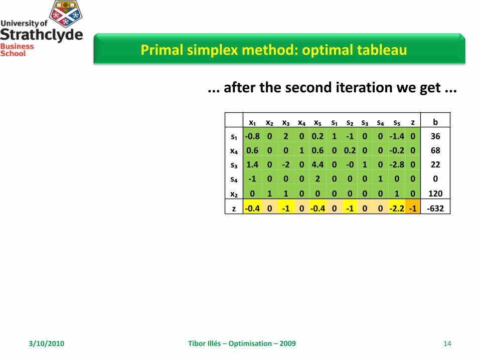
Primal simplex method: optimal tableau

... after the second iteration we get ...

x₁ x₂ x₃ x₄ x₅ s₁ s₂ s₃ s₄ s₅ z b

s₁ -0.8 0 2 0 0.2 1 -1 0 0 -1.4 0 36

x₄ 0.6 0 0 1 0.6 0 0.2 0 0 -0.2 0 68

s₃ 1.4 0 -2 0 4.4 0 -0 1 0 -2.8 0 22

s₄ -1 0 0 0 2 0 0 0 1 0 0 0

x₂ 0 1 1 0 0 0 0 0 0 1 0 120

z -0.4 0 -1 0 -0.4 0 -1 0 0 -2.2 -1 -632


Objective function coefficients

The matrix of the problem

Linear programming problem: Excel solver

Variables

Initial valuesx₁ x₂ x₃ x₄ x₅

0 0 0 0 0

1 2 4 3 2 0 4803 1 1 5 3 0 4602 3 1 1 5 0 450

-1 0 0 0 2 0 00 1 1 0 0 0 120

2 3 2 4 2 0

Righthand sidevalues

Constraint formulation

Relations between lefthand side and

righthand side values



OptionsLinear constraints

Sign constraints on variables


Excel solver: answer report

Microsoft Excel 12.0 Answer Report

Worksheet: [tutorial-examples.xlsx]Sheet2

Report Created: 30/10/2007 22:30:52

Target Cell (Max)

Cell Name Original Value Final Value

$K$14 objfun 632 632

Adjustable Cells


$E$6 x₁ 0 0

$F$6 x₂ 120 120

$G$6 x₃ 0 0

$H$6 x₄ 68 68

$I$6 x₅ 0 0

Constraints

Cell Name Cell Value Formula Status Slack

$K$8 const1 444 $K$8<=$L$8 Not Binding 36

$K$9 const2 460 $K$9<=$L$9 Binding 0





x₁ x₂ x₃ x₄ x₅ s₁ s₂ s₃ s₄ s₅ z b

s₁ -0.8 0 2 0 0.2 1 -1 0 0 -1.4 0 36

x₄ 0.6 0 0 1 0.6 0 0.2 0 0 -0.2 0 68

s₃ 1.4 0 -2 0 4.4 0 -0 1 0 -2.8 0 22

s₄ -1 0 0 0 2 0 0 0 1 0 0 0

x₂ 0 1 1 0 0 0 0 0 0 1 0 120

z -0.4 0 -1 0 -0.4 0 -1 0 0 -2.2 -1 -632


Primal simplex method: optimal tableau


x₁ x₂ x₃ x₄ x₅ s₁ s₂ s₃ s₄ s₅ z b

s₁ -0.8 0 2 0 0.2 1 -1 0 0 -1.4 0 36

x₄ 0.6 0 0 1 0.6 0 0.2 0 0 -0.2 0 68

s₃ 1.4 0 -2 0 4.4 0 -0 1 0 -2.8 0 22

s₄ -1 0 0 0 2 0 0 0 1 0 0 0

x₂ 0 1 1 0 0 0 0 0 0 1 0 120

z -0.4 0 -1 0 -0.4 0 -1 0 0 -2.2 -1 -632

Negative reduced cost have 5 variables: x₁, x₃, x₅, s₂ & s₅.s₅ has reduced cost -2.2 and since s₅ = 0, the resource 5 has been fully used.If we force s₅ to enter the basis then the objective function value will decrease (bad pivot column). Any unused unit of resource 5 will decrease the OF by 2.2.

Opportunity cost: the increase in the value of the OF that would occur if we could obtain an extra unit of this scare resource over and above the current supply limit




$K$14 objfun 632 632

Cell Name Original Value Final Value$E$6 x₁ 0 0$F$6 x₂ 120 120

$G$6 x₃ 0 0$H$6 x₄ 68 68

$I$6 x₅ 0 0

Target Cell (Max)


$K$14 objfun 634.2 634.2

Adjustable Cells


$E$6 x₁ 0 0

$F$6 x₂ 121 121

$G$6 x₃ 0 0

$H$6 x₄ 67.8 67.8

$I$6 x₅ 0 0

Constraints


$K$8 const1 445.4 $K$8<=$L$8 Not Binding 34.6




$K$12 const5 121 $K$12<=$L$12 Binding 0 Why ?


Opportunity cost: how much more of this resource to use?

x₁ x₂ x₃ x₄ x₅ s₁ s₂ s₃ s₄ s₅ z b

s₁ -0.8 0 2 0 0.2 1 -1 0 0 -1.4 0 36

x₄ 0.6 0 0 1 0.6 0 0.2 0 0 -0.2 0 68

s₃ 1.4 0 -2 0 4.4 0 -0 1 0 -2.8 0 22

s₄ -1 0 0 0 2 0 0 0 1 0 0 0

x₂ 0 1 1 0 0 0 0 0 0 1 0 120

z -0.4 0 -1 0 -0.4 0 -1 0 0 -2.2 -1 -632

Increasing by 1 unit the 5th resource, it will force the following changes:s₁ = 36 – 1.4 = 34.6x₄ = 68 – 0.2 = 67.8s₃ = 22 – 2.8 = 19.2s₄ = 0 + 0 = 0x₂ = 120 + 1 = 121OF = 632 + 2.2 = 634.2

Fully coincides with the Excel solution!

max 2 x₁ + 3 x₂ + 2 x₃ + 4 x₄ + 2 x₅

4*(-0.2) + 3 *1 = 2.2

min {36/1.4, 68/0.2, 22/2.8} = = min { 25.71, 340, 7.86} = 7.86


Changing resource 5 to 127 and 128

For computation use Excel solver and readWisniewski & Dacre: Optimization models for business and management decision making,

McGraw-Hill Book Co., 1990, chapter 8 on sensitivity analysis

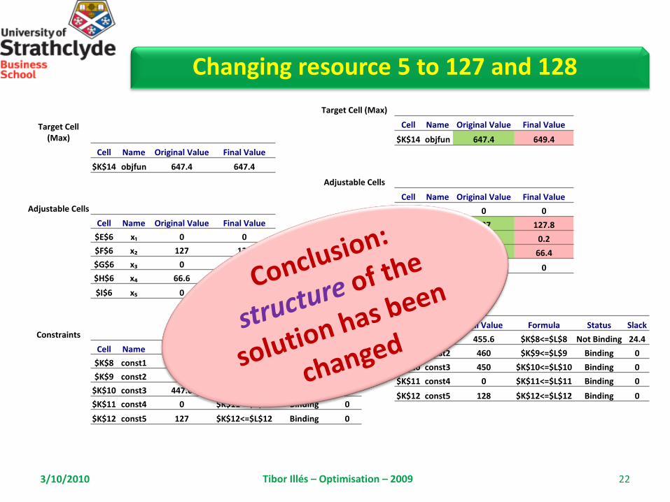
Target Cell (Max)


$K$14 objfun 647.4 649.4

Adjustable Cells


$E$6 x₁ 0 0

$F$6 x₂ 127 127.8

$G$6 x₃ 0 0.2

$H$6 x₄ 66.6 66.4

$I$6 x₅ 0 0

Constraints








Target Cell (Max)


$K$14 objfun 647.4 647.4

Adjustable Cells


$E$6 x₁ 0 0

$F$6 x₂ 127 127

$G$6 x₃ 0 0

$H$6 x₄ 66.6 66.6

$I$6 x₅ 0 0

Constraints







Changing resource 5 to 127 and 128


Excel solver: sensitivity report

Microsoft Excel 12.0 Sensitivity Report

Worksheet: [tutorial-examples.xlsx]Sheet2

Report Created: 30/10/2007 22:30:52

Adjustable Cells

Final Reduced Objective Allowable Allowable

Cell Name Value Cost Coefficient Increase Decrease

$E$6 x₁ 0 -0.4 2 0.400000004 1E+30

$F$6 x₂ 120 0 3 1E+30 1

$G$6 x₃ 0 -1 2 1 1E+30

$H$6 x₄ 68 0 4 11 0.66667

$I$6 x₅ 0 -0.4 2 0.400000004 1E+30

Constraints

Final Shadow Constraint Allowable Allowable

Cell Name Value Price R.H. Side Increase Decrease

$K$8 const1 444 0 480 1E+30 36

$K$9 const2 460 0.8 460 60 340

$K$10 const3 428 0 450 1E+30 22

$K$11 const4 0 0 0 1E+30 0

$K$12 const5 120 2.2 120 7.857142857 120

444 ≤ b₁ 120 ≤ b₂ ≤ 520428 ≤ b₃

0 ≤ b₄0 ≤ b₅ < 127.86

c₁ < 2.40012 ≤ c₂

c₃ ≤ 33.33 < c₄ ≤ 15

c₅ < 2.4001

then the basis is unchanged, thus only x₂ and x₄ are in the basis.

If the values of ci and bj are changing in thegiven intervals


Excel solver: sensitivity analysis – test problem

x₁ x₂ x₃ x₄ x₅

0 100 0 20 0

const1 1 2 4 3 2 260 500

const2 3 1 1 5 3 200 200

const3 2 3 1 1 5 320 500

const4 -1 0 0 0 2 0 100

const5 0 1 1 0 0 100 100

objfun 1 4 1 6 1 520

c₁ < 2.40012 ≤ c₂

c₃ ≤ 33.33 < c₄ ≤ 15

c₅ < 2.4001

Same solution structure.

Target Cell (Max)


$K$14 objfun 520 520

Adjustable Cells


$E$6 x₁ 0 0

$F$6 x₂ 100 100

$G$6 x₃ 0 0

$H$6 x₄ 20 20

$I$6 x₅ 0 0

Constraints







444 ≤ b₁ 120 ≤ b₂ ≤ 520428 ≤ b₃

0 ≤ b₄0 ≤ b₅ < 127.86



Microsoft Excel 12.0 Limits Report

Worksheet: [tutorial-examples.xlsx]Limits Report 1

Report Created: 30/10/2007 22:30:53

TargetCell Name Value

$K$14 objfun 632

Adjustable Lower Target Upper TargetCell Name Value Limit Result Limit Result

$E$6 x₁ 0 0 632 1.9E-14 632$F$6 x₂ 120 0 272 120 632$G$6 x₃ 0 0 632 0 632$H$6 x₄ 68 0 360 68 632$I$6 x₅ 0 0 632 0 632


(Primal) simplex algorithm: standard problem

Input: standard LP probleminitial basic feasible

solution is given

Is current solution optimal ?

(optimality criterion)

Find pivot column (positive reduced cost value).

Iscurrent solution

unbounded ?(unboundedness criterion)

Apply the ratio test, determine the pivot position, compute the

new solution.

StopOptimal solution

no

yes

yes

StopUnbounded LP

no


General LP problem and simplex algorithm: summary

Linear programming problem:• standard form (maximization problem, less-than-equal type constraints, sign restricted

variables, non-negative right hand side vector)• initial feasible basis (initial basic tableau, basic & non-basic variables, basic feasible

solution)• slack and artificial variables (transforming general LP problems using slack and

artificial variables into the 1st phase problem that has initial feasible basis)• sensitivity analysis of linear programming problems

Simplex algorithm (Dantzig, 1947):• elementary row operations • pivoting (pivot row and pivot column, [bad and good] pivot position)• optimality and unboundedness criteria• solving standard linear programming problems using simplex algorithm• solving general linear programming problems (two phase simplex algorithm)• Excel LP solver

3/10/2010 Tibor Illés – Optimisation - 2008 29

Standard linear programming problem


-x₁ + 2x₅ ≤ 0x₂ + x₃ ≤ 120

x₁, x₂, x₃, x₄, x₅ ≥ 0

max 2 x₁ + 3 x₂ + 2 x₃ + 4 x₄ + 2 x₅ 2x₁ + 3x₂ + 2x₃ + 4x₄ + 2x₅ - z = 0x₁ + 2x₂ + 4x₃ + 3x₄ + 2x₅ + s₁ = 480

3x₁ + x₂ + x₃ + 5x₄ + 3x₅ + s₂ = 4602x₁ + 3x₂ + x₃ + x₄ + 5x₅ + s₃ = 450-x₁ + 2x₅ + s₄ = 0

x₂ + x₃ + s₅ = 120x₁, x₂, x₃, x₄, x₅, s₁, s₂, s₃, s₄, s₅ ≥ 0

max z

x₁ x₂ x₃ x₄ x₅ s₁ s₂ s₃ s₄ s₅ z b

s₁ 1 2 4 3 2 1 0 0 0 0 0 480

s₂ 3 1 1 5 3 0 1 0 0 0 0 460

s₃ 2 3 1 1 5 0 0 1 0 0 0 450

s₄ -1 0 0 0 2 0 0 0 1 0 0 0

s₅ 0 1 1 0 0 0 0 0 0 1 0 120

z 2 3 2 4 2 0 0 0 0 0 -1 0

x₁ x₂ x₃ x₄ x₅ b

s₁ 1 2 4 3 2 480

s₂ 3 1 1 5 3 460

s₃ 2 3 1 1 5 450

s₄ -1 0 0 0 2 0

s₅ 0 1 1 0 0 120

z 2 3 2 4 2 0


LP problem: general form

max 4 x₁ + 5 x₂ + 6 x₃ + 8 x₄

x₁ + 2 x₃ + x₄ ≤ 280

2 x₁ + x₂ = 140x₂ + x₃ + x₄ = 120

x₁ + x₂ - x₃ = 0x₂ - x₄ ≥ 5

x₁, x₂, x₃, x₄ ≥ 0

max z

4 x₁ + 5 x₂ + 6 x₃ + 8 x₄ - z =0x₁ + 2 x₃ + x₄ + s₁ =280

2 x₁ + x₂ + w₂ = 140x₂ + x₃ + x₄ + w₃ = 120

x₁ + x₂ - x₃ + w₄ = 0x₂ - x₄ - s₅ + w₅ = 5

x₁, x₂, x₃, x₄, x₅, s₁, s₅, w₂, w₃, w₄, w₅ ≥ 0

min w₂ + w₃ + w₄ + w₅

1st phase problem

2nd phase problem

max - w₂ - w₃ - w₄ - w₅

Decision variables: x₁, x₂, x₃, x₄, x₅

Slack variables: s₁, s₅

Artificial variables: w₂, w₃, w₄, w₅


General LP problem: bounded variables

max -3 x₁ - x₂ - x₃ + 2 x₄ - x₅ + x₆ + x₇ - 4 x₈

x₁ + 3 x₃ + x₄ - 5 x₅ - 2 x₆ + 4 x₇ - 6 x₈ = 7x₂ - 2 x₃ - x₄ + 4 x₅ + x₆ - 3 x₇ + 5 x₈ = -3

0 ≤ x₁ ≤ 8, 0 ≤ x₂ ≤ 6, 0 ≤ x₃ ≤ 4, 0 ≤ x₄ ≤ 150 ≤ x₅ ≤ 2, 0 ≤ x₆ ≤ 10, 0 ≤ x₇ ≤ 10, 0 ≤ x₈ ≤ 3

Simplex algorithm can be modified to deal with bounded variables. For the Excel solver you should enter these bounds as constraints and simply solve the problem.


x₁ x₂ x₃ x₄ x₅ x₆ x₇ x₈

0 0 0 0 0 0 0 0

constraint1 1 0 3 1 -5 -2 4 -6 0 7constraint2 0 1 -2 -1 4 1 -3 5 0 -3

bound1 1 0 0 0 0 0 0 0 0 8bound2 0 1 0 0 0 0 0 0 0 6

bound3 0 0 1 0 0 0 0 0 0 4bound4 0 0 0 1 0 0 0 0 0 15

bound5 0 0 0 0 1 0 0 0 0 2

bound6 0 0 0 0 0 1 0 0 0 10bound7 0 0 0 0 0 0 1 0 0 10

bound8 0 0 0 0 0 0 0 1 0 3

obj fun -3 -1 -1 2 -1 1 1 -4 0

General LP problem: Excel solver data

Why ?


General LP problem: How to use Excel solver ?

x₁ x₂ x₃ x₄ x₅ x₆ x₇ x₈

0 6 0 15 2 1 1 0

constraint1 1 0 3 1 -5 -2 4 -6 7 7

constraint2 0 1 -2 -1 4 1 -3 5 -3 -3

bound1 1 0 0 0 0 0 0 0 0 8

bound2 0 1 0 0 0 0 0 0 6 6

bound3 0 0 1 0 0 0 0 0 0 4

bound4 0 0 0 1 0 0 0 0 15 15

bound5 0 0 0 0 1 0 0 0 2 2

bound6 0 0 0 0 0 1 0 0 1 10

obj fun -3 -1 -1 2 -1 1 1 -4 24

Constraints


$L$6 constraint1 7 $L$6=$M$6 Not Binding 0

$L$7 constraint2 -3 $L$7=$M$7 Not Binding 0

$L$8 bound1 0 $L$8<=$M$8 Not Binding 8

$L$9 bound2 6 $L$9<=$M$9 Binding 0





Adjustable Cells



$C$4 x₁ 0 -1 -3 1 1E+30

$D$4 x₂ 6 0 -1 1E+30 2

$E$4 x₃ 0 -1 -1 1 1E+30

$F$4 x₄ 15 0 2 1E+30 1

$G$4 x₅ 2 0 -1 1E+30 1

$H$4 x₆ 1 0 1 0.666666667 1

$I$4 x₇ 1 0 1 0.5 0.666666667

$J$4 x₈ 0 -1 -4 1 1E+30

Optimal solution !

Even if we add the bound on x₇ the same solution remains

feasible and optimal, too. Thus the bound on x₈ made the

problem infeasible.


General LP problem: unbounded or free variables

max x₁ + x₇

x₁ + x₂ + x₃ + x₄ + x₅ + x₆ - x₇ = 10x₁ + 2x₂ + x₇ = 2

x₃ + 2x₄ + x₇ = 5x₅ + 2x₆ + x₇ = 8

x₁, x₂, x₃, x₄, x₅, x₆ ≥ 0 and x₇ is an unbounded (free) variable

Express x₇ from any of the given equations and substitute backinto other equations and into the objective function as well.

x₇ = 8 - x₅ - 2x₆


max x₁ - x₅ - 2x₆ + 8

General LP problem: unbounded or free variables

x₁ + x₂ + x₃ + x₄ + 2x₅ + 3x₆ = 18x₁ + 2x₂ - x₅ - 2x₆ = -6

x₃ + 2x₄ - x₅ - 2x₆ = -3

x₁, x₂, x₃, x₄, x₅, x₆ ≥ 0

x₁ + x₂ + x₃ + x₄ + 2x₅ + 3x₆ = 18- x₁ - 2x₂ + x₅ + 2x₆ = 6

- x₃ - 2x₄ + x₅ + 2x₆ = 3

# of variables and constrains are reduced.

Multiply the 2nd and the 3rd equations by -1


Solving general LP problem by simplex algorithm

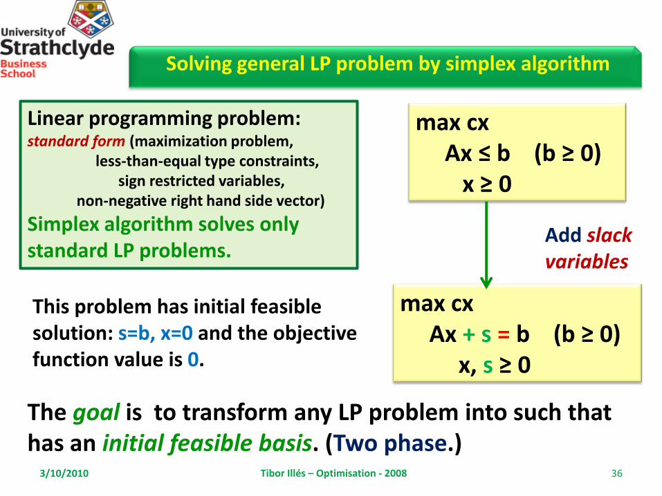
Linear programming problem:standard form (maximization problem,

less-than-equal type constraints, sign restricted variables,

non-negative right hand side vector)

Simplex algorithm solves only standard LP problems.

max cxAx ≤ b (b ≥ 0)

x ≥ 0

Add slack variables

max cxAx + s = b (b ≥ 0)

x, s ≥ 0

This problem has initial feasible solution: s=b, x=0 and the objective function value is 0.

The goal is to transform any LP problem into such that has an initial feasible basis. (Two phase.)


Solving general LP problem by simplex algorithm

General LP problem.• Using slack variables transform the constraints into equations.• If we have bounded or unbounded variables then (i)

eliminate unbounded variables [in this way the number of variables and equations will be reduced], (ii) transform the bounded variables into such new variables that has 0 as lower bound.

• Multiply any equation by -1 if it is necessary to get non-negative right hand side.• If the transformed problem has initial feasible basis then we can solve it by using the simplex algorithm [or modified SA that handles bounded variables], otherwise we should introduce artificial variables to obtain the first phase LP problem.

General LP problems for the state-of-the-art

linear programming solvers(CPLEX, XPRESS-MP, Excel)

without any transformation can be fed.


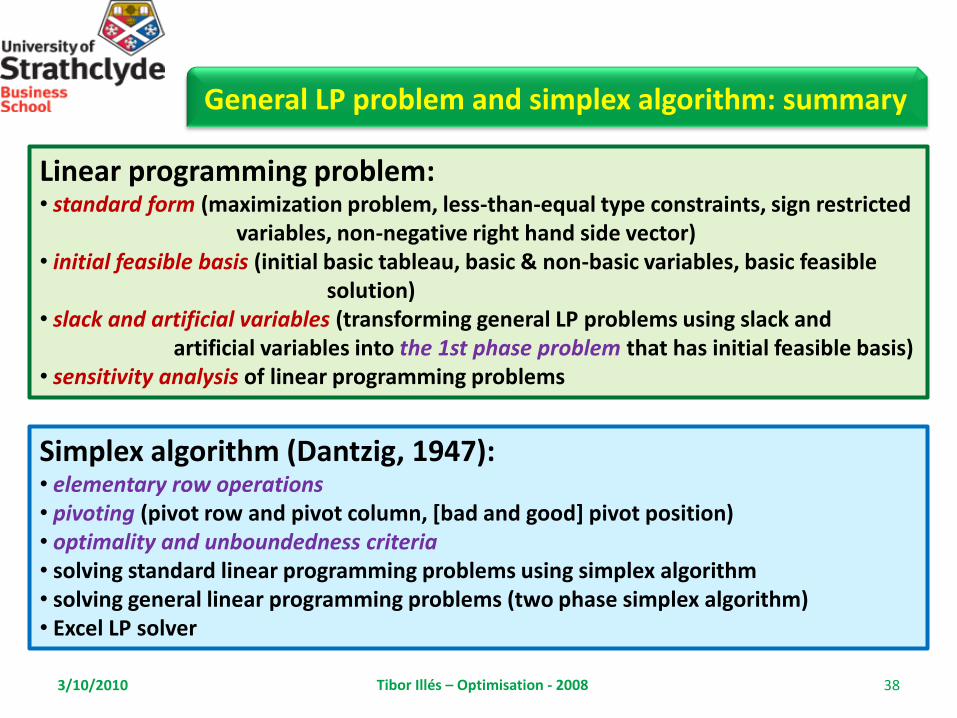
General LP problem and simplex algorithm: summary

Linear programming problem:• standard form (maximization problem, less-than-equal type constraints, sign restricted

variables, non-negative right hand side vector)• initial feasible basis (initial basic tableau, basic & non-basic variables, basic feasible

solution)• slack and artificial variables (transforming general LP problems using slack and

artificial variables into the 1st phase problem that has initial feasible basis)• sensitivity analysis of linear programming problems

Simplex algorithm (Dantzig, 1947):• elementary row operations • pivoting (pivot row and pivot column, [bad and good] pivot position)• optimality and unboundedness criteria• solving standard linear programming problems using simplex algorithm• solving general linear programming problems (two phase simplex algorithm)• Excel LP solver


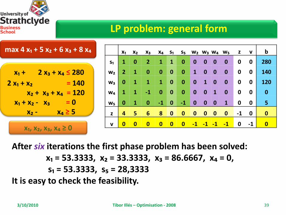
max 4 x₁ + 5 x₂ + 6 x₃ + 8 x₄

x₁ + 2 x₃ + x₄ ≤ 280

2 x₁ + x₂ = 140x₂ + x₃ + x₄ = 120

x₁ + x₂ - x₃ = 0x₂ - x₄ ≥ 5

x₁, x₂, x₃, x₄ ≥ 0


x₁ x₂ x₃ x₄ s₁ s₅ w₂ w₃ w₄ w₅ z v b

s₁ 1 0 2 1 1 0 0 0 0 0 0 0 280

w₂ 2 1 0 0 0 0 1 0 0 0 0 0 140

w₃ 0 1 1 1 0 0 0 1 0 0 0 0 120

w₄ 1 1 -1 0 0 0 0 0 1 0 0 0 0

w₅ 0 1 0 -1 0 -1 0 0 0 1 0 0 5

z 4 5 6 8 0 0 0 0 0 0 -1 0 0

v 0 0 0 0 0 0 -1 -1 -1 -1 0 -1 0

After six iterations the first phase problem has been solved: x₁ = 53.3333, x₂ = 33.3333, x₃ = 86.6667, x₄ = 0, s₁ = 53.3333, s₅ = 28,3333

It is easy to check the feasibility.



x₁ x₂ x₃ x₄ s₁ s₅ w₂ w₃ w₄ w₅ z b

s₁ 0 0 0 0.66667 1 0 -1.3333 -0.333 1.66667 0 0 53.333

x₁ 1 0 0 -0.3333 0 0 0.66667 -0.333 -0.33333 0 0 53.333

s₅ 0 0 0 1.66667 0 1 -0.3333 0.6667 0.66667 -1 0 28.333

x₂ 0 1 0 0.66667 0 0 -0.3333 0.6667 0.66667 0 0 33.333

x₃ 0 0 1 0.33333 0 0 0.33333 0.3333 -0.66667 0 0 86.667

z 0 0 0 4 0 0 -3 -4 2 0 -1 -900

The second phase problem is not optimal. Why ?Pivot position: (3,4). Variable x₄ enters and s₅ leaves the basis.


x₁ x₂ x₃ x₄ s₁ s₅ w₂ w₃ w₄ w₅ z b

s₁ 0 0 0 0 1 -0.4 -1.2 -0.6 1.4 0.4 0 42

x₁ 1 0 0 0 0 0.2 0.6 -0.2 -0.2 -0.2 0 59

x₄ 0 0 0 1 0 0.6 -0.2 0.4 0.4 -0.6 0 17

x₂ 0 1 0 0 0 -0.4 -0.2 0.4 0.4 0.4 0 22

x₃ 0 0 1 0 0 -0.2 0.4 0.2 -0.8 0.2 0 81

z 0 0 0 0 0 -2.4 -2.2 -5.6 0.4 2.4 -1 -968


Is this basic tableau optimal ?Yes, it is optimal ! Why ?Binding constraints are the 2nd – 5th.

Optimal solution is: x₁ = 59, x₂ = 22, x₃ = 81, x₄ = 17, s₁ = 42, s₂ = 0Resource 1 is not fully used, because s₁ = 42, however there is no surplus production from product x₃, because s₅ = 0.The objective function row shows that s₅ has coefficient -2.4, therefore if we relax this constraint to 4 then the objective function value will be 970.4 , however if we increase it to 6, thenthe objective function will decrease to 965.6.



x₁ = 59 + 0.2 = 59.2x₂ = 22 – 0.4 = 21.6x₃ = 81 – 0.2 = 80.8x₄ = 17 + 0.6 = 17.6s₁ = 42 – 0.4 = 41.6s₅ = 0 + 0 = 0

Objective function value:4*59.2 + 5*21.6 + 6*80.8 + 8*17.6 = 970.4

x₁ x₂ x₃ x₄ s₁ s₅ w₂ w₃ w₄ w₅ z b

s₁ 0 0 0 0 1 -0.4 -1.2 -0.6 1.4 0.4 0 42

x₁ 1 0 0 0 0 0.2 0.6 -0.2 -0.2 -0.2 0 59

x₄ 0 0 0 1 0 0.6 -0.2 0.4 0.4 -0.6 0 17

x₂ 0 1 0 0 0 -0.4 -0.2 0.4 0.4 0.4 0 22

x₃ 0 0 1 0 0 -0.2 0.4 0.2 -0.8 0.2 0 81

z 0 0 0 0 0 -2.4 -2.2 -5.6 0.4 2.4 -1 -968



x₁ x₂ x₃ x₄ s₁ s₅ w₂ w₃ w₄ w₅ z b

s₁ 0 0 0 0 1 -0.4 -1.2 -0.6 1.4 0.4 0 42

x₁ 1 0 0 0 0 0.2 0.6 -0.2 -0.2 -0.2 0 59

x₄ 0 0 0 1 0 0.6 -0.2 0.4 0.4 -0.6 0 17

x₂ 0 1 0 0 0 -0.4 -0.2 0.4 0.4 0.4 0 22

x₃ 0 0 1 0 0 -0.2 0.4 0.2 -0.8 0.2 0 81

z 0 0 0 0 0 -2.4 -2.2 -5.6 0.4 2.4 -1 -968

Take into consideration an equality constraint for instance the 2nd.Objective function row in column w₂ contains here as well the opportunity cost.

x₁ = 59 + 0.6 = 59.6x₂ = 22 – 0.2 = 21.8x₃ = 81 + 0.4 = 81.4x₄ = 17 – 0.2 = 16.8s₁ = 42 – 1.2 = 40.8s₅ = 0 + 0 = 0

Increase by 1 unit of the 2nd resource will result the following solution with objective function value of 970.2.How to analyze the case of the 3rd or 4th row ? What does it mean the column of w₄ or w₅ ?


General LP problem: sensitivity analysis

Maximization problems: interpretation of the effects of a 1 unit increase in the RHS of a binding constraint

Constraint type ≤• The relevant columni is that of the associated slack variable.• The opportunity cost coefficient will be negative.• The coefficient indicates the increase in the objective function.• The column coefficients indicates the change in the values of the basic variables.• The maximum change is determined by the smallest ratio of values to negative coefficients in the slack variable column.




Constraint type ≥• The relevant columni is that of the associated surplus (slack) variable. (Surplus variable has -1 coefficient.)• The opportunity cost coefficient will be negative.• The coefficient indicates the decrease in the objective function.• The column coefficients must have their signs reversed (positive) to indicates the change in the values of the basic variables.• The maximum change is determined by the smallest ratio of values to positive coefficients in the slack variable column.




Constraint type =• The relevant columni is that of the associated artificial variable.• The opportunity cost coefficient will be negative.• The coefficient indicates the increase in the objective function.• The column coefficients indicates the change in the values of the basic variables.• The maximum change is determined by the smallest ratio of values to negative coefficients in the relevant column.


An oil refinery produces four types of raw gasoline: alkylate, catalytic-cracked, straight-run and isopentane.Two important characteristics of each gasoline are its performance number PN (indicating antiknock properties) and its vapor pressure RVP (indicating volatility). These two characteristics, together with the production levels in barrels per day, are as follows:

PN RVP Barrels produced

Alkylate 107 5 3814

Catalytic-cracked 93 8 2666

Straight-run 87 4 4016

Isopentane 108 21 1300

A simplified blending problem

These gasolines can be sold either raw at £27.87 per barrel, or blended into aviation gasoline (Avgas A and/or Avgas B).


A simplified blending problem: continue

Quality standards impose certain requirements on the aviation gasolines: these requirements, together with the selling prieces, are as follows:

PN RVP Price per barrel

Avgas A at least 100 at most 7 £42.13

Avgas B at least 91 at most 7 £38.47

The refinery aims for the production plan that yields the largest possible profit. Formulate as a linear programming problem (in standard form).

Remark: The PN and RVP of each mixture are simply weighted averages of the PNs and RVPs of its constituents.


Model for the blending problem

Alkylate Catalytic-cracked

Straight-runIsopentane

Avgas A

Avgas B

x₁ x₂

x₃

x₄

a

b

x₁₁

x₂₁

x₃₁x₄₁

x₁₂x₂₂

x₃₂x₄₂


Linear programming model for blending

Decision variables

Alkylate x₁Catalytic-cracked x₂Straight-run x₃Isopentane x₄Avgas A aAvgas B b

Avgas A Avgas BAlkylate x₁₁ x₁₂Catalytic-cracked x₂₁ x₂₂Straight-run x₃₁ x₃₂Isopentane x₄₁ x₄₂

The decision variables are either sign restricted or bounded variables.

0 ≤ x₁ ≤ 3814, 0 ≤ x₂ ≤ 2666, 0 ≤ x₃ ≤ 4016, 0 ≤ x₄ ≤ 1300


Bounds, flow and qualitative constraints

x₁₁ + x₁₂ + s₁ = x₁x₂₁ + x₂₂ + s₂ = x₂x₃₁ + x₃₂ + s₃ = x₃x₄₁ + x₄₂ + s₄ = x₄

x₁₁ + x₂₁ + x₃₁ + x₄₁ = ax₁₂ + x₂₂ + x₃₂ + x₄₂ = b

100 a ≤ 107 x₁₁ + 93 x₂₁ + 87 x₃₁ + 108 x₄₁ 91 b ≤ 107 x₁₂ + 93 x₂₂ + 87 x₃₂ + 108 x₄₂

5 x₁₁ + 8 x₂₁ + 4 x₃₁ + 21 x₄₁ ≤ 7 a5 x₁₂ + 8 x₂₂ + 4 x₃₂ + 21 x₄₂ ≤ 7 b

max 42.13 a + 38.47 b + 27.87 (s₁ + s₂ + s₃ + s₄)


a b x₁ x₂ x₃ x₄ x₁₁ x₂₁ x₃₁ x₄₁ x₁₂ x₂₂ x₃₂ x₄₂ s₁ s₂ s₃ s₄ RHS

0 0 0 0 0 0 0 0 0 0 0 0 0 0 0 0 0 0

0 0 -1 0 0 0 1 0 0 0 1 0 0 0 1 0 0 0 0 0

0 0 0 -1 0 0 0 1 0 0 0 1 0 0 0 1 0 0 0 0

0 0 0 0 -1 0 0 0 1 0 0 0 1 0 0 0 1 0 0 0

0 0 0 0 0 -1 0 0 0 1 0 0 0 1 0 0 0 1 0 0

-1 0 0 0 0 0 1 1 1 1 0 0 0 0 0 0 0 0 0 0

0 -1 0 0 0 0 0 0 0 0 1 1 1 1 0 0 0 0 0 0

-100 0 0 0 0 0 107 93 87 108 0 0 0 0 0 0 0 0 0≥ 0

0 -91 0 0 0 0 0 0 0 0 107 93 87 108 0 0 0 0 0≥ 0

-7 0 0 0 0 0 5 8 4 21 0 0 0 0 0 0 0 0 0≤ 0

0 -7 0 0 0 0 0 0 0 0 5 8 4 21 0 0 0 0 0≤ 0

0 0 1 0 0 0 0 0 0 0 0 0 0 0 0 0 0 0 0≤ 3814

0 0 0 1 0 0 0 0 0 0 0 0 0 0 0 0 0 0 0≤ 2666

0 0 0 0 1 0 0 0 0 0 0 0 0 0 0 0 0 0 0≤ 4016

0 0 0 0 0 1 0 0 0 0 0 0 0 0 0 0 0 0 0≤ 1300

42.13 38.47 0 0 0 0 0 0 0 0 0 0 0 0 27.87 27.87 27.87 27.87 0

Linear programming problem: Excel form

The LP problem is primal and dual degenerate !


a b x₁ x₂ x₃ x₄ x₁₁ x₂₁ x₃₁ x₄₁ x₁₂ x₂₂ x₃₂ x₄₂ s₁ s₂ s₃ s₄ RHS

7883 3828 3814 2666 4016 1300 3814 1602.666667 1676.666667 790 0 1063.333333 2339.333333 425 0 0 0 85

0 0 -1 0 0 0 1 0 0 0 1 0 0 0 1 0 0 0 0 0

0 0 0 -1 0 0 0 1 0 0 0 1 0 0 0 1 0 0 2.27E-13 0

0 0 0 0 -1 0 0 0 1 0 0 0 1 0 0 0 1 0 0 0

0 0 0 0 0 -1 0 0 0 1 0 0 0 1 0 0 0 1 -1.6E-13 0

-1 0 0 0 0 0 1 1 1 1 0 0 0 0 0 0 0 0 1.02E-12 0

0 -1 0 0 0 0 0 0 0 0 1 1 1 1 0 0 0 0 2.27E-13 0

-100 0 0 0 0 0 107 93 87 108 0 0 0 0 0 0 0 0 2.04E-10≥ 0

0 -91 0 0 0 0 0 0 0 0 107 93 87 108 0 0 0 0 5.82E-11≥ 0

-7 0 0 0 0 0 5 8 4 21 0 0 0 0 0 0 0 0 1.09E-11≤ 0

0 -7 0 0 0 0 0 0 0 0 5 8 4 21 0 0 0 0 -3.6E-12≤ 0

0 0 1 0 0 0 0 0 0 0 0 0 0 0 0 0 0 0 3814≤ 3814

0 0 0 1 0 0 0 0 0 0 0 0 0 0 0 0 0 0 2666≤ 2666

0 0 0 0 1 0 0 0 0 0 0 0 0 0 0 0 0 0 4016≤ 4016

0 0 0 0 0 1 0 0 0 0 0 0 0 0 0 0 0 0 1300≤ 1300

42.13 38.47 0 0 0 0 0 0 0 0 0 0 0 0 27.87 27.87 27.87 27.87 481742.9


Optimal solution of the blending problem

Alkylate Catalytic-cracked

Straight-runIsopentane

Avgas A

Avgas B

3814 2666

4016

1215

7883

3828

3814

1602.667

1676.667

790

01063.33

2339.33

425


100 a ≤ 107 x₁₁ + 93 x₂₁ + 87 x₃₁ + 108 x₄₁ 91 b ≤ 107 x₁₂ + 93 x₂₂ + 87 x₃₂ + 108 x₄₂

5 x₁₁ + 8 x₂₁ + 4 x₃₁ + 21 x₄₁ ≤ 7 a5 x₁₂ + 8 x₂₂ + 4 x₃₂ + 21 x₄₂ ≤ 7 b

PNa a = 107 x₁₁ + 93 x₂₁ + 87 x₃₁ + 108 x₄₁ PNb b = 107 x₁₂ + 93 x₂₂ + 87 x₃₂ + 108 x₄₂

5 x₁₁ + 8 x₂₁ + 4 x₃₁ + 21 x₄₁ = RVPa a5 x₁₂ + 8 x₂₂ + 4 x₃₂ + 21 x₄₂ = RVPb b

99.8 ≤ PNa ≤ 102, 90.8 ≤ PNb ≤ 93, 6.5 ≤ RVPa, RVPb ≤ 7.5

New qualitative variables: bilinear terms


Resource allocation problem

Ajax Ltd. manufactures and sells three types of computer: α-PC, β-NB and γ-WS. For the moment we assume that all production during the week can and will be sold immediately.

α-PC β-NB γ-WS

Net profit 160 210 310 in £s

Labour 10 15 20 in hours

purchasing components, producing computer cases, and assembling and testing computer. This week, 120 hours are available on the A-line test equipment where assembled α-PCs and β-NBs are tested, and 48 hours are available on the C-line test equipment where assembled γ-WSs are tested. The testing of each computer takes 1 hour. In addition, production is constrained by the availability of 2000 labor hours for product assembly.

Net profit equals the sales price of each computer minus the direct cost of


Resource allocation model

a – the number of α-PCsb – the number of β-NBs c – the number of γ-WSs

Decision variables max 160 a + 210 b + 310 c10 a + 15 b + 20 c ≤ 2000

a + b ≤ 120c ≤ 48

a, b, c ≥ 0


$C$9 a 0 120

$D$9 b 0 0

$E$9 c 0 40


$G$11 production 2000 $G$11<=$H$11 Binding 0

$G$12 test1 120 $G$12<=$H$12 Binding 0

$G$13 test2 40 $G$13<=$H$13 Not Binding 8



$C$9 a 120 0 160 1E+30 5

$D$9 b 0 -27.5 210 27.5 1E+30

$E$9 c 40 0 310 10 110



$G$11 production 2000 15.5 2000 160 800

$G$12 test1 120 5 120 80 16

$G$13 test2 40 0 48 1E+30 8Cell Name Original Value Final Value

$G$15 objective 0 31600


Shadow price

A fundamental ingredient in the economic analysis of an LP model is the shadow price associated with each constraint, which is defined as the change in the optimal value of the objective function if the right-hand side of the constraint is increased by one unit. For reasons of symmetry, it is also defined as the change in the optimal value of the objective function if the right-hand side of the constraint is decreased by one unit.


a b c120 0 39.95

production 10 15 20 1999 1999test1 1 1 0 120 120test2 0 0 1 39.95 48

objective 160 210 310 31584.5

1 unit decrease in the right-hand side

Shadow price of the 1st constraint is 15.5

Change in the objective function value is

31584.5 = 31600 – 15.5

Non integer optimal solution !

Shadow price: practical application

Rounding the solution to the

nearest integer ?


a b c120 0 39.95

production 10 15 20 1999 1999test1 1 1 0 120 120test2 0 0 1 39.95 48

objective 160 210 310 31584.5

Rounding to the nearest integer solution

a b c

solution 1 120 0 39.95

solution 2 120 0 40solution 3 120 0 39

solution 1 solution 2 solution 3

1999 2000 1980 1999

120 120 120 120

39.95 40 39 48

solution 1 – optimal solution of the linear programming problem with real variables

solution 2 – integer solution, but infeasible

solution 3 – it is a feasible, integer solution of the LP problem. Optimality of the integer solution ?


Resource allocation problem: dual version

The Immense Computer Co. is experiencing a rapid growth in sales. As a result, Immense has insufficient capacity for testing and assembling their computers, and the director of purchasing is looking to rent capacity from other smaller, companies. She is considering approaching Ajax to offer to rent its capacity on a weekly basis.

In particular, she wishes to determine nonnegative prices per hour of A-line test capacity, nonnegative prices per hour of C-line test capacity and nonnegative prices per hour of labour capacity to offer Ajax that will induce Ajax into agreeing to rent its resources rather than to use them in the manufacture of its own products. At the same time she wishes to pay the least amount for these resources. A number of large manufacturing firms are concered with the economic viability of their small suppliers.

α-PC β-NB γ-WS Capacity


Labour 10 15 20 in hours 2000

A-line 1 1 0 in hours 120

C-line 0 0 1 in hours 48


Resource allocation model: dual problem

Decision variables

u – price per hour of A-line testv – price per hour of C-line testz – price per hour of labour

min 120 u + 48 v + 2000 zu + 10 z ≥ 160u + 15 z ≥ 210

v + 20 z ≥ 310u, v, z ≥ 0

α-PC β-NB γ-WS Capacity


Labour 10 15 20 in hours 2000

A-line 1 1 0 in hours 120

C-line 0 0 1 in hours 48


$C$19 u 0 15.5

$D$19 v 0 5

$E$19 z 0 0


$G$21 160 $G$21>=$H$21 Binding 0

$G$22 237.5 $G$22>=$H$22 Not Binding 27.5

$G$23 310 $G$23>=$H$23 Binding 0



$C$19 u 15.5 0 2000 160 800

$D$19 v 5 0 120 80 16

$E$19 z 0 8 48 1E+30 8



$G$21 160 120 160 1E+30 5

$G$22 237.5 0 210 27.5 1E+30

$G$23 310 40 310 10 110


Integerality of the solution(s) of LP problems

max 160 a + 210 b + 310 c10 a + 15 b + 20 c ≤ 2000

a + b ≤ 120c ≤ 48

a, b, c ≥ 0

min 120 u + 48 v + 2000 zu + 10 z ≥ 160u + 15 z ≥ 210

v + 20 z ≥ 310u, v, z ≥ 0

Name Final Value

a 120

b 0

c 40

Name Final Value

u 15.5

v 5

z 0

solution

a 1999 1999

b 120 120

c 39.95 48

Why these solutions are not

integer ?Explanation lies in deeper

understanding of mathematics behind these models !


Standard primal – dual linear programming problem

primal objective coefficient = dual constraint R.H. sidedual objective coefficient = primal constraint R.H. side

primal solution = dual shadow pricedual solution = primal shadow price

primal slack = dual reduced costdual slack = - primal reduced cost

Mathematics !

Shadow price & reduced cost


Resource allocation model: modification

Since the full capacity of C-line test equipment were not used in the optimal production plan, the engineers made an invention and as a consequence of this α-PCs can be tested on C-line as well, but such a test takes 1.5 hours. Modify the model for this case.

max 160 a + 210 b + 310 ca – a₂ – a₁ = 0

10 a + 15 b + 20 c ≤ 2000a₁ + b ≤ 120

1.5 a₂ + c ≤ 48a, a₁, a₂, b, c ≥ 0


a1 a2 a b c120 8 128 0 36

a-pcs -1 -1 1 0 0 0 0production 0 0 10 15 20 2000 2000test1 1 0 0 1 0 120 120test2 0 1.5 0 0 1 48 48

objective 0 0 160 210 310 31640

Solution of the modified model

The optimal solution of the modified resource allocation problem is

optimal and all resources are fully used.

Furthermore the solution is integer !


Resource allocation: outsourcing

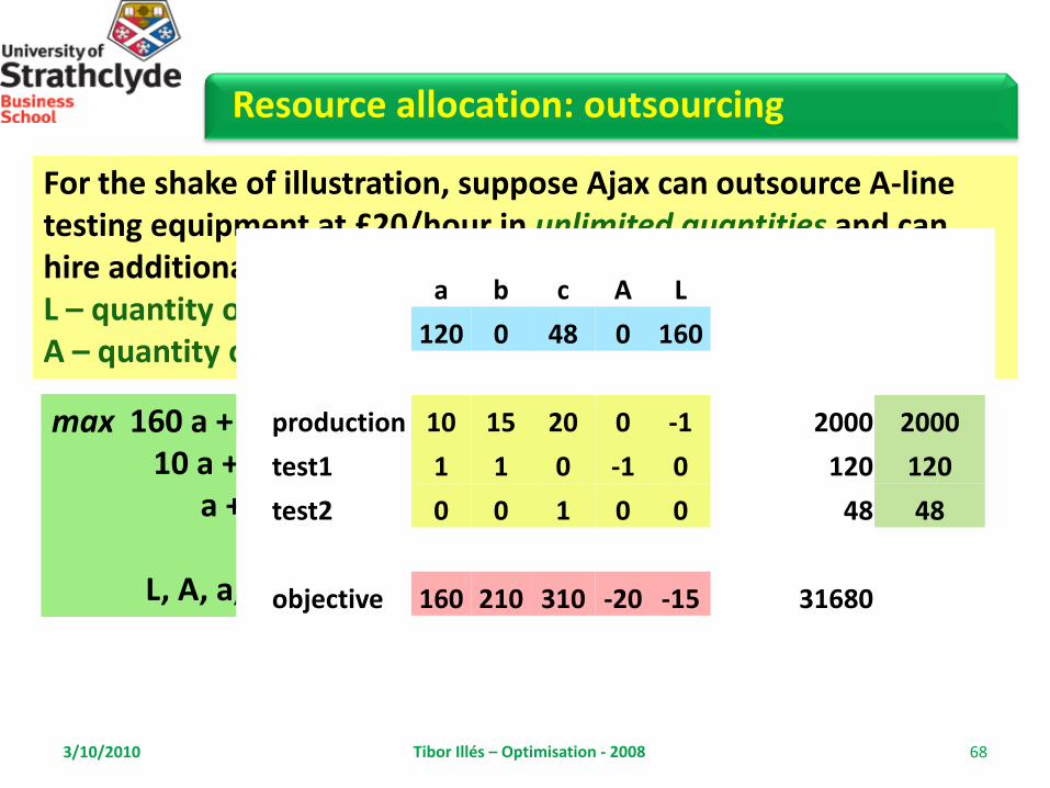
For the shake of illustration, suppose Ajax can outsource A-line testing equipment at £20/hour in unlimited quantities and can hire additional labour at £15/hour in unlimited quantities. LetL – quantity of rented labour hoursA – quantity of outsourced A-line test hours

max 160 a + 210 b + 310 c – 20 A – 15 L 10 a + 15 b + 20 c ≤ 2000 + L

a + b ≤ 120 + Ac ≤ 48

L, A, a, b, c ≥ 0

a b c A L

120 0 48 0 160

production 10 15 20 0 -1 2000 2000

test1 1 1 0 -1 0 120 120

test2 0 0 1 0 0 48 48

objective 160 210 310 -20 -15 31680


Multiperiod Resource Allocation Problem

After reviewing the optimal assembly plan given by the optimal solution (120, 0, 40) of the previous LP model the Ajax’ marketing manager doubts that his organization can sell 120 units of α-PCs next week. Moreover, he is concerned that the plan does not call for the assembly of any β-NBs. Even if the profit margin from β-NBs is smaller relative to the other two pruducts, the marketing manager feels strongly that it must be included in Ajax’ product line.Thus he requests instead that the production manager develop a 4-week production strategy based on the sales forecasts shown

Week 1 Week 2 Week 3 Week 4

α-PC [20,60] [20,80] [20,120] [20,140]

β-NB [20,40] [20,40] [20,40] [20,40]

γ-WS [20,50] [20,40] [20,30] [20,70]

Because Ajax has capital tied up in products, carrying costs must be charged for items held in inventory. These carrying costs £4 per week for

each α-PC, £5 per week for each β-NB, and £9 per week for each γ-WS. Initial inventory at this week equals 22 α-PCs, 42 β-NBs, and 36 γ-WSs. For each product, these balance equations are of the form

I(t) = I(t-1) + P(t) – S(t)


Multiperiod Resource Allocation Model

10 aj + 15 bj + 20 cj ≤ 2000aj + bj ≤ 120

cj ≤ 48aj, bj, cj ≥ 0 (j = 1, 2, 3, 4)

Production constraints

160 Saj + 210 Sbj + 310 Scj - 4 Iaj - 5 Ibj - 9 Icj = zj, zj ≥ 0, (j = 1, 2, 3, 4)

Iaj = Iaj-1 + aj – Saj, Laj ≤ Saj ≤ Uaj

Ibj = Ibj-1 + bj – Sbj, Lbj ≤ Sbj ≤ Ubj

Icj = Icj-1 + cj – Scj, Lcj ≤ Scj ≤ Ucj

Iaj, Ibj, Icj, Saj, Sbj, Scj ≥ 0, (j = 1, 2, 3, 4)

Inventory constraints

max z₁ + z₂ + z₃ + z₄ Profit constraints



Week 1


Week 2


Week 1


Week 3


Week 2

Profit constraintsWeek 1



Sp₁

p₁ - Sp₁

Sp₂ Sp₃

p₂ - Sp₂

Ip₁ Ip2

Multiperiod Resource Allocation Model


a₁ b₁ c₁ a₂ b₂ c₂ a₃ b₃ c₃ a₄ b₄ c₄ Ia₁ Ib₁ Ic₁ Ia₂ Ib₂ Ic₂ Ia₃ Ib₃ Ic₃ Ia₄ Ib₄ Ic₄ Sa₁ Sb₁ Sc₁ Sa₂ Sb₂ Sc₂ Sa₃ Sb₃ Sc₃ Sa₄ Sb₄ Sc₄ z₁ z₂ z₃ z₄

0 0 0 0 0 0 0 0 0 0 0 0 0 0 0 0 0 0 0 0 0 0 0 0 0 0 0 0 0 0 0 0 0 0 0 0 0 0 0 0

production₁ 10 15 20 0 0 0 0 0 0 0 0 0 0 0 0 0 0 0 0 0 0 0 0 0 0 0 0 0 0 0 0 0 0 0 0 0 0 0 0 0 0 ≤ 2000

test1₁ 1 1 0 0 0 0 0 0 0 0 0 0 0 0 0 0 0 0 0 0 0 0 0 0 0 0 0 0 0 0 0 0 0 0 0 0 0 0 0 0 0 ≤ 120

test2₁ 0 0 1 0 0 0 0 0 0 0 0 0 0 0 0 0 0 0 0 0 0 0 0 0 0 0 0 0 0 0 0 0 0 0 0 0 0 0 0 0 0 ≤ 48

production₂ 0 0 0 10 15 20 0 0 0 0 0 0 0 0 0 0 0 0 0 0 0 0 0 0 0 0 0 0 0 0 0 0 0 0 0 0 0 0 0 0 0 ≤ 2000

test1₂ 0 0 0 1 1 0 0 0 0 0 0 0 0 0 0 0 0 0 0 0 0 0 0 0 0 0 0 0 0 0 0 0 0 0 0 0 0 0 0 0 0 ≤ 120

test2₂ 0 0 0 0 0 1 0 0 0 0 0 0 0 0 0 0 0 0 0 0 0 0 0 0 0 0 0 0 0 0 0 0 0 0 0 0 0 0 0 0 0 ≤ 48

production₃ 0 0 0 0 0 0 10 15 20 0 0 0 0 0 0 0 0 0 0 0 0 0 0 0 0 0 0 0 0 0 0 0 0 0 0 0 0 0 0 0 0 ≤ 2000

test1₃ 0 0 0 0 0 0 1 1 0 0 0 0 0 0 0 0 0 0 0 0 0 0 0 0 0 0 0 0 0 0 0 0 0 0 0 0 0 0 0 0 0 ≤ 120

test2₃ 0 0 0 0 0 0 0 0 1 0 0 0 0 0 0 0 0 0 0 0 0 0 0 0 0 0 0 0 0 0 0 0 0 0 0 0 0 0 0 0 0 ≤ 48

production₄ 0 0 0 0 0 0 0 0 0 10 15 20 0 0 0 0 0 0 0 0 0 0 0 0 0 0 0 0 0 0 0 0 0 0 0 0 0 0 0 0 0 ≤ 2000

test1₄ 0 0 0 0 0 0 0 0 0 1 1 0 0 0 0 0 0 0 0 0 0 0 0 0 0 0 0 0 0 0 0 0 0 0 0 0 0 0 0 0 0 ≤ 120

test2₄ 0 0 0 0 0 0 0 0 0 0 0 1 0 0 0 0 0 0 0 0 0 0 0 0 0 0 0 0 0 0 0 0 0 0 0 0 0 0 0 0 0 ≤ 48

inventory-a₁ -1 0 0 0 0 0 0 0 0 0 0 0 1 0 0 0 0 0 0 0 0 0 0 0 1 0 0 0 0 0 0 0 0 0 0 0 0 0 0 0 0 equal 22

inventory-b₁ 0 -1 0 0 0 0 0 0 0 0 0 0 0 1 0 0 0 0 0 0 0 0 0 0 0 1 0 0 0 0 0 0 0 0 0 0 0 0 0 0 0 equal 42

inventory-c₁ 0 0 -1 0 0 0 0 0 0 0 0 0 0 0 1 0 0 0 0 0 0 0 0 0 0 0 1 0 0 0 0 0 0 0 0 0 0 0 0 0 0 equal 36

inventory-a₂ 0 0 0 -1 0 0 0 0 0 0 0 0 -1 0 0 1 0 0 0 0 0 0 0 0 0 0 0 1 0 0 0 0 0 0 0 0 0 0 0 0 0 equal 0

inventory-b₂ 0 0 0 0 -1 0 0 0 0 0 0 0 0 -1 0 0 1 0 0 0 0 0 0 0 0 0 0 0 1 0 0 0 0 0 0 0 0 0 0 0 0 equal 0

inventory-c₂ 0 0 0 0 0 -1 0 0 0 0 0 0 0 0 -1 0 0 1 0 0 0 0 0 0 0 0 0 0 0 1 0 0 0 0 0 0 0 0 0 0 0 equal 0

inventory-a₃ 0 0 0 0 0 0 -1 0 0 0 0 0 0 0 0 -1 0 0 1 0 0 0 0 0 0 0 0 0 0 0 1 0 0 0 0 0 0 0 0 0 0 equal 0

inventory-b₃ 0 0 0 0 0 0 0 -1 0 0 0 0 0 0 0 0 -1 0 0 1 0 0 0 0 0 0 0 0 0 0 0 1 0 0 0 0 0 0 0 0 0 equal 0

inventory-c₃ 0 0 0 0 0 0 0 0 -1 0 0 0 0 0 0 0 0 -1 0 0 1 0 0 0 0 0 0 0 0 0 0 0 1 0 0 0 0 0 0 0 0 equal 0

inventory-a₄ 0 0 0 0 0 0 0 0 0 -1 0 0 0 0 0 0 0 0 -1 0 0 1 0 0 0 0 0 0 0 0 0 0 0 1 0 0 0 0 0 0 0 equal 0

inventory-b₄ 0 0 0 0 0 0 0 0 0 0 -1 0 0 0 0 0 0 0 0 -1 0 0 1 0 0 0 0 0 0 0 0 0 0 0 1 0 0 0 0 0 0 equal 0

inventory-c₄ 0 0 0 0 0 0 0 0 0 0 0 -1 0 0 0 0 0 0 0 0 -1 0 0 1 0 0 0 0 0 0 0 0 0 0 0 1 0 0 0 0 0 equal 0

obj-week₁ 0 0 0 0 0 0 0 0 0 0 0 0 0 0 0 0 0 0 0 0 0 0 0 0 160 210 130 0 0 0 0 0 0 0 0 0 -1 0 0 0 0 equal 622

obj-week₂ 0 0 0 0 0 0 0 0 0 0 0 0 -4 -5 -9 0 0 0 0 0 0 0 0 0 0 0 0 160 210 130 0 0 0 0 0 0 0 -1 0 0 0 equal 0

obj-week₃ 0 0 0 0 0 0 0 0 0 0 0 0 0 0 0 -4 -5 -9 0 0 0 0 0 0 0 0 0 0 0 0 160 210 130 0 0 0 0 0 -1 0 0 equal 0

obj-week₄ 0 0 0 0 0 0 0 0 0 0 0 0 0 0 0 0 0 0 -4 -5 -9 0 0 0 0 0 0 0 0 0 0 0 0 160 210 130 0 0 0 -1 0 equal 0

lower bounds 0 0 0 0 0 0 0 0 0 0 0 0 0 0 0 0 0 0 0 0 0 0 0 0 1 0 0 0 0 0 0 0 0 0 0 0 0 0 0 0 0 ≥ 20

lower bounds 0 0 0 0 0 0 0 0 0 0 0 0 0 0 0 0 0 0 0 0 0 0 0 0 0 1 0 0 0 0 0 0 0 0 0 0 0 0 0 0 0 ≥ 20

lower bounds 0 0 0 0 0 0 0 0 0 0 0 0 0 0 0 0 0 0 0 0 0 0 0 0 0 0 1 0 0 0 0 0 0 0 0 0 0 0 0 0 0 ≥ 20

lower bounds 0 0 0 0 0 0 0 0 0 0 0 0 0 0 0 0 0 0 0 0 0 0 0 0 0 0 0 1 0 0 0 0 0 0 0 0 0 0 0 0 0 ≥ 20

lower bounds 0 0 0 0 0 0 0 0 0 0 0 0 0 0 0 0 0 0 0 0 0 0 0 0 0 0 0 0 1 0 0 0 0 0 0 0 0 0 0 0 0 ≥ 20

lower bounds 0 0 0 0 0 0 0 0 0 0 0 0 0 0 0 0 0 0 0 0 0 0 0 0 0 0 0 0 0 1 0 0 0 0 0 0 0 0 0 0 0 ≥ 20

lower bounds 0 0 0 0 0 0 0 0 0 0 0 0 0 0 0 0 0 0 0 0 0 0 0 0 0 0 0 0 0 0 1 0 0 0 0 0 0 0 0 0 0 ≥ 20

lower bounds 0 0 0 0 0 0 0 0 0 0 0 0 0 0 0 0 0 0 0 0 0 0 0 0 0 0 0 0 0 0 0 1 0 0 0 0 0 0 0 0 0 ≥ 20

lower bounds 0 0 0 0 0 0 0 0 0 0 0 0 0 0 0 0 0 0 0 0 0 0 0 0 0 0 0 0 0 0 0 0 1 0 0 0 0 0 0 0 0 ≥ 20

lower bounds 0 0 0 0 0 0 0 0 0 0 0 0 0 0 0 0 0 0 0 0 0 0 0 0 0 0 0 0 0 0 0 0 0 1 0 0 0 0 0 0 0 ≥ 20

lower bounds 0 0 0 0 0 0 0 0 0 0 0 0 0 0 0 0 0 0 0 0 0 0 0 0 0 0 0 0 0 0 0 0 0 0 1 0 0 0 0 0 0 ≥ 20

lower bounds 0 0 0 0 0 0 0 0 0 0 0 0 0 0 0 0 0 0 0 0 0 0 0 0 0 0 0 0 0 0 0 0 0 0 0 1 0 0 0 0 0 ≥ 20

upper bounds 0 0 0 0 0 0 0 0 0 0 0 0 0 0 0 0 0 0 0 0 0 0 0 0 1 0 0 0 0 0 0 0 0 0 0 0 0 0 0 0 0 ≤ 60

upper bounds 0 0 0 0 0 0 0 0 0 0 0 0 0 0 0 0 0 0 0 0 0 0 0 0 0 1 0 0 0 0 0 0 0 0 0 0 0 0 0 0 0 ≤ 40

upper bounds 0 0 0 0 0 0 0 0 0 0 0 0 0 0 0 0 0 0 0 0 0 0 0 0 0 0 1 0 0 0 0 0 0 0 0 0 0 0 0 0 0 ≤ 50

upper bounds 0 0 0 0 0 0 0 0 0 0 0 0 0 0 0 0 0 0 0 0 0 0 0 0 0 0 0 1 0 0 0 0 0 0 0 0 0 0 0 0 0 ≤ 80

upper bounds 0 0 0 0 0 0 0 0 0 0 0 0 0 0 0 0 0 0 0 0 0 0 0 0 0 0 0 0 1 0 0 0 0 0 0 0 0 0 0 0 0 ≤ 40

upper bounds 0 0 0 0 0 0 0 0 0 0 0 0 0 0 0 0 0 0 0 0 0 0 0 0 0 0 0 0 0 1 0 0 0 0 0 0 0 0 0 0 0 ≤ 40

upper bounds 0 0 0 0 0 0 0 0 0 0 0 0 0 0 0 0 0 0 0 0 0 0 0 0 0 0 0 0 0 0 1 0 0 0 0 0 0 0 0 0 0 ≤ 120

upper bounds 0 0 0 0 0 0 0 0 0 0 0 0 0 0 0 0 0 0 0 0 0 0 0 0 0 0 0 0 0 0 0 1 0 0 0 0 0 0 0 0 0 ≤ 40

upper bounds 0 0 0 0 0 0 0 0 0 0 0 0 0 0 0 0 0 0 0 0 0 0 0 0 0 0 0 0 0 0 0 0 1 0 0 0 0 0 0 0 0 ≤ 30

upper bounds 0 0 0 0 0 0 0 0 0 0 0 0 0 0 0 0 0 0 0 0 0 0 0 0 0 0 0 0 0 0 0 0 0 1 0 0 0 0 0 0 0 ≤ 140

upper bounds 0 0 0 0 0 0 0 0 0 0 0 0 0 0 0 0 0 0 0 0 0 0 0 0 0 0 0 0 0 0 0 0 0 0 1 0 0 0 0 0 0 ≤ 40

upper bounds 0 0 0 0 0 0 0 0 0 0 0 0 0 0 0 0 0 0 0 0 0 0 0 0 0 0 0 0 0 0 0 0 0 0 0 1 0 0 0 0 0 ≤ 70

obj function 0 0 0 0 0 0 0 0 0 0 0 0 0 0 0 0 0 0 0 0 0 0 0 0 0 0 0 0 0 0 0 0 0 0 0 0 1 1 1 1 0

Structure of the multi-period model


Solution of the multi-period model

a₁ b₁ c₁ a₂ b₂ c₂ a₃ b₃ c₃ a₄ b₄ c₄ Ia₁ Ib₁ Ic₁ Ia₂ Ib₂ Ic₂ Ia₃ Ib₃ Ic₃ Ia₄ Ib₄ Ic₄ Sa₁ Sb₁ Sc₁ Sa₂ Sb₂ Sc₂ Sa₃ Sb₃ Sc₃ Sa₄ Sb₄ Sc₄ z₁ z₂ z₃ z₄

38 82 20 98 22 35 106 14 36 120 0 40 0 84 5 18 66 0 4 40 6 0 0 0 60 40 50 80 40 40 120 40 30 124 40 46 23878 25930.5 31098 34010.5

production₁ 10 15 20 0 0 0 0 0 0 0 0 0 0 0 0 0 0 0 0 0 0 0 0 0 0 0 0 0 0 0 0 0 0 0 0 0 0 0 0 0 2000 ≤ 2000

test1₁ 1 1 0 0 0 0 0 0 0 0 0 0 0 0 0 0 0 0 0 0 0 0 0 0 0 0 0 0 0 0 0 0 0 0 0 0 0 0 0 0 120 ≤ 120

test2₁ 0 0 1 0 0 0 0 0 0 0 0 0 0 0 0 0 0 0 0 0 0 0 0 0 0 0 0 0 0 0 0 0 0 0 0 0 0 0 0 0 19.5 ≤ 48

production₂ 0 0 0 10 15 20 0 0 0 0 0 0 0 0 0 0 0 0 0 0 0 0 0 0 0 0 0 0 0 0 0 0 0 0 0 0 0 0 0 0 2000 ≤ 2000

test1₂ 0 0 0 1 1 0 0 0 0 0 0 0 0 0 0 0 0 0 0 0 0 0 0 0 0 0 0 0 0 0 0 0 0 0 0 0 0 0 0 0 120 ≤ 120

test2₂ 0 0 0 0 0 1 0 0 0 0 0 0 0 0 0 0 0 0 0 0 0 0 0 0 0 0 0 0 0 0 0 0 0 0 0 0 0 0 0 0 34.5 ≤ 48

production₃ 0 0 0 0 0 0 10 15 20 0 0 0 0 0 0 0 0 0 0 0 0 0 0 0 0 0 0 0 0 0 0 0 0 0 0 0 0 0 0 0 2000 ≤ 2000

test1₃ 0 0 0 0 0 0 1 1 0 0 0 0 0 0 0 0 0 0 0 0 0 0 0 0 0 0 0 0 0 0 0 0 0 0 0 0 0 0 0 0 120 ≤ 120

test2₃ 0 0 0 0 0 0 0 0 1 0 0 0 0 0 0 0 0 0 0 0 0 0 0 0 0 0 0 0 0 0 0 0 0 0 0 0 0 0 0 0 36.5 ≤ 48

production₄ 0 0 0 0 0 0 0 0 0 10 15 20 0 0 0 0 0 0 0 0 0 0 0 0 0 0 0 0 0 0 0 0 0 0 0 0 0 0 0 0 2000 ≤ 2000

test1₄ 0 0 0 0 0 0 0 0 0 1 1 0 0 0 0 0 0 0 0 0 0 0 0 0 0 0 0 0 0 0 0 0 0 0 0 0 0 0 0 0 120 ≤ 120

test2₄ 0 0 0 0 0 0 0 0 0 0 0 1 0 0 0 0 0 0 0 0 0 0 0 0 0 0 0 0 0 0 0 0 0 0 0 0 0 0 0 0 40 ≤ 48

inventory-a₁ -1 0 0 0 0 0 0 0 0 0 0 0 1 0 0 0 0 0 0 0 0 0 0 0 1 0 0 0 0 0 0 0 0 0 0 0 0 0 0 0 22 equal 22

inventory-b₁ 0 -1 0 0 0 0 0 0 0 0 0 0 0 1 0 0 0 0 0 0 0 0 0 0 0 1 0 0 0 0 0 0 0 0 0 0 0 0 0 0 42 equal 42

inventory-c₁ 0 0 -1 0 0 0 0 0 0 0 0 0 0 0 1 0 0 0 0 0 0 0 0 0 0 0 1 0 0 0 0 0 0 0 0 0 0 0 0 0 36 equal 36

inventory-a₂ 0 0 0 -1 0 0 0 0 0 0 0 0 -1 0 0 1 0 0 0 0 0 0 0 0 0 0 0 1 0 0 0 0 0 0 0 0 0 0 0 0 -5.7E-14 equal 0

inventory-b₂ 0 0 0 0 -1 0 0 0 0 0 0 0 0 -1 0 0 1 0 0 0 0 0 0 0 0 0 0 0 1 0 0 0 0 0 0 0 0 0 0 0 2.63E-13 equal 0

inventory-c₂ 0 0 0 0 0 -1 0 0 0 0 0 0 0 0 -1 0 0 1 0 0 0 0 0 0 0 0 0 0 0 1 0 0 0 0 0 0 0 0 0 0 7.53E-13 equal 0

inventory-a₃ 0 0 0 0 0 0 -1 0 0 0 0 0 0 0 0 -1 0 0 1 0 0 0 0 0 0 0 0 0 0 0 1 0 0 0 0 0 0 0 0 0 1.42E-14 equal 0

inventory-b₃ 0 0 0 0 0 0 0 -1 0 0 0 0 0 0 0 0 -1 0 0 1 0 0 0 0 0 0 0 0 0 0 0 1 0 0 0 0 0 0 0 0 -5.9E-13 equal 0

inventory-c₃ 0 0 0 0 0 0 0 0 -1 0 0 0 0 0 0 0 0 -1 0 0 1 0 0 0 0 0 0 0 0 0 0 0 1 0 0 0 0 0 0 0 7.82E-14 equal 0

inventory-a₄ 0 0 0 0 0 0 0 0 0 -1 0 0 0 0 0 0 0 0 -1 0 0 1 0 0 0 0 0 0 0 0 0 0 0 1 0 0 0 0 0 0 3.69E-13 equal 0

inventory-b₄ 0 0 0 0 0 0 0 0 0 0 -1 0 0 0 0 0 0 0 0 -1 0 0 1 0 0 0 0 0 0 0 0 0 0 0 1 0 0 0 0 0 2.13E-14 equal 0

inventory-c₄ 0 0 0 0 0 0 0 0 0 0 0 -1 0 0 0 0 0 0 0 0 -1 0 0 1 0 0 0 0 0 0 0 0 0 0 0 1 0 0 0 0 -3.1E-13 equal 0

obj-week₁ 0 0 0 0 0 0 0 0 0 0 0 0 0 0 0 0 0 0 0 0 0 0 0 0 160 210 130 0 0 0 0 0 0 0 0 0 -1 0 0 0 622 equal 622

obj-week₂ 0 0 0 0 0 0 0 0 0 0 0 0 -4 -5 -9 0 0 0 0 0 0 0 0 0 0 0 0 160 210 130 0 0 0 0 0 0 0 -1 0 0 4.37E-11 equal 0

obj-week₃ 0 0 0 0 0 0 0 0 0 0 0 0 0 0 0 -4 -5 -9 0 0 0 0 0 0 0 0 0 0 0 0 160 210 130 0 0 0 0 0 -1 0 -5.8E-11 equal 0

obj-week₄ 0 0 0 0 0 0 0 0 0 0 0 0 0 0 0 0 0 0 -4 -5 -9 0 0 0 0 0 0 0 0 0 0 0 0 160 210 130 0 0 0 -1 -7.3E-12 equal 0

lower bounds 0 0 0 0 0 0 0 0 0 0 0 0 0 0 0 0 0 0 0 0 0 0 0 0 1 0 0 0 0 0 0 0 0 0 0 0 0 0 0 0 60 ≥ 20

lower bounds 0 0 0 0 0 0 0 0 0 0 0 0 0 0 0 0 0 0 0 0 0 0 0 0 0 1 0 0 0 0 0 0 0 0 0 0 0 0 0 0 40 ≥ 20

lower bounds 0 0 0 0 0 0 0 0 0 0 0 0 0 0 0 0 0 0 0 0 0 0 0 0 0 0 1 0 0 0 0 0 0 0 0 0 0 0 0 0 50 ≥ 20

lower bounds 0 0 0 0 0 0 0 0 0 0 0 0 0 0 0 0 0 0 0 0 0 0 0 0 0 0 0 1 0 0 0 0 0 0 0 0 0 0 0 0 80 ≥ 20

lower bounds 0 0 0 0 0 0 0 0 0 0 0 0 0 0 0 0 0 0 0 0 0 0 0 0 0 0 0 0 1 0 0 0 0 0 0 0 0 0 0 0 40 ≥ 20

lower bounds 0 0 0 0 0 0 0 0 0 0 0 0 0 0 0 0 0 0 0 0 0 0 0 0 0 0 0 0 0 1 0 0 0 0 0 0 0 0 0 0 40 ≥ 20

lower bounds 0 0 0 0 0 0 0 0 0 0 0 0 0 0 0 0 0 0 0 0 0 0 0 0 0 0 0 0 0 0 1 0 0 0 0 0 0 0 0 0 120 ≥ 20

lower bounds 0 0 0 0 0 0 0 0 0 0 0 0 0 0 0 0 0 0 0 0 0 0 0 0 0 0 0 0 0 0 0 1 0 0 0 0 0 0 0 0 40 ≥ 20

lower bounds 0 0 0 0 0 0 0 0 0 0 0 0 0 0 0 0 0 0 0 0 0 0 0 0 0 0 0 0 0 0 0 0 1 0 0 0 0 0 0 0 30 ≥ 20

lower bounds 0 0 0 0 0 0 0 0 0 0 0 0 0 0 0 0 0 0 0 0 0 0 0 0 0 0 0 0 0 0 0 0 0 1 0 0 0 0 0 0 124 ≥ 20

lower bounds 0 0 0 0 0 0 0 0 0 0 0 0 0 0 0 0 0 0 0 0 0 0 0 0 0 0 0 0 0 0 0 0 0 0 1 0 0 0 0 0 40 ≥ 20

lower bounds 0 0 0 0 0 0 0 0 0 0 0 0 0 0 0 0 0 0 0 0 0 0 0 0 0 0 0 0 0 0 0 0 0 0 0 1 0 0 0 0 46.5 ≥ 20

upper bounds 0 0 0 0 0 0 0 0 0 0 0 0 0 0 0 0 0 0 0 0 0 0 0 0 1 0 0 0 0 0 0 0 0 0 0 0 0 0 0 0 60 ≤ 60

upper bounds 0 0 0 0 0 0 0 0 0 0 0 0 0 0 0 0 0 0 0 0 0 0 0 0 0 1 0 0 0 0 0 0 0 0 0 0 0 0 0 0 40 ≤ 40

upper bounds 0 0 0 0 0 0 0 0 0 0 0 0 0 0 0 0 0 0 0 0 0 0 0 0 0 0 1 0 0 0 0 0 0 0 0 0 0 0 0 0 50 ≤ 50

upper bounds 0 0 0 0 0 0 0 0 0 0 0 0 0 0 0 0 0 0 0 0 0 0 0 0 0 0 0 1 0 0 0 0 0 0 0 0 0 0 0 0 80 ≤ 80

upper bounds 0 0 0 0 0 0 0 0 0 0 0 0 0 0 0 0 0 0 0 0 0 0 0 0 0 0 0 0 1 0 0 0 0 0 0 0 0 0 0 0 40 ≤ 40

upper bounds 0 0 0 0 0 0 0 0 0 0 0 0 0 0 0 0 0 0 0 0 0 0 0 0 0 0 0 0 0 1 0 0 0 0 0 0 0 0 0 0 40 ≤ 40

upper bounds 0 0 0 0 0 0 0 0 0 0 0 0 0 0 0 0 0 0 0 0 0 0 0 0 0 0 0 0 0 0 1 0 0 0 0 0 0 0 0 0 120 ≤ 120

upper bounds 0 0 0 0 0 0 0 0 0 0 0 0 0 0 0 0 0 0 0 0 0 0 0 0 0 0 0 0 0 0 0 1 0 0 0 0 0 0 0 0 40 ≤ 40

upper bounds 0 0 0 0 0 0 0 0 0 0 0 0 0 0 0 0 0 0 0 0 0 0 0 0 0 0 0 0 0 0 0 0 1 0 0 0 0 0 0 0 30 ≤ 30

upper bounds 0 0 0 0 0 0 0 0 0 0 0 0 0 0 0 0 0 0 0 0 0 0 0 0 0 0 0 0 0 0 0 0 0 1 0 0 0 0 0 0 124 ≤ 140

upper bounds 0 0 0 0 0 0 0 0 0 0 0 0 0 0 0 0 0 0 0 0 0 0 0 0 0 0 0 0 0 0 0 0 0 0 1 0 0 0 0 0 40 ≤ 40

upper bounds 0 0 0 0 0 0 0 0 0 0 0 0 0 0 0 0 0 0 0 0 0 0 0 0 0 0 0 0 0 0 0 0 0 0 0 1 0 0 0 0 46.5 ≤ 70

obj function 0 0 0 0 0 0 0 0 0 0 0 0 0 0 0 0 0 0 0 0 0 0 0 0 0 0 0 0 0 0 0 0 0 0 0 0 1 1 1 1 114917


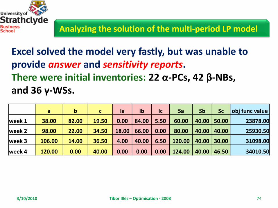
Analyzing the solution of the multi-period LP model

Excel solved the model very fastly, but was unable to provide answer and sensitivity reports.There were initial inventories: 22 α-PCs, 42 β-NBs, and 36 γ-WSs.

a b c Ia Ib Ic Sa Sb Sc obj func value

week 1 38.00 82.00 19.50 0.00 84.00 5.50 60.00 40.00 50.00 23878.00

week 2 98.00 22.00 34.50 18.00 66.00 0.00 80.00 40.00 40.00 25930.50

week 3 106.00 14.00 36.50 4.00 40.00 6.50 120.00 40.00 30.00 31098.00

week 4 120.00 0.00 40.00 0.00 0.00 0.00 124.00 40.00 46.50 34010.50


Analyzing the solution of the multi-period LP model

2000 ≤ 2000

120 ≤ 120

19.5 ≤ 48

2000 ≤ 2000120 ≤ 120

34.5 ≤ 482000 ≤ 2000

120 ≤ 12036.5 ≤ 48

2000 ≤ 2000

120 ≤ 12040 ≤ 48

22 equal 2242 equal 4236 equal 36

-5.7E-14 equal 02.63E-13 equal 0

7.53E-13 equal 01.42E-14 equal 0

-5.9E-13 equal 0

7.82E-14 equal 0

3.69E-13 equal 02.13E-14 equal 0-3.1E-13 equal 0

622 equal 6224.37E-11 equal 0

-5.8E-11 equal 0

-7.3E-12 equal 0

20 ≤ 60 ≤ 60

20 ≤ 40 ≤ 40

20 ≤ 50 ≤ 50

20 ≤ 80 ≤ 80

20 ≤ 40 ≤ 40

20 ≤ 40 ≤ 40

20 ≤ 120 ≤ 120

20 ≤ 40 ≤ 40

20 ≤ 30 ≤ 30

20 ≤ 124 ≤ 140

20 ≤ 40 ≤ 40

20 ≤ 46.5 ≤ 70Production constraints

Flow and balance equations

Bounds


Multi-period linear programming problem: sparsity

single period model multi-period model

# of variables 3 40

# of constraints 3 52

# of non-zeros 6 118

# of zeros 3 1862

sparsity 66.66% 0.057%

Large scale and multiperiod models are sparse models. Sparsity value of large scale models are usually below 2%.

lectures 3 & 4: linear programming problem formulation

Documents