lectures on coupling - university of warwick · aim and style of lectures these lectures aim to...
TRANSCRIPT

Lectures on CouplingEPSRC/RSS GTP course, September 2005
Wilfrid [email protected]
Department of Statistics, University of Warwick
12th–16th September 2005

Lectures
Introduction
Coupling and Monotonicity
Representation
Approximation using coupling
Mixing of Markov chains
The Coupling Zoo
Perfection (CFTP I)
Perfection (CFTP II)
Perfection (FMMR)
Sundry further topics in CFTP
Conclusion

Monday 12 September09.00–09.05 Welcome09.05–10.00 Coupling 1 Introduction10.00–11.00 Bayes 111.00–11.30 Coffee/Tea11.30–12.30 Bayes 212.30–13.45 Lunch13.45–14.45 Coupling 2 Monotonicity14.45–15.45 Coupling 3 Representation15.45–16.15 Coffee/Tea16.15–17.15 Bayes 319.00–21.00 Dinner
Tuesday 13 September09.00–10.00 Bayes 410.00–11.00 Bayes Practical 111.00–11.30 Coffee/Tea11.30–12.30 Coupling 4 Approximation12.30–13.45 Lunch13.45–14.45 Coupling 5 Mixing14.45–15.45 Coupling practical A0.0215.45–16.15 Coffee/Tea16.15–17.15 Bayes 519.00–21.00 Dinner
(all lectures in MS.04)
Wednesday 14 September09.00–10.00 Coupling 6 The Zoo10.00–11.00 Coupling 7 Perfection: CFTP (I)11.00–11.30 Coffee/Tea11.30–12.30 Bayes Exercises12.30–13.45 Lunch13.45–18.00 Excursion19.00–21.00 Dinner
Thursday 15 September09.00–10.00 Bayes 610.00–11.00 Bayes 711.00–11.30 Coffee/Tea11.30–12.30 Coupling practical A0.0212.30–13.45 Lunch13.45–14.45 Coupling 8 Perfection: CFTP (II)14.45–15.45 Coupling 9 Perfection: FMMR15.45–16.15 Coffee/Tea16.15–17.15 Bayes 819.00–21.00 Dinner (Sutherland Suite)
Friday 16 September09.00–10.00 Coupling 10 Sundry topics10.00–11.00 Bayes Practical 2 (MS.04/A1.01)11.00–11.30 Coffee/Tea11.30–13.00 Bayes Practical 2 (MS.04/A1.01)13.00 Lunch/departure

Lecture 1: Introduction
“The best thing for being sad,” replied Merlin, beginning to puff and blow,“is to learn something. That’s the only thing that never fails. You may growold and trembling in your anatomies, you may lie awake at night listening tothe disorder of your veins, you may miss your only love, you may see theworld about you devastated by evil lunatics, or know your honour trampledin the sewers of baser minds. There is only one thing for it then – to learn.Learn why the world wags and what wags it. That is the only thing whichthe mind can never exhaust, never alienate, never be tortured by, neverfear or distrust, and never dream of regretting. Learning is the only thingfor you. Look what a lot of things there are to learn.”
— T. H. White, “The Once and Future King”
IntroductionA brief description of couplingAim and style of lecturesReading and browsingSoundbitesCard shufflingHistorical example

A brief description of coupling
“Coupling” is a many-valued term in mathematical science!
In a probabilist’s vocabulary it means: finding out about arandom system X by constructing a second randomsystem Y on the same probability space (maybeaugmented by a seasoning of extra randomness).
Careful construction, choosing the right system Y ,designing the right kind of dependence between X and Y ,leads to clear intuitive explanations of important factsabout X .

Aim and style of lectures
These lectures aim to survey ideas from coupling theory,using a pattern of beginning with an intuitive example,developing the idea of the example, and then remarking onfurther ramifications of the theory.
Aiming for style of Rubeus Hagrid’s “Care of Magical Creatures”rather than Dolores Umbridge’s “Defence against the Dark Arts”.
Carelessly planned projects take three times longer tocomplete than expected. Carefully planned projectstake four times longer to complete than expected,mostly because the planners expect their planning toreduce the time it takes.

Aim and style of lectures
These lectures aim to survey ideas from coupling theory,using a pattern of beginning with an intuitive example,developing the idea of the example, and then remarking onfurther ramifications of the theory.Aiming for style of Rubeus Hagrid’s “Care of Magical Creatures”rather than Dolores Umbridge’s “Defence against the Dark Arts”.
Carelessly planned projects take three times longer tocomplete than expected. Carefully planned projectstake four times longer to complete than expected,mostly because the planners expect their planning toreduce the time it takes.

Reading and browsingBooks and URIs
I History: Doeblin (1938), see also Lindvall (1991).
I Literature: Breiman (1992), Lindvall (2002), Pollard (2001),Thorisson (2000), Aldous and Fill (200x);
I http://www.warwick.ac.uk/go/wsk/talks/gtp.pdf
http://research.microsoft.com/ ∼dbwilson/exact/
Of making many books there is no end,and much study wearies the body.
— Ecclesiastics 12:12b

Reading and browsingBooks and URIs
I History: Doeblin (1938), see also Lindvall (1991).I Literature: Breiman (1992), Lindvall (2002), Pollard (2001),
Thorisson (2000), Aldous and Fill (200x);
I http://www.warwick.ac.uk/go/wsk/talks/gtp.pdf
http://research.microsoft.com/ ∼dbwilson/exact/
Of making many books there is no end,and much study wearies the body.
— Ecclesiastics 12:12b

Soundbites
Probability theory has a right and a left hand— Breiman (1992, Preface).
Coupling: more a probabilistic sub-culturethan an identifiable theory.
A proof using coupling is rather like a well-told joke: ifit has to be explained then it loses much of its force.
Coupling arguments are like counting arguments— but without natural numbers.
Coupling is the soul of probability.

Card shufflingTop card shuffle
Draw: Top card moved to random location in pack.Q: How long to equilibrium?
A: Two alternative strategies:
(a) wait till bottom card gets to top, then draw one more;
(b) or wait till next-to-bottom card gets to top, then draw onemore.
I HINT: consider the various possible orders of the cardslying below the specified card at each stage.
I Note existence of special states, such that you should stopafter moving from such a state (unusual in general!).
I Mean time till equilibrium is order n log(n).

Card shufflingTop card shuffle
Draw: Top card moved to random location in pack.Q: How long to equilibrium?A: Two alternative strategies:
(a) wait till bottom card gets to top, then draw one more;
(b) or wait till next-to-bottom card gets to top, then draw onemore.
I HINT: consider the various possible orders of the cardslying below the specified card at each stage.
I Note existence of special states, such that you should stopafter moving from such a state (unusual in general!).
I Mean time till equilibrium is order n log(n).
EXERCISE 1.1

Card shufflingRiffle shuffle
Draw: split card pack into two parts using Binomial distribution.Recombine uniformly at random.Q: How long to equilibrium (uniform randomness)?
I DEVIOUS HINT: Apply a time reversal and re-labelling, soreversed process looks like this: to each card assign asequence of random bits (0, 1). Remove cards with top bitset, move to top of pack, remove top bits, repeat . . . .
I How long till resulting random permutation is uniform?Depends on how long sequence must be in order to labeleach card uniquely.
I Time-reversals will be important later when discussingqueues, dominated CFTP , and Siegmund duality.
EXERCISE 1.2

Historical exampleFirst appearance of coupling
Treatment of convergence of Markov chains to statisticalequilibrium by Doeblin (1938).
Theorem 1.1 (Doeblin coupling)For a finite state space Markov chain, consider two copies; onestarted in equilibrium (P [X = j] = πj ), one at some specifiedstarting state. Run the chains independently till they meet, orcouple. Then:
12
∑j
∣∣∣πj − p(n)ij
∣∣∣ ≤ P [ no coupling by time n] (1)
We develop the theory for this later, when we discuss thecoupling inequality.
EXERCISE 1.3 EXERCISE 1.4 EXERCISE 1.5

Historical exampleSuccessful coupling
Definition 1.2We say a coupling between two random processes X and Ysucceeds if almost surely X and Y eventually meet.
The Doeblin coupling succeeds for all finite aperiodicirreducible Markov chains (via the lemma which says thereis T ≥ 0 such that p(n)
ij > 0 once n ≥ N), and indeed for allcountable positive-recurrent aperiodic Markov chains.
Successful couplings control rate of convergence toequilibrium.
Thorisson has constructed a coupling proof that p(n)ij → 0
for countable null-recurrent Markov chains.

Lecture 2: Coupling and Monotonicity
MONOTONOUS
ADJECTIVE: Arousing no interest or curiosity: boring,drear, dreary, dry, dull, humdrum, irksome, stuffy, tedious,tiresome, uninteresting, weariful, wearisome, weary. SeeEXCITE.
— Roget’s II: The New Thesaurus, Third Edition. 1995
Coupling and MonotonicityBinomial monotonicityRabbitsFKG inequalityFortuin-Kasteleyn representation

Binomial monotonicity
The simplest examples of monotonicity arise for Binomialrandom variables, thought of as sums of Bernoulli randomvariables.
I Suppose X is distributed as Binomial(n, p). Show thatP [X ≥ k ] is an increasing function of the successprobability p.
EXERCISE 2.1
I Generalize to show uniqueness of critical probability forpercolation on a Euclidean lattice.
EXERCISE 2.2

Increasing events
Here is the notion which makes these examples work.
Definition 2.1Consider a sequence of (binary) random variables Y1, Y2, . . . ,Yn. An increasing event A for this sequence is determined bythe values Y1 = y1, Y2 = y2, . . . , Yn = yn, and the indicator I [A]is an increasing function of the y1, y2, . . . , yn.
Both [X ≥ k ] and “there is an infinite connected component”are increasing events. The idea is developed further in thediscussion of the FKG inequality below.

Continuous Rabbits
Kendall and Saunders (1983) used coupling to analyzecompeting myxomatosis epidemics in Australian rabbits.
s′ = −α1β1si1 − α2β2si2
i ′1 = α1β1si1 − β1i1 ,
r ′1 = β1i1i ′2 = α2β2si2 − β2i2 , r ′2 = β2i2
(2)
Suppose α1 > α2.
Susceptibles s;
Infectives i1,
i2; Removals r1, r2.
Are r1(∞), r2(∞) appropriately monotonic in i1, i2?

Continuous Rabbits
Kendall and Saunders (1983) used coupling to analyzecompeting myxomatosis epidemics in Australian rabbits.
s′ = −α1β1si1 − α2β2si2
i ′1 = α1β1si1 − β1i1 ,
r ′1 = β1i1
i ′2 = α2β2si2 − β2i2 ,
r ′2 = β2i2
(2)
Suppose α1 > α2.
Susceptibles s;
Infectives i1, i2;
Removals r1, r2.
Are r1(∞), r2(∞) appropriately monotonic in i1, i2?

Continuous Rabbits
Kendall and Saunders (1983) used coupling to analyzecompeting myxomatosis epidemics in Australian rabbits.
s′ = −α1β1si1 − α2β2si2i ′1 = α1β1si1 − β1i1 ,
r ′1 = β1i1
i ′2 = α2β2si2 − β2i2 ,
r ′2 = β2i2
(2)
Suppose α1 > α2.
Susceptibles s; Infectives i1, i2;
Removals r1, r2.
Are r1(∞), r2(∞) appropriately monotonic in i1, i2?
Continuous Rabbits
Kendall and Saunders (1983) used coupling to analyzecompeting myxomatosis epidemics in Australian rabbits.
s′ = −α1β1si1 − α2β2si2i ′1 = α1β1si1 − β1i1 , r ′1 = β1i1i ′2 = α2β2si2 − β2i2 , r ′2 = β2i2 (2)
Suppose α1 > α2.
Susceptibles s; Infectives i1, i2; Removals r1, r2.
Are r1(∞), r2(∞) appropriately monotonic in i1, i2?

Continuous Rabbits
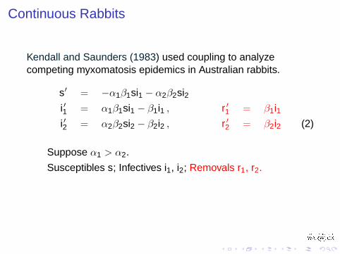
Kendall and Saunders (1983) used coupling to analyzecompeting myxomatosis epidemics in Australian rabbits.
s′ = −α1β1si1 − α2β2si2i ′1 = α1β1si1 − β1i1 , r ′1 = β1i1i ′2 = α2β2si2 − β2i2 , r ′2 = β2i2 (2)
Suppose α1 > α2.
Susceptibles s; Infectives i1, i2; Removals r1, r2.
Are r1(∞), r2(∞) appropriately monotonic in i1, i2?

Stochastic Rabbits
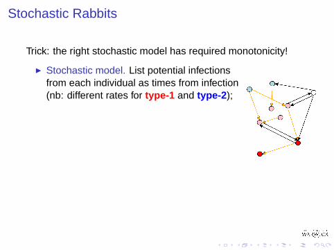
Trick: the right stochastic model has required monotonicity!
I Stochastic model. List potential infectionsfrom each individual as times from infection(nb: different rates for type-1 and type-2 );
I Converting type-1 initial infective tosusceptible or to type-2 infective “clearly”delays type-1 epidemic: hence desiredmonotonicity for stochastic model.
I Deterministic model inherits monotonicity.
Just one out of many applications to epidemic theory: see also Balland Donnelly (1995). For coupling in spatial epidemics, see Mollison(1977), Haggstrom and Pemantle (1998, 2000).

Stochastic Rabbits
Trick: the right stochastic model has required monotonicity!
I Stochastic model. List potential infectionsfrom each individual as times from infection(nb: different rates for type-1 and type-2 );
I Converting type-1 initial infective tosusceptible or to type-2 infective “clearly”delays type-1 epidemic: hence desiredmonotonicity for stochastic model.
I Deterministic model inherits monotonicity.
Just one out of many applications to epidemic theory: see also Balland Donnelly (1995). For coupling in spatial epidemics, see Mollison(1977), Haggstrom and Pemantle (1998, 2000).

Stochastic Rabbits
Trick: the right stochastic model has required monotonicity!
I Stochastic model. List potential infectionsfrom each individual as times from infection(nb: different rates for type-1 and type-2 );
I Converting type-1 initial infective tosusceptible or to type-2 infective “clearly”delays type-1 epidemic: hence desiredmonotonicity for stochastic model.
I Deterministic model inherits monotonicity.
Just one out of many applications to epidemic theory: see also Balland Donnelly (1995). For coupling in spatial epidemics, see Mollison(1977), Haggstrom and Pemantle (1998, 2000). EXERCISE 2.3
FKG inequality
Theorem 2.2 (FKG for independent Bernoulli set-up)Suppose A, B are two increasing events for binary Y1, Y2, . . . ,Yn: then they are positively correlated;
P [A ∩ B] ≥ P [A] P [B] . (3)
The FKG inequality generalizes:I replace sets A, B by “increasing random variables”
(Grimmett 1999, §2.2);I allow Y1, Y2, . . . , Yn to “interact attractively” (Preston 1977,
or vary as described in the Exercise!).EXERCISE 2.4

Fortuin-Kasteleyn representation
Site-percolation can be varied to produce bond-percolation: fora given graph G suppose the edges or bonds are independentlyopen or not to the flow of a fluid with probability p.The probability of any given configuration is
p#(open bonds) × (1− p)#(closed bonds) . (4)
Suppose we want a new dependent bond-percolation model,biased towards the formation of many different connectedcomponents or clusters in the resulting random graph.
Definition 2.3 (Random Cluster model)The probability of any given configuration is proportional to
q#(components) × p#(open bonds) × (1− p)#(closed bonds) . (5)

Fortuin-Kastelyn representation (ctd.)
Suppose q = 2 and we assign signs ±1 independently to eachof the resulting clusters. This produces a random configurationassigning Si = ±1 to each site i (according to which clustercontains it): a spin model. Remarkably:
Theorem 2.4 (Fortuin-Kasteleyn representation)The spin model described above is the Ising model on G: theprobability of any given configuration is proportional to
exp
12β
∑i∼j
SiSj
∝ exp (β ×#(similar pairs)) (6)
where p = 1− e−β .
We have coupled the Ising model (of statistical mechanics andimage analysis fame) to a dependent bond-percolation model!
EXERCISE 2.5

Comparison
Moreover, we can compare probabilities of increasing eventsfor bond-percolation and random cluster models:
Theorem 2.5 (Fortuin-Kasteleyn comparison)Suppose A is an increasing event for bond-percolation. Then
P [A under bond percolation(p)] ≤≤ P
[A under random cluster(p′, q)
]≤
≤ P[A under bond percolation(p′)
]when q ≥ 1 and p/(1− p) = p′/(q(1− p′)).
The FKG inequality holds for the general random cluster modelwhen q ≥ 1.

“The good Christian should beware of mathematiciansand all those who make empty prophecies. Thedanger already exists that mathematicians have madea covenant with the devil to darken the spirit andconfine man in the bonds of Hell.”
— St. Augustine

Lecture 3: Representation
Wrights’ Axioms of Queuing Theory.
1. If you have a choice between waiting here and waiting there, waitthere.
2. All things being equal, it is better to wait at the front of the line.3. There is no point in waiting at the end of the line.
But note Wrights’ Paradox:4. If you don’t wait at the end of the line, you’ll never get to the front.5. Whichever line you are in, the others always move faster.
— Charles R. B. Wright
RepresentationQueuesStrassen’s resultPrincesses and FrogsAge brings avariceCapitalist geographyBack to probabilitySplit chains and small sets

Queues
We have already seen how coupling can provide importantrepresentations: the Fortuin-Kastelyn representation for theIsing model. Here is another representation, from the theory ofqueues, which also introduces ideas of time reversal which willbe important later.
Recall the standard notation for queues: an M/M/1 queue hasMarkov inputs (arrivals according to Poisson process), Markovservice times (Exponential, which counts as Markov bymemoryless property), and 1 server.When we move away from Markov then analysis gets harder: ifinputs are GI (General Input, but independent) or if servicetimes are General (but still independent) then we can useembedding methods to reduce to discrete time Markov chaintheory. If both (GI/G/1, independent service and inter-arrivaltimes) then even this is not available!

Queues
We have already seen how coupling can provide importantrepresentations: the Fortuin-Kastelyn representation for theIsing model. Here is another representation, from the theory ofqueues, which also introduces ideas of time reversal which willbe important later.Recall the standard notation for queues: an M/M/1 queue hasMarkov inputs (arrivals according to Poisson process), Markovservice times (Exponential, which counts as Markov bymemoryless property), and 1 server.
When we move away from Markov then analysis gets harder: ifinputs are GI (General Input, but independent) or if servicetimes are General (but still independent) then we can useembedding methods to reduce to discrete time Markov chaintheory. If both (GI/G/1, independent service and inter-arrivaltimes) then even this is not available!

Queues
We have already seen how coupling can provide importantrepresentations: the Fortuin-Kastelyn representation for theIsing model. Here is another representation, from the theory ofqueues, which also introduces ideas of time reversal which willbe important later.Recall the standard notation for queues: an M/M/1 queue hasMarkov inputs (arrivals according to Poisson process), Markovservice times (Exponential, which counts as Markov bymemoryless property), and 1 server.When we move away from Markov then analysis gets harder: ifinputs are GI (General Input, but independent) or if servicetimes are General (but still independent) then we can useembedding methods to reduce to discrete time Markov chaintheory. If both (GI/G/1, independent service and inter-arrivaltimes) then even this is not available!

Lindley’s representation I
However Lindley noticed a beautiful representation for waitingtime Wn of customer n in terms of services Sn and interarrivalsXn . . .
Theorem 3.1 (Lindley’s equation)Consider the GI/G/1 queue waiting time identity.
Wn+1 = max{0, Wn + Sn − Xn+1} = max{0, Wn + ηn}= max{0, ηn, ηn + ηn−1, . . . , ηn + ηn−1 + . . . + η1}=D max{0, η1, η1 + η2, . . . , η1 + η2 + . . . + ηn}
and thus we obtain the steady-state expression
W∞ =D max{0, η1, η1 + η2, . . .} . (7)
If Var [ηi ] < ∞ then SLLN/CLT/random walk theory shows W∞will be finite if and only if E [ηi ] < 0 or ηi ≡ 0.

Lindley’s representation II
Coupling enters in at the crucial time-reversal step!
This idea will reappear later in our discussion of thefalling-leaves model . . . .
Supposing we lose independence? Loynes (1962)discovered a coupling application to queues with (forexample) general dependent stationary inputs andassociated service times, pre-figuring CFTP .
EXERCISE 3.1 EXERCISE 3.2

Queues and coupling
Theorem 3.2Suppose queue arrivals follow a stationary point processstretching back to time −∞. Denote arrivals/associated servicetimes in (s, t ] by Ns,t (stationarity: statistics of process{Ns,s+u : u ≥ 0} do not depend on s). Let QT denote thebehaviour of the queue observed from time 0 onwards if begunwith 0 customers at time −T . The queue converges tostatistical equilibrium if and only if
limT→∞
QT exists almost surely.
Stoyan (1983) develops this kind of idea. Kendall (1983) givesan application to storage problems.
EXERCISE 3.3

Strassen’s result
When can we closely couple 1 two random variables? Thisquestion is easy to deal with in one dimension, using theinverse probability transform, taken up below. However there isalso a beautiful treatment of Strassen’s treatment of themultivariate case, based on the Marriage Lemma and due toDudley (1976). Here is a fairy-tale explanation, building onPollard (2001)’s charming exposition.
1Relates to the Prohorov metric.

Princesses and Frogs
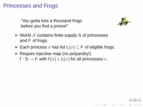
“You gotta kiss a thousand frogsbefore you find a prince!”
I World X contains finite supply S of princessesand F of frogs.
I Each princess σ has list L(σ) ⊆ F of eligible frogs.I Require injective map (no polyandry!)
f : S → F with f (σ) ∈ L(σ) for all princesses σ.
Lemma 3.3 (Marriage Lemma)A suitable injection f : S → F exists exactly whenfor all sets of princesses A ⊆ S
#A ≤ #L(A) for L(A) =⋃{L(σ) : σ ∈ A} . (8)

Princesses and Frogs
“You gotta kiss a thousand frogsbefore you find a prince!”
I World X contains finite supply S of princessesand F of frogs.
I Each princess σ has list L(σ) ⊆ F of eligible frogs.
I Require injective map (no polyandry!)f : S → F with f (σ) ∈ L(σ) for all princesses σ.
Lemma 3.3 (Marriage Lemma)A suitable injection f : S → F exists exactly whenfor all sets of princesses A ⊆ S
#A ≤ #L(A) for L(A) =⋃{L(σ) : σ ∈ A} . (8)
Princesses and Frogs
“You gotta kiss a thousand frogsbefore you find a prince!”
I World X contains finite supply S of princessesand F of frogs.
I Each princess σ has list L(σ) ⊆ F of eligible frogs.I Require injective map (no polyandry!)
f : S → F with f (σ) ∈ L(σ) for all princesses σ.
Lemma 3.3 (Marriage Lemma)A suitable injection f : S → F exists exactly whenfor all sets of princesses A ⊆ S
#A ≤ #L(A) for L(A) =⋃{L(σ) : σ ∈ A} . (8)

Princesses and Frogs
“You gotta kiss a thousand frogsbefore you find a prince!”
I World X contains finite supply S of princessesand F of frogs.
I Each princess σ has list L(σ) ⊆ F of eligible frogs.I Require injective map (no polyandry!)
f : S → F with f (σ) ∈ L(σ) for all princesses σ.
Lemma 3.3 (Marriage Lemma)A suitable injection f : S → F exists exactly whenfor all sets of princesses A ⊆ S
#A ≤ #L(A) for L(A) =⋃{L(σ) : σ ∈ A} . (8)

If Equation (8) fails then there are not enough frogs to go roundsome set A!On the other hand Equation (8) suffices for just one princess(#S = 1).So use induction on #S ≥ 1:
I Princess σ1 imperiously chooses first frog f1(σ1) on her listL(σ1). Remaining princesses S \ {σ1} check franticallywhether reduced lists L(σ) \ {f1(σ1)} will work(they use Equation (8) and induction ).
I If not, (8) fails for some ∅ 6= A ⊂ S \ {σ1}, using thereduced lists:
#L(A) \ {f1(σ1)} < #A
which forces #L(A) = #A (use original Equation (8)).I A set A of aggrieved princesses splits off with their
preferred frogs L(A). The aggrieved set can solve theirmarriage problem (use Equation (8), induction ).

If Equation (8) fails then there are not enough frogs to go roundsome set A!On the other hand Equation (8) suffices for just one princess(#S = 1).So use induction on #S ≥ 1:
I Princess σ1 imperiously chooses first frog f1(σ1) on her listL(σ1). Remaining princesses S \ {σ1} check franticallywhether reduced lists L(σ) \ {f1(σ1)} will work(they use Equation (8) and induction ).
I If not, (8) fails for some ∅ 6= A ⊂ S \ {σ1}, using thereduced lists:
#L(A) \ {f1(σ1)} < #A
which forces #L(A) = #A (use original Equation (8)).
I A set A of aggrieved princesses splits off with theirpreferred frogs L(A). The aggrieved set can solve theirmarriage problem (use Equation (8), induction ).

If Equation (8) fails then there are not enough frogs to go roundsome set A!On the other hand Equation (8) suffices for just one princess(#S = 1).So use induction on #S ≥ 1:
I Princess σ1 imperiously chooses first frog f1(σ1) on her listL(σ1). Remaining princesses S \ {σ1} check franticallywhether reduced lists L(σ) \ {f1(σ1)} will work(they use Equation (8) and induction ).
I If not, (8) fails for some ∅ 6= A ⊂ S \ {σ1}, using thereduced lists:
#L(A) \ {f1(σ1)} < #A
which forces #L(A) = #A (use original Equation (8)).I A set A of aggrieved princesses splits off with their
preferred frogs L(A). The aggrieved set can solve theirmarriage problem (use Equation (8), induction ).

I What of remainder S \ A with residual listsL(σ) = L(σ) \ L(A)? Observe:
#(L(B) ∪ L(A)) = #L(B) + #L(A)
= #L(B ∪ A)
≥ #(B ∪ A) = #B + #A = #B + #L(A) .
I So Equation (8) holds for remainder with residual lists:the proof can now be completed by induction .
“If you eat a live frog in the morning,nothing worse will happen to either ofyou for the rest of the day.”

Age brings avarice
“Kissing don’t last, cooking gold do”
The princesses, now happily married to their frogs, grow older.Inevitably they begin to exhibit mercenary tendencies — a sadbut frequent tendency amongst royalty. Their major interest isnow in gold .
I World X contains finite set G of goldmines g of capacityµ(g) tons per year respectively.
I Each princess σ ∈ S requires ν(σ) tons of gold per yearfrom her list K (σ) ⊆ G of appropriate goldmines.
I Require gold assignment using probability kernel
p : S → P(G) ,
p(σ, ·) supported by K (σ), with∑
σ ν(σ)p(σ, g) ≤ µ(g).

Lemma 3.4 (Marriage Lemma version 2)
A suitable probability kernel p(σ, g) exists exactly when for allsets A ⊆ S of princesses
ν(A) ≤ µ(K (A)) for K (A) =⋃{K (σ) : σ ∈ A} . (9)
Proof.Princesses aren’t interested in small change and fractions oftons of gold. So we approximate by assuming µ(g), ν(σ) arenon-negative integers. (Can then proceed to rationals, then toreals!)Now de-personalize those avaricious princesses: apply theMarriage Lemma to tons of gold instead of princesses!
“For the love of money is a root of all kinds of evil”— Paul of Tarsus, 1 Timothy 6:10 (NIV)

Lemma 3.4 (Marriage Lemma version 2)
A suitable probability kernel p(σ, g) exists exactly when for allsets A ⊆ S of princesses
ν(A) ≤ µ(K (A)) for K (A) =⋃{K (σ) : σ ∈ A} . (9)
Proof.Princesses aren’t interested in small change and fractions oftons of gold. So we approximate by assuming µ(g), ν(σ) arenon-negative integers. (Can then proceed to rationals, then toreals!)
Now de-personalize those avaricious princesses: apply theMarriage Lemma to tons of gold instead of princesses!
“For the love of money is a root of all kinds of evil”— Paul of Tarsus, 1 Timothy 6:10 (NIV)

Lemma 3.4 (Marriage Lemma version 2)
A suitable probability kernel p(σ, g) exists exactly when for allsets A ⊆ S of princesses
ν(A) ≤ µ(K (A)) for K (A) =⋃{K (σ) : σ ∈ A} . (9)
Proof.Princesses aren’t interested in small change and fractions oftons of gold. So we approximate by assuming µ(g), ν(σ) arenon-negative integers. (Can then proceed to rationals, then toreals!)Now de-personalize those avaricious princesses: apply theMarriage Lemma to tons of gold instead of princesses!
“For the love of money is a root of all kinds of evil”— Paul of Tarsus, 1 Timothy 6:10 (NIV)

Lemma 3.4 (Marriage Lemma version 2)
A suitable probability kernel p(σ, g) exists exactly when for allsets A ⊆ S of princesses
ν(A) ≤ µ(K (A)) for K (A) =⋃{K (σ) : σ ∈ A} . (9)
Proof.Princesses aren’t interested in small change and fractions oftons of gold. So we approximate by assuming µ(g), ν(σ) arenon-negative integers. (Can then proceed to rationals, then toreals!)Now de-personalize those avaricious princesses: apply theMarriage Lemma to tons of gold instead of princesses!
“For the love of money is a root of all kinds of evil”— Paul of Tarsus, 1 Timothy 6:10 (NIV)

Capitalist geography
The princesses’ preferences for goldmines are geographicallybased. Suppose princess σ is located at x(σ) ∈ X , andgoldmine g at y(g) ∈ X . Then
L(σ) = {g ∈ G : dist(x(σ), y(g)) < ε} for fixed ε > 0 .
Avoid quarrels: assume x(σ) are distinct and also y(g) aredistinct.
The king has been watching all these arrangements withinterest. To make domestic life easier, he arranges for aconvenient orbiting space-station to hold a modest amount ofgold (ε′ tons, topped up each year). The princesses agree toadd the space-station to their lists.

Capitalist geography
The princesses’ preferences for goldmines are geographicallybased. Suppose princess σ is located at x(σ) ∈ X , andgoldmine g at y(g) ∈ X . Then
L(σ) = {g ∈ G : dist(x(σ), y(g)) < ε} for fixed ε > 0 .
Avoid quarrels: assume x(σ) are distinct and also y(g) aredistinct.The king has been watching all these arrangements withinterest. To make domestic life easier, he arranges for aconvenient orbiting space-station to hold a modest amount ofgold (ε′ tons, topped up each year). The princesses agree toadd the space-station to their lists.

The second form of the Marriage Lemma shows, the royaldemand for gold can be met so long as∑
σ:x(σ)∈B
ν(σ) ≤∑
g:dist(g,σ)<ε for x(σ)∈B
µ(g) + ε′ .
for any subset B ⊆ X .(nb: L({σ : x(σ) ∈ B}) = {g : dist(g, σ) < ε for x(σ) ∈ B}).

Back to probability
Replace princesses, gold demands, and locations by aX -valued random variable X , distribution P.Similarly replace goldmines, annual yields, and locations by aprobability distribution Q. When is close-coupling possible?
Theorem 3.5 (Strassen’s Theorem)For probability distributions P, Q on X , we can find X -valuedrandom variables X, Y with distributions P, Q and such that
P [dist(X , Y ) > ε] ≤ ε′ (10)
exactly when, for all subsets B ⊆ X ,
P[B] ≤ Q[x : dist(x , B) < ε] + ε′ . (11)

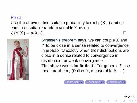
Proof.Use the above to find suitable probability kernel p(X , ·) and soconstruct suitable random variable Y usingL (Y |X ) = p(X , ·),
Strassen’s theorem says, we can couple X andY to be close in a sense related to convergencein probability exactly when their distributions areclose in a sense related to convergence indistribution, or weak convergence.The above works for finite X . For general X usemeasure-theory (Polish X , measurable B . . . ).
EXERCISE 3.4 EXERCISE 3.5 EXERCISE 3.6

Split chains and small sets I
Strassen’s theorem is useful when we want close-coupling (withjust a small probability of being far away!). Suppose we wantsomething different: a coupling with a positive chance of beingexactly equal and otherwise no constraint. (Related to notion ofconvergence stationnaire, or “parking convergence”, forstochastic process theory.) Given two overlapping probabilitydensities f and g, we implement the coupling (X , Y ) as follows:
I Compute α =∫
(f ∧ g)(x) d x , and with probability α returna draw of X = Y from the density (f ∧ g)/α.
I Otherwise draw X from (f − f ∧ g)/(1− α) and Y from(g − f ∧ g)/(1− α).
This is related to the method of rejection sampling in stochasticsimulation.
EXERCISE 3.7

Split chains and small sets II
From Doeblin’s time onwards, probabilists have applied this tostudy Markov chain transition probability kernels:
Definition 3.6 (Small set condition)Let X be a Markov chain on a state space S, transition kernelp(x , d y). The set C ⊆ S is a small set of order k if for someprobability measure ν and some α > 0
p(k)(x , d y) ≥ I [C] (x)× α ν(d y) . (12)

Split chains and small sets III
It is a central result that small sets (possibly of arbitrarily highorder) exist for any modestly regular Markov chain (proof ineither of Nummelin 1984; Meyn and Tweedie 1993).
Theorem 3.7Let X be a Markov chain on a non-discrete state space S,transition kernel p(x , d y). Suppose an (order 1) small setC ⊆ S exists. The dynamics of X can be represented using anew Markov chain on S ∪ {c}, for c a regenerativepseudo-state.
For a more sophisticated theorem see Nummelin (1978), alsoAthreya and Ney (1978).
DISPLAY

Small sets
Higher-order small sets (p(x , d y) → p(k)(x , d y)) systematicallyreduce general state space theory to discrete. See Meyn andTweedie (1993) also Roberts and Rosenthal (2001).
Small sets of order 1 need not exist:
but will if (a) the kernel p(x , d y) has a density and (b) chain issub-sampled at even times.

Small sets
Higher-order small sets (p(x , d y) → p(k)(x , d y)) systematicallyreduce general state space theory to discrete. See Meyn andTweedie (1993) also Roberts and Rosenthal (2001).
Small sets of order 1 need not exist:
but will if
(a) the kernel p(x , d y) has a density and (b) chain issub-sampled at even times.

Small sets
Higher-order small sets (p(x , d y) → p(k)(x , d y)) systematicallyreduce general state space theory to discrete. See Meyn andTweedie (1993) also Roberts and Rosenthal (2001).
Small sets of order 1 need not exist:
but will if (a) the kernel p(x , d y) has a density. . .
and (b) chainis sub-sampled at even times.

Small sets
Higher-order small sets (p(x , d y) → p(k)(x , d y)) systematicallyreduce general state space theory to discrete. See Meyn andTweedie (1993) also Roberts and Rosenthal (2001).
Small sets of order 1 need not exist:
but will if (a) the kernel p(x , d y) has a density and (b) chain issub-sampled at even times.

Small sets and discretization of Markov chains
Theorem 3.8 (Kendall and Montana 2002)If the Markov chain has a measurable transition density p(x , y)then the two-step density p(2)(x , y) can be expressed(non-uniquely) as a non-negative countable sum
p(2)(x , y) =∑
i
fi(x)gi(y) . (13)
So an evenly sampled Markov chain with transition density is alatent discrete Markov chain, with transition probabilities
pij =
∫gi(u)fj(u) d u . (14)
DISPLAY

Lecture 4: Approximation using coupling
Five is a sufficiently close approximation to infinity.— Robert Firth
Approximation using couplingSkorokhod representation for weak convergenceCentral Limit Theorem and Brownian embeddingStein-Chen method for Poisson approximation

Skorokhod representation for weak convergence
We recall the inverse probability transform, and its use forsimulation of random variables.
Definition 4.1 (inverse probability transform)If
F : R → [0, 1]
is increasing and right-continuous (ie: a distribution function)then we define its inverse as follows:
F−1(u) = inf{t : F (t) ≥ u} . (15)
A graph of a distribution function helps to explain the reason forthis definition!
DISPLAY

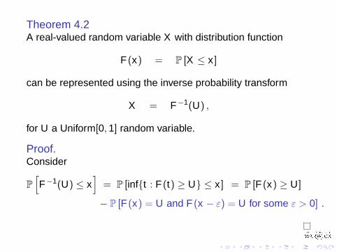
Theorem 4.2A real-valued random variable X with distribution function
F (x) = P [X ≤ x ]
can be represented using the inverse probability transform
X = F−1(U) ,
for U a Uniform[0, 1] random variable.
Proof.Consider
P[F−1(U) ≤ x
]= P [inf{t : F (t) ≥ U} ≤ x ]
= P [F (x) ≥ U] − . . .

Theorem 4.2A real-valued random variable X with distribution function
F (x) = P [X ≤ x ]
can be represented using the inverse probability transform
X = F−1(U) ,
for U a Uniform[0, 1] random variable.
Proof.Consider
P[F−1(U) ≤ x
]= P [inf{t : F (t) ≥ U} ≤ x ]
= P [F (x) ≥ U] − . . .

Theorem 4.2A real-valued random variable X with distribution function
F (x) = P [X ≤ x ]
can be represented using the inverse probability transform
X = F−1(U) ,
for U a Uniform[0, 1] random variable.
Proof.Consider
P[F−1(U) ≤ x
]= P [inf{t : F (t) ≥ U} ≤ x ] = P [F (x) ≥ U] − . . .
Theorem 4.2A real-valued random variable X with distribution function
F (x) = P [X ≤ x ]
can be represented using the inverse probability transform
X = F−1(U) ,
for U a Uniform[0, 1] random variable.
Proof.Consider
P[F−1(U) ≤ x
]= P [inf{t : F (t) ≥ U} ≤ x ] = P [F (x) ≥ U]
− . . .
− P [F (x) = U and F (x − ε) = U for some ε > 0] .

Theorem 4.2A real-valued random variable X with distribution function
F (x) = P [X ≤ x ]
can be represented using the inverse probability transform
X = F−1(U) ,
for U a Uniform[0, 1] random variable.
Proof.Consider
P[F−1(U) ≤ x
]= P [inf{t : F (t) ≥ U} ≤ x ] = P [F (x) ≥ U]
− . . .
= F (x) .

If we do this with a single U for an entire weaklyconvergent sequence of random variables, thus couplingthe sequence, then we convert weak convergence toalmost sure convergence.
For more general multivariate random variables (eg: withvalues in Polish spaces) we refer back to the methods ofStrassen’s theorem.
EXERCISE 4.1 EXERCISE 4.2

Central Limit Theorem and Brownian embedding
Theorem 4.3A zero-mean random variable X of finite variance can berepresented as X = B(T ) for a stopping time T of finite mean.Thus Strong Law of Large Numbers and Brownian scalingimply CLT!
Use the following basic facts about Brownian motion:I Strong Markov property;I Continuous sample paths;I Martingale property: E [B(S)] = 0 if S is a “bounded”
stopping time (B|[0,S) bounded will do!);
I moreover, in that case E[B(S)2
]= E [S];
I Scaling: B(N·)/√
N has the same distribution as B(·).

Central Limit Theorem and Brownian embedding
Theorem 4.3A zero-mean random variable X of finite variance can berepresented as X = B(T ) for a stopping time T of finite mean.Thus Strong Law of Large Numbers and Brownian scalingimply CLT!
Use the following basic facts about Brownian motion:
I Strong Markov property;I Continuous sample paths;I Martingale property: E [B(S)] = 0 if S is a “bounded”
stopping time (B|[0,S) bounded will do!);
I moreover, in that case E[B(S)2
]= E [S];
I Scaling: B(N·)/√
N has the same distribution as B(·).

Central Limit Theorem and Brownian embedding
Theorem 4.3A zero-mean random variable X of finite variance can berepresented as X = B(T ) for a stopping time T of finite mean.Thus Strong Law of Large Numbers and Brownian scalingimply CLT!
Use the following basic facts about Brownian motion:I Strong Markov property;
I Continuous sample paths;I Martingale property: E [B(S)] = 0 if S is a “bounded”
stopping time (B|[0,S) bounded will do!);
I moreover, in that case E[B(S)2
]= E [S];
I Scaling: B(N·)/√
N has the same distribution as B(·).

Central Limit Theorem and Brownian embedding
Theorem 4.3A zero-mean random variable X of finite variance can berepresented as X = B(T ) for a stopping time T of finite mean.Thus Strong Law of Large Numbers and Brownian scalingimply CLT!
Use the following basic facts about Brownian motion:I Strong Markov property;I Continuous sample paths;
I Martingale property: E [B(S)] = 0 if S is a “bounded”stopping time (B|[0,S) bounded will do!);
I moreover, in that case E[B(S)2
]= E [S];
I Scaling: B(N·)/√
N has the same distribution as B(·).

Central Limit Theorem and Brownian embedding
Theorem 4.3A zero-mean random variable X of finite variance can berepresented as X = B(T ) for a stopping time T of finite mean.Thus Strong Law of Large Numbers and Brownian scalingimply CLT!
Use the following basic facts about Brownian motion:I Strong Markov property;I Continuous sample paths;I Martingale property: E [B(S)] = 0 if S is a “bounded”
stopping time (B|[0,S) bounded will do!);
I moreover, in that case E[B(S)2
]= E [S];
I Scaling: B(N·)/√
N has the same distribution as B(·).

Central Limit Theorem and Brownian embedding
Theorem 4.3A zero-mean random variable X of finite variance can berepresented as X = B(T ) for a stopping time T of finite mean.Thus Strong Law of Large Numbers and Brownian scalingimply CLT!
Use the following basic facts about Brownian motion:I Strong Markov property;I Continuous sample paths;I Martingale property: E [B(S)] = 0 if S is a “bounded”
stopping time (B|[0,S) bounded will do!);
I moreover, in that case E[B(S)2
]= E [S];
I Scaling: B(N·)/√
N has the same distribution as B(·).
EXERCISE 4.3

The promised proof of the CLT runs as follows:
Xn = B(σ1 + . . . + σn)− B(σ1 + . . . + σn−1)
σ1 + . . . + σN
N E [σ]→ 1 almost surely by SLLN
(now convert construction to use a scaled path,
and exploit continuity of the path)
B(σ
(N)1 + . . . + σ
(N)N
N E [σ]) → B(1) almost surely
and B(1) is Gaussian . . .
LHS ∼ 1√N E [σ]
B(σ1 + . . . + σN) =1√
N E [σ]
N∑1
Xn .
We deduce the following convergence in distribution:
1√N E [σ]
N∑1
Xn → B(1) .

This gives excellent intuition into extensions such as theLindeberg condition: clearly the CLT should still work aslong as σ
(N)1 + . . . + σ
(N)n /N converges to a non-random
constant (essentially a matter for SLLN for non-negativerandom variables!).
We don’t even require independence: some kind ofmartingale conditions should (and do!) suffice.
But most significantly this approach suggests how toformulate a Functional CLT: the random-walk evolution X1,X2, . . . should converge as random walk path to Brownianmotion. An example of this kind of result is given in Kendalland Westcott (1987).

Stein-Chen method for Poisson approximation
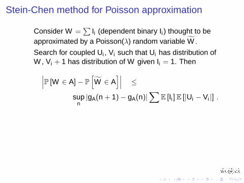
Consider W =∑
Ii (dependent binary Ii ) thought to beapproximated by a Poisson(λ) random variable W .
Search for coupled Ui , Vi such that Ui has distribution ofW , Vi + 1 has distribution of W given Ii = 1.
Then∣∣∣P [W ∈ A]− P[W ∈ A
]∣∣∣ ≤
supn|gA(n + 1)− gA(n)|
∑E [Ii ] E [|Ui − Vi |] .
Here gA(n) satisfies the Stein Estimating Equation
λgA(n + 1) = ngA(n) + I [n ∈ A]− P[W ∈ A
]. (16)

Stein-Chen method for Poisson approximation
Consider W =∑
Ii (dependent binary Ii ) thought to beapproximated by a Poisson(λ) random variable W .
Search for coupled Ui , Vi such that Ui has distribution ofW , Vi + 1 has distribution of W given Ii = 1.
Then∣∣∣P [W ∈ A]− P[W ∈ A
]∣∣∣ ≤
supn|gA(n + 1)− gA(n)|
∑E [Ii ] E [|Ui − Vi |] .
Here gA(n) satisfies the Stein Estimating Equation
λgA(n + 1) = ngA(n) + I [n ∈ A]− P[W ∈ A
]. (16)
Stein-Chen method for Poisson approximation
Consider W =∑
Ii (dependent binary Ii ) thought to beapproximated by a Poisson(λ) random variable W .
Search for coupled Ui , Vi such that Ui has distribution ofW , Vi + 1 has distribution of W given Ii = 1. Then∣∣∣P [W ∈ A]− P
[W ∈ A
]∣∣∣ ≤
supn|gA(n + 1)− gA(n)|
∑E [Ii ] E [|Ui − Vi |] .
Here gA(n) satisfies the Stein Estimating Equation
λgA(n + 1) = ngA(n) + I [n ∈ A]− P[W ∈ A
]. (16)
EXERCISE 4.4 EXERCISE 4.5 EXERCISE 4.6 EXERCISE 4.7 EXERCISE 4.8

Consider∣∣∣P [W ∈ A]− P[W ∈ A
]∣∣∣ ≤
supn|gA(n + 1)− gA(n)|
∑E [Ii ] E [|Ui − Vi |] .
After analysis (see Barbour, Holst, and Janson 1992)
supn|gA(n)| ≤ min
{1,
1√λ
}(17)
supn|gA(n + 1)− gA(n)| ≤ 1− e−λ
λ≤ min
{1,
1λ
}(18)
Even better, if Ui ≥ Vi (say), the sum collapses:∑E [Ii ] E [|Ui − Vi |] = λ− Var [W ] . (19)

“There are only 10 types of people in this world:those who understand binary and those who don’t.”

Lecture 5: Mixing of Markov chains
What is (15 minus three times five) plus
I (20 minus four times five) plusI (36 minus nine times four) plusI (72 minus nine times eight) plusI (98 minus eight times twelve) plusI (54 minus seven times eight)?
A lot of work for nothing.
http://cnonline.net/ ∼TheCookieJar/
Mixing of Markov chainsCoupling inequalityVery simple mixing exampleSlice samplerStrong stationary times

Lecture 5: Mixing of Markov chains
What is (15 minus three times five) plusI (20 minus four times five) plus
I (36 minus nine times four) plusI (72 minus nine times eight) plusI (98 minus eight times twelve) plusI (54 minus seven times eight)?
A lot of work for nothing.
http://cnonline.net/ ∼TheCookieJar/
Mixing of Markov chainsCoupling inequalityVery simple mixing exampleSlice samplerStrong stationary times

Lecture 5: Mixing of Markov chains
What is (15 minus three times five) plusI (20 minus four times five) plusI (36 minus nine times four) plus
I (72 minus nine times eight) plusI (98 minus eight times twelve) plusI (54 minus seven times eight)?
A lot of work for nothing.
http://cnonline.net/ ∼TheCookieJar/
Mixing of Markov chainsCoupling inequalityVery simple mixing exampleSlice samplerStrong stationary times

Lecture 5: Mixing of Markov chains
What is (15 minus three times five) plusI (20 minus four times five) plusI (36 minus nine times four) plusI (72 minus nine times eight) plus
I (98 minus eight times twelve) plusI (54 minus seven times eight)?
A lot of work for nothing.
http://cnonline.net/ ∼TheCookieJar/
Mixing of Markov chainsCoupling inequalityVery simple mixing exampleSlice samplerStrong stationary times

Lecture 5: Mixing of Markov chains
What is (15 minus three times five) plusI (20 minus four times five) plusI (36 minus nine times four) plusI (72 minus nine times eight) plusI (98 minus eight times twelve) plus
I (54 minus seven times eight)?
A lot of work for nothing.
http://cnonline.net/ ∼TheCookieJar/
Mixing of Markov chainsCoupling inequalityVery simple mixing exampleSlice samplerStrong stationary times

Lecture 5: Mixing of Markov chains
What is (15 minus three times five) plusI (20 minus four times five) plusI (36 minus nine times four) plusI (72 minus nine times eight) plusI (98 minus eight times twelve) plusI (54 minus seven times eight)?
A lot of work for nothing.
http://cnonline.net/ ∼TheCookieJar/
Mixing of Markov chainsCoupling inequalityVery simple mixing exampleSlice samplerStrong stationary times

Coupling inequality
Suppose X is a Markov chain, with equilibrium distribution π,for which we can produce a coupling between any two points x ,y , which succeeds at time Tx ,y < ∞. Then
disttv (L (Xn) , π) ≤ maxy{P
[Tx ,y > t
]} . (20)
Useful bounds depend on finding and analyzing the rightcoupling!Optimal couplings (inequality becomes equality, at price ingeneral of being non-co-adaptive): Griffeath (1975), Pitman(1976), Goldstein (1979).The coupling inequality is also the basis for an empiricalapproach to convergence estimation (Johnson 1996).

Coupling inequality
Suppose X is a Markov chain, with equilibrium distribution π,for which we can produce a coupling between any two points x ,y , which succeeds at time Tx ,y < ∞. Then
disttv (L (Xn) , π) ≤ maxy{P
[Tx ,y > t
]} . (20)
Useful bounds depend on finding and analyzing the rightcoupling!
Optimal couplings (inequality becomes equality, at price ingeneral of being non-co-adaptive): Griffeath (1975), Pitman(1976), Goldstein (1979).The coupling inequality is also the basis for an empiricalapproach to convergence estimation (Johnson 1996).

Coupling inequality
Suppose X is a Markov chain, with equilibrium distribution π,for which we can produce a coupling between any two points x ,y , which succeeds at time Tx ,y < ∞. Then
disttv (L (Xn) , π) ≤ maxy{P
[Tx ,y > t
]} . (20)
Useful bounds depend on finding and analyzing the rightcoupling!Optimal couplings (inequality becomes equality, at price ingeneral of being non-co-adaptive): Griffeath (1975), Pitman(1976), Goldstein (1979).
The coupling inequality is also the basis for an empiricalapproach to convergence estimation (Johnson 1996).

Coupling inequality
Suppose X is a Markov chain, with equilibrium distribution π,for which we can produce a coupling between any two points x ,y , which succeeds at time Tx ,y < ∞. Then
disttv (L (Xn) , π) ≤ maxy{P
[Tx ,y > t
]} . (20)
Useful bounds depend on finding and analyzing the rightcoupling!Optimal couplings (inequality becomes equality, at price ingeneral of being non-co-adaptive): Griffeath (1975), Pitman(1976), Goldstein (1979).The coupling inequality is also the basis for an empiricalapproach to convergence estimation (Johnson 1996).
EXERCISE 5.1

Very simple mixing example
Utterly the simplest case: a Markov chain on {0, 1}.
Let X , Y start at 0, 1, with transitionsI 0 → 1 at rate 1/α,
I and 1 → 0 at rate 1/α.
DISPLAY
Supply (a) Poisson process (rate 1/α) of 0 → 1 transitions,(b) ditto of 1 → 0 transitions. Apply them where applicableto X , Y . Clearly X , Y have desired distributions.
Coupling happens at first instant of combined Poissonprocess, hence at Exponential(2/α) random time.
The coupled equilibrium chain begins in between X and Y ,and is equal to both at time of coupling. Hence we canestimate rate of convergence to equilibrium . . .
EXERCISE 5.2

Slice sampler
Task is to draw from density f (x). Here is a one-dimensionalexample! (But note, this is only interesting because it can bemade to work in many dimensions . . . ) Suppose f unimodal.Define g0(y), g1(y) implicitly by: [g0(y), g1(y)] is thesuperlevel set {x : f (x) ≥ y}. Alternate between drawing yuniformly from [0, f (x)] and drawing x uniformly from[g0(y), g1(y)].
DISPLAY
Roberts and Rosenthal (1999, Theorem 12) show rapidconvergence (order of 530 iterations!) under a specific variationof log-concavity.
EXERCISE 5.3

Strong stationary times I
Definition 5.1 (Aldous and Diaconis 1987; Diaconis andFill 1990)The random stopping time T is a strong stationary time for theMarkov chain X (whose equilibrium distribution is π) if
P [T = k , Xk = s] = πs × P [T = k ] . (21)

Strong stationary times II
Application to shuffling pack of n cards by randomtranspositions (Broder): based on notion of checked cards.
Transpose by choosing 2 cards at random; LH, RH.Check card pointed to by LH if
either LH, RH are the same unchecked card;or LH is unchecked, RH is checked.
I Inductive claim: given number of checked cards, positionsin pack of checked cards, list of values of cards, then thethe map of checked card to value is uniformly random.
Let Tm be time when m cards checked. Then (induction)T =
∑n−1m=0 Tm is a strong stationary time.
EXERCISE 5.4

Strong stationary times II
Application to shuffling pack of n cards by randomtranspositions (Broder): based on notion of checked cards.
Transpose by choosing 2 cards at random; LH, RH.
Check card pointed to by LH if
either LH, RH are the same unchecked card;or LH is unchecked, RH is checked.
I Inductive claim: given number of checked cards, positionsin pack of checked cards, list of values of cards, then thethe map of checked card to value is uniformly random.
Let Tm be time when m cards checked. Then (induction)T =
∑n−1m=0 Tm is a strong stationary time.
EXERCISE 5.4

Strong stationary times II
Application to shuffling pack of n cards by randomtranspositions (Broder): based on notion of checked cards.
Transpose by choosing 2 cards at random; LH, RH.Check card pointed to by LH if
either LH, RH are the same unchecked card;or LH is unchecked, RH is checked.
I Inductive claim: given number of checked cards, positionsin pack of checked cards, list of values of cards, then thethe map of checked card to value is uniformly random.
Let Tm be time when m cards checked. Then (induction)T =
∑n−1m=0 Tm is a strong stationary time.
EXERCISE 5.4

Strong stationary times II
Application to shuffling pack of n cards by randomtranspositions (Broder): based on notion of checked cards.
Transpose by choosing 2 cards at random; LH, RH.Check card pointed to by LH if
either LH, RH are the same unchecked card;
or LH is unchecked, RH is checked.
I Inductive claim: given number of checked cards, positionsin pack of checked cards, list of values of cards, then thethe map of checked card to value is uniformly random.
Let Tm be time when m cards checked. Then (induction)T =
∑n−1m=0 Tm is a strong stationary time.
EXERCISE 5.4

Strong stationary times II
Application to shuffling pack of n cards by randomtranspositions (Broder): based on notion of checked cards.
Transpose by choosing 2 cards at random; LH, RH.Check card pointed to by LH if
either LH, RH are the same unchecked card;or LH is unchecked, RH is checked.
I Inductive claim: given number of checked cards, positionsin pack of checked cards, list of values of cards, then thethe map of checked card to value is uniformly random.
Let Tm be time when m cards checked. Then (induction)T =
∑n−1m=0 Tm is a strong stationary time.
EXERCISE 5.4

Strong stationary times II
Application to shuffling pack of n cards by randomtranspositions (Broder): based on notion of checked cards.
Transpose by choosing 2 cards at random; LH, RH.Check card pointed to by LH if
either LH, RH are the same unchecked card;or LH is unchecked, RH is checked.
I Inductive claim: given number of checked cards, positionsin pack of checked cards, list of values of cards, then thethe map of checked card to value is uniformly random.
Let Tm be time when m cards checked. Then (induction)T =
∑n−1m=0 Tm is a strong stationary time.
EXERCISE 5.4

Strong stationary times III
We know Tm+1 − Tm is Geometrically distributed with successprobability (n −m)(m + 1)/n2.
So mean of T is
E
[n−1∑m=0
Tm
]=
n−1∑m=0
n2
n + 1
(1
n −m+
1m + 1
)≈ 2n log n .
MOREOVER: T =∑n−1
m=0 Tm is a discrete version of time tocomplete infection for simple epidemic (without recovery) in nindividuals, starting with 1 infective, individuals contacting atrate n2. A classic calculation tells us T/(2n log n) has a limitingdistribution.NOTE: by group representation theory (or a more carefulprobabilistic construction) the correct asymptotic is 1
2n log n.
EXERCISE 5.5

Strong stationary times III
We know Tm+1 − Tm is Geometrically distributed with successprobability (n −m)(m + 1)/n2. So mean of T is
E
[n−1∑m=0
Tm
]=
n−1∑m=0
n2
n + 1
(1
n −m+
1m + 1
)≈ 2n log n .
MOREOVER: T =∑n−1
m=0 Tm is a discrete version of time tocomplete infection for simple epidemic (without recovery) in nindividuals, starting with 1 infective, individuals contacting atrate n2. A classic calculation tells us T/(2n log n) has a limitingdistribution.
NOTE: by group representation theory (or a more carefulprobabilistic construction) the correct asymptotic is 1
2n log n.
EXERCISE 5.5

Strong stationary times III
We know Tm+1 − Tm is Geometrically distributed with successprobability (n −m)(m + 1)/n2. So mean of T is
E
[n−1∑m=0
Tm
]=
n−1∑m=0
n2
n + 1
(1
n −m+
1m + 1
)≈ 2n log n .
MOREOVER: T =∑n−1
m=0 Tm is a discrete version of time tocomplete infection for simple epidemic (without recovery) in nindividuals, starting with 1 infective, individuals contacting atrate n2. A classic calculation tells us T/(2n log n) has a limitingdistribution.NOTE: by group representation theory (or a more carefulprobabilistic construction) the correct asymptotic is 1
2n log n.
EXERCISE 5.5

They told me you had proven itAbout a month before.
The proof was valid, more or lessBut rather less than more.
He sent them word that we would tryTo pass where they had failed
And after we were done, to themThe new proof would be mailed.
My notion was to start againIgnoring all they’d done
We quickly turned it into codeTo see if it would run.
When they discovered our resultsTheir blood began to freeze
Instead of understanding itWe’d run thirteen MCMC’s .
Don’t tell a soul about all thisFor it must ever be
A secret, kept from all the restBetween yourself and me.

Lecture 6: The Coupling Zoo
There is a whole variety of different ways of constructingcouplings. Here is a zoo containing some representativespecimens.
But my Totem saw the shame; from his ridgepole shrine he came,And he told me in a vision of the night:“There are nine and sixty ways of constructing tribal lays,And every single one of them is right!”
In the Neolithic Age — Rudyard Kipling
The Coupling ZooZoo taxonomy

The Coupling ZooA politically inspired taxonomy
Coupling method: Before coupling happens . . .Independent (Doeblin) Be independent.
Synchronous Do the same.Reflection Do the opposite.Ornstein (random walks) Be a liberal democrat: agree big steps,
otherwise be independent . . .Mineka (random walks) . . . be new labour: difference is
simple symmetric random walk.Vasershtein Maximize immediate success.Time-changed Run chains at varying rates.Maximal (non-adaptive) Practice inside-trading.
(Griffeath 1975; Goldstein 1979)Shift Do the same thing at different times!
(Aldous and Thorisson 1993)
The easiest coupling method to study!
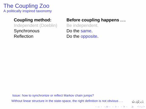
The Coupling ZooA politically inspired taxonomy
Coupling method: Before coupling happens . . .Independent (Doeblin) Be independent.Synchronous Do the same.Reflection Do the opposite.
Ornstein (random walks) Be a liberal democrat: agree big steps,otherwise be independent . . .
Mineka (random walks) . . . be new labour: difference issimple symmetric random walk.
Vasershtein Maximize immediate success.Time-changed Run chains at varying rates.Maximal (non-adaptive) Practice inside-trading.
(Griffeath 1975; Goldstein 1979)Shift Do the same thing at different times!
(Aldous and Thorisson 1993)
Issue: how to synchronize or reflect Markov chain jumps?
Without linear structure in the state-space, the right definition is not obvious . . .

The Coupling ZooA politically inspired taxonomy
Coupling method: Before coupling happens . . .Independent (Doeblin) Be independent.Synchronous Do the same.Reflection Do the opposite.Ornstein (random walks) Be a liberal democrat: agree big steps,
otherwise be independent . . .
Mineka (random walks) . . . be new labour: difference issimple symmetric random walk.
Vasershtein Maximize immediate success.Time-changed Run chains at varying rates.Maximal (non-adaptive) Practice inside-trading.
(Griffeath 1975; Goldstein 1979)Shift Do the same thing at different times!
(Aldous and Thorisson 1993)
Great advantage: converts random walks to
random walks with symmetric bounded increments!
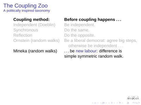
The Coupling ZooA politically inspired taxonomy
Coupling method: Before coupling happens . . .Independent (Doeblin) Be independent.Synchronous Do the same.Reflection Do the opposite.Ornstein (random walks) Be a liberal democrat: agree big steps,
otherwise be independent . . .Mineka (random walks) . . . be new labour: difference is
simple symmetric random walk.
Vasershtein Maximize immediate success.Time-changed Run chains at varying rates.Maximal (non-adaptive) Practice inside-trading.
(Griffeath 1975; Goldstein 1979)Shift Do the same thing at different times!
(Aldous and Thorisson 1993)

The Coupling ZooA politically inspired taxonomy
Coupling method: Before coupling happens . . .Independent (Doeblin) Be independent.Synchronous Do the same.Reflection Do the opposite.Ornstein (random walks) Be a liberal democrat: agree big steps,
otherwise be independent . . .Mineka (random walks) . . . be new labour: difference is
simple symmetric random walk.Vasershtein Maximize immediate success.
Time-changed Run chains at varying rates.Maximal (non-adaptive) Practice inside-trading.
(Griffeath 1975; Goldstein 1979)Shift Do the same thing at different times!
(Aldous and Thorisson 1993)
The Vasershtein coupling is related to small-set coupling:
look at the overlap between jump distributions.

The Coupling ZooA politically inspired taxonomy
Coupling method: Before coupling happens . . .Independent (Doeblin) Be independent.Synchronous Do the same.Reflection Do the opposite.Ornstein (random walks) Be a liberal democrat: agree big steps,
otherwise be independent . . .Mineka (random walks) . . . be new labour: difference is
simple symmetric random walk.Vasershtein Maximize immediate success.Time-changed Run chains at varying rates.
Maximal (non-adaptive) Practice inside-trading.(Griffeath 1975; Goldstein 1979)
Shift Do the same thing at different times!(Aldous and Thorisson 1993)
Vary time-rates to make sure coupling happens
before either of the processes hits a fixed boundary (Kendall 1994).

The Coupling ZooA politically inspired taxonomy
Coupling method: Before coupling happens . . .Independent (Doeblin) Be independent.Synchronous Do the same.Reflection Do the opposite.Ornstein (random walks) Be a liberal democrat: agree big steps,
otherwise be independent . . .Mineka (random walks) . . . be new labour: difference is
simple symmetric random walk.Vasershtein Maximize immediate success.Time-changed Run chains at varying rates.Maximal (non-adaptive) Practice inside-trading.
(Griffeath 1975; Goldstein 1979)
Shift Do the same thing at different times!(Aldous and Thorisson 1993)
Suppose we allow non-adaptive coupling strategies (one process depends
on future of other!). This relates to bounded space-time harmonic functions.

The Coupling ZooA politically inspired taxonomy
Coupling method: Before coupling happens . . .Independent (Doeblin) Be independent.Synchronous Do the same.Reflection Do the opposite.Ornstein (random walks) Be a liberal democrat: agree big steps,
otherwise be independent . . .Mineka (random walks) . . . be new labour: difference is
simple symmetric random walk.Vasershtein Maximize immediate success.Time-changed Run chains at varying rates.Maximal (non-adaptive) Practice inside-trading.
(Griffeath 1975; Goldstein 1979)Shift Do the same thing at different times!
(Aldous and Thorisson 1993)Shift-coupling requires simply that processes X , Y should agree after
different stopping times S, T . Related to bounded harmonic functions.

The Coupling ZooA politically inspired taxonomy
Coupling method: Before coupling happens . . .Independent (Doeblin) Be independent.Synchronous Do the same.Reflection Do the opposite.Ornstein (random walks) Be a liberal democrat: agree big steps,
otherwise be independent . . .Mineka (random walks) . . . be new labour: difference is
simple symmetric random walk.Vasershtein Maximize immediate success.Time-changed Run chains at varying rates.Maximal (non-adaptive) Practice inside-trading.
(Griffeath 1975; Goldstein 1979)Shift Do the same thing at different times!
(Aldous and Thorisson 1993)

The Coupling ZooA conclusion
So which coupling is the best?It all depends what you want to do . . .
What did the Colonel’s Lady think?Nobody never knew.Somebody asked the Sergeant’s Wife,An’ she told ’em true!When you get to a man in the case,They’re like as a row of pins –For the Colonel’s Lady an’ Judy O’GradyAre sisters under their skins!
The Ladies — Rudyard Kipling, Barrack Room Ballads
EXERCISE 6.1 EXERCISE 6.2 EXERCISE 6.3

Lecture 7: Perfection (CFTP I)
“You can arrive (mayan arivan on-when) for any sittingyou like without prior (late fore-when) reservationbecause you can book retrospectively, as it were whenyou return to your own time. (you can have on-bookhaventa forewhen presooning returningwentaretrohome.)”
Douglas Adams — Hitchhiker’s Guide to the Galaxy
Perfection (CFTP I)Back to mixingClassic CFTPCFTP theoremFalling leavesIsing model CFTPSmall-set CFTP
EXERCISE 7.1 EXERCISE 7.2 EXERCISE 7.3 EXERCISE 7.4 EXERCISE 7.5

The constructive nature of probabilistic coupling (“to build Yusing the randomness of X ”) makes it close in spirit to the taskof constructing good stochastic simulations. Recently the linkbetween coupling and simulation has been strengthened instriking ways, resulting in so-called “exact” or “perfectsimulation”.
Haggstrom (2002) includes discussion ofsome of these ideas at the level of astudent monograph.
See alsoI Aldous and Fill (200x);I Møller and Waagepetersen (2003);
and
http://research.microsoft.com/ ∼dbwilson/exact/

More on mixing
Recall (continuous-time!) random walk on {0, 1}.
Construction: Supply (a) Poisson process (rate 1/α) of0 → 1 transitions, (b) ditto of 1 → 0 transitions. Apply themwhere applicable to X started at 0, Y started at 1. DISPLAY
Clearly X , Y have desired distributions.
Questions:
Does it make sense to return first coupled value? (Yeshere, no in “nearly every” other case.)
But suppose I run algorithm from [−T , 0] for increasing T ,instead of from [0, T ] for increasing T ? (This will workalways: this is CFTP .)
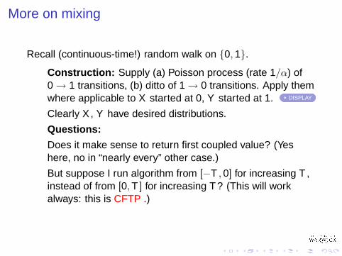

Classic CFTP
Conventionally, the Markov chain is extended into thefuture T using innovations.
Equilibrium in the unreachably far infinite future T →∞.
Ergodic theorists have always known of an alternative:
view the chain as produced at time t = 0 by innovationsacting from some starting point −T in the past:
flows not processes, dependence on initial conditions,X0 at 0 no longer Markov as −T → −∞,
if the value of X0 stabilizes to a single value then thisvalue is a draw from equilibrium!
DISPLAY

Classic CFTP
Conventionally, the Markov chain is extended into thefuture T using innovations.
Equilibrium in the unreachably far infinite future T →∞.
Ergodic theorists have always known of an alternative:
view the chain as produced at time t = 0 by innovationsacting from some starting point −T in the past:
flows not processes, dependence on initial conditions,X0 at 0 no longer Markov as −T → −∞, BUT . . .
if the value of X0 stabilizes to a single value then thisvalue is a draw from equilibrium!
DISPLAY

Classic CFTP
Conventionally, the Markov chain is extended into thefuture T using innovations.
Equilibrium in the unreachably far infinite future T →∞.
Ergodic theorists have always known of an alternative:
view the chain as produced at time t = 0 by innovationsacting from some starting point −T in the past:
flows not processes, dependence on initial conditions,X0 at 0 no longer Markov as −T → −∞, but:
if the value of X0 stabilizes to a single value then thisvalue is a draw from equilibrium!
DISPLAY

Theorem 7.1If coalescence is almost sure then CFTP delivers a samplefrom the equilibrium distribution of the Markov chain Xcorresponding to the random input-output maps F(−u,v ].
Proof.For each [−n,∞) use input-output maps F(−n,t]. Assume finitecoalescence time −n = −T for F(−n,0]. Then
X−nt = F(−n,t](0) for − n ≤ t .
X−n0 = X−T
0 whenever − n ≤ −T ;
L(X−n
0
)= L
(X 0
n
).
If X converges to an equilibrium π then
disttv (L(
X−T0
), π) = lim
ndisttv (L
(X−n
0
), π) = lim
ndisttv (L
(X 0
n
), π) = 0 .

Theorem 7.1If coalescence is almost sure then CFTP delivers a samplefrom the equilibrium distribution of the Markov chain Xcorresponding to the random input-output maps F(−u,v ].
Proof.For each [−n,∞) use input-output maps F(−n,t]. Assume finitecoalescence time −n = −T for F(−n,0].
Then
X−nt = F(−n,t](0) for − n ≤ t .
X−n0 = X−T
0 whenever − n ≤ −T ;
L(X−n
0
)= L
(X 0
n
).
If X converges to an equilibrium π then
disttv (L(
X−T0
), π) = lim
ndisttv (L
(X−n
0
), π) = lim
ndisttv (L
(X 0
n
), π) = 0 .

Theorem 7.1If coalescence is almost sure then CFTP delivers a samplefrom the equilibrium distribution of the Markov chain Xcorresponding to the random input-output maps F(−u,v ].
Proof.For each [−n,∞) use input-output maps F(−n,t]. Assume finitecoalescence time −n = −T for F(−n,0]. Then
X−nt = F(−n,t](0) for − n ≤ t .
X−n0 = X−T
0 whenever − n ≤ −T ;
L(X−n
0
)= L
(X 0
n
).
If X converges to an equilibrium π then
disttv (L(
X−T0
), π) = lim
ndisttv (L
(X−n
0
), π) = lim
ndisttv (L
(X 0
n
), π) = 0 .

Theorem 7.1If coalescence is almost sure then CFTP delivers a samplefrom the equilibrium distribution of the Markov chain Xcorresponding to the random input-output maps F(−u,v ].
Proof.For each [−n,∞) use input-output maps F(−n,t]. Assume finitecoalescence time −n = −T for F(−n,0]. Then
X−nt = F(−n,t](0) for − n ≤ t .
X−n0 = X−T
0 whenever − n ≤ −T ;
L(X−n
0
)= L
(X 0
n
).
If X converges to an equilibrium π then
disttv (L(
X−T0
), π) = lim
ndisttv (L
(X−n
0
), π) = lim
ndisttv (L
(X 0
n
), π) = 0 .

Falling leaves
Kendall and Thonnes (1999) describe a visual and geometricapplication of CFTP in mathematical geology: this particularexample being well-known to workers in the field previous tothe introduction of CFTP itself.
Occlusion CFTP for the falling leaves ofFontainbleau.
(Why “occlusion”? David Wilson’s terminol-ogy: this CFTP algorithm builds up the resultpiece-by-piece with no back-tracking.) DISPLAY
EXERCISE 7.6

Falling leaves
Kendall and Thonnes (1999) describe a visual and geometricapplication of CFTP in mathematical geology: this particularexample being well-known to workers in the field previous tothe introduction of CFTP itself.
Occlusion CFTP for the falling leaves ofFontainbleau.
(Why “occlusion”? David Wilson’s terminol-ogy: this CFTP algorithm builds up the resultpiece-by-piece with no back-tracking.)
DISPLAY
EXERCISE 7.6

Falling leaves
Kendall and Thonnes (1999) describe a visual and geometricapplication of CFTP in mathematical geology: this particularexample being well-known to workers in the field previous tothe introduction of CFTP itself.
Occlusion CFTP for the falling leaves ofFontainbleau.
(Why “occlusion”? David Wilson’s terminol-ogy: this CFTP algorithm builds up the resultpiece-by-piece with no back-tracking.) DISPLAY
EXERCISE 7.6

Ising model (I)
The original Propp and Wilson (1996) idea showed how tomake exact draws from the critical Ising model. A rathersimpler application uses the heat-bath sampler to makeexact draws from the sub-critical Ising model.
Classic CFTP for the Ising model (sim-ple, sub-critical case). Heat-bath dy-namics run from past; compare resultsfrom maximal and minimal starting con-ditions. DISPLAY

Ising model (II)
Approaches based on Swendsen-Wang ideas work forcritical case (Huber 2003).
On the other hand, conditioning by noisy data convenientlyreduces the difficulties caused by phase-transitionphenomena.
Classic CFTP for the Ising model condi-tioned by noisy data. Without influencefrom data (“external magnetic field”) thisIsing model would be super-critical.
DISPLAY

Small-set CFTP
A common misconception is that CFTP requires an orderedstate-space. Green and Murdoch (1999) showed how to usesmall sets to carry out CFTP when the state-space iscontinuous with no helpful ordering. Their prescription includesthe use of a partition by several small sets, to speed upcoalescence.Small set CFTP in nearly the simplestpossible case: a triangular kernel over [0, 1].
DISPLAY

“What’s past is –”“– is very much in the present. Brigadier, you neverdid understand the interrelation of time.”
— The Brigadier and the Doctor, in “MawdrynUndead”

Lecture 8: Perfection (CFTP II)
- “I think there may be one or two steps in your logic thatI have failed to grasp, Mister Stibbons,” said theArchchancellor coldly. “I suppose you’re not intendingto shoot your own grandfather, by any chance?”
- “Of course not!” snapped Ponder, “I don’t even knowwhat he looked like. He died before I was born.”
- “Ah-hah !”The faculty members of Unseen University discuss timetravel
— The Last Continent, Terry Pratchett
Perfection (CFTP II)Point patternsDominated CFTP for area-interaction point processesFast attractive area-interaction CFTPLayered Multishift CFTPPerpetuities
Dominated CFTP
Successful application of CFTP usually requires thecombination of a number of tricks. We have already seenexamples in which monotonicity plays a part, either openly(random walk, Ising) or concealed (dead leaves).
One of the major issues concerns how to deal with Markovchains that are not “bounded” (technically speaking, notuniformly ergodic, in sense of Defn. 10.2).2
Consider the point-pattern-valued birth-death processesoften used in modelling spatial point processes . . .
2“uniformly ergodic”: rate of convergenceto equilibrium doesn’t depend on starting point.

Point processes
Algorithm to generate a random point pattern X (see, eg,Stoyan et al. 1995). Repeat the following:
I suppose the current value of X is X = x :
I after Exponential (#(x) +∫
W λ∗(x ; ξ) d ξ) random time
I Death: with probability #(x)/(#(x) +∫
W λ∗(x ; ξ) d ξ),choose a point η of x at random and delete it from x ;
I Birth: otherwise generate a new point ξ with probabilitydensity proportional to λ∗(x ; ξ), and add it to x .
An easy coupling argument shows this chain is geometricallyergodic3 (in sense of Defn. 10.3) for sensible λ∗(x ; ξ)!
Note the significant role of Papangelou conditional intensityλ∗(x ; ξ) (“chance of a point at x given rest of pattern ξ”).
3“geometrically ergodic”: achievesequilibrium geometrically fast.
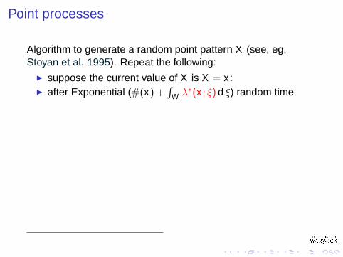
Point processes
Algorithm to generate a random point pattern X (see, eg,Stoyan et al. 1995). Repeat the following:
I suppose the current value of X is X = x :I after Exponential (#(x) +
∫W λ∗(x ; ξ) d ξ) random time
I Death: with probability #(x)/(#(x) +∫
W λ∗(x ; ξ) d ξ),choose a point η of x at random and delete it from x ;
I Birth: otherwise generate a new point ξ with probabilitydensity proportional to λ∗(x ; ξ), and add it to x .
An easy coupling argument shows this chain is geometricallyergodic3 (in sense of Defn. 10.3) for sensible λ∗(x ; ξ)!
Note the significant role of Papangelou conditional intensityλ∗(x ; ξ) (“chance of a point at x given rest of pattern ξ”).
3“geometrically ergodic”: achievesequilibrium geometrically fast.

Examples
Strauss process
λ∗(x ; ξ) = γneighbours of x within distance r (22)
yields density weighting realizations using
γpairs in pattern at distance r or less .
Area-interaction process
λ∗(x ; ξ) = γ−area of region within r of x but not rest of pattern
density ∝ γ−area of region within distance r of pattern (23)
DISPLAY

Domination by a random process
Dominated CFTP replaces the deterministic maximum by aknown random process run backwards in time, providing startsfor upper- and lower-envelope processes guaranteed tosandwich a valid simulation.

Nonlinear birth and death processes
Suppose X is a nonlinear immigration-death process:
X → X − 1 at rate µX ;X → X + 1 . . . αX where αX ≤ α∞.
No maximum (not uniformly ergodic); no classic CFTP!
We can bound by a linear immigration-death process Y :
Y → Y − 1 at rate µY ;Y → Y + 1 . . . α∞.
Produce X from Y by censoring births and deaths:
if Y → Y − 1 then X → X − 1 with c.prob. X/Yif Y → Y + 1 . . . X → X + 1 . . . αX /α∞

Nonlinear birth and death processes
Suppose X is a nonlinear immigration-death process:
X → X − 1 at rate µX ;X → X + 1 . . . αX where αX ≤ α∞.
No maximum (not uniformly ergodic); no classic CFTP!We can bound by a linear immigration-death process Y :
Y → Y − 1 at rate µY ;Y → Y + 1 . . . α∞.
Produce X from Y by censoring births and deaths:
if Y → Y − 1 then X → X − 1 with c.prob. X/Yif Y → Y + 1 . . . X → X + 1 . . . αX /α∞

Given a trajectory of Y , build trajectories of X starting at every0 ≤ X0 ≤ Y0 and then staying below Y .
Because Y is reversible, with known equilibrium (detailedbalance!) we can simulate Y backwards, then run forwards withsandwiched X realizations. This is enough for CFTP . . .
DISPLAY

Given a trajectory of Y , build trajectories of X starting at every0 ≤ X0 ≤ Y0 and then staying below Y .
Because Y is reversible, with known equilibrium (detailedbalance!) we can simulate Y backwards, then run forwards withsandwiched X realizations. This is enough for CFTP . . .
DISPLAY

Dominated CFTP for area-interaction point processes
Domination here can be provided by a constant birth-ratespatial birth and death process. The protocol for the nonlinearimmigration-death process can be adapted easily to obtaindomCFTP.Here is an example in which thedecision, whether or not to let abirth proceed, is implemented byusing Poisson point clusters . . . .
DISPLAY
See also Huber (1999)’s notion of a “swap move”. If birthproposal is blocked by just one point, then replace old point bynew in a swap, with swap probability pswap which we are free tochoose. Hence “bounding chain”, “sure/not sure” dichotomy.

Fast attractive area-interaction CFTP
Haggstrom, van Lieshout, and Møller (1999) describe fastCFTP for attractive area-interaction point processes usingspecial features.If γ > 1, the density is proportional to the probability that acertain Poisson process places no points within distance r ofthe pattern. So it may be represented as the pattern of redpoints, where red and blue points are distributed as Poissonpatterns conditioned to be at least distance r from blue and redpoints respectively. This is monotonic (attractive case only!)and allows Gibbs’ sampler, hence (classic!) CFTP.Gibbs’ sampler CFTP for the attractivearea-interaction point process asmarginal of 2-type soft-core repulsionpoint process.
DISPLAY

Layered Multishift CFTP
Question:How to draw simultaneously from Uniform(x , x + 1) for allx ∈ R, and couple the draws?
Answer: random unit span integer lattice Wilson (2000b).Consider more general distributions (Wilson 2000b)! Forexample, we can express a normal distribution as a mixture ofuniform distributions, and this allows us to do the same trick inseveral different ways.

Layered Multishift CFTP
Question:How to draw simultaneously from Uniform(x , x + 1) for allx ∈ R, and couple the draws?Answer: random unit span integer lattice Wilson (2000b).
Consider more general distributions (Wilson 2000b)! Forexample, we can express a normal distribution as a mixture ofuniform distributions, and this allows us to do the same trick inseveral different ways.

Worked example: CFTP for perpetuities
Draw from L (X ) where
X D= Uα(1 + X ) ,
for a Uniform(0, 1) random variable U (and fixed α > 0).
This is the Vervaat family of perpetuities. Recurrenceformulation
Xn+1 = Uαn+1(1 + Xn) . (24)

Worked example: CFTP for perpetuities
Draw from L (X ) where
X D= Uα(1 + X ) ,
for a Uniform(0, 1) random variable U (and fixed α > 0).
This is the Vervaat family of perpetuities. Recurrenceformulation
Xn+1 = Uαn+1(1 + Xn) . (24)

Implementation details
I Dominate on the log-scale (because ln(X ) behaves like arandom walk).
I Dominating process Y behaves like the workload processof an M/D/1 queue.
I Make life easier: replace Y by a reflecting simple randomwalk!
I Impute the continuously-distributed innovations Un+1 of thetarget process from the discrete jumps of the simplerandom walk.
I Use multi-shift trick instead of synchronous coupling!

Perfect simulations of perpetuities
A perfect perpetuity with α =1.0. The approximate algo-rithm, “run recurrence till ini-tial conditions lost in floatingpoint error” is slower! 4
DISPLAY
Another perfect perpetuitywith α = 0.1. Slower but stillvery feasible.
DISPLAY
4The discrepancy will worsenwith the move to 64-bit computing.

We are all agreed that your theory is crazy. Thequestion which divides us is whether it is crazyenough to have a chance of being correct. My ownfeeling is that it is not crazy enough.
— Niels Bohr

Lecture 9: Perfection (FMMR)
An important alternative to CFTP makes much fuller use of thenotion of time reversal, which we have encountered already inour discussion of queues, and indeed right at the start when wediscussed card shuffling.
The reverse side also has a reverse side.— Japanese Proverb
Perfection (FMMR)Siegmund dualityFMMRRead-once randomnessCFTP for many samples

Siegmund duality
We begin with a beautiful duality.
Theorem 9.1Suppose X is a process on [0,∞). When is there anotherprocess Y satisfying the following?
P [Xt ≥ y |X0 = x ] = P [Yt ≤ x |Y0 = y ] (25)
Answer (Siegmund 1976): exactly when X is (suitably regularand) stochastically monotone:
P [Xt ≥ y |X0 = x ] ≤ P[Xt ≥ y |X0 = x ′
]for x ≤ x ′ .
Proof.Derive Chapman-Kolmogorov equations from (25), Fubini.

If X is not stochastically monotone then we get negativetransition probabilities for Y !Consequence: Y is absorbed at 0, and X at ∞.
Consider simple symmetric random walk on non-negativeintegers, reflected at 0. Show its Siegmund dual is simplesymmetric random walk on non-negative integers, absorbed at0.Intuition: think of the Siegmund dual this way. Couplemonotonically the X (x) begun at different x (use stochasticmonotonicity!), set Y (y)
t = x if X (x)0 = y .
This beautiful idea grew into a method of simulation, and then amethod of perfect simulation (Fill 1998) alternative to CFTP.Fill’s method is harder to explain than CFTP.However we know now how to relate the two, in a very strikingway . . . which also makes clear when and how Fill’s method canbe advantageous.
EXERCISE 9.1 EXERCISE 9.2

If X is not stochastically monotone then we get negativetransition probabilities for Y !Consequence: Y is absorbed at 0, and X at ∞.Consider simple symmetric random walk on non-negativeintegers, reflected at 0. Show its Siegmund dual is simplesymmetric random walk on non-negative integers, absorbed at0.
Intuition: think of the Siegmund dual this way. Couplemonotonically the X (x) begun at different x (use stochasticmonotonicity!), set Y (y)
t = x if X (x)0 = y .
This beautiful idea grew into a method of simulation, and then amethod of perfect simulation (Fill 1998) alternative to CFTP.Fill’s method is harder to explain than CFTP.However we know now how to relate the two, in a very strikingway . . . which also makes clear when and how Fill’s method canbe advantageous.
EXERCISE 9.1 EXERCISE 9.2

If X is not stochastically monotone then we get negativetransition probabilities for Y !Consequence: Y is absorbed at 0, and X at ∞.Consider simple symmetric random walk on non-negativeintegers, reflected at 0. Show its Siegmund dual is simplesymmetric random walk on non-negative integers, absorbed at0.Intuition: think of the Siegmund dual this way. Couplemonotonically the X (x) begun at different x (use stochasticmonotonicity!), set Y (y)
t = x if X (x)0 = y .
This beautiful idea grew into a method of simulation, and then amethod of perfect simulation (Fill 1998) alternative to CFTP.Fill’s method is harder to explain than CFTP.
However we know now how to relate the two, in a very strikingway . . . which also makes clear when and how Fill’s method canbe advantageous.
EXERCISE 9.1 EXERCISE 9.2
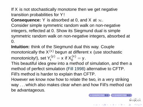
If X is not stochastically monotone then we get negativetransition probabilities for Y !Consequence: Y is absorbed at 0, and X at ∞.Consider simple symmetric random walk on non-negativeintegers, reflected at 0. Show its Siegmund dual is simplesymmetric random walk on non-negative integers, absorbed at0.Intuition: think of the Siegmund dual this way. Couplemonotonically the X (x) begun at different x (use stochasticmonotonicity!), set Y (y)
t = x if X (x)0 = y .
This beautiful idea grew into a method of simulation, and then amethod of perfect simulation (Fill 1998) alternative to CFTP.Fill’s method is harder to explain than CFTP.However we know now how to relate the two, in a very strikingway . . . which also makes clear when and how Fill’s method canbe advantageous.
EXERCISE 9.1 EXERCISE 9.2

FMMR
The alternative to CFTP is Fill’s algorithm (Fill 1998; Thonnes1999), at first sight quite different, based on the notion of astrong uniform time T (Diaconis and Fill 1990) and related toSiegmund duality. Fill et al. (2000) establish a profound link.We explain using “blocks” as input-output maps for a chain.
First recall that CFTP can be viewed in a curiously redundantfashion as follows:
I Draw from equilibrium X (−T ) and run forwards;I continue to increase T until X (0) is coalesced;I return X (0).

Key observation: By construction, X (−T ) is independent ofX (0) and T so . . .
I Condition on a convenient X (0);I Run X backwards to a fixed time −T ;I Draw blocks conditioned on the X transitions;I If coalescence then return X (−T ) else repeat .
Is there a dominated version of Fill’s method?“It’s a kind of magic . . . ”
Queen

Read-once randomness
Wilson (2000a) shows how to avoid a conventional requirementof CFTP, to re-use randomness used in each cycle.A brief description uses the blocks picture.
I input-output maps from Markov chain coupling;I Sub-sample to produce “blocks”, positive probability p (say,
p > 1/2) of block being coalescent;I Algorithm: repeatedly apply blocks. After first coalescent,
return values prior to coalescents.DISPLAY
Key: view simple Small-Set CFTP as composition ofGeometrically many kernels (conditioned to miss small set).
EXERCISE 8.1

CFTP for many samples
Mostly people want many samples not just one. Murdoch andRosenthal (2000) consider various strategies for using samplepaths produced by CFTP etc as effectively as possible:
1. Repeated CFTP: repeat CFTP followed by T0 more values.Independence!
2. Forward coupling: run forwards to coalescence, thenrepeat using coalesced value as initial start. Not CFTP!
3. Concatenated CFTP: use coalesced value from one CFTPto define path for next CFTP. MA(1) structure!
4. Guaranteed time CFTP: like concatenation, but extractonly the last Tg steps of each path. MA(1) structure!
All the CFTP methods have similar costs if care is taken overparameters: decide whether you need independence! Forwardcoupling (or other non-CFTP methods) may be better ifperfection is not a requirement.These ideas led rapidly to the FMMR formulation . . . .

CFTP for many samples
Mostly people want many samples not just one. Murdoch andRosenthal (2000) consider various strategies for using samplepaths produced by CFTP etc as effectively as possible:
1. Repeated CFTP: repeat CFTP followed by T0 more values.Independence!
2. Forward coupling: run forwards to coalescence, thenrepeat using coalesced value as initial start. Not CFTP!
3. Concatenated CFTP: use coalesced value from one CFTPto define path for next CFTP. MA(1) structure!
4. Guaranteed time CFTP: like concatenation, but extractonly the last Tg steps of each path. MA(1) structure!
All the CFTP methods have similar costs if care is taken overparameters: decide whether you need independence! Forwardcoupling (or other non-CFTP methods) may be better ifperfection is not a requirement.
These ideas led rapidly to the FMMR formulation . . . .

CFTP for many samples
Mostly people want many samples not just one. Murdoch andRosenthal (2000) consider various strategies for using samplepaths produced by CFTP etc as effectively as possible:
1. Repeated CFTP: repeat CFTP followed by T0 more values.Independence!
2. Forward coupling: run forwards to coalescence, thenrepeat using coalesced value as initial start. Not CFTP!
3. Concatenated CFTP: use coalesced value from one CFTPto define path for next CFTP. MA(1) structure!
4. Guaranteed time CFTP: like concatenation, but extractonly the last Tg steps of each path. MA(1) structure!
All the CFTP methods have similar costs if care is taken overparameters: decide whether you need independence! Forwardcoupling (or other non-CFTP methods) may be better ifperfection is not a requirement.These ideas led rapidly to the FMMR formulation . . . .

There is something tragic about the enormous numberof men there are in England at the present momentwho start life with perfect profiles, and end by adoptingsome useful profession.
— Oscar Wilde,Phrases and Philosophies for the use of the Young

Lecture 10: Sundry further topics in CFTP
Stult’s Report:Our problems are mostly behind us.
What we have to do now is fight the solutions.
Sundry further topics in CFTPPrice of perfectionEfficiencyImpractical CFTPGeometric ErgodicityImpractical domCFTP theorem

The price of perfection
What kind of price might we have to pay for the perfection ofCFTP?
Propp and Wilson (1996) bound for monotonic CFTP on a finitepartially ordered space: if ` is longest chain, T ∗ is coalescencetime, and
d(k) = maxx ,y
{distTV(P(k)x , P(k)
y )} . (26)
then CFTP is within a factor of being as good as possible:
P [T ∗ > k ]
`≤ d(k) ≤ P [T ∗ > k ] . (27)
EXERCISE 10.1
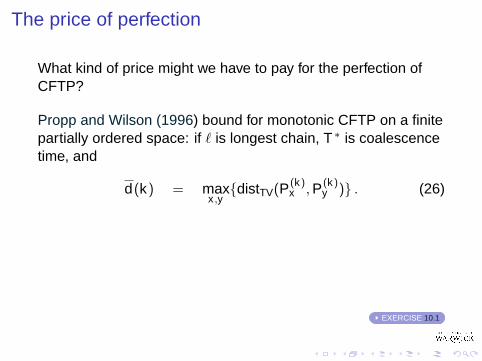

Efficiency
(Co-adapted) CFTP is limited by rate of co-adaptedcoupling: we expect both this and rate of convergence toequilibrium to be exponential.
Let τ be the coupling time, X = (X1, X2) the coupled pair.
Suppose |pt(x1, y)− pt(x2, y)| ≈ c2 exp(−µ2t)while P [τ > t |X (0) = (x1, x2)] ≈ c exp(−µt)
By the coupling inequality, coupling cannot happen fasterthan convergence. Can it be slower? Burdzy and Kendall(2000) show that the answer is yes.

Coupling of couplings
Letting X = (X1, X2), x = (x1, x2),
|pt(x1, y)− pt(x2, y)| =
= |P [X1(t) = y |X1(0) = x1]− P [X2(t) = y |X2(0) = x2]|
≤|P [X1(t) = y |τ > t , X (0) = x ]− P [X2(t) = y |τ > t , X (0) = x ]|
× P [τ > t |X (0) = x ]
Let X ∗ be a coupled copy of X but begun at (x2, x1):
|P [X1(t) = y |τ > t , X (0) = x ]− P [X2(t) = y |τ > t , X (0) = x ] |= |P [X1(t) = y |τ > t , X (0) = x ]−
P [X ∗1 (t) = y |τ > t , X ∗(0) = (x2, x1)] |
≤ P [σ > t |τ > t , X (0) = x ] (≈ c′ exp(−µ′t))
for σ the time when X , X ∗ couple. Thus µ2 ≥ µ′ + µ.

Coupling of couplings
Letting X = (X1, X2), x = (x1, x2),
|pt(x1, y)− pt(x2, y)| =
= |P [X1(t) = y |X1(0) = x1]− P [X2(t) = y |X2(0) = x2]| ≤|P [X1(t) = y |τ > t , X (0) = x ]− P [X2(t) = y |τ > t , X (0) = x ]|
× P [τ > t |X (0) = x ]
Let X ∗ be a coupled copy of X but begun at (x2, x1):
|P [X1(t) = y |τ > t , X (0) = x ]− P [X2(t) = y |τ > t , X (0) = x ] |= |P [X1(t) = y |τ > t , X (0) = x ]−
P [X ∗1 (t) = y |τ > t , X ∗(0) = (x2, x1)] |
≤ P [σ > t |τ > t , X (0) = x ] (≈ c′ exp(−µ′t))
for σ the time when X , X ∗ couple.
Thus µ2 ≥ µ′ + µ.

Coupling of couplings
Letting X = (X1, X2), x = (x1, x2),
|pt(x1, y)− pt(x2, y)| =
= |P [X1(t) = y |X1(0) = x1]− P [X2(t) = y |X2(0) = x2]| ≤|P [X1(t) = y |τ > t , X (0) = x ]− P [X2(t) = y |τ > t , X (0) = x ]|
× P [τ > t |X (0) = x ]
Let X ∗ be a coupled copy of X but begun at (x2, x1):
|P [X1(t) = y |τ > t , X (0) = x ]− P [X2(t) = y |τ > t , X (0) = x ] |= |P [X1(t) = y |τ > t , X (0) = x ]−
P [X ∗1 (t) = y |τ > t , X ∗(0) = (x2, x1)] |
≤ P [σ > t |τ > t , X (0) = x ] (≈ c′ exp(−µ′t))
for σ the time when X , X ∗ couple. Thus µ2 ≥ µ′ + µ.

Impractical CFTP
When can we conceive of being able to do classic CFTP?
Theorem 10.1 (Foss and Tweedie 1998)(Impractical) classic CFTP is equivalent to uniform ergodicity.
Definition 10.2 (Uniform Ergodicity)The chain X is uniformly ergodic, equilibrium distribution π, ifthere is a constant V and γ ∈ (0, 1),
‖P(n)(x , ·)− π(·)‖TV ≤ Vγn for all n, x . (28)
Hint: uniform ergodicity is equivalent to the entire state-spacebeing small, therefore one can use small-set CFTP!
So what is the scope of domCFTP? How far can we go?

Geometric Ergodicity
Definition 10.3 (Geometric Ergodicity)The chain X is geometrically ergodic, equilibrium distribution π,if there is a π-almost surely finite V : X → [0,∞] and γ ∈ (0, 1),
‖P(n)(x , ·)− π(·)‖TV ≤ V (x)γn for all n, x . (29)
Equivalently
Definition 10.4 (Geometric Foster-Lyapunov Criterion)There are: a small set C; constants α ∈ (0, 1), b > 0; and ascale or drift function Λ : X → [1,∞) bounded on C;such that for π-almost all x ∈ X
E [Λ(Xn+1) | Xn = x ] ≤ αΛ(x) + b I [x ∈ C] . (30)
. . . and there are still other kinds of ergodicity!

Impractical domCFTP theorem
Theorem 10.5 (Kendall 2004)(Impractical) domCFTP is possible in principle for anygeometrically ergodic Markov chain.
IDEA: try to use Equation (30)
E [Λ(Xn+1) | Xn = x ] ≤ αΛ(x) + b I [x ∈ C] .
to determine a dominating process Y , dominating in the sensethat
X � Y if and only if Λ(X ) ≤ Y .
The two sets of ingredients of the proof run as follows . . .

Ingredients I
Use Markov’s inequality and coupling to build Y so if Λ(x0) ≤ y0
P [Λ(Xn+1) ≥ y | Xn = x0] ≤ P [Yn+1 ≥ y | Yn = y0] .
Deduce from geometric Foster-Lyapunov criterion that
P [Yn+1 ≥ y | Yn = y0] = αy0/y
whenever y > αy0 , y > max{Λ|C}+ b/α ,
Add a lower reflecting barrier for Y : then ln(Y ) can be relatedto system-workload for a D/M/1 queue, Exponential(1) servicetimes and arrival intervals ln(1/α).

Ingredients II
I If e−1 ≤ α ≤ 1 then D/M/1 queue is not positive-recurrent!
I Fix this by sub-sampling (geometric Foster-Lyapunovcondition is essentially unaltered by this).
I Exact formulae for the D/M/1 equilibrium and dualprocess transition kernel allow us to obtain explicit, simple,simulation algorithms!
I Run D/M/1 queue backwards in time till it hits barrier,which defines a small set for target chains. (Need tosub-sample again so that this small set is of order 1.)
I Simple lemma: coupling of X , Y persists through small-setregeneration.

Ingredients II
I If e−1 ≤ α ≤ 1 then D/M/1 queue is not positive-recurrent!I Fix this by sub-sampling (geometric Foster-Lyapunov
condition is essentially unaltered by this).
I Exact formulae for the D/M/1 equilibrium and dualprocess transition kernel allow us to obtain explicit, simple,simulation algorithms!
I Run D/M/1 queue backwards in time till it hits barrier,which defines a small set for target chains. (Need tosub-sample again so that this small set is of order 1.)
I Simple lemma: coupling of X , Y persists through small-setregeneration.

Ingredients II
I If e−1 ≤ α ≤ 1 then D/M/1 queue is not positive-recurrent!I Fix this by sub-sampling (geometric Foster-Lyapunov
condition is essentially unaltered by this).I Exact formulae for the D/M/1 equilibrium and dual
process transition kernel allow us to obtain explicit, simple,simulation algorithms!
I Run D/M/1 queue backwards in time till it hits barrier,which defines a small set for target chains. (Need tosub-sample again so that this small set is of order 1.)
I Simple lemma: coupling of X , Y persists through small-setregeneration.

Impractical domCFTP: conclusion
I This kind of domCFTP may be un-implementable for any ofseveral reasons:
I use of sub-sampling: implies substantial knowledge ofhigher-order transition probabilities!
I how to implement the Markov inequality coupling?(especially in case of sub-sampling!)
I depends on a Foster-Lyapunov condition which mayproduce a coupling which is much weaker than a moresophisticated approach.
I But it is closely linked to applications of domCFTP whichactually work, such as the perpetuities example in §8.5.

Conclusion
We can predict everything, except the future.