lectures on real options: part iii — some applications
TRANSCRIPT

LECTURES ON REAL OPTIONS:
PART III — SOME APPLICATIONS AND
EXTENSIONS
Robert S. Pindyck
Massachusetts Institute of TechnologyCambridge, MA 02142
Robert Pindyck (MIT) LECTURES ON REAL OPTIONS—PART III August, 2008 1 / 46

Introduction
Now turn to some applications and extensions of themethodology developed so far.
Valuing an undeveloped offshore oil reserve, and determiningwhen it should be developed.Operating options: The option to shut down a factory whenproduction is unprofitable, and the option to resume productionlater.Sequential investment: Investment decisions made sequentiallyand in a particular order.Jump processes: Key variable (e.g., price, value of a project)makes discrete jumps up or down. For example, a copper minemight be expropriated, or a machine might break down.
Robert Pindyck (MIT) LECTURES ON REAL OPTIONS—PART III August, 2008 2 / 46

Valuing Undeveloped Oil Reserves
An undeveloped oil reserve is like a call option. It gives theowner the right to acquire a developed reserve by paying thedevelopment cost.
When to develop the reserve? Same as deciding when toexercise a call option.
The higher the uncertainty over future oil prices, the morevaluable is the undeveloped reserve, and the longer we shouldwait to develop it.
Use of option theory focuses attention on nature and extent ofuncertainty.
Robert Pindyck (MIT) LECTURES ON REAL OPTIONS—PART III August, 2008 3 / 46

Comparison of Stock Call Option and Undeveloped
Petroleum Reserve
Stock Call Option Undeveloped Reserve
Current stock price Current value of developed reserve
Variance of rate of Variance of rate of change of thereturn on the stock value of a developed resource
Exercise price Development Cost
Time to expiration Relinquishment requirement
Riskless rate of interest Riskless rate of interest
Dividend Net production revenue lessdepletion
Robert Pindyck (MIT) LECTURES ON REAL OPTIONS—PART III August, 2008 4 / 46
Valuing Undeveloped Oil Reserves
Undeveloped oil reserve is an option to ”buy” a developed oilreserve, so first step is to determine value of developed reserve.
Value will depend on price of oil.
Price of oil fluctuates stochastically, so value of developedreserve will also fluctuate.
Once we know the stochastic process for the value of developedreserve, use option theory to value the undeveloped reserve.
Robert Pindyck (MIT) LECTURES ON REAL OPTIONS—PART III August, 2008 5 / 46

Valuing Undeveloped Oil Reserves (continued)
1. Value of Developed Reserve
B = number of barrels of oilV = value per barrelR = rate of return to owner of reserveP = price of a barrel of oilΠ = After-tax profit from producing and
selling a barrel of oilµ = risk-adjusted expected rate of return on oilω = fraction produced each year = .10
Production cost ≈ .3P , tax rate ≈ .34,
so Π = (1− .34)(.7)P = .45P
V =∫ ∞
0ωΠe−(r+ω)tdt =
ω(.45P)r + ω
=.045P
.14= .32P
Robert Pindyck (MIT) LECTURES ON REAL OPTIONS—PART III August, 2008 6 / 46

Valuing Undeveloped Oil Reserves (continued)
Depletion of reserve: dB = −ωBdt
Return dynamics: Rdt = ωBΠdt + d(BV )= ωBΠdt + BdV −ωBVdt
Return is partly random: Rdt/BV = µdt + σdz ,
where dz = ε√
dt
µBVdt + σBVdz = ωBΠdt + BdV −ωBVdt,so dV = µVdt −ω(Π− V )dt + σVdz
Therefore: dV = (µ− δ)Vdt + σVdz , where δ is payout ratenet of depletion:
δ = ω(Π− V )/V ≈ .04
Robert Pindyck (MIT) LECTURES ON REAL OPTIONS—PART III August, 2008 7 / 46

Valuing Undeveloped Oil Reserves (continued)
2. Value of Undeveloped Reserve
Given process for V , value of undeveloped reserve, we can nowdetermine value of developed reserve.
Let F (V , t) = value of 1-barrel unit of undeveloped reserve.
By setting up risk-free portfolio, etc., can show that F mustsatisfy:
12σ2V 2 ∂2F
∂V 2+ (r − δ)V
∂F
∂V− rF = −∂F
∂t
Robert Pindyck (MIT) LECTURES ON REAL OPTIONS—PART III August, 2008 8 / 46
Valuing Undeveloped Oil Reserves (continued)
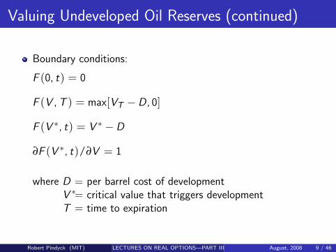
Boundary conditions:
F (0, t) = 0
F (V , T ) = max[VT −D, 0]
F (V ∗, t) = V ∗ −D
∂F (V ∗, t)/∂V = 1
where D = per barrel cost of developmentV ∗= critical value that triggers developmentT = time to expiration
Robert Pindyck (MIT) LECTURES ON REAL OPTIONS—PART III August, 2008 9 / 46

Valuation Example
Developed reserve expected to yield 100 million barrels of oil;
The present value of the development cost is $11.79 per barrel;
The development lag is 3 years;
Relinquishment is after a period of 10 years;
Standard deviation of value of developed reserves is 14.2 percent;
The payout ratio (net production revenues/value of reserves) is4.1 percent; and
The value of the developed reserve today is $12 per barrel.
Step 1: Calculate the present value of a developed reserve (V′):
V′= e−(.041)×3 × $12 = $10.61 per barrel.
Step 2: Calculate the ratio of reserve value to development cost, C:C = V′/D = $10.61/$11.79 = .90.
Robert Pindyck (MIT) LECTURES ON REAL OPTIONS—PART III August, 2008 10 / 46

Valuation Example (continued)
Step 3: Calculate the value of the undeveloped reserve:
Value = (Option Value per $1 Development Cost (from Table)) ×(Total Development Cost) = (0.05245) × ($1179.0 million) =$61.84 million.
Hence, although reserve cannot be profitably developed undercurrent conditions, the right to develop it in the future is worthmore than $60 million.
If you believe standard deviation of value of developed reserve is25% instead of 14%, value of undeveloped reserve is muchhigher.
So determining standard deviation is critical!
Robert Pindyck (MIT) LECTURES ON REAL OPTIONS—PART III August, 2008 11 / 46

Oil Price Uncertainty (90% Probability Range)
Robert Pindyck (MIT) LECTURES ON REAL OPTIONS—PART III August, 2008 12 / 46
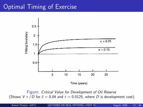
Optimal Timing of Exercise
Figure: Critical Value for Development of Oil Reserve(Shows V ∗ /D for δ = 0.04 and r = 0.0125, where D is development cost)
Robert Pindyck (MIT) LECTURES ON REAL OPTIONS—PART III August, 2008 13 / 46

Option Values per $1 of Development Cost
σv = 0.142 σv = 0.25
V/D T=5 T=10 T=15 T=5 T=10
0.80 0.01810 0.02812 0.03309 0.07394 0.0103920.85 0.02761 0.03894 0.04430 0.09174 0.123050.90 0.04024 0.05245 0.05803 0.11169 0.143900.95 0.05643 0.06899 0.07458 0.13380 0.16646
1.00 0.07661 0.08890 0.09431 0.15804 0.190711.05 0.10116 0.11253 0.11754 0.18438 0.216641.10 0.13042 0.14025 0.14464 0.21278 0.244241.15 0.16472 0.17242 0.17599 0.24321 0.27349
Source: Siegel, Smith, and Paddock (1987).
Note: Because option values are homogeneous in the development cost,
total option value is the entry in the table times the total development
cost.Robert Pindyck (MIT) LECTURES ON REAL OPTIONS—PART III August, 2008 14 / 46

Undeveloped Reserve Values (in $ Millions)
σ = 14.2% σ = 25%
V/D T=5 T=10 T=15 T=5 T=10
0.70 7.72 15.59 20.09 52.83 83.460.80 21.34 33.15 39.01 87.18 122.520.90 47.44 61.84 68.42 131.68 169.661.00 90.32 104.81 111.19 186.33 224.851.10 153.77 165.35 170.53 250.87 287.96
Note: This table uses a payout ratio of 4.1 percent and 100 Million Bbls of Oil.
Robert Pindyck (MIT) LECTURES ON REAL OPTIONS—PART III August, 2008 15 / 46

Is GBM the Right Model of Price?
Figure: Log Price of Crude Oil and Quadratic Trend Lines
Robert Pindyck (MIT) LECTURES ON REAL OPTIONS—PART III August, 2008 16 / 46

Mean Reversion in Oil Price
Consider the following mean-reverting process for the value of adeveloped oil reserve:
dV = η (V − V ) V dt + σ V dz . (1)
Then the partial differential equation for value of undevelopedreserve, F (V , t), is
12 σ2
v V 2 FVV + [r − µ + η(V − V )] V FV − r F = −Ft (2)
If the time until relinquishment is long enough (more than fiveyears), we can ignore the time dependence of F (V , t), so thatthe term −Ft disappears.
As we saw, solution can be written using the confluenthypergeometric function, which has a series representation.
Can use this solution, with different values for η and V , todetermine the extent to which mean reversion matters.
Robert Pindyck (MIT) LECTURES ON REAL OPTIONS—PART III August, 2008 17 / 46

Mean Reversion in Oil Price (continued)
Wey (1993) has shown, using a 100-year series for the real priceof crude oil, that a reasonable estimate for η is about 0.3, andthat using this value (and a value of σv of .20), the extent towhich mean reversion matters depends on the value to which Vreverts, V , relative to the development cost, D.
If V is much larger than D, accounting for mean reversion givesa larger value for the undeveloped reserve when V < D becauseV is expected to rise over time. Wey shows that if V is abouttwice as large as D, ignoring mean reversion can lead one toundervalue the reserve by 40 percent or more.
On the other hand, if V is about as large as D, ignoring meanreversion will matter very little.
Robert Pindyck (MIT) LECTURES ON REAL OPTIONS—PART III August, 2008 18 / 46

Operating Options
You own a factory that produces widgets: 1000/month for thenext 10 years.
Variable cost of production is C = $10 per widget.
The price of widgets is now P = $15, but P will fluctuate overtime.
What is the value of this factory?
In each month, you have an option to produce 1000 widgets andreceive $1000P . For each option, the exercise price is 1000C =$10,000.
You have 10 x 12 = 120 European call options, one for eachmonth.
Let Fn(P) denote the value of the option to produce 1000widgets in month n when the current price of widgets is P .
Robert Pindyck (MIT) LECTURES ON REAL OPTIONS—PART III August, 2008 19 / 46

Operating Options (continued)
Then the value of this factory is simply the sum of the values ofthe 120 options, i.e., it is:
V = F1(P) + F2(P) + ... + F120(P)The Black-Scholes formula (modified for dividends) can be usedto value each Fn(P). To do this, one must determine the driftand volatility for P .
Assume
dP/P = αdt + σdz
Let µ = risk-adjusted expected return on P .
Then δ = µ− α is the “return shortfall.” It is equivalent to adividend rate in the modified Black-Scholes formula. To findFn(P), just reduce P by the present value of the“dividends”,and apply the standard B-S formula.
Robert Pindyck (MIT) LECTURES ON REAL OPTIONS—PART III August, 2008 20 / 46

Operating Options (continued)
For example, suppose P = $15, α = 0, µ = r . Then, δ = r , tofind, say, F12(P), i.e., the value of the option to produce oneyear from now, replace P with
P ′ = P − rP/(1 + r) = P/(1 + r)
and then use the standard B-S formula:
F12 = P ′N(d1)− Ce−rTN(d2)
where d1 = ln(P ′/C )+(r+σ2/2)Tσ√
T, and d2 = d1 − σ
√T
Here N(.) is the cumulative probability distribution function fora standardized normal distribution. Also, T = 1 if we arelooking at the option to produce one year from now.
Robert Pindyck (MIT) LECTURES ON REAL OPTIONS—PART III August, 2008 21 / 46

Sequential Investment
Many investment decisions are made sequentially, and in aparticular order.
Oil production capacity: Find reserves, then develop them.New line of aircraft: Engineering, prototype production, testing,final tooling.Drug development: Find new molecule, Phase I testing, PhaseII, Phase III, construct production facility, marketing.Any investment that can be halted midway and temporarily orpermanently abandoned.
Like a compound option; each stage completed (or dollarinvested) gives the firm an option to complete the next stage (orinvest the next dollar).
Robert Pindyck (MIT) LECTURES ON REAL OPTIONS—PART III August, 2008 22 / 46

Sequential Investment (continued)
Example: two-stage investment in new oil production capacity.
First, obtain reserves, through exploration or purchase, at costI1.Second, Build development wells, at cost I2.Begin with option, worth F1(P), to invest in reserves. Investinggives the firm another option, worth F2(P), to invest indevelopment wells.Making this second investment yields production capacity, worthV (P).
Work backwards to find the optimal investment rules.
Robert Pindyck (MIT) LECTURES ON REAL OPTIONS—PART III August, 2008 23 / 46

Investment Rule for a Two-Stage Project
Project, once completed, produces one unit of output per periodat an operating cost C .
Output can be sold at price P, which follows a GBM:
dP = α P dt + σ P dz . (3)
Production can be temporarily suspended when P falls below C ,and resumed when P rises above C , so profit flow isπ(P) = max [P − C , 0].
Investing in first stage requires sunk cost I1, and second stagerequires sunk cost I2.
Robert Pindyck (MIT) LECTURES ON REAL OPTIONS—PART III August, 2008 24 / 46

Investment Rule for a Two-Stage Project (con’t.)
Solve the investment problem by working backwards:
First, find value of completed project V (P).Next, find value of option to invest in second stage, F2(P), andcritical price P∗
2 for investing.
Then, find value of option to invest in first stage, F1(P), andcritical price P∗
1 .
Robert Pindyck (MIT) LECTURES ON REAL OPTIONS—PART III August, 2008 25 / 46

Investment Rule for a Two-Stage Project (con’t.)
Value of the Project. V (P) must satisfy
12 σ2 P2 V ′′(P) + (r − δ) P V ′(P)− r V (P) + π(P) = 0 , (4)
subject to V (0) = 0, and continuity of V (P) and VP(P) atP = C . Solution is:
V (P) ={
A1 Pβ1 if P < C ,B2 Pβ2 + P/δ− C/r if P > C .
(5)
where
β1 = 12 − (r − δ)/σ2 +
√[(r − δ)/σ2 − 1
2
]2 + 2r/σ2 > 1,
β2 = 12 − (r − δ)/σ2 −
√[(r − δ)/σ2 − 1
2
]2 + 2r/σ2 < 0.
Robert Pindyck (MIT) LECTURES ON REAL OPTIONS—PART III August, 2008 26 / 46

Investment Rule for a Two-Stage Project (con’t.)
Constants A1 and B2 found from continuity of V (P) and V ′(P) atP = C :
A1 =C 1−β1
β1 − β2
(β2
r− β2 − 1
δ
)(6)
B2 =C 1−β2
β1 − β2
(β1
r− β1 − 1
δ
)(7)
Robert Pindyck (MIT) LECTURES ON REAL OPTIONS—PART III August, 2008 27 / 46

Investment Rule for a Two-Stage Project (con’t.)
Second-Stage Investment. Find value of option to invest insecond stage, F2(P), and critical price P∗
2 .
Value of option must satisfy
12 σ2 P2 F ′′
2 (P) + (r − δ) P F ′2(P)− r F (P) = 0 (8)
subject to the boundary conditions
F2(0) = 0 (9)
F2(P∗2 ) = V (P∗
2 )− I2 (10)
F ′2(P
∗2 ) = V ′(P∗
2 ) (11)
Robert Pindyck (MIT) LECTURES ON REAL OPTIONS—PART III August, 2008 28 / 46
Investment Rule for a Two-Stage Project (con’t.)
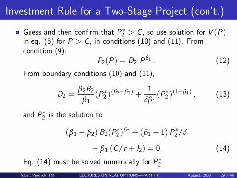
Guess and then confirm that P∗2 > C , so use solution for V (P)
in eq. (5) for P > C , in conditions (10) and (11). Fromcondition (9):
F2(P) = D2 Pβ1 . (12)
From boundary conditions (10) and (11),
D2 =β2B2
β1(P∗
2 )(β2−β1) +1
δβ1(P∗
2 )(1−β1) , (13)
and P∗2 is the solution to
(β1 − β2) B2(P∗2 )β2 + (β1 − 1) P∗
2 /δ
− β1 (C/r + I2) = 0. (14)
Eq. (14) must be solved numerically for P∗2 .
Robert Pindyck (MIT) LECTURES ON REAL OPTIONS—PART III August, 2008 29 / 46
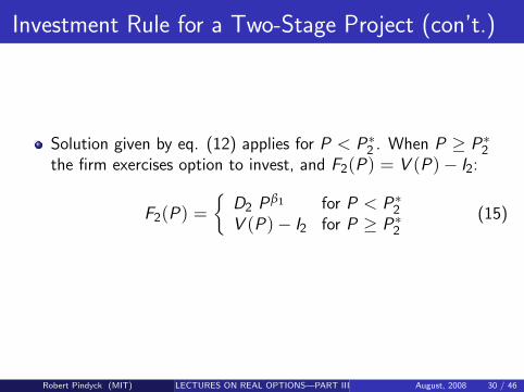
Investment Rule for a Two-Stage Project (con’t.)
Solution given by eq. (12) applies for P < P∗2 . When P ≥ P∗
2the firm exercises option to invest, and F2(P) = V (P)− I2:
F2(P) ={
D2 Pβ1 for P < P∗2
V (P)− I2 for P ≥ P∗2
(15)
Robert Pindyck (MIT) LECTURES ON REAL OPTIONS—PART III August, 2008 30 / 46
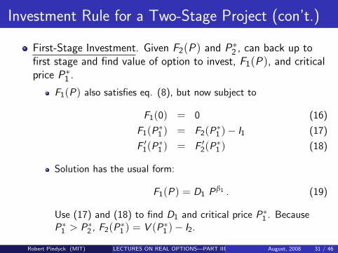
Investment Rule for a Two-Stage Project (con’t.)
First-Stage Investment. Given F2(P) and P∗2 , can back up to
first stage and find value of option to invest, F1(P), and criticalprice P∗
1 .
F1(P) also satisfies eq. (8), but now subject to
F1(0) = 0 (16)
F1(P∗1 ) = F2(P∗
1 )− I1 (17)
F ′1(P
∗1 ) = F ′
2(P∗1 ) (18)
Solution has the usual form:
F1(P) = D1 Pβ1 . (19)
Use (17) and (18) to find D1 and critical price P∗1 . Because
P∗1 > P∗
2 , F2(P∗1 ) = V (P∗
1 )− I2.
Robert Pindyck (MIT) LECTURES ON REAL OPTIONS—PART III August, 2008 31 / 46

Investment Rule for a Two-Stage Project (con’t.)
Since P∗1 > P∗
2 , and since the investment can be completedinstantaneously (before P can change), we know that once P reachesP∗
1 and the firm invests, it will complete both stages of the project.This result seems anti-climactic, so why bother to solve thistwo-stage problem? Why not simply combine the two stages?
First, real-world investing takes time, so firms often do completeearly stages and then wait before proceeding with later stages.
Second, the two stages may require different technical ormanagerial skills, may be located in different countries, or maybe subject to different tax treatments. For these reasons onefirm may sell a partially completed project to another. Ourmethod lets us value a partially completed project.
Third, we will apply this approach to problems wherecompletion of the project takes time.
Robert Pindyck (MIT) LECTURES ON REAL OPTIONS—PART III August, 2008 32 / 46

Critical Prices and Option Values for Two-Stage
Project
Robert Pindyck (MIT) LECTURES ON REAL OPTIONS—PART III August, 2008 33 / 46

Investment Rule for a Two-Stage Project (con’t.)
Extension to projects with three or more stages: Start at theend and work backwards, using solution for each stage in theboundary conditions for the previous stage. Value of option toinvest in any stage j of an N-stage project is of the form
Fj (P) = Dj Pβ1 ,
and the coefficient Dj and critical price P∗j are found by solving
equations (13) and (14), with P∗j replacing P∗
2 andIj + Ij+1 + . . . + IN replacing I2.
Robert Pindyck (MIT) LECTURES ON REAL OPTIONS—PART III August, 2008 34 / 46

Introduction to Jump Processes
Sometimes uncertainty is discrete in nature.
Competitor enters with better product, making yours worthless.
New regulations make your factory worth less (or more).
Sudden, unexpected success in the laboratory.
Foreign operation is expropriated, or tax treatment changed.
War, financial collapse, pestilence, etc.
As long as these discrete events are non-systematic(diversifiable), easy to handle.
Model as jump (Poisson) process, dq. Analogous to Wienerprocess:
dq ={
0 with probability 1− λ dtu with probability λ dt.
where u is the size of the jump (and can be random).Robert Pindyck (MIT) LECTURES ON REAL OPTIONS—PART III August, 2008 35 / 46

Simple Example: Value of a Machine
Suppose a machine produces constant flow of profit, π, as longas it operates.
First, assume it lasts forever and never fails. No risk. Then assetreturn equation is:
rVdt = πdt
and value of machine is V = π/r .
Robert Pindyck (MIT) LECTURES ON REAL OPTIONS—PART III August, 2008 36 / 46

Simple Example: Value of a Machine (con’t.)
Now suppose at some point machine will break down and haveto be discarded. So value of the machine follows the process:
dV − Vdq
where dq is a jump (Poisson) process. Now asset returnequation is:
rVdt = πdt + E(dV ) = πdt − λVdt
Thus,
V =π
r + λ.
So just increase discount rate by λ.
Robert Pindyck (MIT) LECTURES ON REAL OPTIONS—PART III August, 2008 37 / 46

Undeveloped Oil Reserve
Back to undeveloped oil reserve. Recall that value of developedreserve followed the process:
dV = (µ− δ)Vdt + σVdz
where δ is payout rate net of depletion:
δ = ω(Π− V )/V ≈ .04
Now suppose a developed reserve is subject to full or partialexpropriation. Then V follows:
dV = (µ− δ)Vdt + σVdz − Vdq
where dq is a jump process with mean arrival rate λ, and
E(dzdq) = 0.
Robert Pindyck (MIT) LECTURES ON REAL OPTIONS—PART III August, 2008 38 / 46

Undeveloped Oil Reserve (con’t.)
If “event” occurs, q falls by a fixed percentage φ (with0 ≤ φ ≤ 1). Thus V fluctuates as a GBM, but over each dtthere is a small probability λdt that it will drop to (1− φ) timesits original value, and then continue fluctuating until anotherevent occurs.
Robert Pindyck (MIT) LECTURES ON REAL OPTIONS—PART III August, 2008 39 / 46

How to Estimate Arrival Rate λ?
Begin with estimate of expected time T for event to occur, e.g.,5 years.
Now get equation for E(T ). Probability that no event occursover (0, T ) is e−λ T . So probability that the first event occurs inthe short interval (T , T + dT ) is e−λ T λ dT . So expected timeuntil V jumps is:
E [T ] =∫ ∞
0λ T e−λT dT = 1/λ
So if expected T is 5 years (60 months), use 0.2 (.01667) for λ.
Robert Pindyck (MIT) LECTURES ON REAL OPTIONS—PART III August, 2008 40 / 46

Optimal Investment Rule
Want to find F (V ), value of undeveloped reserve, and optimalexercise point V ∗.As we saw earlier, the dz component of dV can be “replicated.”We assume dq is non-systematic, i.e., can be diversified. So userisk-free rate. Then return equation is:
rFdt = E(dF ) .
Expand dF :
r F dt = (µ− δ)VF ′(V )dt + 12 σ2 V 2 F ′′(V )dt−
λ { F (V )− F [(1− φ) V ] } dt .
Can rewrite this as:
12 σ2V 2F ′′(V ) + (r − δ)VF ′(V )− (r + λ)F (V )+
λF [(1− φ)V ] = 0 .
The same boundary conditions apply as before.Robert Pindyck (MIT) LECTURES ON REAL OPTIONS—PART III August, 2008 41 / 46
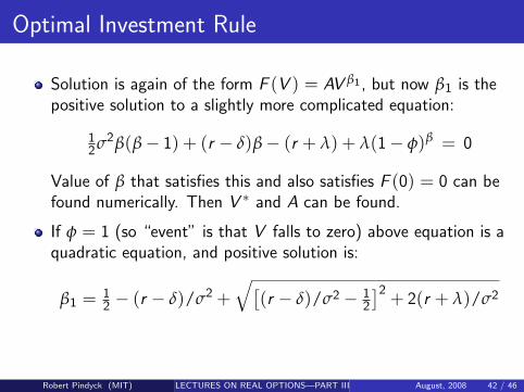
Optimal Investment Rule
Solution is again of the form F (V ) = AV β1 , but now β1 is thepositive solution to a slightly more complicated equation:
12σ2β(β− 1) + (r − δ)β− (r + λ) + λ(1− φ)β = 0
Value of β that satisfies this and also satisfies F (0) = 0 can befound numerically. Then V ∗ and A can be found.
If φ = 1 (so “event” is that V falls to zero) above equation is aquadratic equation, and positive solution is:
β1 = 12 − (r − δ)/σ2 +
√[(r − δ)/σ2 − 1
2
]2 + 2(r + λ)/σ2
Robert Pindyck (MIT) LECTURES ON REAL OPTIONS—PART III August, 2008 42 / 46

Optimal Investment Rule (con’t.)
Table shows β1, V ∗, and a for various values of λ, for case ofφ = 1. A positive value of λ affects F (V ) in two ways.
First, it reduces the expected rate of capital gain on V (from αto α− λ), which reduces F (V ).
Second, it increases variance of changes in V , which increasesF (V ).
As the Table shows, net effect is to reduce F (V ), and thusreduce the critical value V ∗.
Net effect is strong; small increases in λ lead to big drop in V ∗.
Robert Pindyck (MIT) LECTURES ON REAL OPTIONS—PART III August, 2008 43 / 46
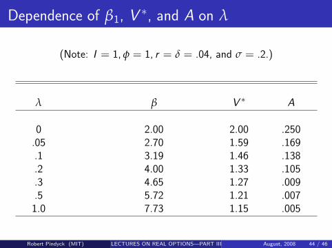
Dependence of β1, V ∗, and A on λ
(Note: I = 1, φ = 1, r = δ = .04, and σ = .2.)
λ β V ∗ A
0 2.00 2.00 .250.05 2.70 1.59 .169.1 3.19 1.46 .138.2 4.00 1.33 .105.3 4.65 1.27 .009.5 5.72 1.21 .0071.0 7.73 1.15 .005
Robert Pindyck (MIT) LECTURES ON REAL OPTIONS—PART III August, 2008 44 / 46
Optimal Investment Rule (continued)
Note that we increased λ while holding α = µ− δ fixed. Couldargue that the market-determined expected rate of return on Vshould remain constant, so that an increase in λ is accompaniedby a commensurate increase in α (otherwise no investor wouldhold this project).
Suppose φ = 1. If α increases as much as λ so α− λ isconstant, we have to replace the terms (r − δ) in equation for βwith (r + λ− δ). Then an increase in λ is like an increase inthe risk-free rate r , and leads to an increase in F (V ) and V ∗.
Robert Pindyck (MIT) LECTURES ON REAL OPTIONS—PART III August, 2008 45 / 46

Optimal Investment Rule (continued)
The simple jump process we used leads to a differential equationfor F (V ) that is easy to solve. Could specify different processfor V .
Firm holding a patent faces competitors, each trying to developits own patent. Success of a competitor might cause V to fallby a random, rather than fixed amount. Over time additionalcompetitors may enter, so V continues to fall.Calculation of optimal investment rule is more difficult, andwould require numerical solution method.
Robert Pindyck (MIT) LECTURES ON REAL OPTIONS—PART III August, 2008 46 / 46