leeeeeeeeeeeee lfllflflflflflfllflfl ellllelleeeiie postgraduate school o monterey, california.01...
TRANSCRIPT

V-Ml?G U9 FOUNATIONS OF THE uINTELIGENCE MODLE OF lIE EIIA ulRESECH ROM (Mli.)(U) Nivin POSTAUTE SCHOL
MNUTEREY CA 6 L SMITH SEP 6UCLASSIFIEDF O154 N
EEEIIEEEllEEEEIllf fl l....llflIIIEEIhhIII
lEEEEEEEEEEEEElfllflflflflflfllflflEllllEllEEEIIE

.%
] 1125 14 ill6
III 1
L 7-
11111 IL',45
J1* J
" ' "i W. '''''- "' """ .' ' '. ' " "' -." " ""' " " '. "' '"' ." -''" i " "" -"- " ". " . ''.".' -. ..-" " ." ."I- '- ''.," -,,,,' .' ",. ,".r .. ,,.. .. J.,F. ,'... 1,.A,' ..... ,. ' .. '.. ' .". ... . ,,. ' .- -. .-'.'-"."."" . '
/ .' ,o'L, , . , . '. -- -, ', . . . ,. '- .' '- .' ." . ' -- v * " .- C '' " - -. , . . . . . . -- - - - , - '
.. . ..

NAVAL POSTGRADUATE SCHOOLo Monterey, California
.01
JAiv 2
IO THESISAFOUNDATIONS OF THE INTELLIGENCE MODULE
OF THE AIRLAND RESEARCH MODEL
(ALARM)
by
Gaylon L. Smith
September 1986
Thesis Advisor: Samuel H. Parry
Approved for public release; distribution is unlimited.
C~.4
87 121 o54
Z t 14 ) 7 .- . s' - -- -
SECURITY CLASSIFICATION OF THIS PAGE
REPORT DOCUMENTATION PAGEla REPORT SECURITY CLASSIFICATION lb. RESTRICTIVE MARKINGS
UNCLASSIFIED 'p
2a SECURITY CLASSIFICATION AUTHORITY 3 DISTRIBUTION/AVAILABILITY OF REPORTApproved for public release; distribution
2b DECLASSIFICATION /DOWNGRADING SCHEDULE is unlimited.
4 PERFORMING ORGANIZATION IPORT NUMBER(S) S MONITORING ORGANIZATION REPORT NUMBER(S) ,..'
6a. NAME OF PERFORMING ORGANIZATION 6b OFFICE SYMBOL 7a. NAME OF MONITORING ORGANIZATION(If applicable)
Naval Postgraduate School Code 55 Naval Postgraduate School6c ADDRESS (City, State, and ZIP Code) 7b. ADDRESS (City, State, and ZIP Code)
Monterey, California 93943-5000 Monterey, California 93943-5000
8a NAME OF FUNDING/SPONSORING 8b. OFFICE SYMBOL 9. PROCUREMENT INSTRUMENT IDENTIFICATION NUMBERORGANIZATION (If applicable)
8c ADDRESS (City, State, and ZIP Code) 10 SOURCE OF FUNDING NUMBERSPROGRAM PROJECT TASK WORK UNITELEMENT NO NO NO ACCESSION NO
11 TITLE (Include Security Classification)
FOUNDATIONS OF THE INTELLIGENCE MODULE OF THE AIRLAND RESEARCH MODEL (ALARM)
12 PERSONAL AUTHOR(S)
Smith, Gaylon L.31a TYPE OF REPORT 13b TIME COVERED 14 DATE OF REPORT (Year, Month, Day) 15 PAGE COUNT
Master's Thesis FROM TO 1986 Seotember 96'6 SUPPLEMENTARY NOTATION
COSATI CODES 18 SUBJECT TERMS (Continue on reverse if necessary and identify by block number)
PELD GROUP SUB-GROUP AirLand Battle, ALARM, AirLand Research Model,Intelligence Module
9 ABSTRACT (Continue on reverse of necessary and identify by block number)
This thesis lays the foundation for the Intelligence Module of the AIRLAND RESEARCHMODEL (ALARM). It examines the relationship between the Intelligence Module and theother modules of ALARM. Specifically it develops the structure of the IntelligenceModule to include the flow of combat information from other modules, the fusion ofcombat information into tactical intelligence and the subsequent dissemination of thatintelligence. Additionally, it proposes a Lanchester-type formulation for targetacquisition and presents a methodology to estimate the required coefficients from theoutput of a high resolution combat simulation.
. S'"3jT ON AVAILABILITY OF ABSTRACT 21 ABSTRACT SECURITY CLASSIFICATIONt..%CLASSIFEDtjNLMITED 0 SAME AS RPT 0 ]TIC uSERS UNCLASSIFIED
..a ,%1ME OF RESPONSIBLE 'NDiVIDUAL 22b TELEPHONE (Include AreaCode) 22c O'(.E S'MB0.
Samuel H. Parry (408) 646-2779 Code 55PyDD FORM 1473, 84 MAR 83 APR edition may be used -nti eu"haued SECURITY CLASSIFICATO N 0; S :L, __
All other edit-ons are obsolete
1
e..P --. .. e.I -

Approved for public release; distribution is unlimited.
Foundations of the Intelligence Moduleof the AirLand Research Model
(ALARM)
by
Gaylon L. SmithMajor, United States Army
B.A., Saint Louis University, 1972
Submitted in partial fulfillment of therequirements for the degree of
MASTER OF SCIENCE IN OPERATIONS RESEARCH
from the
NAVAL POSTGRADUATE SCHOOLSeptember 1986
Author: ____n" ylon L. Smith
Approved by:AA
Peter Purdue, Chairmian,Department of Operations Research
Kneale T. Marshall,Dean of Information and Policy Scien
2
., . . . .. . . . • , . . • . . . . . ..... ,. . .. C.? . ., ,'; , ,y , , , - , % , ,:;,£ .. ,, -- .-.-- .- ..,,... ....,,. ,,,, ,.,. .., .". . . . .. . .. . ..

ABSTRACT
This-thesis lays the foundation for the Intelligence Module of the AIRLAND
RESEARCH MODEL (ALARM). It examines the relationship between the
Intelligence Module and the other modules of ALARM. Specifically it develops the
structure of the Intelligence Module to include the flow of combat information from
other modules, the fusion of combat information into tactical intelligence and the
subsequent dissemination of that intelligence. Additionally it proposes a
Lanchester-type formulation for target acquisition and presents a methodology to
estimate the required coefficients from the output of a high resolution combat
simulation. , '
QIJJ
3
-A-._
' A" le/

.'% IN 170. - -.- % Ca
TABLE OF CONTENTS
I. INTRODUCTION .......................................... 9A. PURPOSE AND ORGANIZATION OF THE THESIS ........... 9B. CHARACTERISTICS OF THE AIRLAND
BATTLEFIELD....................................... 10
% C. THE AI RLAND RESEARCH MODEL (ALARM) ........... 11I
IL. DEVELOPMENT OF AN INTELLIGENCE MODEL .............. 17A. AN OVERVIEW OF THE TACTICAL INTELLIGENCE
*SYSTEM ............................................ 17B. THE INTELLIGENCE MODULE ........................ 21
AC. THE INTELLIGENCE ESTIMATE....................... 25
D. SUMMARY ......................................... 26
Ill. THE COMBAT INFORMATION PROCESSOR.................. 27A. TARGET VECTORS................................... 27B. DETERMINING THE PERCEIVED TARGET SIZE .......... 30C. AGGREGATING TARGETS ............................ 33D. COMMUNICATION OF COMBAT INFORMATION
BETWEEN CIPS...................................... 371. Subordinate to Senior Reporting........................ 372. Senior to Subordinate Reporting........................ 38
E. SUMMARY ......................................... 39
IV A G T A Q I I I N . . . . .. . . . . . . . . . . . . . .4
A.MOELN TARGET ACQUISITION...... ...................... 40
B. ACQUISITIONMODELS .............................. 42
1. The Glimpse Model.................................. 42
2. The Continuous Search Model ......................... 44* 3. The Glimpse and Continuous Search Models in a
Simulation....................................... 46C. LANCH ESTER'S EQUATIONS AND ALARM...............47
'SD. LANCIIESTER'S LAWS OF COMBAT.................... 47.4
4

1. First Linear Law (Direct Aimed Fire) ...................... 47
2. Second Linear Law (Area Firing) .......................... 49
3. Square Law ........................................... 51
E. MODEL EXTENSIONS ................................... 521. Extensions for Replacement Rate .......................... 52
2. Range Dependent Acquisition Coefficients .................. 533. Fraction of Force Which is Effective ....................... 54
F. HETEROGENEOUS FORCES .............................. 56
V. DETERMINATION OF ACQUISITION COEFFICIENTS ........... 59
A. THE ACQUIS!TION-RATE COEFFICIENT'SRELATIONSHIP TO ACQUISITION TIME .................. 59
B. JUSTIFICATION FOR USING THE RECIPROCAL OFTHE TIME TO ACQUIRE ................................. 60I. Acquisition as a Continuous Time Markov-Chain ............ 60
2. Development of The Forward Kolmogorov Equations ......... 60
3. Distribution of Times Between Acquisitions ................. 62
C. MAXIMUM LIKELIHOOD ESTIMATION OFACQUISITION-RATE COEFFICIENTS ..................... 64
D. THE RATE AT WHICH ACQUIRED AN ACQUIREDTARGET RETURNS TO THE UNACQUIRED STATE ........ 67
E. SU M M A RY ............................................. 68...
VI. THE INTELLIGENCE MODULE AND DECISION-MAKINGIN A LA R M .................................................. 69A. A. DECISION-MAKING IN ALARM ....................... 69
B. A W ORKED EXAM PLE .................................. 71
1. Scenario .............................................. 72
2. Initial Situation, t = 0 .................................. 72
3. Situation at t = I ...................................... 76
4. Situation at t = 2 ...................................... SO5. Situation at t = 3 ...................................... S 3
6. Situation at t = 4 ...................................... S5
C . SU M M A R Y ............................................. IS
VII. SUMMARY/FUTURE DIRECTIONS ............................ 92
A . SU M M A R Y ............................................. ' 2
5

B. FUTURE DIRECTIONS................................ 93
LIST OF REFERENCES............................................ 94
-,INITIAL DISTRIBUTION LIST...................................... 95
--o
C'
.o
4o
'C.
Co.
Rb
-a'. ..... 2 ... '_ . J2 "°-,2 .'°... . "".. ::P" " ", . . ."."-. ."-. .'.'.". •. .-.-.. '.'J-° '. .".•

LIST OF TABLES
1. TYPICAL AREAS OF INFLUENCE .......................... 18'p2. TYPICAL AREAS OF INTEREST............................ 19
3. MATCHING OF TARGETS ................................ 334. REPORTING THRESHOLDS ............................... 385. INITIAL ABIP OF COMBAT UNITS.......................... 72
-97
-9%

LITOF FIGURES
1.1 Modular Structure of ALARM ................................. 131.2 Division Planning Sub-Module ................................. 14K.1.3 Unit Planning .............................................. 152.1 Areas of Interest and Influence ................................. 202.2 Information Flow ........................................... 22
2.3 ALARM Modules ........................................... 233.1 Functions of the Intelligence Module ............................ 283.2 CIP Logic Flow............................................. 294.1 Cardoid Function ........................................... 56
6.1 Diagram of Battlefield ........................................ 736.2 Situation At t = 0 .......................................... 74
6.3 Projected Power Curves for Initial Plans........................... 756.4 Perceived Power Curves For t= 0 .............................. 77
6.5 Situation at t ....1......................................... 786.6 Perceived Power Curves for t = I1............................... 806.7 Situation at t =2 ........................................... 816.8 Perceived Power Curves For t= 2 .............................. 836.9 Situation at t= 3 ........................................... 856.10 Perceived Power Curves for t = 3 ............................... 86
6.11 Situation at t = 4 ........................................... 876.12 Perceived Power Curves for t 4 4............................... 896.13 Adjusted Perceived Power Curves for t 4 4..........................90
... . . . .

I. INTRODUCTION
A. PURPOSE AND ORGANIZATION OF THE THESISThis thesis lays the foundation for the Intelligence Module of the AIRLAND
RESEARCH MODEL (ALARM). It examines the relationship between the
Intelligence Module and the other modules of ALARM. Specifically it develops the
the structure of the Intelligence Module to include the flow of combat information
from other modules, the fusion of combat information into tactical intelligence and the
subsequent dissemination of that intelligence. Additionally it proposes a
Lanchester-type formulation for target acquisition and presents a methodology to
estimate the required coefficients from the output of a high resolution combat
simulation. The thesis is organized as follows:
1. Review of the AirLand Battlefield and the AIRLAND RESEARCH MODEL
(ALARM).
2. Overview of the current tactical intelligence system of the U.S. Army.
3. Development of the Intelligence Module of ALARM.
4. Discussion of the functions of the Combat Intelligence Processor and
methodologies for implementing them.
5. Review of the Glimpse and Continuous-search models of target acquisition.
6. Modeling target acquisition using a Lanchester-type formulation.
7. Estimation of Lanchesterian coefficients using maximum likelihood estimators.
8. Illustration of the inter-relationships between the Intelligence, Execution and
Planning Modules of ALARM using a worked example.
9. Discussion of areas requiring additional research/study.
The thesis is concerned with modeling the tactical intelligence system of the
United States ground forces at the corps level and below. It concentrates on U.S. Army
forces employed in the European Theater against Soviet forces. Models of the Sovict
tactical intelligence system will not be explored. lowever, it is anticipated that many of'
the basic constructs developed in this thesis can be applied with a rinimum of'
modification in future studies. Similarly the acquisition of combat information b- U.S.
Air Force assets will be addressed in the research being done on the Air Voice
. . . . .

sub-module of ALARM. Finally, although an important source of combat information
and intelligence, echelons above corps are not specifically addressed in this thesis.
Before continuing with the development of the Intelligence Module the
characteristics of the AirLand Battlefield are examined and the structure of the
AIRLAND RESEARCH MODEL, as currently envisioned, is reviewed.
B. CHARACTERISTICS OF THE AIRLAND BATTLEFIELD
The U.S. Army Field Manual 100-5 [Ref. l:pp. 1-1,1-2] lists eight characteristics
that will distinguish the airland battlefield:
1. Nonlinear Maneuver Battles - The U.S. Army will face enemy forces which are
highly mechanized and possess very sophisticated and lethal weapon systems.
The enemy forces will integrate armored ground forces with air power and the
potential use of nuclear/chemical weapons. Both sides will be able to rapidly
mass troops and fires in order to achieve penetrations. As a result distinct lines
of battle, which have characterized past wars and many current models, will be
the exception.
2. Lethal Systems - Both the U.S. and enemy forces will possess weapons of high
quality and lethality. The coordinated use of air and ground precision guided
munitions will allow the concentration of combat power at critical points on the
battlefield.
3. Sensors and Communications. - The wide-spread availability of surveillance and
target acquisition sensors, coupled with an extensive communications system,
will allow rapid dissemination of combat information and tactical intelligence.
This will affect both the range and scope of the battle.
4. Nuclear and Chemical Warfare - The potential use of nuclear and or chemical
weapons will drastically alter the battlefield. The threat of' their use will preclude
the massing of troops, except for short periods. It is possible that tactical
nuclear weapons will come to dominate the battle and relatively small maneuerforces will be used to exploit their effects. The tempo of the battleiheld ill
increase while the duration of specific battles will decrease.
5. Command and Control - Effective command and control will be a dc ii\c
factor in future battles. Ironically, the vulnerability of conmmunication stc:,
to electronic countermeasures may significantly degrade the commander, a!1;::t%
to conmmunicate with, and subsequently control, his forccs at critical Jutctw:c,
in the battle. Conmand and control facilities will be specificaly targeted.
-C'.(
• I .
o,

6. Air Systems - The use of helicopters and tactical air power will extend the depth
of the battle. The effective use of air defense will become an important issue in
future battles.
7. Austere Support - Future battles will be fought at the end of long and
vulnerable supply lines. The ability of both sides to strike deep will hamper
resupply to the fighting forces. Additionally the nonlinear, maneuver oriented
battlefield will preclude the stockpiling of supplies in any great quantities.
8. Rear Area Combat - Support systems in the rear area will be the focus of
intense attacks intended to disrupt the flow of crucial supplies, replacements
and information. The goal will be to reduce the effectiveness of the fighting
forces by denying them needed support. Additionally, maneuver forces will be
siphoned from the main battle area in order to provide protection to rear area
support facilities.
These characteristics describe a battlefield which is potentially very different from
those of the recent past. New operational and tactical doctrines have been and are in
the process of being developed. These new doctrinal concepts are being explored using
field training exercises (FTX's), command-post exercises (CPX's), wargames and
computer simulations. Many of the combat models (computer simulations) which are
currently in use are modifications of dated models. ALARM is an attempt to explore
new methodology based on what is believed to the true nature of the modern
battlefield.
C. THE AIRLAND RESEARCH MODEL ( ALARM)
ALARM will be used initially to model the interdiction battle at the corps level
and below. The interdiction battle is the foundation of the U.S. Army's AirLand Battle
doctrine. Three primary purposes have been identified for ALARM [Ref. 21:
1. The development of modeling methodology appropriate for the very large scale
but sparsely populated rear areas involved in the (non-FLOT) interdiction
battle, and for the conmand and control of the Airland Battle force.
2. The application of these methodologies in the construction of a
simulation'wargaming model initially focusing on two-sided interdiction.
3. The eventual use of the model to perform research on the conduct of the total
AirLand Battle.
~~I1
j.-I

E'. The goal of the development effort is to produce a systemic model which will
allow for a detailed audit trail by which an analysis of the cause and effect relationships
can be conducted. ALARM has the following unique features:
1. Systemic architecture which allows the model to conduct the simulation without
the-roquirement for human intervention at critical decision points.
2. Rule-based decision systems in which the command and control (C2 ) functionsare automated, along with related processes.
3. A Network representation which uses a generalized network methodology andmultidimensional coordinate systems to represent terrain, transportation andcommunication interconnections, and command and control relationships.
4. A Generalized Value System (GVS) which is the base concept for the future
state decision making featured in the model. The GVS assigns an initial value
to a combat unit based on the availability of weapons, personnel and supplies.
This initial value is then adjusted (discounted) to reflect the time delay that may
be required before the unit is in position to accomplish its assigned mission. The
initial values of logistic/support units and other battlefield entities are
determined primarily from their ability to increase the value of combat units.
Extensive research on the GVS has been conducted by Kilmer. [Ref. 31
ALARM is a testbed for examining methodology; it is not a production model.
The proposed computer model of ALARM, as currently conceived, has three major
components: a Planning Module, an Execution Module and an Intelligence Module.
These modules are currently being developed. Figure 1.1 displays a simplified diagram
of the relationship between the three modules. The Planning Module includes the
decision algorithms and consists of several submodules. Figure 1.2 shows a division
;. planning sub-module in more detail. There is a planning sub-module for each
hierarchical level of the task force organization (battalion through corps), to include,
as required, associated sub-modules for indirect fire, engineering, logistics, U.S. Army
aviation, maintenance etc.
The planning sub-modules develop detailed plans for execution using decision
algorithms and available information from the Execution Module. Figure 1.3 displays
the stages in a planning sub-module for a single U.S. unit and the interaction between
the planning sub-module and the Execution Module. Briefly, the unit receives the
commander's guidance, which usually consists of the higher headquarters plan for the
12
.- 7

4._
zz
LIL
Figure 1.1 M rStructure oALARM.
operation and some specific directives f'or its implementation. Courses of action are
developed and feasibility checks conducted. A detailed plan of action is then prcpared',-o which is sent to the Execution Module. In the Execution Module the plan parameters
':" 13
' 4S_.
4. . . . 4.. '-..... 4..~ S ., ,. * ~ p. .2.Q* ~ . ~ '~ S - '.~h~k ~ ~ ~ AX z

LALU-
1--I
L.<
,€ z1.9X
I,-=
z,
r0
,UZ Z.
0- 0
.. Figure 1.2 Division Planning Sub-Module.
• are initially checked to insure that they conform to the commanders guidance. During
' the execution, decision threshold parameters are monitored. Violation of a decision
threshold parameter may cause the planning cycle to be re-entered and the plan
> QD
%14
".-
- .r *- *.~,, - ___ ___

modified. Current research is concentrating on developing the Planning Module, the
planning sub-modules which comprise it, and the inter-relationships between the
various sub-modules.
PLANNING MODULE INTELLIGENCEMODULE
RECEIVE GUIDANCE& FORMULATECOURSE OF ACTION
INTELLIGENCEESTIMATE
4-.-
CONDUCT I I UPATEFEASIBILITY PERCEIVEDCHECKS DATA BASE
COMPLETEPLAN
EXECUTIONMODULE
-YESPARAMETERSR VIOLATED ?/K ILT INFORMATION
NO
EXECUTION HALTEXECUTION
Figure 1.3 Unit Planning.
1
15
._
SI

It is apparent that the Intelligence Module plays a key role in the interactionbetween the Planning Module and the Execution Module. The Intelligence Modulereceives raw data (combat information) concerning enemy forces and other modelentities from the Execution Module. It then must separate this information and pass it
* along to the appropriate level in the Planning Module. For instance, during theexecution of a division operation it must determine what information should be madeavailable to each battalion and brigade planning sub-module (to include their relatedsupport planning sub-modules). This availability of information may be a function ofthe unit's location on the battlefield, task force organization, and unit composition andstrength. One important issue concerns whether this information should represent the"ground truth" or some perceived truth. If the data is to be transformed, how should
this be accomplished ? This issue is addressed later in the thesis.
A second function. of the Intelligence Module, which is not apparent from thefigures, is the preparation of an intelligence estimate. This intelligence estimate is anintegral part of the planning module. Thus each hierarchical level which possesses anintelligence analysis capability has an intelligence sub-module associated with itsplanning sub-module. These intelligence sub-modules are responsible for the fusion ofexisting intelligence and combat information into a intelligence estimate which can beused by the planning sub-module. The intelligence system and the development of amodel is addressed next.
16

1I. DEVELOPMENT OF AN INTELLIGENCE MODEL
A. AN OVERVIEW OF THE TACTICAL INTELLIGENCE SYSTEMThe AirLand Battle concept of interdiction, or the deep battle, is extremely
dependent upon accurate and timely information about enemy units and battlefield*conditions. The tactical intelligence system is responsible for the collection and
evaluation of information the and dissemination of intelligence to the tactical decision
maker. First it is necessary to clarify the distinction between information, combatinformation and tactical intelligence.
* Def. INFORMATION - unevaluated material including that derived fromobservations, communications, reports, rumors, imagery or any other source. Theinformation may or may not be true, accurate and/ or even pertinent.Information can also be negative in the sense that an event may have not
occurred, or that an item of interest is absent from the battlefield.* Def COMBAT INFORMATION - information upon which minimal verification
and validation has been conducted. It is characterized by being readilyexploitable, near real-time delivery from source to user, and used immediately for
tactical execution and fire support.- Def: TACTICAL INTELLIGENCE - the product resulting from the collection,
evaluation and interpretation of information. The goal of tactical intelligence isto minimize the uncertainty concerning the enemy's objectives, capabilities and
battlefield conditions which may effect the accomplishment of the mission. It ischaracterized as all-source, complex and a result of detailed analysis. It isdelivered in hours, and used for planning.
The tactical intelligence system focuses the intelligence effort by delimitingcollection and evaluation responsibilities for each subordinate unit and by setting
priorities for information upon which collection is to be concentrated.o Def" ESSENTIAL ELEMENTS OF INFORMATION (EEl) - those critical
items of information about the enemy and battlefield needed by the commanderto assist him in reaching a logical decision. ELI are often time sensitive.
17
......... ...........

EEl requirements are generally provided to the unit from its superior
headquarters. Additional EEl, which support its specific mission, may be developed by
the unit itself. Collection efforts are centered on satisfying these EEl requirements.
To further enhance the collection effort each tactical unit is assigned ageographical. area for intelligence operations. This geographical area is subdivided into
an Area of Influence and an Area of Interest.
0 Def. AREA OF INFLUENCE - that portion of the assigned area of operation inwhich the commander can directly affect the course of the battle using his ownorganic and supporting assets.
The actual area will vary in size depending upon the terrain, enemy capability
and disposition, and the unit's ability to react to enemy actions. The area is specified in
terms of time. Normally, a commander will possess the means for monitoring and
collecting combat information within the area of influence. Table 1 displays typical
area of influence assignments for various levels of command.
TABLE I
TYPICAL AREAS OF INFLUENCE
Level of Time Beyond FLOTcommand or Atta~k Objectives
Battalion up to 3 hoursBrigade up to 12 hoursl)ivision up to 24 hoursCorps up to 72 hours
In addition to an area of influence each unit has an area of interest.
Def. AREA OF INTEREST - includes the area of influence and extends beyond
and laterally to those areas in which encmv units or battlefield conditions are
capable of affecting a unit's mission in the near future.
Again the area of interest is specified in terms of time and assigned after
considering the terrain, enemy and the unit's status. I nlike the area ofinfluence a unit
does not normally have the capability of monitoring its area of interest. Rather. the
IS

unit receives information about the area of interest primarily from higher and adjacent
units. Table 2 displays typical area of interest assignments for various levels of
command.
TABLE 2
TYPICAL AREAS OF INTEREST
Level of Time Beyond FLOTCommand or Attack Objectives
Battalion up to 12 hoursBrigade up to 24 hoursDivision up to 72 hoursCorps up to 96 hours
Figure 2.1 shows the inter-relationship of the areas of influence and interest for
a corps. The key feature is the stacking of the areas of influence and interest of a
subordinate unit within the area of influence of the next higher unit. Each unit is
responsible for collecting information within its area of influence. The means to do this
are the organic and supporting assets. The primary information collectors at each level
are detailed below:
* Battalion: Tank/Infantry companies, the scout platoon, ground surveillance radar
(GSR) sections, and artillery fire support teams (FIST) are the usual collectors.
* Brigade: Divisional brigades generally do not possess organic assets for the
collection of information. Rather, they task their subordinate battalions to
perform the required collection of information within the brigade's area of
influence.
* Division: In addition to subordinate brigades, the cavalry squadron, military
intelligence battalion, divisional artillery target acquisition units, NBC
reconnaissance platoon, air defence battalion and divisional engineer and aviation
units are the primary collectors.
* Corps: In addition to subordinate divisions and separate brigades the normal
collectors are armored cavalry regiments, artillery units, nilitary intelligence
groups, aviation groups, engineers and adjacent corps.
19

1 /77 <x7\(4
/ .
\XL \~-* " w '/ N61
/ '7 w\4\Y
\N
NX
.4.J
pe ..... X
... .. .D. .
LUL
U..
LU"D
0a-
* C
0 U- Z' -
- . - . - -- - - -C.~K.~<:.>y a\A : -w :. . . a . <.. D% < . < N - ... a

Figure 2.2 is a simplified diagram of the flow of information, combat information
and intelligence into and out of a unit intelligence organization. Information flows into
the intelligence section from collectors which are operating in the unit's area of
influence. The intelligence section identifies combat information contained in the rawinformation and passes this to the commander, associated staff elements, subordinateunits and the senior units intelligence section as appropriate. The intelligence section
also receives combat information from all of these same agencies. This combat
information is disseminated as required and, coupled with intelligence from the senior
headquarters, is used to prepare and update the intelligence estimate. This intelligenceestimate is essential to the commander and his staff in planning and conducting
operations.
Two unique features of the intelligence system are illustrated in Figure 2.2. First,unlike combat information, intelligence only flows down the chain of command.
Subordinate units do not pass intelligence to senior units. This may seem like anunreasonable constraint on the flow of critical information, but in reality it is merely
an artifice of the distinction between combat information and intelligence. Tacticalintelligence is combat information which has been processed and specifically tailored tothe unit's mission. It is necessarily limited in scope and contains suppositions about the
enemy. There actually tends to be a healthy, but unofficial, dialogue between
intelligence organizations about enemy capabilities and potential actions. The secondunique feature is that information does not flow exclusively into the intelligence
section. Information flows into the commander and the other staff sections of the unit.
This information receives mninimal processing (verification/ validation) and then enters
the intelligence system as combat information.With this as a basis for understanding the tactical intelligence system, the next
step is to construct a model which replicates the functions and results of the system.
B. THE INTELLIGENCE MODULE
The architecture of the proposed Intelligence Module and its relationships with
the Planning Module and Execution Module is displayed in Figure 2.3 'Notice that the
Planning Module is structured so that there is a sub-planning module f-or each
hierarchical level of the organization. The Intelligence Module is sub-divided along the
same lines. Associated with each sub-planning module is an intelligence sub-miodule.
Each intelligence sub-module consists of two components; the Combat Inf'ormiation

q-7.T711 T 3-17-- -. --
INTELL COMBATINFO
SENIOR UNIT
I NTELLI GENCE"
ORGINIZATION
I NTELL COMBAT
S-COMMANDER I NTELL UNITUNIT
INF AND INTELLIGENCESTAFF ELEMENTS COMBA RCOMBAT ORGANIZATION
A INFO I
NFO
UNIT UNIT UNITCOLLECTOR COLLECTOR CO.ECTOR
INFORMATION
COLLECTOR COLLECTOR OLLECTCR
Figure 2.2 Information Flow.
Processor (CIP) and the Intelligence Estimate Processor (IEP). All information, bothfriendly and enemy, is routed to a CIP. Updates in friendly unit status such as location
or strength, the destruction of a bridge and contact with an enemy unit are examples of
information which could be received from the Execution Module.
.'......,,,.. ..,,.-. .... . ....-........ '..2.... .............. "....... .-

I NTELL
PROCESSING ( INFO I
COMBAT . CMBATCCMAT ( CORPS ) (CORPS)
PLANS INTELL COMBAT
PRCESII NFOLE
Maing COMBAT PeSI COMlBAT II-- ..O (D o .) .(DIV.)
I I FILTERED FILTERED
PLANS IN'TELL COMBAT ( COMBAT~~INFO |INFO OIC
INT'ELL r y'
Figur 3 RMCESSING Mo sINFOPlanninlg ¢CMBAT (COM.) B (AT .
INF
PLANS INTELL .C.MBAT
Ba IolPOESN INFO S_.._X
.JPlanning COMBAT PROESNG COMBAT O
Execution OuutMdule (TaggeM D Source) I
Figure 2.3 ALARMI Modules.
In order to illustrate the proposed model a typical item of combat information
will be traced through the system, in this case a sighting of a group of enemy tanks
reported by a battalion's GSR. Information from the Execution Module is tagged by,
23

the collector which is reporting the information. This collector is identified on the task
force hierarchical network as belonging to a particular unit. This task force tag is used
to route the information to the correct battalion CIP. In the CIP the incoming
information is compared to the current perceived data base. The CIP must determine if
the reported- group of tanks is a first time sighting of a previously unknown enemy
unit, a redundant sighting which has been reported by another collector or an update
on an already known enemy unit. The method by which this checking is conducted and
the aggregation methodology are described in Chapter II I.
Assume that in this specific instance the group of tanks is determined to be a
new target. The CIP updates the battalion's perceived data base by adding the enemy
tanks. This perceived data base is used both by the battalion's planning sub-module
and the IEP component of the battalion's intelligence sub-module. Additionally the
combat information concerning the tanks is passed to the CIPs of the battalion'ssubordinate units and to the CIP of the next senior unit in the task force hierarchy. As
indicated in Figure 2.3 the combat information reported up and down the chain of
command may be filtered. In the downward flow of combat information this filteringserves as a sieve. Aggregated information is broken down into blocks that are
appropriate for the level receiving the combat information. Conversely the filtering
serves to aggregate the combat information which is passed up the task force network.
Thus, for example, battalions would receive data on the location of platoons whereasdivisions would receive data on battalions and regiments. It is currently conjectured
that the EEI, augmented by a standardized set of reporting criteria, will form the basis
for the filtering.
The Intelligence Estimate Processor (IEP) is the second component of theIntelligence sub-module. As previously stated the IEP operates on the perceived data
base of the organization and the intelligence estimate of the next higher unit. The
purpose of the IEP is to prepare an intelligence estimate which will be used by the
planning sub-module of the organization. The spccific purpose of the llP is to idcntil\
cnemy units, by type and designation, and to predict their courses of action. lhis is a
somewhat restricted version of an actual intelligence estimate which would additionally
consider the effhct of terrain on the friendly units ability to accomplish its mission. InALARNI, as currently conceived, the Planning Module will determine the influence of
terrain on the fricndy forces. The IIP will he restricted to cxarmining the encim h'rcec.
Naturally, this will require that the clccts of' terrain on cnenv f'orces also 1c
'p.

determined. It is believed that much of the ongoing effort to develop a terrain network
structure, and the corresponding Planning Module which capitalizes on it, will result in
a model which can be used by the IEP with only minor modifications.
Continuing the example of the detected tanks, the battalion IEP would fuse this
new information with the existing intelligence estimate of the battalion. The IEP will
possess the capability to aggregate enemy units and identify the parent organization.
Potential enemy courses of action will be evaluated and passed to the planning
sub-module. The IEP must specifically estimate the arrival time of the enemy units at
selected points on the battlefield. Additionally the IEP will have a methodology which
will allow it to determine the most lkely enemy course of action. The intelligence
estimate prepared by the IEP will develop the Situational Inherent Power (SIP) Curves
for the enemy forces [Ref. 31. These SIP Curves form the basis for the future state
decision making in ALARM.
Concurrent with the development of the battalion's intelligence estimate, the IEP
of the controlling brigade would be revising its intelligence estimate by incorporating
the new combat information which had been passed to its CIP from the battalion. This
updated brigade intelligence estimate would then flow to the subordinate units of the
brigade and be used to alter their own intelligence estimates as required.
C. THE INTELLIGENCE ESTIMATE
The area of identifying and predicting the enemy's course of action forms the
heart of the intelligence estimation procedure. Currently ongoing research into terrain
modeling and avenue of approach determination in ALARM must be completed before
the intelligence estimation methodology can be developed further. hIowever, a
promising area of research may be to develop a set of decision rules to aggregate,
identitf' and predict enemy activity using "templates". Currently the intelligence ollicer
develops and uses three general types of templates to assist him in preparing the
intelligence estimate [Ref. l:pp. 6-7,6-8]:
I. Doctrinal Templates - models based on enemy tactical doctrine. They portray
frontages, depths, echelon spacing and force composition.
2. Situational Templates - a series of projections that portray how the doctrinal
templates will appear when applied to specific terrain.
3. lvcnt Templates - models of enemy activity. They are sequential projcctions o
events that relate to both space and time on the battlefield. lhey indicate the
enen's ability to adopt a particular course o" action.
25
* ' a -.

The templates are specialized to the enemy and the tactical situation. They are
tools used to assist the intelligence officer, but are at best approximations. Decision
rules based on templates must recognize and adjust for this lack of precision.
D. SUMMARY
The Intelligence Module consists of two components: a Combat Information
Processor (CIP) and a Intelligence Estimate Processor (IEP). Information from the
Execution Module is identified by the collector and flows on the task force
organizational hierarchy network to the appropriate CIP. The CIP updates the
perceived data base and directs the combat information to other task force elements as
required. The Intelligence Estimate Processor (IEP) prepares an intelligence estimate
which identifies enemy units, their locations and courses of actions. The IEP also
develops the SIP curves for the enemy units which is used by the Planning Module.
Intelligence flows down the task force hierarchy. The Intelligence Module serves as the
funnel for all information between the Execution Module and the Planning Module.
'.2
" 26
I-.

1I1. THE COMBAT INFORMATION PROCESSOR
The previous chapter addressed the proposed Intelligence Module and its twocomponents, the Combat Information Processor (CIP) and the Intelligence EstimateProcessor (IEP), in general. This chapter further develops the concept of the CIP, itsrelationships to the Execution Module and IEP. It specifies the information whichmust be passed from the Execution Module and IEP to the CIP and the method bywhich this is accomplished. Figure 3.1 shows the linkages between the ExecutionModule, the CIP and the IEP; the functions of each are indicated. The logic by which
the CIP processes incoming reports is diagrammed in Figure 3.2 The next sectionsdiscuss the internal CIP logic and propose specific methodology.
A. TARGET VECTORSTarget acquisition is performed in the Execution Module and the results passed
to the appropriate CIP by means of a target vector. When a scanning unit acquires an
entity a target vector is created. This target vector is unique and remains in existanceas long as the scanning unit is able to track the entity. A target vector consists of the
following components:* i1, 12 - the entity's true identification code and a target number assigned by the
scanning unit. The identification code, I1, is used by the Execution Module toaddress the correct entity for computations. Each entity on the battlefield willhave a unique identification code number. The target number, k2, is a temporary
identification code used by the CIP and IEP. The targct number is not unique,but rather is created when the entity is acquired. If the entity is "lost" to thescanning unit and subsequently acquired again a new target number is created.
* Xi ... ,Xk - the true current size (number) of each of the elements of which theentity is composed.
N , ...Yk - the current pc.ceived (acquired) siue (number) of each of' the targetelements contained in the entity.
SD i .Dk - the number of target elements which hae been acquired thisiteration.
A , - an activity code which describes the entity's current perceived combat a.tix it%or status. For example possihle combat activiZies are attack, delhend. \kithdra%%.
II
a'..**A~~d'......%.,. ~ ~ ~ ' i

INTELLIGENCE MODULE
IEP CIPIAggregates targets INTELL .. rets & nMaintainsinto organizations Target Vectors2 Matches to Order 2 Aggregates Report';of Battle 3 Directs ComOat ,. \"
3 Evaluates Enemy C info to other CIPs \' /Courses of Action I'
4 Prepares Enemy SIF INFO SourctCurves Leeel
check
EX E C UTKONJi.~lL~iv
= ,rget
nCqUlSn
Figure 3.1 Functions of the Intelligence Module.
delay, movement to contact, tactical movement while not in contact, etc. Status
codes also apply to geographic entities on the battlefield such as bridges, tunnels,
railheads and airfields. These status codes describe the current perceived state of
the geographic entity.
SV- a velocity vector which specifies the speed and direction of the target.
* LI, L2 - the true and perceived location , respectively, of the target. Results from
the Execution Module are always reported based on the true location. The
perceived location results from decision algorithms which aggregate and classify
targets.
28
'p

CIP RECEIVES
INCOMING TARGETIwor / INL
SEARCH EXISTING ANDINCOMING TARGET VECTORSFOR A POSSIBLE MATCH
MATCH FOIW4 YE POXWIh' AGGREGATE TARGETS YES
,NO NO! OI8N JARE
CREATE NEW COMIE T ARGET
TARGET VECTOR VKI
t REPORT COMIBAT INF:O
REPOTING YES TO APPRO)PRIATEOCIP
NO if
Figure 3.2 CIP Logic Flow.
* T - time of the report.
U U - identification code of the unit (sensor) reporting the information. This code
is used to route the report to the correct task-force CIP.
C - a classification code provided by the 1EP. This code has several levels. At the
lowest level it indicates the perceived unit size and type of the target. For
example a tank platoon or motorized rifle battalion. At the intermediate level it
identifies targets which are subordinate units to a larger organization. As an
example three targets are identified as tank companies belonging to the same
* 29
~ $tJ~:{.'~~K \*Kz.S~zKK.:+i.V iK..§-. )

tank battalion. Finally, at the highest level, a target may be identified as being a
mspecific unit listed in the order of battle, e.g., the Is Regiment of the 55 tMotorized Rifle Division. This classification is not necessarily the ground truth,but rat her is the result of the decision algorithms used by the IEP.
Since an acquired target does not necessarily remain acquired the current number
of acquired target elements can eventually decrease to zero. When this happens the
target vector for enemy units is deleted. As acquisition is lost the classification code, C,remains at the highest level reached (unless it is changed by the 1EP). Thus the gradualloss of acquisition represents the degrading of information about a specific target.
Conversely, a target vector for a geographic entity is not deleted when acquisition islost; it remains unchanged from the last observation. Essentially, the information abouta geographic entity's status ages after acquisition is lost and may not be accurate.
B. DETERMINING THE PERCEIVED TARGET SIZEEach CIP will be receiving reports from one or more subordinate units
represented in the Execution Module. The CIP can therefore receive more than one
report about the same target. Each of these reports can differ in the number of target
elements acquired. The CIP must be able to determine the number of target elementswhich have been acquired given the number reported by different subordinate units.
Three simple methods for determining the perceived number of acquired target
elements are proposed.
*Method A :Assume there is no overlap in the reported target elements. That is,each report represents distinct target elements which have not been reported by
any other collector. Under this method the perceived number of target elements
acquired is:
Acquired = min (Di, X'i)(31
where
Di the total number of the ith target elements reported newly acquired this
iteration
=' the true number of target elements remaining unacquircd.
30)

Example 3-1
A CIP has three collectors which report the following number of newly acquired
tanks, from the same target1
d, =6
di --8
dl =10
where
dj' the report about target element I
The true number of unacquired tanks is 20. In this method the perceived number of
newly acquired tanks is:
min (24,20) = 20.
V Method B: Assume that there is maximum overlap in the reported target
elements. Each target element is reported at least once. The largest report is the
upper bound on the number of newly acquired target elements, and the remaining
reports are subsets. The perceived number of target elements acquired is:
Acquired = max(di,... ,di) (3.2)
Example 3-2
Using the data from Example 3-1 the perceived number of acquired tanks is:
max (6,8, 10) = 10.
Method C: Assume that the number of newly acquired target elements is
bounded by the smallest and largest reports. A weighted averaging technique is then
used to determine the perceived number of target elements acquired. Weighting is
required to place emphasis on those reports which are more credible. A simple
weighting factor could be based on the range separating the collector from the
target, the battlefield environment and the sensor type. Consider the followigweighting function:
where
r = range separating the collector and the target
rmax = the maximum range at which the collector is effective
31
U.
t#. ,,r -,1o.,. ''',''...."e .;, " e "" e "- , ". ..". ". .*". ,"_, '. . '-. '. ' '_'.,. .. .. -. .• . " . '. ' .%".'. -
W = l-(r/rmax)g for 0 < r 5 rmax (3.3)
(depends upon battlefield conditions)
g = a shaping constant which is determined for each-collector / target combination (can be adjustedfor battlefield conditions).
The shaping constant, g, may be a function of the attenuation coefficient found in
many high resolution models of target detection.
The perceived number of the ith target element acquired by the jth collector is
given by:
(w X di) / (FWi) (3.4)k pi
Example 3-3As in Example 3-1, each CIP has three collectors reporting to it. Each collector
has the weighting function
Wi = I -(ri,5000)'
The following reports are made:1
d! = 6 r, r= 4500
2dt = 8 ,r 2 = 2000
3di = 10 ,r 3 = 500
The weights are calculated to be:1
W1 = 0.1
2W! = 0.6
W1 = 0.9
The perceived number of acquired tanks is:
[(.1 x 6)+(.6 x S)+(.9 x IW)/[ .1 + .6 + .9 9 .
Of the three methods presented, weightcd a veraging provides the most flexibility.
The perceived number of acquired targets can be casily adjusted For range, battlefield
32

."6 .. . -. , . .TQd r . -,s w.- V- -
conditions and sensor (collector) type. It is important, regardless of the method.5
chosen, that the results are consistent with the target acquisition methodology adopted
for use in the Execution Module.
C. AGGREGATING TARGETS
4, A CiP receives target information from its collectors through the Execution
Module, filtered combat information from senior and subordinate CIPs, and
intelligence from the associated IEP. The CIP must possess an algorithm which
determines if a new target vector should be created or existing target vectors combined
into a single target vector. A modification of a methodology proposed by Lindstrom
can be used to aggregate target vectors when required [Ref. 41. A basic assumption is
that the error in the reported target location follows a circular normal distribution. A
target generally consists of several target elements but is reported as a single location.
The error in question measures the collector's ability to accurately judge the true target
center, not its ability to locate specific target elements. The test is composed of two
steps; a similarity check and a proximity test. If the decision is made to combine the
targets, an adjusted location is calculated. The algorithm is:
TABLE 3
MATCHING OF TARGETS
Incoming Existing Existing Existing
Target Y Target X1 Target X2 Target X3
(Score) (Score) (Score)
Tank Tank (1) Tank (1)
BMP BMP (1) BMP (1)
Arty Arty (1)
ZSU-23 (0)
SA-8 (0)
Rank 3 2 0
13
33
Step 1. Check the incoming target vector against current target vectors for
matches in perceived target element types. The matching algorithm proposed by
Lindstrom searches the existing target vectors for a single match in target element type
between the newly reported target and the existing targets. This algorithm can bemodified slightly to consider a heterogeneous forces composed of several different
target element types. The purpose of the algorithm is to match the incoming targetwith a similar type target. The size of the targets is not considered when attempting to
find a match, this issue is addressed by the aggregation algorithm.
The proposed methodology ranks potential matches between the existing target
vectors and the incoming reported target. Each target element type of the reported
target is compared to each target element type of an existing target vector. For each
target element type match between the two targets a "1" is scored. For each target
element type which is not matched a "0" is scored. The rank of the potential match is
merely the sum of the scores. Ties in the ranks can be resolved by considering such
factors as: terrain, enemy situation and projected enemy courses of action. As the
terrain model and the intelligence estimation procedures are developed the matching
algorithm can be refined to consider more information about the target and potential
matches (e.g. avenues of approach and activity status). Starting with the highest
ranking potential match the proximity test is conducted until an aggregation takes
place, or all matches have been considered. If no matches are found (i.e., all ranks are
0) a new target vector is created. As an example consider the targets vectors shown in
Table 3. The incoming target, Y, is compared to the three existing target vectors, X 1,
X 2 and X3 . Three target element matches are found between Y and X1, two matches
between Y and X2 and no matches between Y and X3. Since X, has the highest rank
it would be considered first when attempting to aggregate targets. If Y and X, were
not combined into a single target the aggregation procedure would next consider X 2.
Finally, if Y and X2 were not combined a new target vector would be created for Y.
Step 2. Conduct the proximity test - The null hypothesis to be tested is that thereported target location means are the same:
0i 1 (1X,/Y) = (I'X2 ' PtY2)II1 : (/IXI PtYl ) (1tx2 ' ltY2
a. Using a table look up, determine the circular error probable (CEP) associated with
each target report and compute the standard deviation for each. The circular normal
34

assumption leads to the following relationship between the CEP and standard
deviation:
Si = CEPi/I.774 (3.5)
b. Calculate the square of the distance between the reported locations.
D2 = X X2 )2 + (Y 1- Y2 )2 (3.6)
c. Compute the test statistic
T = D2 (o+ (3.7)1 62.
(note T is distributed 2. = exponential (X = 1/2)..X
d. If T < 2(C) then accept Ho and combine target vectors.
e. If targets are combined calculate location as:
X= {X X (rI + s2)/2} + {X, x (r2 + s,)/2} (3.8)
Y'= (Y x (r, + 2)/12} + Y2 x(r 2 + sl)/2} (3.9)
where
r= (size of target 1)/ (size of target 1 + size of target 2)
r2 = (size of target 2) / (size of target I + size of target 2)
S1 = Fl/(' l +72)
2= 2(1 + 2)
The size of a target is measured as the number of primary fighting elements thatit has. The ratio of the sizes, r, and r2, act as a weighting factors. Without the,
weighting factors it would be possible for a small target, which has a relatively small
CEP associated with it, to dominate when calculating the adjusted position. Similarl.x.
s and s act as weighting factors which compensate Ior the CEIP ofeach target.
S35
S,,S.5
°%
....... .

Example 3-4
A battalion CIP receives an intelligence update from its associated IEP. The IEP,based on an intelligence estimation procedure, indicates that there is a motorized rifle
company, consisting of BMPs and tanks, located in the vicinity of cartesian coordinates
(550,765). The CEP for this type and size of unit is assumed to be 200 meters, for the
purpose of the example.
* Step 1. Checking the existing target vectors the battalion CIP identifies a
potential target consisting of 4 BMPs and 2 tanks located at (400,700) with aCEP of 150 meters. The selected target vector has a rank of two since it matches
both target element types of the incoming target vector.
Step 2.
a. Compute the associated standard deviations.
= 200/ 1.774 = 112.74(2= 150/ 1.774 = 84.55
b. Calculate the square of the distance between the reported locations.
D 2 - (550-400)2 + (765-700)2 = 26725
c. Compute the test statistic.
T = 26725/(12710.31 + 17148.70)= 1.352
d. Using the relationship between the X2 and the
exponential (1/2) distributions, the .95th quantile is given by:
Q.95= -2 In (l-a) = 5.991 (3.10)
since T = 1.35 < Q.95 = 5.99
do not reject the null hypothesis and combine the targets.
e. The combined target location is calculated by
r1 = 10(10 + 6) = 0.63
r2 = 6,(10 + 6) = 0.38
S,= 112.74,(112.74 + 84.55) = 0.57
s2= 84.55,(112.74 + 84.55) = 0.43
so= [550(0.63 + 0.43), 2 + 400(0.38 + 0.57),21
= 481.5 - 482
Y'= [765(0.63+0.43),,2 + 700(.0.38+0.57) 21
36
V%
[."
= 737.95 -738
The CIP now has a single target vector classified as a motorized rifle company,
centered at (482 , 738), of which 4 BMPs and 2 tanks have been acquired.
By combining the target vectors two errors could have resulted. First, the targets
were wrongly combined and there are actually two separate targets. Second, the targets
were correctly combined but the adjusted location is incorrect. Subsequent reports from
" the Execution Module, which uses the true location, may allow both of these types of
errors to be corrected. If there are two different targets, and the distance which
separates them eventually increases, the null hypothesis may be rejected and the targets
disaggregated at some point in the future. The location error is corrected in an iterative
manner as the projected perceived location (based on the velocity components of the
target vector) is compared to the true location reported in subsequent updates from the
Execution Module. Kalman filtering may provide a method for recursively updating the
estimate of the position.
D. COMMUNICATION OF COMBAT INFORMATION BETWEEN CIPS
Each CIP receives direct reports (from the Execution Module) only from those
collectors which are immediately subordinate to it. Thus a battalion CIP obtains (raw)
information only from those sensors assigned to the battalion. Combat information,
however, is passed between CIPs based on task force organization. Not all combat
information is shared; rather it is filtered using a set of decision rules, and then passed
to the appropriate CIP as required. Combat information can either be passed to a
higher CIP or to subordinate CIPs. Lateral communication between CIPs is not done
directly, rather combat information is passed up to the first CIP which is senior to
both and then flows down. For example, in order to pass combat information betweentwo brigades, which are controlled by different divisions, combat information would
have to travel to the corps CII' and then back down to each brigade. From this
example it can be seen that the filtering which takes place must occur in both
directions (subordinate to senior, senior to subordinate). A set of simple decision rules,
which mimic those used in actual practice, is proposed.1. Subordinate to Senior Reporting
A general rule applied in practice is that units "look down two levels when
planning to light. The planning unit reqluires combat inf'ormation on enemy activity at
up-.
- .,, .- -.-.

least one level down from this. Therefore, combat information about en:my units,
would be reported to the next senior level when it meets the following threshold shown
in Table 4.
TABLE 4
REPORTING THRESHOLDS
UNIT THRESHOLD
Battalion Squad Veh.Brigade PlatoonDivision CompanyCorps Battalion
Initial reports of enemy contact would be reported to the next senior level
when contact is first established; thereafter updates would only occur if a target was at
or above the threshold. For example, a battalion CIP receives a report from a
subordinate unit about a new target sighting of a single tank. This combat information
would flow up the CIP hierarchy and eventually reach the corps CIP. This merely
serves as an alert of enemy activity and allows senior CIPs and IEPs to come on line to
begin the intelligence estimate. Follow-on reports would be filtered in accordance with
the established hierarchy. Thus, the brigade C1IP would not receive further information
on the target until it had been classified as a platoon by an IEP, or contact lost.
2. Senior to Subordinate Reporting
A senior CIP may receive raw information from collectors which are operating
directly for it and bypass lower echelons in the task force organization. An example is
division reconnaissance elements which operate forward of the brigades area of
influence. Additionally the senior CIP will receive combat information from the next
higher level CIP. This combat information must be disseminated to the subordinate
units. Under this proposed methodology subordinate units would receive combat
information from the next senior unit whenever a target entered the subordinates area
of interest. Combat infbrmation on enemy units would be disaggregated, based on the
established thresholds, and directed to the CI P in whose area of interest the target was
located. Since areas of interest overlap, the target may be reported to more than one
subordinate (I).

A special case involves items cf combat information which have been declared
Essential Elements of Information (EEl). EEl are not subject to the normal threshold
restrictions imposed on other combat information. Combat information concerning
EEI is always passed up, or down, the CIP hierarchy to the appropriate CIP.
E. SUMMARY
The CIP is responsible for creating and maintaining the perceived data base for
each organizational level within ALARM. It does this by creating, combining or
deleting target vectors based on reports from the Execution Module, the associated
IEP, and other CIPs. Information received from the Execution Module is always based
on ground truth (i.e., there is no built-in error). Deviations from ground truth arise
because of the decision algorithms used by the IEP and CIP sub-modules.
Further development of the Intelligence Estimate Processor is contingent upon
the completion of ongoing research on the network representation of ALARM entities
and generation of avenues of approach.
Li.
3 9

"p.
IV. TARGET ACQUISITION
A. MODELING TARGET ACQUISITIONPotential targets occupy a very small fraction of the total available space in the
combat area. This makes it almost impossible to destroy undetected targets. Any
combat model must deal with the method by which targets are acquired by theopposing forces. The first step is to determine what is meant by target acquisition.
Hartman [Ref 5:pp. 4-1,4-21 has identified several levels of target acquisition. Hehas summarized these levels as follows:
* Localization - the determination from cueing information of the approximate
location; used to focus further search.* Detection - the decision by an observer that an object in his field of view is of
military interest.
* Classification - the determination by an observer that the object is member of a
broad target category.* Recognition - the discrimination among finer target classes of a target's class.
* Identification - the establishment by an observer of a target's precise identity.
In the literature the terms "target acquisition" and "target detection" tend to be
used interchangeably. In the remainder of this paper, to avoid confusion, the termacquisition will refer to the entire target acquisition process whereas detection will referto a sub-level of the acquisition process. As l lartman points out:
The response to a target acquisition denrends on the level of acquisition attained.Detection may cause 'the observer to look more closely or use a different sensorin an attempt to gain more information. ldentificatioh may be required befbrecombatants are allowed to engage the target. [Ref. 5:p. 4.2] "
The physical attributes of a target that are the basis for its detection are oflen
referred to as target signatures [Ref. 6 :pp. 11-8,11-91. Common signatures are:* Trajectory - created by the path of a projectile in flight. It is detectable by radar
sensors and associated with artillery and mortar weapons.
0 Silhouette - the visible configuration of a target. The probability of detection is
degraded by poor visibility and masking by terrain, vegetation and camouflage.
.40
a

.. e" V I W.
0 Ileat - infrared energy emitted by a target. This signature is associated with
weapon firings, vehicle engines and even body heat. Heat is detected by IR
sensors and affected by atmospheric conditions.
e Flash - equivalent to heat, but transmitted over the visible portion of the
electromagnetic spectrum.
e Smoke/Dust - caused by weapon firings and vehicle/troop movement. This
signature is observable during daylight.
e Sound - emitted by almost all targets and detectable by sound ranging sensors.
* Motion - associated with any moving object. It is detectable both visually and by
radar sensors. This signature is degraded by poor visibility (in the case of visual
observation), terrain and vegetation masking and distance. Accuracy of location
is further degraded by the motion itself
In addition to the factors listed above which degrade a specific target signature,
there is the common factor of range.
Any target detection model must consider, either explicitly or implicitly, both the
signatures and the factors which degrade them. Additionally, it is useful to develop a
model that is based on target categories. The Engineering Design Handbook
(DARCOM-P 708-101) [Ref. 6:pp. 11-2,11-4] defines the following target categories:
9 Point Target: A target which usually consists of a single target element. It is
assumed to have dimensions that are small in comparison to the range between
the weapon (sensor) and the target.
e Area Target: A two dimensional target which can consist of one or more target
elements (e.g., a long bridge or an infantry company, in which the target elements
are the individual inflantrymen).
* Simple Target: A target whose elements are functionally independent. To kill a
simple target each element must be destroyed (e.g. a tank platoon).
• Complex Targe:: A target whose elements are not functionally independent. The
destruction of one of the components will kill the entire target even if the other
components are undamagcd. An example of a complex target is an air delense
missile site. If the fire control center is destroyed the missile cannot be launched,
even if it is undamaged.
* I lomogencous Target: A target composed of target elements which are of the
same type. A convoy of* trucks could be a homogeneous target as opposed to a
combined arms force consiNting ol tanks and infantrv.
41
..- *,.
,,-,,. I

* Hteterogeneous Target: A target in which the individual target elements are notall of the same type (e.g., a combined arms force of tanks and infantry).
* Stationary Target: A target that is fixed or not subject to movement while under
attack.
* Moving Target: A target which possesses a non-zero velocity vector.
B. ACQUISITION MODELSTo describe the stochastic nature of target detection, Koopman [Ref. 71
introduced two detection models: the glimpse model and the continuous search model.These models, in one form or another, serve as the basis for modeling the targetacquisition process, for a single observer vs. a single target, in most combat
simulations.
I. The Glimpse Model
In the glimpse model the observer (sensor) is assumed to have a series of
distinct opportunities to detect a target. These opportunities are known as glimpses.
On each glimpse the probability of detection, given that it has not occured earlier, is pi,where the subscript i indexes the ith glimpse. The probability of detection on the nth
glimpse is given by:
P[N=n] = p X Iqi (4.1)," IqL I
9n
where qi is l-ti.
The probability of detection on or before the nth glimpse is:
P[N <ni ] 1 - n qi (4.2)
The probability that a target is not detected in n glimpses is:
P[N > ni= 11 qi (4.3)
42

A very important special case arises when the probability of detection on a
glimpse remains the same for each glimpse (p = l-q). In this case, a glimpse can be
considered to be an independent Bernoulli trial and the probability of detection on the
nth glimpse becomes:
P[N = n] = p xqn'1 (4.4)
This is the geometric probability distribution with parameter p and n = 1,2,3..... It
follows that:
PIN Sn] 1-qn (4.5)
and
PIN > n] = qn (4.6)
Based on the geometric distribution the expected number of glimpses until detection is:
E(n) = 1/p (4.7)
And the variance is:
V(n) = q/p 2 (4.8)
Hartman [Ref. 5:pp. 4-5,4-7] notes that the numerical value of p, for the
geometric distribution can be estimated experimentally. I le suggests that a number of
detection trials be conducted and the sample mean (XBAR) computed. Since the
sample mean is the maximum likelihood estimater of E(n):
E(n) = ,'p XBAR (4.9)
or
43
p = I/XBAR (4.10)
In order to obtain p for different conditions a series of experiments for each
observational condition could be conducted and the results tabled.
2. The, Continuous Search Model
The continuous search model is based on a detection rate function, D(t), and
the assumption that the probability of detection in a short time interval, conditioned
on the failure to detect earlier, is proportional to the length of the interval. In this
model the observer (sensor) maintains continuous observation. The continuous search
model is developed as follows:
Let
p(t) = probability of detection at or before time t.
q(t) = probability of no detection at or before time t. and
D(t) = detection rate function, which may depend on time.
Then
q(t) = 1- p(t)
Further, q(t + At), the failure to detect during time, t + At, is the product of the
failure to detect at or before t and the failure to detect during the additional time, At,
conditioned on the failure to detect earlier.
Thus
q(t +At) = q(t)[ - D(t)At (4.11)
N,= q(t) - q(t)D(t)At
rearranging terms
[q(t + At) - q(t)]/ At = -q(t)D(t) (4.12)
now taking the limit as At -?0
dq(t),'dt = -q(t)D(t) (4.13)
This is a first order differential equation with a solution form of.
JI q(t) C x cxp(-D(s)ds] (4.14)
44
• .2 4 '4e* 2 2,.e .. " •;"' e"•": ". ."e --. 2 " " " '""""'c c2~ .. 2'.""""'€"..€ € €2'' J 32'' -''-i'.

where the time scale is chosen so that the search begins at time 0. By further
assuming that q(0) = 1, the exact solution is:
t
q(t) = exp[-ID(s)ds] (4.15)
Finally,
tp(t) = 1 - exp[-ID(s)ds] (4.16)
0
which is the probability of detecting a target in a search beginning at time, 0, and
ending at time, t.
A special case arises when the detection rate function D(t) is considered to be
a constant, D. The probability of detecting a target becomes:
p(t) = I - exp[-Dt] (4.17)
This is the cumulative distribution function (CDF) of the exponential
distribution with parameter, D. It follows therefore that, in this case, the time of
detection for a search during the interval, [0,tJ, is an exponentially distributed random
variable with:
E[Tj = I/D (4.18)
and
V[T] = I/D 2 (4.19)
Hartman [Ref. 5:p. 4-131 points out that the exponential distribution is a high
variance distribution. Short detection times are most likely, but long detection times
can occur. Further the exponential distribution is the continuous analogue of' the
discrete geometric distribution. Both the geometric and exponential models involve the
assumption of independence of successive time increments and have the :-ncmorv1c,s
property. This property can be expressed as follows:
45
• -. .. ... o . .. o -.• • . o. .- -. ° ° • ," 'o. . . - ° .• ." • .- • , .o oO - • ' • . .P °
-, - •.. -
The fact that you have been searching for five minutes without success doesnot influence the probability of achieving detection in the next ten seconds. It isthe same as if you had just begun to search now. (Ref. 5 :p. 4-131
3. The Glimpse and Continuous Search Models in a Simulation
Generally a combat simulation will fall into one of two broad categories based
the manner in which the simulation time clock is handled. In the first method the
simulation is advanced in a fixed time step. At each time step the simulation calls all of
the subroutines, as required, and computes the results. The second method is event
scheduling. In the event scheduling approach the time step is not fixed, rather the time
of the next "event" is calculated and the simulation clock is advanced to that point.
The glimpse and continuous search models have been adapted to both methodologies.
Both of these target acquisilion models have been extensively used in high
resolution combat simulations. One of the difficulties which may arise in using either
model is the need to consider each sensor target combination. In a large scale model
like ALARM this may prove to be prohibitive in terms of Lomputer time. Additionally
individual items are often not represented, but aggregated into maLro-targets Off course
it is possible to reduce the number of sensor target 1omhiata"s Ihh tui he
evaluated by including a number of simple tests t. t it inc.icihtc ,.ir:c', I or
example, tests which might be included are friend Ns enem, -v. c ,CL' r ''C' ,1 , ht.
and target class. These tests make it LoriputatiiM itik :n ,' -C A' • ,C
combat simulation to handle point target, , ,th , r .:1I .
Finally there is the rnroblem of cuCini It A inie rC ' .,
elements is detected this tends to locus turthcr ,ca r. ,.c' .. " b , C
of this the probability ofdetecting t e rcroaliirg tarctr, cic...,.
Mlany large scale combat oruilatwr. mike r, " ,..
continuous-search models by Uslng o utput Irom hil;gc CC.'.ti, :"i.
estimate the process coefliients in the ar1. c I I : . ,
states that this estimation procedure A . itr.x !" " , .
aggregated modelling prolcct. lie urtlier pont,, ouT oU a !i,,11 ,111% .t. :;,
"-" libraries of aggregated process ,oefli.cots t \ r 'u, l.li ,tr cri , , !
appropriate values can ,C selec.ted %WihOut haing to repeat the high rc,,o! win
simulation each time.
46
d . : .< .,-.-., - -: .- ., .. . , ,: .. ., -. - , .:: -,,, :-,";,.h < - -.. , ..

6
The next section reviews Lanchester-type models of attrition and discusses
their possible application to modeling acquisition in large scale combat simulations.
Chapter V then presents a methodology by which the acquisition coefficients of a
Lanchesterian model can be estimated from the output of a high resolution combat
simulation -which uses either the glimpse or continuous-search model.
C. LANCHESTER'S EQUATIONS AND ALARM
Lanchester-type models are often used in large scale combat simulations to model
attrition. In fact, ALARM will likely use Lanchester differential equations. If one is
willing to accept Lanchesterian attrition, it is also appealing to believe that other
frequently occurring events such as acquisition, repaired vehicles returning to the
battlefield, and ammunition consumption also can be modelled by Lanchester-type
equations. The key feature of all these events is that they occur often enough during
the course of a battle that estimates for the time between occurances can be reasonably
determined. Infrequent events, however, would not be amenable to this methodology
(e.g. tactical nuclear strikes).
The preceding sections of this chapter presented two methods for modeling the
target acquisition process. Point targets are handled easily by either the glimpse or
continuous search models. However, the sheer number of individual sensors and
targets in ALARM precludes the use of these models in many cases. This section
investigates the use of Lanchester-type differential equations to model target
acquisition. The use of Lanchester based models allow both force size and mix to be
considered using a single methodology. Thus all classifications of targets (point/area,
homogeneous/heterogeneous, and simple/complex) and sensor force sizes and mixes are
covered. In the remainder of this chapter the basic homogeneous formulations for
Lanchester's Laws of Combat are reviewed. Modifications of these basic laws, to
include a heterogeneous formulation, are then investigated for their applicability t-
modeling target acquisition under a variety of conditions.
D. LANCHESTER'S LAWS OF COMBAT
I. First Linear Law (Direct Aimed Fire)
In this case the attrition rate is constant. There is no concentration of forces
allowed, thus the battle consists of a series of individual engagements. Lanchester s
First Linear L.aw is:
dX'dt = -a with X(0) Xo 4.20)
47
U ., o o , * , -), - '. . . o . . . % • % , - . . . - . . . .

and
dY/dt = -b with Y(O) =Yo (4.21)
where
X = X(t) = the size of the X force at any time t.
Y = Y(t) = the size of the Y force at any time t.
a = the constant rate at which the X forces are lost per
unit time (attrition coefficient).
b the constant rate at which the Y forces are lost
per unit time (attrition coefficient).
X -- initial X force size.
)0= initial Y force size.
and
t,a,b 2 0.
In this case the solution of the differential equations are:
X = X -at forX 2 0 (4.22)
Y = Yo-bt forY 2 0 (4,23)
The length of time required to annihilate the X force is:
tann = X ° 'ta (4.24)
and for the Y force the time to annihilation is:
tann = Yo,'b (4.25)
(note: Only one of these may occur, either the X force is annihilated or the Y force is
annihilated, but not both.)
[his Linear Law can easily be applied to acquisition by letting:
X = X(t) = the number of unacquired elements
of the X force at any time t.
a = the detection rate = l(mcan time to detect).
. . . . .

X0 = the initial unacquired X force size.
Now, the number of X forces which remain unacquired at any given time t is:
X = Xo - at
and the time.required to totally acquire the X force is simply:
tacq = X0 b.
This formulation may be useful for modeling target acquisition when a
sensor's scanning field is severely restricted due to terrain, vegetation and/or battlefield
obscurants. Under these circumstances the scanning force will not be able to
concentrate sensors by assigning overlapping sweep sectors. Also, if a sensor's sweep
sector is narrow enough, only a single potential target may be able to occupy the
sector at a given time. In dense vegetation (e.g., jungle) the defenders seldom have
overlapping fields of view. These fields of view also tend to be only a few meters deep
or wide. Correspondingly, the attacking force's ability to maneuver is also limited, and
the attackers will tend to move in column formations. Therefore, as the attacking force
moves through the defended area, acquisition as well as attrition may occur at a
constant rate.
2. Second Linear Law (Area Firing)
Here the assumptions are that the firing is unaimed and is concentrated in an
area occupied by a combatant. Additionally, the size of the area is independent of the
combatant's size. Thus the attrition for the X force is proportional to the number of Y
forces firing into the area and the density of the X forces in the area. The differential
equations are:
dX/dt = -aXY with X(O) = Xo (4.26)
and
dY 'dt -bYX with Y(O) = Yo (4.27)
A solution of the equations is:
X = (-Xo(k-l)expI-bXo(k-l)t} '{expl-bXo(k-I)tI-k} (4.2S)
-49
S... P - .iw
4 ~ .- . - ~ ~ ~ 'p . *.

and
Y = {-Yo(k-I)}/{exp[-bXo(k-)t-k} (4.29)
where
k = aYo/bX o (4.30)
The X to Y ratio at any time t is:
X/Y = (Xo/Yo)exp[-bXo(k-1)t] (4.31)
so that in a fight to the finish the X force wins whenk< 1.0
and Y wins when
k> 1.0.
An alternate form of the solution is:
X = {-Xo(k'-l)}/{expL-aYo(k'-l)t]-k'} (4.32)
and
Y = {-Yo(k'-l)exp[-aYo(k'-l)t]}/{exp[-aYo(k'-l)t-k'} (4.33)
where
k'= bXo/aY o (4.34)
In a fight to the finish the X force wins when
k' > 1.0
and Y wins when
k' < 1.0.
50
-. 71

In both cases if k = k' = 1 then, although the number of X and Y forces vary during
the battle, their ratios remain constant and the battle is a draw.
Lanchester's Second Linear Law seems to be a reasonable model for medium
to long range target acquisition. The scanning force in this case is unable to
concentrate rts sensors on a specific target because of the need to cover a relatively
large area. This formulation has an interesting application to target acquisition where
targets have the ability to suppress searching sensors (it is assumed here that once a
sensor is suppressed it remains so). If, as before,
X = the number of unacquired elements of the X force at time, t
a = the detection rate
X0 = the initial unacquired X force size
and
Y = the number of unsuppressed sensors of the Y force at time, t
b = the rate at which sensors can be suppressed
Yo = the initial unsuppressed Y force sensors
the solutions now give the number of unacquired targets and unsuppressed sensors,
respectively, at any time, t.
3. Square Law
In this case the attrition rate is directly proportional to the numerical strength
of the opposing force involved in the battle at that time. This allows forces to be
concentrated. As opposed to the First Linear Law assumption, where the battle was a
series of individual fights, now a group of combatants can concentrate their capabilities
on a single opponent. Under the right circumstances this will allow a numerically
inferior force to defeat a larger one. The differential equations are:
dX,,dt = -aY with X(O) = X (4.351
and
dY'dt = -bX with Y(O) = Yo .36)
The force levels at any time t are given by:
X .5'(Xo-V'a Yo)CXp(,' b t) + (X o + a '-b Y0 )exp(-,'ab t)} (4.3-)
i,

and
Y =.5((Y.- _" Xo,)exp(.,'ab t) + (Yo + /b/ Xo)exp('4'a t)) (4.39)
In a fight to the finish if.
Xo/Y o > //b then the X force wins.
If:
Xo/tY 0 < /a-, then the Y force wins.
And if.
Xo/Y o = /a'b then the battle will be a draw.
Just as a force is able to concentrate its combat power, it is also able to focus
its sensors. The Square Law, depending on the sensor type, would seem to especially
apply to target acquisition at short to medium ranges or when a scanning unit has
prior intelligence about enemy locations . The reduced area which must be covered by
the sensors will allow the scanning force to assign overlapping sweep sectors. These
sweep sectors can be centered on avenues of approach into and adjacent to the
position or on likely (suspected) enemy positions. Thus, acquisition will depend directly
on the number of sensors available at any given time.
These three basic Lanchester Laws can only begin to model the complex task
of target acquisition. Many factors, in addition to the number of sensors and targets,
influence the process. Some of the more obvious are range (separation distance), the
environment, employment doctrine, and tactical scenario. Many extensions to
Lanchester's basic equations have been proposed in order to make them more
comprehensive. Several of these are examined next.
E. MODEL EXTENSIONS
1. Extensions for Replacement RateLanchester differential equations can be extended to account for replacement
of attrited target elements. For example the Second Linear Law. with replacement, may
become:
dX dt = -aXY 4- K (.1
and
52

1
dY/dt = -bYX + L (4.43)
where
K = the replacement rate for the X forces
L = thereplacement rate for the Y forces.
One of the fundamental differences between applying Lanchesters equations to
the attrition process and target acquisition is regeneration. Once a target element isattrited it does not , under normal circumstances, rejoin the battle. This is not the casewith the acquisition of targets. After a target is acquired, continuous surveillance may
not be possible. If contact is lost for a long enough period, the target element
essentially reverts back to unacquired status. The use of a replacement rate function,
interpreted as target elements returning to an unacquired status, could be used to
model this phenomenon. The rate at which target elements return to the unacquired
condition would generally be a function of range, terrain, environment and the tactical
situation. In the case of suppressed sensors the replacement rate function could model
their return to operational status. Both uses would require care in the implementation
to insure that the forces did not inadvertently grow beyond their true size due to
replacements.
2. Range Dependent Acquisition Coefficients
Just as attrition depends on the range separating the combatants, so does
acquisition. For small changes in range the attrition (acquisition) coefficients may be
relatively invariant. I lowever, when range changes appreciably during the course of the
battle the attrition (acquisition) coefficients should reflect this movement. Taylor
[Ref. 9:pp. 54,551 reviewing research in the area due to Bonder, discusses the followingfunctional form for range dependent attrition coefficients:
ao[I- (r re)Iu ,forO <r <= rea(r) = (4.45)
,for r > re
where
a(r) = a range dependent attrition coefficient
ao the maximum kill rate
r= the maximum effective range of the weapon system
r the current separation range between the target and weapon
53
. .
u =a shaping parameter used to adjust for the weapons systems
kill rate.
This functional form should be appropriate for modeling the range dependence
of the target acquisition process. Additionally, by judicious choice of the shaping4 parameter, u, other variables such as terrain, environment and tactical situation may be
included. One possibility is to make the shaping parameter, u, a function of theIattenuation coefficient found in some target acquisition models. The U.S. Army's NightA:Vision and Electro-Optical Laboratories (NVEOL) has developed a target acquisition
model for use in high resolution combat simulations. The NVEOL model allows for the
attenuation of target signature due to range and atmospheric conditions which exist
between the sensor and target.3. Fraction of Force Which is Effective
Up to now it has been assumed that all the sensors of the scanning force are
effective and can be concentrated on one sector. This generally is not the case. The
scanning unit normally will maintain 3600 surveillance of its area of responsibility.
Depending upon the tactical situation, however, its attention may not be equally
focused in all directions. The majority of its sensors may be pointed toward sectors
along and adjacent to a principal direction of orientation. This will result in sonie
sectors having few, if any , sensors covering them. Therefore, the rate at which targets
are acquired may depend upon the angle between the scanning unit's principaldirection of orientation and the target. Lanchester differential equations can be
modified by including a factor for the fraction of the scanning force which is effective.
For example, the rate at which the X force is acquired, based on the Second Linear
Law becomes:
dX,,dt .af YX (4.47)
where
fe the fraction of the Y force scanning the sector(s) in which the X force islocated.
Two simple models for determining the fraction of scanning forces wIc r
effective are discussed below.
'44

a. Circular Scanning
The assumption is that the scanning force does not have a principal
direction of orientation, but rather scans all sectors in a 3600 arc (at random) with
equal intensity. This would result in a circular probability density function. The
expected fraction of sensors (or time spent) searching a sector within which a target is
located is simply:
0,.
1,(21r)J dt , 0 < 0 < 2nr (4.49)
91
where:
01 = lower boundary of the search sector
02 = upper boundary of the search sector.
A unit may use this type of scanning when it is isolated and is unable to
establish physical contact with adjacent units or does not possess sufficient knowledge
which would allow it to determine a principal direction of enemy attack. Examples are
a small tactical unit conducting a reconnaissance patrol, a combat unit which has been
cut off from other friendly units by an attacking enemy force, or a support unit in the
rear area which is subject to harassing attacks from many directions.
b. Cardoid Scanning
An alternative model which may apply when the scanning unit concentrates
its sensors into sectors along a principal direction of orientation is the cardoid
probability density function displayed in Figure 4.1 The expected fraction of sensors (or
time spent) searching a sector within which a target is located is:
63-l"(27T)f(lI+ cos0) d0 , 0 -< 0:27t..1
where
01,02 are the angular limits of the search sector as measured from the principal
direction of orientation.
The cardoid probability density function concentrates scanning around the
the principal direction of orientation, 0 = 0. This would be a suitable model for the
majority of tactical situations faced by a typical combat unit. In the attack a unit
maintains 360 () security (surveillance) but concentrates its search in the direction of the
[" 55
..................................
5 [o.~ - -- ----
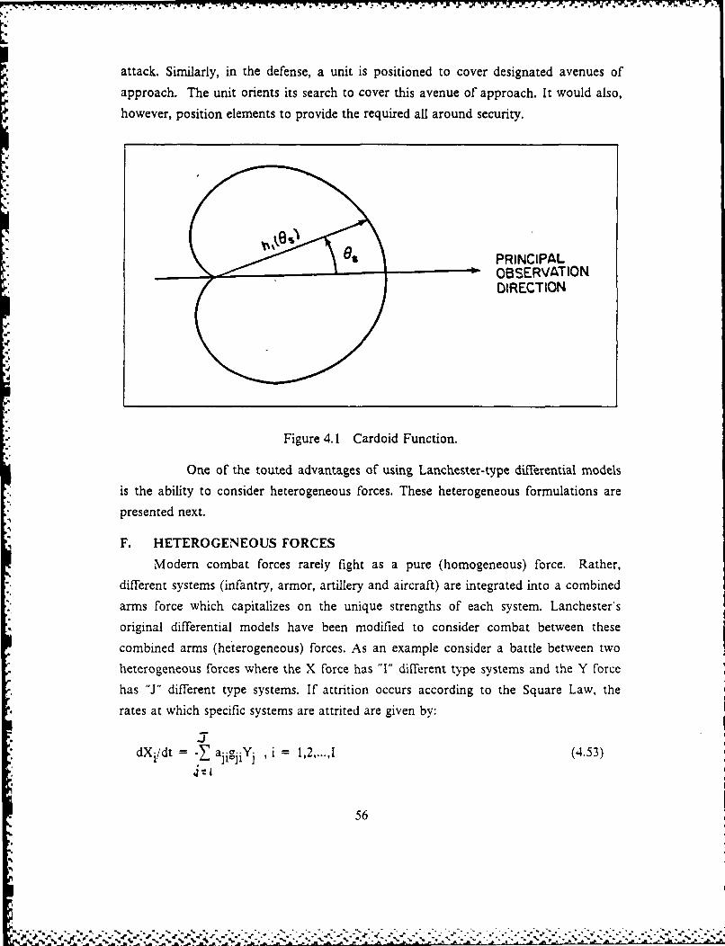
attack. Similarly, in the defense, a unit is positioned to cover designated avenues ofapproach. The unit orients its search to cover this avenue of approach. It would also,
however, position elements to provide the required all around security.
PRINCIPALOBSERVATIONDIRECTION
Figure 4.1 Cardoid Function.
One of the touted advantages of using Lanchester-type differential modelsis the ability to consider heterogeneous forces. These heterogeneous formulations are
presented next.
F. HETEROGENEOUS FORCES
Modem combat forces rarely fight as a pure (homogeneous) force. Rather,different systems (infantry, armor, artillery and aircraft) are integrated into a combined
arms force which capitalizes on the unique strengths of each system. Lanchester'soriginal differential models have been modified to consider combat between thesecombined arms (heterogeneous) forces. As an example consider a battle between two
heterogeneous forces where the X force has "I" different type systems and the Y force
has "J" different type systems. If attrition occurs according to the Square Law, therates at which specific systems are attrited are given by:
-TdXi/dt - - ajig jiY , i - 1,2,...,I (4.53)
56
A.

and
dY1 /dt -- -XbikijXi , J - 1,2,...,J (4.55)j ] 1i
with
Xi(O) =Xio and Y1(0) -- 0
Where
X i= remaining number of i-type X elements at time, tYj= remaining number of j-type Y elements at time, t
a- = rate at which the jth type Y force system attrits
one of the ith type system of force X
bij = rate at which the ith type X force system attritsone of the jth type system of force Y
gji = proportion (probability) that the jth type Y system
engages the ith type X system, 0 - gji - 1.0.
kij = proportion (probability) that the ith type X system
engages the ]th type Y system, 0 < kij < 1.0.Xio = initial number rf i-type X systemsYjo= initial number of j-type Y systems.
(note: gji -< 1.0 and k- -1.0)
Similar heterogeneous formulations apply to the Linear Laws. As suggested
previously with homogeneous attrition models, the heterogeneous formulations could
be used to model target acquisition between opposing combined arms forces.
One of the difficulties that may arise in using heterogeneous formulations (bothin attrition and acquisition models) is the problem of determining the allocation
proportion coefficients for cach opposing system combination. Some coefficients may
be obvious, such as the proportion of anti-aircraft radar systems devoted to detecting
approaching infantry. An example of a more subtle case, though, involves ground
surveillance radars (GSR). These sensors are capable of detecting both motion and
sound. Typically they are employed to cover large sectors and alert the unit to
approaching enemy forces. They do not search exclusively for any specific type of'
57
e-e. e., rQ 5 Q~' ,.--

enemy force, but rather search for both dismounted infantry and armored forces. To
assign a proportion of the available GSR to detecting only a single type target wouldincorrectly degrade its performance against a combined arms force. A solution may beto estimate the acquisition coefficients from the output of a high resolution model.
These estimated acquisition coefficients will reflect the rates at which each specificsensor-type acquires each target-type. The allocation proportion coefficients should beintrinsic to the estimated acquisition coefficients.
This thesis begs the question of how allocation proportion coefficients are finallydetermined. It is presumed that if the decision is made to use a heterogeneousLanchester-type formulation to model target acquisition, follow-on studies will beconducted to resolve problems surrounding the assignment of the allocationcoefficients. The next chapter presents a methodology by which acquisition coefficientscan be estimated from the output of a high resolution combat simulation or field trialresults.
4.4
58

V. DETERMINATION OF ACQUISITION COEFFICIENTS
A. THE ACOUXSITION-RATE COEFFICIENT'S RELATIONSHIP TOACQUISITION TIMEThe basic Lanchester-type model of attrition is of the form:
dX/dt = -c(t,X,Y)dY/dt = -PI(t,X,Y).
In this case the attrition rate function, ux(t,X,Y), may depend on time, the X force level
and the Y force level. For example, using the square law formulation:
dX/dt = -aY
dY/dt = -bX
4. the attrition rate functions are:
a(t,X,Y) = -aY
and
jI(t,X,Y) = -bX
where a and b are the attrition rate coefficients.
Most current calculations of attrition rate coefficients are based on the premise thatthe coefficients are the reciprocal of the expected time for an individual firer to kill a
single target. Therefore, when using a Lanchester-type model for acquisition it would
seem reasonable to use the reciprocal of the expected time for a searcher to acquire a
target as the acquisition coefficient. The Lanchester acquisition-rate coefficient is given
by:
a = lE[Txy] (5.2)
where E[*] is the mathematical expectation and Txy is the time (a random variable)
for a Y searcher to acquire an X target.
Using this dcfinition, the determination of the expected time to acquire a target isthe fundamental calculation required for arriving at the acquisition-rate coefficients in
a Lanchester-type model.
5 9

-- W
B. JUSTIFICATION FOR USING THE RECIPROCAL OF THE TIME TOACQUIRE
This justification follows an argument presented by Taylor [Ref 10:pp. 397-437]
concerning the use of the reciprocal of the expected time to kill a target as the
attrition-rate coefficient in a homogeneous Lanchester-type combat model.1. Acquisition as a Continuous Time Markov-Chain
Let acquisition be modelled as a continuous time Markov-Chain. The numberof unacquired combatants on each side is a non-negative, integer random variable
where:
m0 = the initial number of X force combatants
no = the initial number of Y force combatants
M(t) = a random variable, the number of unacquired X force combatants at time
t with realization denoted as m
N(t) = a random variable, the number of unacquired Y force combatants at time t
with realization denoted as n
G(t,m,n) = the rate at which the X force is acquired
H(t,m,n) = the rate at which the Y force is acquired
2. Development of The Forward Kolmogorov Equations
Let the individual component state probability vector be denoted as, P(t,m,n),
which is the probability that at time, t, the number of unacquired X force combatants
is m and the number of unacquired Y force combatants is n given that at time, t = 0,
the number of unacquired X force combatants was mo and the number of unacquircd
Y force combatants was n0. Further assume that the probability that one X force
combatant is acquired in the interval [t,t + h] is:
G(t,m,n) x h
and that the probability that one Y force combatant is acquired in the interval [t,t 4- h]
is:
Il(t,m,n) x h
and finally, the probability of a total of more than one acquisition on either one or
both sides during the interval It,t+ hi is:
o(h)
a function 11*) is o(h) if lim fh)h = 0).
The initial conditions for the forward Kolmogorov equations are:
(O,m,n) = 1 ,for in =in and n n 0
00
.4... , = o , * - -, . . . ' . . . ' , . ' , . - - . . , . . - . . . " . " . . " .. . .

P(O,m,n) - 0 ,for m c mo or n e no
and
P(t,m,n) = 0 ,for m > mn or n > no.
Now for0 < m m noand0 < n : no
P(t+ h,m,n) = P(t,m,n) x {l-[G(t,m,n) x h+ H(t,m,n) x hJ}
+ P(t,m+ l,n) x G(t,m+ l,n) x h
+ P(t,m,n+ 1) x H(t,m,n+ 1) x h + o(h)
or since there is some probability that the state vector will be in the status, M(t + h)
m and N(t + h) = n, then one of four mutually exclusive events must have occurred:
(1) M(t) = m and N(t) = n and there were no acquisitions during the interval
[t,t + h]
(2) M(t) = m+ l and N(t) = n and one X force combatant was acquired in the
interval [t,t + h].
(3) M(t) = m and N(t) = n+ 1 and one Y force combatant was acquired in the
interval [t,t + hj.
(4) two or more acquisitions took place during [t,t + h].
Multiplying through and rearranging the term results in:
[P(t+ h,m,n)-P(t,m,n)]/Ih = P(t,m+ l,n) x G(t,m+ l,n)
+ P(t,m,n+ 1) x lH(t,m,n+ 1)
- P(t,m,n) x G(t,m,n)
- P(t,m,n) X I I(t,m,n).
Taking the limit as h -0 results in the following:
dP(t,m,n),dt = P(t,m+ l,n)xG(t.m+ l,n)+ P(t,m,n+ l)xlI(t,m,n+ 1) (5.4)
-P(t,m,n)x[G(t.m,n) + l-(t,m,n)]
Equation 5.4 is the forward Kolmogorov equation for the probability
distribution of the number of unacquired combatants on both sides during the courseof the battle. This equation applies only for the initial conditions given above. The
Kolmogorov equations have a slightly different form at the boundaries. The full set of
Kolmogorov equations is given by Taylor [Ref. 10:p. 408].
61
h.

- -~ -j -7 K.- --W_;O '''W'
3. Distribution of Times Between Acquisitions
To determine the distribution of times between acquisitions the probability of
no acquisitions in a time interval, 10,t], is considered. For mn = moand n =no then:
dP(t,m0 5no)/dt = -[G(t,m0 ,n0 ) + H(t,m0,n0 )] x P(t,mo,,nc,) (5.6)
with the initial condition P(0,m0 ,n0) = I.
This is an ordinary differential equation of the form:dP/dt + Q(t) x P(t) = 0 where
Q(t) = G(t,m0 ,n0 ) + H(t,m0o,%)and with a solution given by:
tP(t,rn0 ,n0 ) = exp{.J(G(s,m0 ,n0 ) + H(s,nio,n0 )] ds} (5.8)
Now if TI is the time at which the first acquisition occurs when measured from the
beginning of the battle then:
Prob[TI > tJ = P(t,raao,no) (5.10)
which is the probability of no acquisitions in the interval, IO,tJ. The distribution
function , F'-I'(t), for the time to the first acquisition is given by:
F-rl(t) I - Probf TI > t J or
tFTIt - exp(-5 [G(s,mn 0n)+ H(s,rno,n0 )] ds} 5.2
TI~t)
If the acquisition rate functions are independent of time then the acquisitionprocess is a continuous-time Markov chain with stationary transition probabilities. The
rate functions may be written as:
G(t,m.0,,n,) =A(m 05,n,)
I l(t,rn0 ,n0 ) =B(m 0,n0 )
and then
FT I(t) =I c xp{ - [A(m 0,n0 ) + B(rno,n 0 )J x t (5.14)
a. 62

Equation 5.14 can be recognized as the distribution function of an exponential
probability density function with parameter:
= [A(mo,n 0 +B(m 0 ,no) 1 .
Taylor [Ref. lO:p. 4281 shows that this result can be generalized to any time interval,ft,t+sJ, so that the time between acquisitions is given by the exponential density
function:
fs(s) = [A(m,n)+ B(m,n)] x exp{-[A(m,n)+ B(m,n)]s} (5.16)
where S = time between two successive acquisitions. The expected time between
acquisitions is:
E[Ts] = l/[A(m,n)+B(m,n)] (5.18)
Now, given that an acquisition has occurred the probability that an X force combatant
was acquired is:
A(m,n)/[A(m,n) + B(m,n)]
and the probability that a Y force combatant was acquired is:
B(m,n),I[A(m,n) + B(m,n)I
Finally, given that at time, t, the Markov chain is in state, M(t) = m and N(t) =n,
then the probability that an acquisition occurs on or before time, t + s, and that an X
force combatant is acquired is:
A(m,n), [A(m,n) + B(m,n) J[A(m,n) + B(m,n)]exp{-[A(m,n) + B(m,n)]T} dt0
Similarly for a Y force acquisition:S
B(m,n)1 [A(m,n) + B(m,n)j f[A(m,n) + B(m,n)lexp{-[A(m,n) + B(m,n)jt} dr
The above results form the computational basis for determining the
acquisition rates in a Lanchester-type model of acquisition. The next section discusses
a procedure to estimate the acquisition rate coefficients from the output of high
resolution simulations or field trials.
63
6 A".-4 z" o";.";" .". : ',.:'.' .*'& '' -', '; 2. --. :.,,Z . ,. . .. ?., -,.".",.3.." . . .

C. MAXIMUM LIKELIHOOD ESTIMATION OF ACQUISITION-RATE
COEFFICIENTS
The actual determination of numerical values for attrition coefficients has been
accomplished by two approaches [Ref. 12:pp. 1,4]:
(1) A statistical estimate based on data generated by a detailed Monte-Carlo
combat simulation.
(2) An analytical submodel of the attrition process.
This section presents a maximum likelihood estimation procedure for the
acquisition coefficients of a Lanchester-type model of acquisition. It is based on the
work done by Clark [Ref. I1] while developing his "Combat Analysis Model",
COMAN, and presented by Taylor [Ref 12:pp. 125,140]. The use of this procedure
presupposes that data concerning the time between acquisitions is available from either
a high resolution, Monte-Carlo simulation or field trials. This data is then used to
compute statistical estimates of the acquisition-rate coefficients.
To illustrate the procedure the continuous-time Markov-chain analog of the
deterministic, homogeneous, Lanchester square law will be used. Specifically let
acquisition be modelled by:
dX/dt = -A(m,n) = -aY with X(0) = X o
dY/dt = -B(m,n) = -bX with Y(0) = Yo'
where
a = number of X targets acquired/(Y observer x time)
b = number of Y targets acquired/(X observer x time)
Assume that a high resolution, Monte-Carlo simulation has been run until K
acquisitions have occurred and that the time between successive acquisitions of X force
and Y force combatants has been recorded. The time of the kth acquisition ( for k = I1,2,...,K ) will be a random variable, Tk, with realization tk. Starting the battle at t =0
the total length of the battle will be TK. Then using the corresponding continuous-time
Markov-chain model and the notation previously dcfincd, let
mk = the number of unacquired X force combatants just after the occurrence of
the kth acquisition
nk = the number of unacquired Y force combatants just after the occurrence of
the 0t acquisition
6,4
z """ " ""-""1" '-. " "" "- ". ". "; '-""." -',." - -' -" . -. ". '. ".',"',.'%" .'_2_'.'_ ' ' ", _' ' ; 11'11' -" _ -%,2 .." .l, .z .. .. .

S = time between consecutive acquisitions (a random variable) with realization
denoted as s
CXk I if the kt h acquisition is an X force combatant and 0 otherwise
cYk I if the kt h acquisition is a Y force combatant and 0 otherwiseK
cX= CXk
KCYt = CYk
kI
Note that
CXk X CYk = 0
CX k + CYk = I
and
CXt + CY - K.
From the continuous-time Markov-chain model developed in the preceding
sections Taylor [Ref. 12:pp. 130,131] shows that the time between acquisitions is an
exponentially distributed random variable with density function given by:
fs(s) = (an+bin) X expl-(an+bm)s (5.20)
The maximum likelihood function for the sequence of acquisitions is the product
of each of the individual components. For the kth acquisition the individual
contribution for the acquisition of an X force combatant is:
(ank. 1) exp[-(ankl 1 + bmk.1)(tk- tkl)1
The contribution for the acquisition of a Y force combatant is:
(bmk. 1) exp[-(ank. 1 + bmk-l)(tk- tkl)]
Combining the two components and using the indicator variables results in:
C C(ankl)CV,(bmkl) Ckcxp[-(ank-l + bnik-l)(tk- tk-l)]
Thercfore the likelihood function is givcn by:
65

L(a,b) = I(ank. 1)k (bmk- I)Ck exp[-(ank- 1 + bmk- 1)(tk-tk- 11 (5.22)
Taking the natural logarithm of the likelihood function and maximizing it with respect
to the parameters, a and b, results in the following estimators for the square law
formulation:'
Ka = cXt/ [ nk - tk-l) (5.24)
^ Kb = CYt /[ mk-l(tk.- tkl)l (5.26)
These coefficients are the ratio of the total number of acquisitions of the combatants
on one side to the total humber of acquisition time units directed against that force bythe opposing side. Thus the dimensions of the coefficients are acquisitions per time.
Taylor [Ref. 12:pp. 136,138] shows that this result is a special case and may be
generalized. When the rate functions are of the form:
A(m,n) = a x ga(m,n) (5.28)
B(m,n) = b x gb(m,n) (5.30)
where
a and b are acquisition coefficientsand
ga(m,n) and gb(m,n) are functions which depend only on the state that the
Markov process is in (i.e. they are independent of time)
the estimators are then given by:
a = Cxt I ga( k-l,nk-0(tk - tk-l)] (5.32)
b = cY [ gmk-,nk - tkl) (534)k- i
66

The maximum likelihood estimation method was illustrated for homogeneous
forces. Its applicability also extends to heterogeneous forces without extensive
modification. The estimated parameters are those for acquisition of the ith type X
combatant by the jth type Y combatant and vice versa. This requires detailed data on
the successive acquisition times for all types of combatants on one side by all types of
combatants on the opposing side. The result will be a set of estimated parameters aij
and bj, i for all (i,j) and (j,i) pairs .
These coefficients will depend upon the rate by which specific target types are
acquired by each sensor type in the high resolution model. Thus the allocation
proportion coefficients of a heterogeneous Lanchester-type formulation are contained
in the acquisition coefficients which have been estimated from a high resolution
combat simulation.
D. THE RATE AT WHICH ACQUIRED AN ACQUIRED TARGET RETURNSTO THE UNACQUIRED STATEOne of the fundamental differences between the attrition and acquisition
processes is the regeneration of targets. In attrition models a destroyed target is
permanently eliminated from the battlefield (this excludes those targets which are
subsequently repaired and return to the battle). The acquisition process differs
significantly in this respect; a target may make multiple shifts between the acquired and
unacquired states during the course of the battle. An acquisition model based on a
Lanchester-type formulation could account for this phenomenon by including a
'replacement" coefficient. The basic Lanchester formulation for acquisition which
includes targets returning to the unacquired state would have the form:
dX'dt = -a(t,X,Y) + K(t,X,Y)and
dY dt = -jl(t,X,Y) + X(t,X,Y)
where K(t,X,Y) and ).(t,X,Y) are the acquisition-loss functions and measure the
respective rates at which the X and Y forces return to the unacquired state.
In order to determine the rate at which combatants revert to the unacquired state
the factors which cause the loss of acquisition nmust be determined. These Vactors can
be grouped into three general categories.
Physical - acquisition is lost due factors such as violation of range thresholds (the
taret moves beyond maximum range or closes to under minimum rane , loss of'
line of' sight, the cessation of the signature required for continued acquisition, ctc.
67
." " . . - "' , - " " . . , - . .4' " " , -' ° - - , ' -" - ,. " . " - . " - ' . " - " " , ' " . .

yi - . -° . J.°V -. •'. .-
I"'
Attrition - either the target is destroyed or the sensor(s) responsible for its
continued acquisition is destroyed. In the first case the target is, in effect,
removed from the battlefield and the population of combatants which are
available to be acquired is reduced. The second case removes the sensor,
however, the target may subsequently be re-acquired by the remaining sensors.
Time - the failure to take timely action against a target or to re-confirmed the
acquisition of a target may cause the loss of acquisition. As an example. field
artillery units generally consider a target to be acquired even if a sensor is not
currently monitoring the target. If, however, the targeting information is not
acted upon or the acquisition re-confirmed within a reasonable period of time,
the target is considered lost. It is as if the sensor "forgets" that it has acquired the
target.
The rate at which targets return to the unacquired state would be a function of
the above factors and would have individual components comprised of each. By
modifying a high resolution combat simulation, such as the Simulation of Tactical
Alternative Responses, (STAR), so as to maintain a record of targets returning to the
unacquired state, it would be possible to obtain a numerical estimate for the values of
the individual components. The acquisition-loss coefficient could in-turn be obtained
from the individual components. This would allow the use of a Lanchester-type
formulation to model acquisition in a large scale combat simulation like ALARM.
E. SUMMARY
This chapter has shown that the reciprocal of the expected time to acquire
targets is a reasonable choice for the acquisition coefficients of a Lanchester-type
formulation of acquisition in a large scale combat model. Further, numerical estimates
of acquisition coefficients can be arrived at by the method of maximum-likelihood
estimation. The ability to arrive at estimates of acquisition coefficients based on data
generated from high resolution, Monte-Carlo simulations, in which established target
detection models are used, is an important result. Additionally the same technique can
be employed to obtain the acquisition-loss coefficients. The successful implementation
of these techniques will be required in order to use a Lanchester-type formulation for
target acquisition in ALARM.
68

VI. THE INTELLIGENCE MODULE AND DECISION-MAKING INALARM
A. A. DECISION-MAKING IN ALARM* The preceding chapters of this thesis have concentrated on developing the
conceptual basis for the Intelligence Module and the related function of target
acquisition. The key to the decision making process in ALARM is the
inter-relationships between the Execution, Planning and Intelligence Modules. This
chapter illustrates the relationships between the modules by presenting an extended,
worked example.
ALARM will use an approach to decision-making which has been referred to by
Kilmer [Ref 3:p. IlI as "future state decision making" as opposed to "current state
decision making". Current state decision-making focuses on deciding at time, ti, what
actions should be taken at time, ti + t. based on the perceived situation at ti. Future
state decision-making, as an alternative, uses the expected situation at time, ti+ t, as
the basis for current decisions. This approach requires algorithms to predict the future
states based on the situation at time. t , and to forecast how the situation will change
over time. Kilmer has developed a ,et of' exponential functions known as the
Generalized Value System, GVS, which will be used to represent the future states of
battlefield entities in ALARM. [he GVS methodology is based on two major premises:
* The value of an entity at a particular point in time to a given hierarchical level is
dependent on how useful the entity is at that time and on the availability of' the
entity. Power is the measure of that usefulness. I lhe metric for power in GVS is
called Standard Power Units (STAPOWSi.
'The power of an entity that is not ready to execute its assigned mission is
discounted. As the entity moves closer in time to being able to accomplish the
assigned mission its power grows e\ponentlall.
An entity's power is situational and may be classilied as:
* Basic Inherent Power (B1P) - the inherent power possessed by an entit% at full
strength when it is in position to engage its most likely opponent.* Adjusted Basic Inherent Power ( ,llA ! P - the B P of' an cntit adjuted fur the
specific mission and condition of the entity at the prcent tine, tp.
69
i-

7-,."-- - - -.
S Predicted Adjusted Inherent Power (PABIP) - the ABIP that an entity is
predicted to have at time, ti, given its current state at time, tp, where ti > tp.
The PABIP for an entity is calculated using:
PABIP(tiltp) - ABIP(tp) x exp[.L(ti.tp)] (6.2)
where L is assumed to be constant during the period (tp,ti).
* Situational Inherent power (SIP) - the PABIP of an entity which is adjusted for
availability. For times before an entity is in available to perform its mission it is
the PABIP discounted by an exponential factor. For times after the entity is inposition to accomplish its mission it is the PABIP adjusted for attrition, if
required.
The results of the SIP calculations and the graphs of the SIP curves, whichreflect the predicted power of the entities involved in the battle, are the primary devices
used for future state decision-making as presented in this worked example. In order to
maintain simplicity several assumptions will be made.
* The time used in the example is the simulation clock time and is measured in
hours from t = 0. It will advance in 1 hour steps.* When a unit is moving its rate of advance is constant. This allows simulation
time to be used in the formulas for determining power.
* Units lose power according to the situation based on the following rate schedule:
a. 0.0 per hour for stationary units not engaged in combat with enemy
forces.
b. .05 per hour for units which are moving but not engaged in combat with
enemy forces.c. .10 per hour x the number of enemy units which are being fought
for units which are engaged in combat.
A unit's power at any given time can be found by using:
Power(t) = Power(ti) x expiL(t-t) ] (6.-)
where L is the the natural logarithm of( 1.0 - the loss rate) and t ti.
70
..,,',. ,"...-',. ,." *.,,',',, ...., ,. .. . '' ... ," . -".", " -*. . . ''' .'. '. ' .. . " .. i, ,

For example a unit with an initial power = 100 , at to = O,moves for three
hours unopposed and then engages in combat with two enemy units for one hour. The
loss of power is:
power 100 X exp[(ln.95) X 3] = 85.74 , for t = 3 and
' power 85.74 x exp[(In.80) X 1] = 68.59 , for t = 4.
* Only ground maneuver units can engage more than one enemy unit
simultaneously. Artillery and attack helicopter units can only engage one enemy
unit at a time.
* There are no synergistic effects as a function of force mix. The power of a
composite unit is merely the sum of the power of each individual component
unit.
• Individual units cannot be split. They must be assigned as a whole to a single
mission.
* Intelligence about enemy activities held by senior units will only be made
available to a subordinate when the enemy unit crosses into the subordinates
area of interest. Information on enemy units outside of a unit's area of interest
cannot be obtained.
Since the purpose of this example is to illustrate the logical relationships between
the Intelligence, Execution and Planning Modules certain functions of each will be
treated as "black boxes". Only the results of target acqui;ition, attrition and movement,
which are accomplished in the Execution Module, will be reported. Similarly. the
decisions reached in the Planning Module will be implemented without detailing the
methodology by which they were reached. The algorithms by which the intelligence
estimates are arrived at has not been developed. As a consequence predicted enemy
courses of action, which would be generated within the IEP of the Intelligence Module,
are also presented without detailing the actual process.
Finally, as a disclaimer, this example does not preport to rellect correct tactical
doctrine, rather it is contrived in order to present various functions of the Intelligence
Module.
B. A WORKED EXAMPLE
The example will concentrate of the flow of information and the subsequent
decisions within a Blue Armored Brigade.
71

1. Scenario
A Blue Armored Brigade is defending an area against an approaching Red
Motorized Rifle Division. The mission of the Blue forces is to prevent the Red forces
from advancing past the rear boundary of the Brigade for the next 12 hours. The
combat entities involved in the battle along with their ABIPs are given in Table 5. The
ABIPs of the Blue forces reflect that they are being employed in a defensive operation.
The advantage accruing to a defending unit is assumed to triple its BIP. A diagram of
the battlefield, showing the Areas of Interest and Influence, is at Figure 6.1. A
cartesian coordinate system is used for reporting and example calculations.
TABLE5
INITIAL ABIP OF COMBAT UNITS
ENTITY TYPE ABIP
X1 Tank Battalion 3000X2 Tank Battalion 3000X3 Tank Battalion 1000X4 Attack Heli. Co. 2400X5 Field Artillery Btry. 1800YI Motorized Rifle Reg. 2100Y2 Motorized Rifle Reg. 2100Y3 Motorized Rifle Reg. 3000Y4 Tank Regiment 3600
2. Initial Situation, t 0
The position of the forces at time, ti = 0, is shown in Figure 6.2a. Red
Regiments YI and Y2 have just finished fighting the Blue Divisions covering force and
are in the process of resupplying and reorganizing. Red Regiments Y3 and Y4 areabout to enter the Blue Brigade's area of interest. The Red plan calls for Y3 to
onduct a supporting attack in Blue sector I at t = 3 while Y4 attacks in Blue sector 2
at t = 2 . After resupplying YI and Y2 will also attack in scctor 2 at t = 4 in M
attempt to overwhelm the defending forces (the attack time is the time at which the
attacking force reaches the Blue Brigade's area of influence).
The Blue Brigade has deployed its subordinate units so that XI is defending insector I and X2 is defending in sector 2. X3 is the Brigade's reserve and is positioned
so that it can move to reinforce either XI or X2 within one hour. The initial Blue plan
72
U., " ' . - . ". -" . . " ' . . .-.- . . . -. . - s ' - - ''' " - '- i':" - ." .. i' " -" " % '" - " " " " ; ' ' ' ' ' ' ' '

: . ,+ -, . *- -i. ,- - . -,, +'- ,- . .,i '' -. -," . '.-- .- "..-' .,, . . ., . ." -
, , ', .--- ' - - , - ,-. 4 -. ,i- , ,
00o 0 o5
C14 (N 0
01 0
W - WU r- I,::
co 0oNmON o
ca 00
00
Figure 6.1 Diagram of Battlefield.
calls for X4, the attack helicopter company, to support Xl while X5, the artillery
battery, will be used to support X2. Plots of the true projected SIP curves for the initial
plans of both forces are shown in Figure 6.3. The plots are presented for the Brigade
sector as a whole (Figure 6.3a) and for sectors I and 2 separately (Figure 6.3b and c-!espectively). Notice that overall the Brigade has the needed combat power to defeat
the Red forces, however, the initial Blue plan does not correctly assign the subordinate
units. Specifically sector 2 does not possess adequate combat power to successfully
oppose the attacking Red forces.
In accordance with the assumptions the Blue Brigade's knowledge about the
Red forces is limited to Y I and Y2 which are located within its area of interest. For the
purposes of this example a shortened version of the target vector, which was
introduced in Chapter 111, will be used to present the Blue Brigade's perception of the
Red forces. Specifically the following components will be used:
0 11= targets true identity
73
"i ,..-..,Z.. , j.;.,.: - .". .., .,',:...''...'. ,'.'.'," -" " " "."."" . " " -, , , " . " " " - -
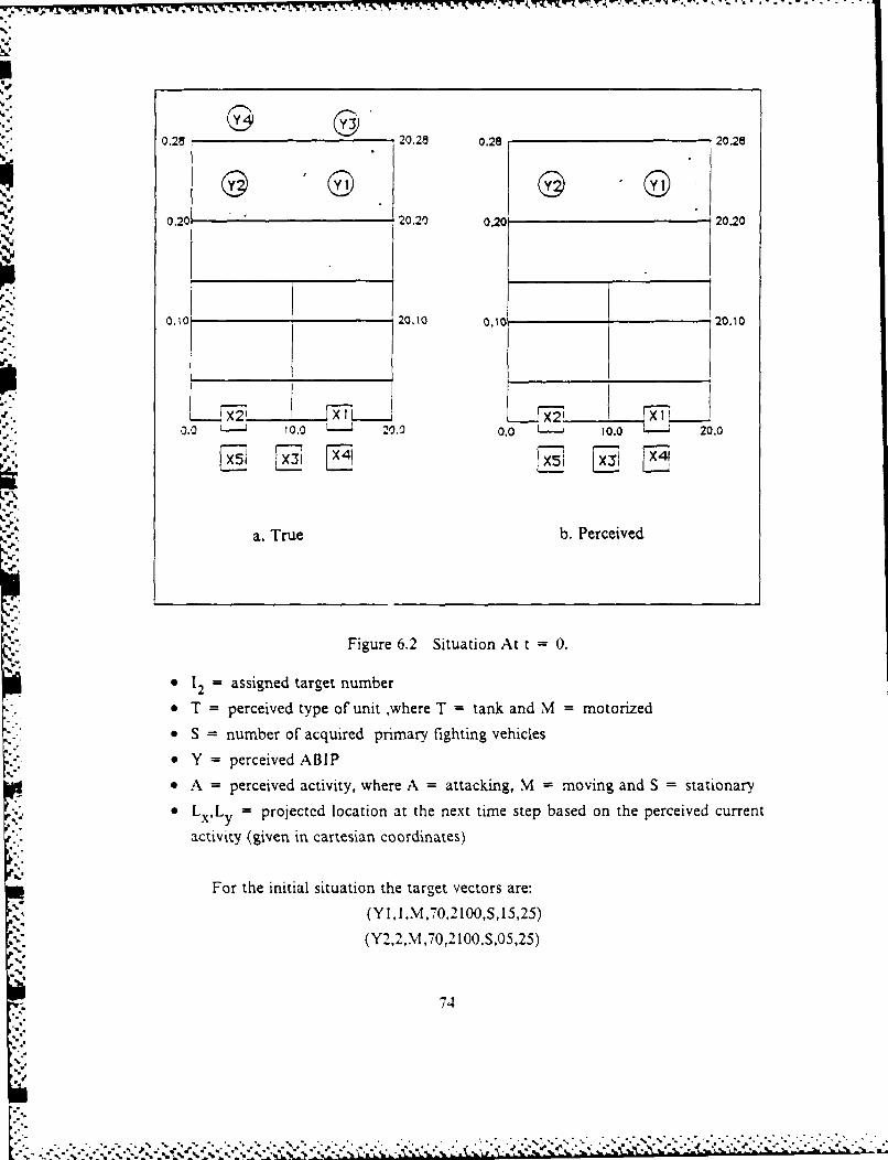
0.28 20.28 0.28 20.28
0.20 20.20 0.20 20.20
0.1 20.10 0.10 20,10
, 10.0 ' _ 20.0 0.0 10.0 20.0
[.X51 [X:51 _X4
a. True b. Perceived
Figure 6.2 Situation At t = 0.
• 12 = assigned target number
* T = perceived type of unit ,where T = tank and M = motorized
• S number of acquired primary fighting vehicles
y = perceived ABIP
• A = perceived activity, where A = attacking, M = moving and S = stationary
LxLy = projectcd location at the next time step based on the perceived current
activity (given in cartesian coordinates)
For the initial situation the target vectors are:
(Yl,I.M ,70.2100,S,15,25)
(Y2,2,M ,70,2 100,S,05,25)
74
S.
|o.o
|,-. . . . . .. - . -. - . . .- ., ., -. -/ ' ,. ' . - .. .- ..". . " ... ".".'.-.'" '..- . ''- .. '. C ""/ -" ' - . " '" ""

II-) U
Oat 0o I =I
Fiur 6.) PoetdPwrC rvsfrIiilPas
(fli' 75

Blue intelligence estimates that YI and Y2 will not be completed resupplying before t
= 3 and that they will attack in sectors I and 2, respectively, at t = 4. The Blue
perception of the battlefield at t = 0 is shown in Figure 6.2b. The associated SIP
curves are displayed in Figure 6.4. Based on the these power curves the Planning
Module determines that the currently assigned forces can defeat the projected attacks
in each sector.
3. Situation at t = 1
The position of the forces at time, t = 1, is shown in Figure 6.5a. Red
Regiments Yl and Y2 are continuing to resupply . Red Regiments Y3 and Y4 have
entered the Blue Brigade's area of interest and are advancing to attack in accordance
with the initial Red plan.
The Blue Brigade's CIP has received the following information vectors from
the Execution Module:
(YI,M,70,S,I5,25)
(Y2,M,70,S,05,25)
(Y3,M,20,M,14,24)
(Y4,T,30,M,06,24)
The information vector is a subset of the target information vector components where:
0 It = targets true identity
* T = type of unit
9 S = size of unit
* A = activity
9 Lx and Ly = the reported location in cartesian coordinates.
Following the flow diagram for target aggregation (Figure 3.2) the CIP
sequentially processes each information vector and aggregates or creates new target
vectors as required. For the purposes of the example a standard Red regiment will have
100 primary fighting vehicles. The circular error probable (CEP) associated with the
Blue Brigade's ability to locate a Red regiment is 1.774 and is assumed to be
preportional to the number Red vehicles where:
CEP = 0.01774 x S.
For brevity, only the aggregation tests will be shown for the information
vectors concerning Y3 and Y4 . The level of significance will be set for a = 0.05; the
9 5 th quantile of the X42 distril ution is 5.991.
76
* %.

[ '-
//
tz, ~ ~ 009 0#0L
/ !
// '
Oo
0
///I
//
000JL OO 0 00U;0SM SdYdSIo
m0/
K /o dI
= /
000U- 1 0009 000 0
SSM~dVIS
Figure 6.4 Perceived Power Curves For t 0.
77

10
0.28 20.28 0.28 20.28
0.20 20.20 0.20- 20.20
0,101 20.10 0.1 20,10
L _ I _7
X21 -1 l_ IX___0.0 1 10.0 ' 20.0 0.0 10.0 - 20.0
a. True b. Perceived
Figure 6.5 Situation at t = 1.
a. Tests on Information Vector Y3.
(1) Type test - a search of the current target vectors reveals a type match withtarget 1.
(2) Proximity test
D' (15-14) 1 + (25-24) 1 = 2.0
a2 = (1.2418/1.774)2 = 0.49
= (0.3548/1.774)2 - 0.04
so
T = 2.0/(0.49 + 0.04) = 3.77
For an ct = .05 the null hypotl,esis cannot be rejected. The
information vector is judged to be a separate report about target 1.
(3) Adjusted Location - the adjusted location of target I is calculated
78

using:
r, = 70/(70 + 20) = 0.78
r2 = 20/(70 + 20) = 0.22
s, = 0.7/(0.7 + 0.2) = 0.78
s2 = 0.2/(0.7 + 0.2) = 0.22
so
X' =[15 x (0.78+0.22)/2 + 14 x (0.22+0.78)/21 = 14.5
Y' = [25 x (0.78 + 0.22)/2 + 24 x (0.22 + 0.78),/21 = 24.5
The intermediate target vector is:
(YI,1,M,70,*,S,14.5,24.5) .
This intermediate target vector is passed to the IEP which predicts the probable
course of action of the enemy unit. Based on this the ABIP and the next
position of the unit are estimated. The final target vector is:
(Y 1,I,M,70,2 100, S,14.5,24.5)
b. Tests on Information Vector Y4.
A search of the current target vectors fails to reveal a type match with
information vector Y4. A new intermediate target vector is created and passed to the
IEP which returns the final target vector:
(Y4,3,T,30,1000,M, 10,17)
This new combat information is reported to the division CIP. The final result
of the target aggregation process is the set of three target vectors:
(Yl,l,M,70,2100,S,14.5,24.5)
(Y2,2,M,70,2100,S,05,25)
(Y4,3,T,30, 1000,M,10,17)
which represent the Blue Brigade's perception of the battlefield.
Using these target vectors the IEP concludes that the new target is a tank
battalion which will be used to locate the defending Blue forces in sector 2 and initiate
the attack; Y2 will follow Y4 and attempt to break-through. The perceived situation isshown in Figure 6.5b and the corresponding SIP curves in Figure 6.6. Based on the
perceived situation there has been a slight increase in the threat to the Brigade.
I Iowever, there still appears to be no dilficultlv in dealing with the attacks by usin, the
initial Brigade plan. No changes are ordered by the Planning Module.
79
"d
- -, , % , % % % o ,' ' ° - ° , , " . * , , - , " , - • , . % -. • , j " . .'.'* ". K. % . .
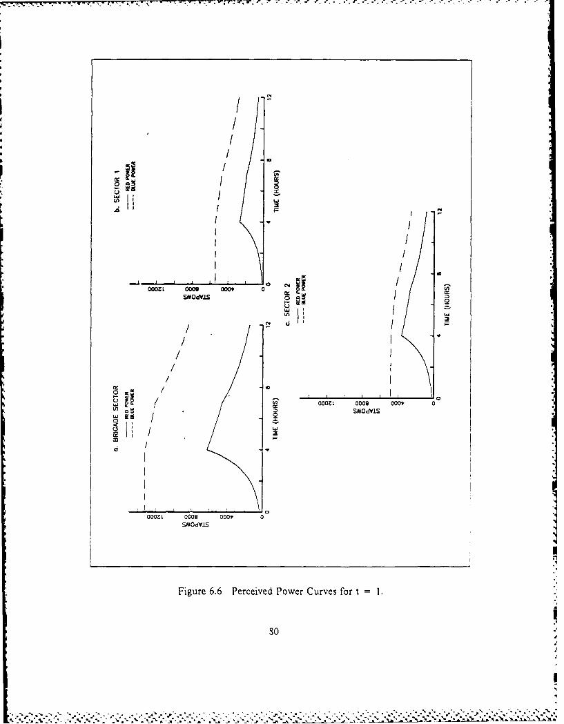
7i -
/
0
I
IiI / -
i / i
0O0L 0009 O00 P 00 C4
SMOdV.LS 0
00
/ ~
//
/
OjU00Z L 000 000t 0
0000 L O000 000' 0
Lfl SMdVVIS
Figure 6.6 Perceived Power Curves for t =1.
80
4." '.""-"".' "- ." -,- .', .- ,.-.'W 0.'--' .- - . . - , . -, ., --. , --- :.". ".., .'..b :.. -, .,-,

4. Situation at t = 2
The position of the forces at time, t = 2, is shown in Figure 6.7a.. Red
Regiments Y1 and Y2 are continuing to resupply . Red Regiments Y3 and Y4 have
entered the Blue Brigade's area of influence and are advancing to attack in accordancewith the initial Red plan.
0.28 20.28 0.28 20.28
YC2I)
_ _ _ _ I .0.201 - 20.20 0,201 20.20
"" '2 X2 !
0.0 10.0 20.0 0.0 0.0 - 0.0
*X51 3 x41 x5 X3:
a. True b. Perceived
Figure 6.7 Situation at t = 2.
The Blue Brigade's CIP has received the following information vectors :r1::
the Execution Module.
(YI,M,70,S,15,25)
(Y2,.,l ,0,S.05.25)
(Y3.M.30,A, 12, I S)
(Y4,T,60.A.09,).
• %%
............ ..... t -..........

Again, considering only the information vectors for Y3 and Y4, the the target
aggregation procedure is initiated by the CIP. Based on the type test Y3 is tested for
proximity to target vector 1, the closest similar type unit. This produces a test statistic
of T = 94.47, which results in the rejection of the null hypothesis and the creation of
the following intermediate target vector
(Y3,4,M,30,*,A,12,18).
Similarly a type test for Y4 matches it to target vector 3. The proximity test,which compares the reported location of Y4 to the estimated location of target 3,
returns a test statistic of T = 2.78, which does not allow the the null hypothesis to be
rejected. The existing target vector 3 is updated to reflect the new combat information.
The intermediate target vector is:
(Y4,3,T,*,A,09,17).
These intermediate target vectors are processed by IEP which returns the
following full set of target vectors which now include the estimated power and next
location of the enemy units
(YI,I,M,70,2100,S,15,25)
(Y2,2,M,70,2100,S,05,25)
(Y4,3,T,60,2500,A,05,06)
(Y3,4,M,30,1000,A,07,07).
This new set of target vectors reflect the IEP estimate that target 3 consists of
two tank battalions while target 4 is a motorized rifle battalion. It concluded that Y3
and Y4 will attack in sector 2. There is no change in the forecasted activities of YI and
Y2. Based on the SIP curves generated by the IEP, the Planning Module uses X5, the
artillery battery, to place long range fires on Y4. The combat information about Y3
and Y4 along with thc notification of the initiation of combat action against Y4 is sent
to the division CIP. The Blue Brigade's perception of the battlefield is displayed in
Figure 6. 7b.
1 he SI P curves, which havc been adjusted to reflect the use of X5, are shown
In I nture O.,. Notice that overall the Blue Brigade perceives that it holds a decided
, ' . ifo%%ever, within sector 2 the attacking Red forces will achieve a slight
. i.,: 'c lut hclore t = 4 which they will maintain throughout the duration of the
I ., J, is judged not to be significant and no additional Blue forces are
. . .., . , . ;.. , .' . .)

%,.
%.
a,.-4
OO- 00 OO
SM~dYI
'I I -
occ
%o

5. Situation at t = 3
The position of the forces at time, t 3, is shown in Figure 6.9a. Red
Regiments Yl and Y2 have completed resupplying and are moving to the attack. Red
Regiment Y3 has entered the battalion area of interest for sector 1 while Y4 has
entered the area of influence for the battalion in sector 2. Y4 is still under attack by
X5 and has been automatically engaged by X2 when its area of influence was entered.
The Blue Brigade's CIP has received the following information vectors from
the Execution Module.
(YI,M,80,M,15,25)
(Y2,M,80,M,05,25)
(Y3,M,90,A,15,12)
(Y4,T,90,A,05,07).
The CIP conducts the target aggregation tests which results in the following
intermediate target vectors
(Yl,l,M,80,*,S,I5,25)
(Y2,2,M,80,*,S,05,25)
(Y4,3,T,90,*,A,05,07)
(Y3,4,M,90,*,A,15,12).
Using this set of target vectors the IEP estimates that Y4 is a tank regiment
and Y3 is a motorized rifle regiment. The predicted course of action for the Red forces
has Y3 attacking in sector 1 and supported by Y1 which will arrive at t = 4. Y4 is
attacking in sector 2 and will be supported by Y2 which is projected to enter the battle
at t = 4. The IEP adjusted target vectors are:
(Y l,,M,80,2400,M, 15,15)
(Y2.2,M,80,2400,M,05,15)
(Y4.3,T,90,3300,A,05,07,
(Y3,4,M ,90,2700,A, 15.07).
The updated combat information on Y3 and Y4 is send to the division (Ti1.
.Additionallv the (1lP of XI is notified of the arrival Y3 within its area of interest. lhe
pcrnci scd hattcliceld situation is shown in I igure 6.9b.
Ihe I'Ianrung \Nlodule orders X4, the attack helicopter conipany. to engage
Y I lie ,cr .ci ed SIP curves whIL result from these Modifications In the BfLIC plin
.1rc it I :1ure I [hle Blue IlrIgadc still bhcoces that it hIds an overall ddantaee L r
lic H r2 iIc ,C t r as a while. Ihe prl oc,.!cd p,)er of the Red Ircs in ,ector I has
.......

0.28 20.28 0.28 20.28
0.2 - 0.20 0.20 20.20/V
:_ _0,__0 2 0 , 1 0 0 .1 02 ,2
0.0 i0.0 20 .0 0,0 0.0 2.0
X31 EXX4 Z:
a. True b. Perceived
Figure 6.9 Situation at t = 3.
increased but is below that of the Blue forces defending in that sector. In sector 2 the
Red forces are still projected to hold a slight advantage. This advantage does notwarrant the commitment of the reserve battalion, X3.
6. Situation at t = 4
The position of the forces at time, t = 4, is shown in Figure 6.1 Ia. Red
Regiments YI and Y2 have entered the area of' interest for sector 2 and are moving to
support Y4 which continues to attack in that sector. Red Regiment Y3 has entered :!-e
area of influence for sector I and has been engaged by X I. X5 still attacks Y-1 with
S5
• "" "-" "-"-L., I'.'' -","-".'.'. ''-" "''-"",'".""."'-":,'"" "'-'" "'" '"-",,;'.'"." '". " ." .'' ", ." " '" '"-' "-"-'-'% -'""'- ","-''- p" '1' " p J 4, . °-- o' ' a." • ,
",% % aa \% . " . ' % "% % ".', , " °. . . " . " ".". . " '. " " ,', % .1

Pi
/ /
II
86
I /•

artillery fire while X4 continues to engage Y3. The Blue Brigade's CIP has received the
following information vectors from the Execution Module:
(Y1,M,80,A, 10,13)
(Y2,M,80,A,05,12)
(Y3,M,90,A,15,07)
(Y4,T,90,A,05,07).'. ,I
' 0.28 20.28! 0.28 20.28
0.20. 120.20 0.20 20.20
Y Y
0, o1 20.10 0. o 1 0 20.10
- i
X21 L 7F- _ _1 _
0.0 - 0.0 - 20.0 0.0 - 0. - 20.0
-XT X3'
a. Unadjusted b. Adjusted
Figure 6.11 Situation at t =4.
The CIP conducts the target aggregation tests which results in the tollowing
intermediate target vectors:.~~( -1. ( ,I , SO,., 10, 13)
°* (-. (Y2 2,M.,SO,',.\, )512)
.(Y4.3,T90,,,,5,o 7)
S7
-"'- 87 * ff.:V'A.i ~ -.- ~ ~~... 5'-
" . A

•-V .I- . . .
(Y3,4,M,90,*,A, 15,07).
The IEP now estimates that the main attack will come in sector 2 and will
consist of Red Regiments YI,Y2 and Y4. The attack by Y3 will be a supporting attack
designed to prevent XI from maneuvering to assist in sector 2 and to siphon off
potential Blue reserves. The IEP adjusted target vectors are:
(YI,I,M,80,2400,M,03,07)
(Y2,2,M,80,2400,M,07,07)
(Y4,3,T,90,3300,A,05,07)
(Y3,4,M ,90,2700,A, 15,07).
The subordinate battalion CIPs are sent the adjusted combat information for their
respective sectors. The Blue Brigade's perception of the battlefield mirrors the true
situation for the first time during the battle.
The SIP curves for t = 4 are shown in Figure 6.12. It is apparent that the
Blue Brigade still has more power than the combined Red forces in the Brigade's
sector. However, the Red forces committed to sector 2 possess significantly more
power than the Blue forces defending it. Without adjustments to the Blue plan the Red
forces will be able to achieve a break-through in sector 2.
The Planning Module commits the reserve battalion, X3, to sector 2
Additionally X4 is ordered to support sector 2 by continuing to attack YI. The
modified battlefield situation is shown in Figure 6.1lb and the adjusted SIP curves
sector for this modified plan are displayed in Figure 6.13. Now the power of the Blue
Brigade has been alined so that it is superior to the Red power in both sectors. Based
on these projected power curves the Blue Brigade will be able to prevent the Red forccs
from penetrating past the Brigades rear boundary and therefore successfully complete
its mission.
C'. SIAINIARY
I hils example dklC,1?btr,,tcN the itttcr-rellitiori prs bctwcen the I \ck:,Uti .
Irc :ccrite and IIi:mlre \()Idu s ul \I .\R\ I lhe kc% point l rhe dct:,ii::;:e
m~i .£ ri)Lss i th IlIJ1itie \I0111C ll zd the e~tiniatioii [1rOir ;ri 11he 11 P'
f l- I C .1 '. ie l!:i. :..! LC \In.. ie , tlito :l tI c \rkuive c tic . oth ied ) the
%., ,r, oriC

*r.r
smodyl(
0/
L0~ 000 000w 0 09 OOISMDcft'J.S LS
Lf ' m
)OO.. )OR =
F 01 ereiedP ,we (ur-e fr

00
C. t ODV
/ I dVL0 .
Door L /09 00
SMOdVLS
Fiur 0.1 zdP wr uvsfrt 4
/duse L.Ac
902
.01 'J
/e 4.r f
/eAe or -- A-i

:~2.7- Y ~1:6 V V V~~~r * ~ . ~ *-- ~.. -
either aggregate or not aggregate target vectors can result in the perception of the
battlefield being distorted from ground truth. Since the intelligence estimate prepared
by the TEP uses the target vectors this can result in an incorrect prediction of the
enemy courses of action. The plans prepared by the Planning Module, which are in
turn based on the intelligence estimate, may then be faulty and fail to correctly assign
combat assets to cope with the enemy situation.
Subsequent information from the Execution module, as well as intelligence from
senior units and combat information will tend to act as a correcting influence on the
perceived state of the battlefield. The relationships between the modules can therefore
be viewed as dynamic and self-correcting. As more reliable information is made
available to the IEP the perceived state of the battlefield should approach ground
truth.

,
VII. SUMMARY/FUTURE DIRECTIONS
A. SUMMARYThis thesis has developed the conceptual foundation for the Intelligence Module
of the AIRLAND RESEARCH MODEL (ALARM). The relationship between theExecution, Planning and Intelligence Modules has been detailed. Methodologies bywhich the Intelligence Module can accomplish required functions were explored. The
following are the key results.* The Intelligence Module will consist of two sub-modules; the Combat
Information Processor (CIP) and the Intelligence Estimate Processor (IEP).
* Information from the Execution Module will be routed to the appropriate CIPbased on task-force hierarchy.
e The CIP receives raw information from the Execution Module and using thealgorithms developed in Chapter I II produces combat information. This combatinformation forms the basis for the intelligence estimate and subsequent plans
developed by the Planning Module.e The IEP will be tasked with developing an intelligence estimate. Specific
functions of the IEP include matching targets to specific organizations in theenemy's order of battle, predicting the enemy's course of action and preparingthe SIP curves for the enemy forces.
e Decisions will be based on the predicted future state of the enemy forces.
e The Execution Module will produce "ground truth" information, there is nobuilt-in error. Deviations from ground truth arise because of the decision
algorithms used by the IEP and CIP sub-modules.
* Target acquisition, which is a function of the lFxecution Module, could possibly
be successfully modelled usine a Lanchester-tvpe Formulation. [he lormul, tion
must include components Ior acquisitlon as well ad the los of ,IcqIsition.
* The coefficicnts for a l.anchestcr-t, re formulation o aqLjtiofl Lould heobtained by a maximum likelihood est mtion proc cdure. I11c output o high
rc,,olution combat ,imulations or fiWlJ trials would be Cquircd f r the ctiniar,,0
procedure.
, -,

In summary, the concept of the Intelligence Module developed in this thesis
provides a basis for future research and study. The development of decision algorithms
for the IEP are dependent on current ongoing projects. The successful completion of
the terrain and avenue of approach models will open the way for future development of
the intelligence estimation process. The required CIP functions are well identified. This
thesis represents only the initial effort in identifying methodologies to accomplish the
required tasks. Finally, Lanchesterian models of acquisition appear to hold great
promise for modeling acquisition in ALARM.
B. FUTURE DIRECTIONS
There are several areas which require future research for the continued
development of the Intelligence Module. The use of decision templates in the
preparation of intelligence estimates needs to be fully explored. The current use of
these templates by intelligence officers is a widespread and accepted practice. They
provide a convenient starting point for developing decision algorithms to identify
enemy organizations and predict their courses of action.
The successful use of a Lanchester-type formulation of acquisition is dependent
upon developing estimates for the process coefficients. This will require either
modifying an existing high resolution combat simulation or creating a new one for zhe
specific purpose of obtaining times between acquisitions. In order to be applicable to a
wide variety of situations several terrain and force nix scenarios should be explored. A
data base to draw upon must be developed.
Finally, the algorithms used in the CIP must be selected, either trom thoc
presented in this thesis or developed else where. These algorithms should be con cr'c4A
to computer code and the initial steps of integrating them into A I.AR\l accorip1\hcJ
.,>. ,*.**j % .- '.- ,4 .. . -, -% °. o-

LIST OF REFERENCES
1. Department of the Army, FM 100-5, OPERATIONS, 20 August 1982.
2. Hartman, J.K., Parry, S.H., and Schoenstadt, A.L. Air/and Research Modelpae resented to the Military Operations aesearch Society, Naval
ostgraduate School, Monterey, California, June 1984.
3. Kilmcr, Robert, Using the Generali2ed Value S stem for Future State DecisionMIaking M.S. Thesis, Naval Postgraduate SchooI, Monterey, California,March 1986.
4. Lindstrom, Robin, Field Artillery Mfodule for the Air/and Research Wodel, M.S.* Thicsis, Naval Postgraduate School, Monterey, California, March 1986.
5. Hlartmnan. i.K.. Lecture N\otes in H-ig~h Resolution Combat Mfodelling,ug~ublished paper, Naval Postgraduate school, Monterey, California, June
195.
De1)partment of the Army, 1)ARCOM-P 706-101, Engineering Designllapidhook, November 1977.
Ko L)p man. Bernard Gj.. 0Kl.G Report 56 Search and Screening, Department ofthe Nav . washiniton, D.C., Januan. 1946.
I 1 r r1, T. 1 .Le, rure .\)w ~~in A vizgreiaed Combat Modeling unulse\ alPo,,tj~aduatc SchIiooI \fonierey, California ulie1985.
.1 itcs ( 1 , 'z Ir,' trat'm l'bdeI/j'ii \lilitarv A\pplicationsC )r~crt Kes clcr,-h Sotietv ot Amierica, Arlington. \ irginia. I 91o.
I I ..::'~ ( L~'r ~'.i~'~ ' U r 1'r. /. 1, \Iilitarv ApplicationsNi <>, ()c ~ Rc: ,'.~k Sos.,, :'If Arf.nicrica, A'rlington, Viru'inia, M1arch
I :~.I, Kn \l ., ':-x <s l PrccdIngs 24th. NlilitarN
Uin
So it .l A mc.. . . . ....n../(,n
.. . . . . .. . . ... - V

INITIAL DISTRIBUTION LIS F
1. Defense Technical Information (enterCameron StationAlexandria, Virginia 22304-6145
2. L.ibrarv Code 0142Naval-Posteraduate SchoolMonterey, California 93943-50l2
3. Deputy L ndersecretarn of the Armyfor Operations RcsearLhRoom 2E261 PentaeonWashington, D.C. 20310
.1* DirectorU.S. Armv TRADOC Operatiomns Rccji \ ,"White Safids Missile Range. \cw \lc\,,, "
5. CommanderU.S. Army IR.),OC Ant, (Fort Leavenworth. Kan VA, o,'-2
6. DirectorAttn: ir. 1 B \i:,',c II", F .S..'\rTfl\ ( n,.C : c; 1, ' ,, \Bethcda, \l, I "1 1: 'Be!!l3~~ II 'I 1:'
"-' " ~I \ '1 .: .v .. ..*', I: lc.. t:'
- ." .,, i)* : ' . . .
£ -T
7A