Legged Robot State-Estimation Through Combined Forward Kinematicand Preintegrated Contact Factors

Ross Hartley, Josh Mangelson, Lu Gan, Maani Ghaffari Jadidi, Jeffrey M. Walls,Ryan M. Eustice, and Jessy W. Grizzle

Abstract— State-of-the-art robotic perception systems haveachieved sufficiently good performance using Inertial Mea-surement Units (IMUs), cameras, and nonlinear optimizationtechniques, that they are now being deployed as technologies.However, many of these methods rely significantly on visionand often fail when visual tracking is lost due to lightingor scarcity of features. This paper presents a state-estimationtechnique for legged robots that takes into account the robot’skinematic model as well as its contact with the environment.We introduce forward kinematic factors and preintegratedcontact factors into a factor graph framework that can beincrementally solved in real-time. The forward kinematic factorrelates the robot’s base pose to a contact frame throughnoisy encoder measurements. The preintegrated contact factorprovides odometry measurements of this contact frame whileaccounting for possible foot slippage. Together, the two devel-oped factors constrain the graph optimization problem allowingthe robot’s trajectory to be estimated. The paper evaluates themethod using simulated and real sensory IMU and kinematicdata from experiments with a Cassie-series robot designedby Agility Robotics. These preliminary experiments show thatusing the proposed method in addition to IMU decreases driftand improves localization accuracy, suggesting that its use canenable successful recovery from a loss of visual tracking.

I. INTRODUCTION AND RELATED WORK

Legged locomotion enables robots to adaptively operatein unstructured and unknown environments with potentiallyrough and discontinuous ground [1]. The state-of-the-artcontrol algorithms for dynamic biped locomotion are capableof providing stabilizing feedback for a biped robot blindlywalking through sinusoidally varying [2] or discrete [3]terrain; however, without perceiving the environment, theapplication of legged robots remains extremely limited. Ac-curate estimates of the robot’s state and environment areessential prerequisites for both stable control and motionplanning [4], [5], [6]. In addition, real-time performance ofthe state estimation and perception system is required toenable online decision making [7], [8].

Legged robots, unlike ground, flying, and underwater plat-forms, are in direct and switching contact with the environ-ment. Leg odometry involves estimating relative transforma-tions and velocity using kinematic and contact information,which can be noisy due to the encoder noise and footslip [9]. Typically, legged robots are equipped with additionalsensors (IMUs, cameras, or LiDARs) which also provide in-dependent, noisy odometry measurements (shown in Fig. 1).

The authors are with the College of Engineering, University of Michigan,Ann Arbor, MI 48109 USA {rosshart, mangelso, ganlu,maanigj, eustice, grizzle}@umich.edu, with the ex-ception of Jeff Walls who is with Toyota Research Institute.

Fig. 1: Experiments were conducted on a Cassie-series robot designed byAgility Robotics. The biped robot has 20 degrees of freedom, 10 actuators,joint encoders, an IMU, and a Multisense S7 stereo camera.

Therefore, without a sound sensor fusion framework, theestimated trajectory can quickly become inaccurate as aconsequence of significant drift over the traveled distance.

Filtering methods involve estimating the current stateusing all measurements up to the current time [10]. Ex-tended Kalman filters (EKFs) are often used to fuse high-frequency inertial and contact measurements to provide ac-curate velocity, and orientation estimates that are useful forthe stabilizing feedback controller [4], [11]. However, theabsolute position and yaw (rotation about gravity) have beenshown to be unobservable [4], which leads to the unboundeddrift in these states. Re-observing landmarks over time usingvision sensors allows for correcting the position and yawestimates. However, landmark positions are unknown andhave to be estimated alongside the robot’s state. Over time,the accumulation of numerous landmarks can make the EKFcomputationally intractable for long-term state estimationand mapping [12].

In contrast, smoothing methods estimate a discrete tra-jectory of states using all the available measurements [10].Although the comparatively lower update rate may not beuseful for the feedback controller, absolute position and yawestimates can be corrected by relating the current pose to aprevious one through loop closures [13]. This allows for low-drift long-term state-estimation and mapping solutions. State-of-the-art visual-inertial odometry systems [14], and, gener-

ally, Simultaneous Localization and Mapping (SLAM) [15],[16], use graphical models (factor graphs) and nonlinearoptimization techniques to achieve a probabilistically soundsensor fusion framework and real-time performance by ex-ploiting the sparse structure of the SLAM problem [17],[13]. The high-dynamic motion and noise characterizationis captured using preintegration of high-frequency sensorssuch as Inertial Measurement Units (IMUs) [18].

Although the factor graph framework has been successful,most methods heavily rely on visual information and areprone to failure when visual tracking is lost, often due tolighting or scarcity of features. In these scenarios, leg odom-etry is a way to reduce drift; and hereby, the incorporationof contact and encoder measurements into the factor graphframework are addressed. In this paper, we develop twonovel factors that integrate the use of multi-link ForwardKinematics (FK) and the notion of contact between therobotic system and the environment into the factor graphsmoothing framework. The forward kinematic factor relatesa sensor frame (such as a camera or IMU) to a contact framethrough noisy encoder measurements. On the other hand,the contact factor preintegrates high-frequency foot contactmeasurements to describe the contact frame’s movementover time. When combined, these novel factors constrain therobot’s net movement, leading to improved state estimation.In particular, this work has the following contributions:

i. An FK factor that incorporates noisy encoder measure-ments to estimate an end-effector pose at any time-step;

ii. rigid and point preintegrated contact factors that relatethe contact frame pose between successive time-stepswhile accommodating noise from foot slip;

iii. integration of leg odometry into the factor graph smooth-ing framework;

iv. real-time implementation of the proposed FK and prein-tegrated contact measurement models on a Cassie-seriesbiped robot.

Section II provides the required preliminaries includingthe notation and mathematical prerequisites. We formulatethe problem and our factor graph approach in Section III.Section IV explains forward kinematic modeling. The for-ward kinematic factor is developed in Section V. Rigid andpoint contact factors are derived in Sections VI and VII,respectively. Simulation and experimental evaluations of theproposed methods on a 3D biped robot (Fig. 1) are presentedin Section VIII. Finally, Section IX concludes the paper andprovides future work suggestions.

II. PRELIMINARIES

In this section, we present preliminary materials necessaryfor the developments in the following sections. We firstestablish the mathematical notation where we assume readersare already familiar with basics of Lie groups, Lie Algebra,and optimization on matrix Lie groups [19], [20], [21]. Also,as this work is partly motivated by on-manifold IMU prein-tegration, we adopt the notation from [14], where possible,so that readers can connect the two papers conveniently.

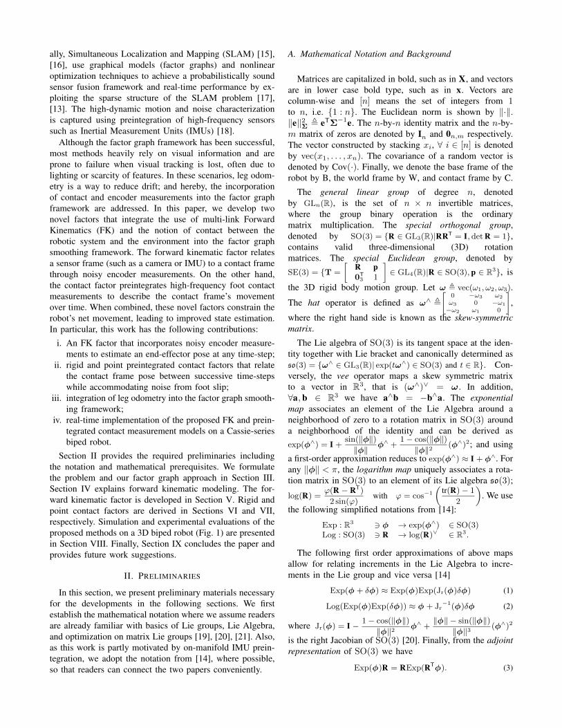
A. Mathematical Notation and Background

Matrices are capitalized in bold, such as in X, and vectorsare in lower case bold type, such as in x. Vectors arecolumn-wise and [n] means the set of integers from 1to n, i.e. {1 : n}. The Euclidean norm is shown by ‖·‖.‖e‖2Σ , eTΣ−1e. The n-by-n identity matrix and the n-by-m matrix of zeros are denoted by In and 0n,m respectively.The vector constructed by stacking xi, ∀ i ∈ [n] is denotedby vec(x1, . . . , xn). The covariance of a random vector isdenoted by Cov(·). Finally, we denote the base frame of therobot by B, the world frame by W, and contact frame by C.

The general linear group of degree n, denotedby GLn(R), is the set of n × n invertible matrices,where the group binary operation is the ordinarymatrix multiplication. The special orthogonal group,denoted by SO(3) = {R ∈ GL3(R)|RRT = I, det R = 1},contains valid three-dimensional (3D) rotationmatrices. The special Euclidean group, denoted by

SE(3) = {T =

[R p0T

3 1

]∈ GL4(R)|R ∈ SO(3), p ∈ R3}, is

the 3D rigid body motion group. Let ω , vec(ω1, ω2, ω3).

The hat operator is defined as ω∧ ,

[0 −ω3 ω2

ω3 0 −ω1

−ω2 ω1 0

],

where the right hand side is known as the skew-symmetricmatrix.

The Lie algebra of SO(3) is its tangent space at the iden-tity together with Lie bracket and canonically determined asso(3) = {ω∧ ∈ GL3(R)| exp(tω∧) ∈ SO(3) and t ∈ R}. Con-versely, the vee operator maps a skew symmetric matrixto a vector in R3, that is (ω∧)∨ = ω . In addition,∀a,b ∈ R3 we have a∧b = −b∧a. The exponentialmap associates an element of the Lie Algebra around aneighborhood of zero to a rotation matrix in SO(3) arounda neighborhood of the identity and can be derived asexp(φ∧) = I +

sin(‖φ‖)‖φ‖ φ∧ +

1− cos(‖φ‖)‖φ‖2 (φ∧)2; and using

a first-order approximation reduces to exp(φ∧) ≈ I + φ∧. Forany ‖φ‖ < π, the logarithm map uniquely associates a rota-tion matrix in SO(3) to an element of its Lie algebra so(3);

log(R) =ϕ(R − RT)

2 sin(ϕ)with ϕ = cos−1

(tr(R)− 1

2

). We use

the following simplified notations from [14]:

Exp : R3 3 φ → exp(φ∧) ∈ SO(3)Log : SO(3) 3 R → log(R)∨ ∈ R3.

The following first order approximations of above mapsallow for relating increments in the Lie Algebra to incre-ments in the Lie group and vice versa [14]

Exp(φ + δφ) ≈ Exp(φ)Exp(Jr(φ)δφ) (1)

Log(Exp(φ)Exp(δφ)) ≈ φ + Jr−1(φ)δφ (2)

where Jr(φ) = I − 1− cos(‖φ‖)‖φ‖2 φ∧ +

‖φ‖ − sin(‖φ‖)‖φ‖3 (φ∧)2

is the right Jacobian of SO(3) [20]. Finally, from the adjointrepresentation of SO(3) we have

Exp(φ)R = RExp(RTφ). (3)

B. Modeling Noise and Optimization on Matrix Lie Groups

We model the uncertainty in SO(3) by defining a noisedistribution in the tangent space and then mapping it toSO(3) via the exponential map [22], [14]; R = RExp(ε)and ε ∼ N (0,Σ), where R is a given noise-free ro-tation (the mean) and ε is a small normally distributedperturbation with zero mean and covariance Σ. Throughapproximating the normalization factor as constant, thenegative log-likelihood of a rotation R given a measure-ment R distributed according to the defined perturbationis L(R) ∝ 1

2‖Log(R−1R)‖2Σ = 1

2‖Log(R−1R)‖2Σ which is a

bi-invariant Riemannian metric. For the translation part ofSE(3), noise can be characterized using the usual additivewhite Gaussian noise assumptions.

Solving an optimization problem where the cost functionis defined on a manifold is slightly different from the usualproblems in Rn. The tangent vectors lie in the tangent space.As such, a retraction that maps a vector in the tangentspace to an element in the manifold is required [21]. Givena retraction mapping and the associated manifold, we canoptimize over the manifold by iteratively lifting the costfunction of our optimization problem to the tangent space,solving the reparameterized problem, and then mapping theupdated solution back to the manifold using the retraction.For SO(3), the exponential map is this retraction. For SE(3)we adopt the retraction used in [14]:

RT (δφ, δp) = (RExp(δφ),p + Rδp), vec(δφ, δp) ∈ R6. (4)

III. PROBLEM STATEMENT AND FORMULATION

In this section, we formulate the state estimation problemof the legged robot. The biped robot is equipped with a stereocamera, an IMU, joint encoders, and binary contact sensorson the feet. Without loss of generality, we assume the IMUand camera are collocated with the base frame of the robot.In current state-of-the-art visual-inertial navigation systems,the state includes the camera pose and velocity along withsystem calibration parameters such as IMU bias [14]. Inthe factor graph framework, independent measurements fromadditional sensors can be incorporated by introducing addi-tional factors based on the associated measurement models.Foot slip is the major source of drift in leg odometry; assuch, to isolate the noise at the contact point we augmentthe state at time-step i to include the contact frame poseof both feet (in the world frame) Ci , {RWC,l(i)}2l=1 anddi , {WpWC,l(i)}

2l=1. However, without loss of generality, all

following derivations are for a single contact frame. Thus,the state at any time-step i is represented as:

Si , {Ri, pi, vi,Ci, di, bi} (5)

where Ri , RWB(i) is the base orientation, pi , WpWB(i) is thebase position, vi , WvB(i) is the base velocity, and bi , b(i)

is the IMU bias. In addition Xk ,⋃ki=1 Si denotes the state

up to time-step k.Let Lij ∈ SE(3) be a perceptual loop closure measure-

ment relating poses at time-steps i and j (j > i) computedfrom an independent sensor, e.g. using a point cloud match-

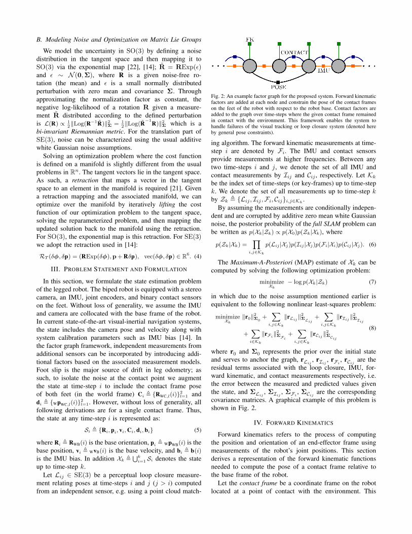
Fig. 2: An example factor graph for the proposed system. Forward kinematicfactors are added at each node and constrain the pose of the contact frameson the feet of the robot with respect to the robot base. Contact factors areadded to the graph over time-steps where the given contact frame remainedin contact with the environment. This framework enables the system tohandle failures of the visual tracking or loop closure system (denoted hereby general pose constraints).

ing algorithm. The forward kinematic measurements at time-step i are denoted by Fi. The IMU and contact sensorsprovide measurements at higher frequencies. Between anytwo time-steps i and j, we denote the set of all IMU andcontact measurements by Iij and Cij , respectively. Let Kkbe the index set of time-steps (or key-frames) up to time-stepk. We denote the set of all measurements up to time-step kby Zk , {Lij , Iij ,Fi, Cij}i,j∈Kk

.By assuming the measurements are conditionally indepen-

dent and are corrupted by additive zero mean white Gaussiannoise, the posterior probability of the full SLAM problem canbe written as p(Xk|Zk) ∝ p(X0)p(Zk|Xk), where

p(Zk|Xk) =∏

i,j∈Kk

p(Lij |Xj)p(Iij |Xj)p(Fi|Xi)p(Cij |Xj). (6)

The Maximum-A-Posteriori (MAP) estimate of Xk can becomputed by solving the following optimization problem:

minimizeXk

− log p(Xk|Zk) (7)

in which due to the noise assumption mentioned earlier isequivalent to the following nonlinear least-squares problem:

minimizeXk

‖r0‖2Σ0+∑

i,j∈Kk

‖rLij‖2ΣLij

+∑

i,j∈Kk

‖rIij‖2ΣIij

+∑i∈Kk

‖rFi‖2ΣFi

+∑

i,j∈Kk

‖rCij‖2ΣCij

(8)

where r0 and Σ0 represents the prior over the initial stateand serves to anchor the graph, rLij

, rIij , rFi, rCij are the

residual terms associated with the loop closure, IMU, for-ward kinematic, and contact measurements respectively, i.e.the error between the measured and predicted values giventhe state, and ΣLij

, ΣIij , ΣFi, ΣCij are the corresponding

covariance matrices. A graphical example of this problem isshown in Fig. 2.

IV. FORWARD KINEMATICS

Forward kinematics refers to the process of computingthe position and orientation of an end-effector frame usingmeasurements of the robot’s joint positions. This sectionderives a representation of the forward kinematic functionsneeded to compute the pose of a contact frame relative tothe base frame of the robot.

Let the contact frame be a coordinate frame on the robotlocated at a point of contact with the environment. This

Fig. 3: The contact frame is separated from the robot’s base frame by Nlinks. Cassie (left) has 7 links between the base and the bottom of thetoe. A simpler, planar biped (right) is shown to demonstrate the forwardkinematics.

contact frame is separated from the robot’s base frame, by Nlinks. These N links are assumed to be connected by N − 1revolute joints, each equipped with an encoder to measurethe joint angle. The vector of encoder angles is denotedby α ∈ RN−1. In total, this amounts to N + 1 frames,where frames 1 and N + 1 are the base and contact framerespectively, as shown in Fig. 3. The forward kinematics canbe computed through a product of homogeneous transforms:

H(α) =

N∏n=1

Hn,n+1(αn) ,

[fR(α) fp(α)01,3 1

]∈ SE(3) (9)

where fR(α) and fp(α) denote the rotation and position ofthe contact frame (relative to the base frame) as a functionof encoder angles. The relative transformation between linkframes n ∈ [N − 1] and n+ 1 is given by:

Hn,n+1(αn) ,

[AnExp(α†n) tn

01,3 1

](10)

where An ∈ SO(3) and tn ∈ R3 are a constant rotation andtranslation defined by the kinematic model of the robot. Eachjoint is assumed to be revolute with an angle αn ∈ R. Thedagger operator maps a scalar to a vector in R3 based onthe joint’s axis of rotation:

α†n , vec(αn, 0, 0), vec(0, αn, 0), or vec(0, 0, αn). (11)

The final transformation between link frames N and N + 1

is constant and denoted by HN,N+1 ,

[AN tN0T

3 1

]. When (9)

is multiplied out, the orientation and position of the contactframe with respect to the base frame are:

fR(α) = A1N+1(α), and fp(α) =N∑n=1

A1n(α)tn (12)

where the relative rotation between link frames i and j isgiven by:

Aij(α) ,

I for (i, j) ∈ [N ], i = j∏j−1k=i AkExp(α†k) for (i, j) ∈ [N ], j > i

AiNAN for i ∈ [N − 1], j = N + 1.

Changes in joint angles affect the orientation of all linkframes further down the kinematic tree. The following

Lemma shows how the angle offsets propagate through theFK functions which is important for dealing with encodernoise.

Lemma 1 (Relative rotation between two frames [23]). Letβ ∈ RN be a vector of joint angle offsets. The relativerotation between frames i and j can be factored into thenominal rotation and an offset rotation:

Aij(α + β) = Aij(α)

j−1∏k=i

Exp(

ATk+1,j(α)β†k

)(13)

V. FORWARD KINEMATICS FACTOR

The goal of this section is to formulate a general forwardkinematic factor that accounts for uncertainty in joint en-coder readings. This factor can be included in a factor graphto allow estimation of end-effector poses. Here, the end-effector coincides with the contact frame. We note that thisfactor only constrains the relative transformation between thebase and contact frames; therefore, the full utility of thisfactor depends on a separate measurement of the contactframe described in Section VI.

A. Contact Pose through Encoder Measurements

The encoder measurements are assumed to be affected byadditive Gaussian noise, ηα ∼ N (0,Σα).

α(t) = α(t) + ηα(t) (14)

The orientation and position of the contact frame in the worldframe are given by:

RWC(t) = RWB(t)RBC(t)

WpC(t) = WpB(t) + RWB(t)BpC(t).(15)

Rewriting (15) in terms of the state (5) and encoder mea-surements yields:

C(t) = R(t) fR(α(t)− ηα(t))

d(t) = p(t) + R(t) fp(α(t)− ηα(t)).(16)

The isolation of the noise terms in orientation and positionof the contact frame are derived in the following Lemmas.The dependence on time is assumed, so t is omitted forreadability.

Lemma 2 (FK factor orientation noise isolation [23]). Using(12), (13), and (3), the rotation term and the noise quantityδ fR can be derived as:

RTC = fR(α − ηα)

= fR(α)

N−1∏k=1

Exp(−AT

k+1,N+1(α)ηα†k

), fR(α)Exp(−δ fR)

(17)

δ fR = −Log

(N−1∏k=1

Exp(−AT

k+1,N+1(α)ηα†k

))

≈N−1∑k=1

ATk+1,N+1(α)ηα†k

(18)

Through repeated first order approximation, the noise quan-tity δ fR is approximately zero mean and Gaussian.

Lemma 3 (FK factor position noise isolation [23]). Using(12), (13), (1), and anticommutativity of skew-symmetricmatrices, the position term can be approximated as:

RT(d − p) = fp(α − ηα)

≈ fp(α) +

N−1∑k=1

N−1∑n=k

A1,n+1(α)t∧n+1ATk+1,n+1(α)ηα†k

, fp(α)− δ fp

(19)

The noise quantity δ fp is a linear combination of zero meanGaussians, and is therefore also zero mean and Gaussian.

Using these Lemmas, we can now write out the forwardkinematic measurement model:

fR(α) = RTC Exp(δ fR)

fp(α) = RT(d − p) + δ fp(20)

where the forward kinematics noise characterized byvec(δ fR, δ fp) ∼ N (0,ΣF ).

B. Unary Forward Kinematic Factor

The FK factor is a unary factor that relates the robot’s baseframe to an end-effector frame. Using (20), we can write theresidual errors, rFi

, vec(r fRi

, r fpi) from (8), at time ti as

follows.

r fRi= Log

(fR(αi)

TRTi Ci)

r fpi= RT

i (di − pi)− fp(αi)(21)

The forward kinematics noise can be rewritten as a linearsystem: [

δ fRδ fp

]=

[Q(αi)S(αi)

]ηα† (22)

where ηα† , vec(ηα†1 ,ηα†2 , · · · ,ηα†N−1) and the columns ofthe 3× 3(N − 1) matrices Q and S are given by:

Qi(α) = ATi+1,N+1(α)

Si(α) = −N−1∑n=i

A1,n+1(α)t∧n+1ATi+1,n+1(α).

(23)

The covariance can be computed using the linear noise modeland the sensor covariance matrix Σα† describing the encodernoise ηα†:

ΣFi=

[Q(αi)S(αi)

]Σα†

[QT(αi) ST(αi)

]. (24)

The Jacobians for the forward kinematics factor are given inthe supplementary material [23].

VI. RIGID CONTACT FACTOR

This section formulates a contact factor based on theassumption that the contact frame remains fixed with respectto the world frame over time. Slip is accommodated byincorporating noise on the contact frames’ velocities. Whencombined with the forward kinematic factor introduced inSection V, an additional odometry measurement of therobot’s base frame is obtained, which can improve the MAPestimate.

A. Rigid Contact Model

In addition to the encoders, it is assumed that a separatebinary sensor can measure when the robot is in contact withthe static world. If the contact is rigid (6-DOF constraint),then both the angular and linear velocity of the contact frameare zero; i.e CωWC(t) = WvC(t) = 03,1. Therefore,

RWC(t) = RWC(t)(CωWC(t) + ηω(t))∧ = RWC(t)ηω∧(t)

WpC(t) = WvC(t) + RWC(t)ηv(t) = RWC(t)ηv(t)(25)

where ηω ∼ N (03,1,Σω) and ηv ∼ N (03,1,Σv) areadditive Gaussian noise terms that capture contact slip. Thisis similar to the EKF-based approach taken in [4]. Both noiseterms are represented in the contact frame and are rotated toalign with the world frame. Rewriting (25) in terms of thestate vector yields:

C(t) = C(t)ηω∧(t)

d(t) = C(t)ηv(t).(26)

If the robot maintains rigid contact with the world fromt to t + ∆t, Euler integration can be applied to obtain thepose of the contact frame at time t+ ∆t.

C(t+ ∆t) = C(t)Exp(ηωd(t)∆t)

d(t+ ∆t) = d(t) + C(t)ηvd(t)∆t(27)

Integrating from the initial time of contact, ti, to the finaltime of contact, tj , yields:

Cj = Cij−1∏k=i

Exp(ηωdk ∆t)

dj = di +

j−1∑k=i

Ckηvdk ∆t

(28)

where ηωd and ηvd are discrete time noise terms computed

using the sampling time; Cov(ηd(t)) =1

∆tCov(η(t)).

B. Rigid Contact preintegration

We can now rearrange (28) to create relative incrementsthat are independent of the state at times ti and tj .

∆Cij = CTi Cj =

j−1∏k=i

Exp(ηωdk ∆t)

∆dij = CTi (dj − di) =

j−1∑k=i

∆Cikηvdk ∆t.

(29)

Next, we wish to isolate the noise terms. First, we willdeal with the rotation of the contact frame. The product ofmultiple incremental rotations can be expressed as one largerrotation. Therefore,

∆Cij , ∆CijExp(−δθij) (30)

where ∆Cij = I due to the rigid contact assumption.Furthermore, through repeated first order approximation,δθij is approximately zero mean and Gaussian.

δθij = −Log(

j−1∏k=i

−Exp(ηωdk ∆t)) ≈j−1∑k=i

ηωdk ∆t (31)

Now, we can isolate the noise in the position of the contactframe by substituting (30) into ∆dij and dropping the higherorder noise terms.

∆dijeq.(1)≈

j−1∑k=i

∆Cik(I − δθ∧ik)ηvdk ∆t ≈ −j−1∑k=i

ηvdk ∆t

, ∆dij − δdij

(32)

where ∆dij = 0. The noise term, δdij =∑j−1k=i η

vdk ∆t, is

zero mean and Gaussian.Finally, we arrive at the preintegrated contact measure-

ment model:

∆Cij = CTi Cj Exp(δθij) = I3

∆dij = CTi (dj − di) + δdij = 03,1

(33)

where the rigid contact noise characterized byvec(δθij , δdij) ∼ N (0,ΣCij ). More detailed derivations areprovided in the supplementary material [23].

C. Preintegrated Rigid Contact Factor

Once the noise terms are separated out, we can write downthe residual errors, rCij = vec(r∆Cij

, r∆dij) from (8), as

follows.

r∆Cij= Log(CT

i Cj)

r∆dij= CT

i (dj − di)(34)

Furthermore, since both noise terms are simply additiveGaussians, the covariance can easily be computed. If thecontact noise is constant, the covariance is simply:

ΣCij =

[Σω 03,3

03,3 Σv

]∆tij (35)

where Σω and Σv are the continuous covariance matricesof the contact frame’s angular and linear velocities, ηω andηv , and ∆tij =

∑jk=i ∆t.

If the contact noise is time-varying, the covariance canbe computed iteratively. This would be particularly usefulif the noise were modeled to depend on contact pressure.The iterative noise propagation and the Jacobians for therigid contact factor are fully derived in the supplementarymaterial [23].

VII. POINT CONTACT FACTOR

The rigid contact factor can be modified to support addi-tional contact types. For a point contact, the contact frameposition remains fixed with respect to the world frame;however, the orientation can change over time. Therefore,∆Cij 6= I, and subsequently becomes unobservable usingonly encoder and contact measurements. To track the contactnoise appropriately, a gyroscope can be used.

In the following section, the preintegrated contact factor isformulated as an extension to the preintegrated IMU factordescribed in [14]. This approach allows support for pointcontacts in our factor graph formulation.

A. Point Contact Model

A point contact is defined as a 3-DOF constraint onthe position of the contact frame. All rotational degrees of

freedom are unconstrained. Since the relative orientation,∆Cij , is unobservable without the use of a gyroscope, weshall remove this term in the preintegrated contact factor byutilizing the preintegrated IMU measurements. Replacing Ckin (28) with its definition in (15), yields:

dj = di +

j−1∑k=i

Rk fR(αk − ηαk )ηvdk ∆t. (36)

We can rewrite this equation to be independent of the stateat time ti and tj .

RTi (dj − di) =

j−1∑k=i

∆Rik fR(αk − ηαk )ηvdk ∆t (37)

where ∆Rij = RTi Rj =

∏j−1i=1 Exp

((ωk − bgk − η

gdk )∆t

)is the relative rotation increment from the IMU preintegrationmodel [14].

The encoder measurements at time ti are already beingused for the forward kinematic factor (Section V). Therefore,to prevent information double counting, the first term in thesummation can be replaced with the state estimate at time ti.After a first-order approximation of the forward kinematicsfunction, we arrive at the preintegrated point contact positionmeasurement ∆dij and its noise δdij :

RTi (dj − di) ≈ RT

i Ciηvdi ∆t+

j−1∑k=i+1

∆Rik fR(αk)ηvdk ∆t

, ∆dij − δdij

(38)

where, again, ∆dij = 03,1. The full derivation is detailed inthe supplementary material [23].

Up to a first order approximation, δdij is zero mean,Gaussian, and does not depend on the encoder or IMU noise,i.e. it is decoupled [23]. Since the contact measurement isuncorrelated to the IMU / forward kinematics measurementsand all are jointly Gaussian, the measurements are all inde-pendent. Therefore, the point contact factor can be writtenseparately to the IMU factor.

B. Preintegrated Point Contact Factor

Once the noise terms are separated out, we can write downthe residual error:

rCij = r∆dij= RT

i (dj − di). (39)

The noise propagation can be written in an iterative form:

δdik+1 =

{δdik − RT

kCkηvdk ∆t for k = i

δdik −∆Rik fR(αk)ηvdk ∆t for k > i(40)

which allows us to write the covariance propagation as alinear system (starting with ΣCii = 03,3):

ΣCik+1= ΣCik + BΣvdBT (41)

where,

B =

{RTkCk∆t for k = i

∆Rik fR(αk)∆t for k > i.(42)

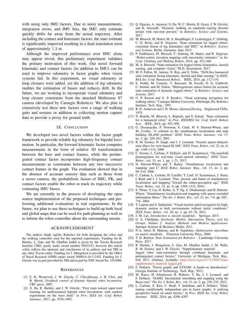
Fig. 4: The cumulative distribution function of the norm of the translationand rotation errors for consecutive poses generated using a model of Cassiein SimMechanics. Measuring error in this way allows us to evaluate thedrift of the different combinations of factors. Forward kinematics, contact,and IMU significantly outperform IMU and even outperforms the local loopclosure (LC) and IMU in some cases.

The covariance of the discrete contact velocity noise ηvdk isdenoted by Σvd. These equations are derived in completedetail in the supplementary material [23].

VIII. SIMULATIONS AND EXPERIMENTAL RESULTS

In this section, we evaluate the proposed method andfactors. We implemented both factors in GTSAM [24] usingiSAM2 as the solver [25]. To handle IMU preintegration weused the implementation built into GTSAM 4 [14], [26]. Bothsimulation and real-world experiments used the Cassie-seriesrobot developed by Agility Robotics (shown in Fig. 1).

A. Simulated Evaluation using SimMechanics

For initial evaluation, we used SimMechanics to simulatea full model of Cassie walking along a curved path. Thesimulator provided true acceleration, angular velocity, jointangle, and contact values as well as ground-truth trajectoryposition and velocity.

We generated IMU measurements by adding Gaussiannoise and bias according to the models described in [14].We also simulated loop closure (LC) measurements usingthe ground-truth trajectory and corrupted them using themethods detailed in Section II-B. These (local) loop closurefactors were added to every other node in the graph in anattempt to simulate the results of visual odometry or scanmatching algorithms. Finally, we added white Gaussian noiseto the contact and joint angle values to generate forwardkinematic and contact measurements. Table I shows the noiseparameters used. A new node in the graph was added everytime contact was made or broken with the environment(approximately 3 per second).

In this experiment, we compared the following combina-tions of factors: IMU, LC and IMU, IMU and Contact/FK,LC and IMU and Contact/FK. Fig. 4 shows the cumulativedistribution function of the norm of the translation androtation errors computed by comparing the relative pose

TABLE I: Simulation Noise ParametersNoise st. dev.

Acceleration 0.0307 m/s2Angular Velocity 0.0014 rad/sAccelerometer Bias 0.005 m/s2Gyroscope Bias 0.0005 rad/sLoop Closure Translation 0.1 mLoop Closure Rotation 0.0873 radContact Linear Velocity 0.1 m/sJoint Encoders 0.00873 rad

Fig. 5: Estimated trajectory of Cassie experiment data using IMU, forwardkinematic, and contact factors. The robot walked in a loop around the lab,starting and ending at approximately the same pose. The video of the ex-periment is shown at https://youtu.be/QnFoMR47OBI. Comparedto the IMU only estimation (dashed red line), the addition of contact andforward kinematic factors significantly improves the state estimate. The end-to-end translation error was approximately 1.3 m.

between consecutive time-steps of the trajectory estimatedby each combination of methods to the ground-truth. Thismetric allows for evaluating the drift of the different com-binations of factors. The translational error is computedin the usual manner. The rotation error is computed using‖Log(R>trueRest)‖.

Forward kinematic, contact and IMU combined, signif-icantly outperform IMU alone. This is partly because thecontact and forward kinematic factors constrain the graphenabling the estimator to solve for the IMU bias. Also, wenote that in translation about 20% of the time the combina-tion of our proposed factors and the IMU outperforms thecombination of the camera and the IMU. Finally, we notethat the combination of all factors is the most successful.

These results suggest that the proposed method can beused to increase the overall localization accuracy of thesystem as well as to handle drop-outs in visual tracking.

B. Real-world

We evaluated our factor graph implementation using realmeasurement data collected from a Cassie-series robot. Thisdata included IMU measurements and joint encoders values.Cassie has two springs, located on each leg, that are com-pressed when the robot is standing on the ground. The binarycontact measurement was computed using measurements ofthese spring deflections. The data was collected at 2KHz.

Using a controller provided by Agility Robotics, wewalked Cassie for about 100 seconds in a loop around a 4.5-meter section of our lab, starting and ending in approximatelythe same location. Figure 5 compares the estimated trajectorycomputed using IMU, contact and forward kinematic factors

with using only IMU factors. Due to noisy measurements,integration errors, and IMU bias, the IMU only estimatequickly drifts far away from the actual trajectory. Afterincluding the contact and kinematic factors, the state estimateis significantly improved resulting in a final translation errorof approximately 1.3 m.

Although the improved performance over IMU alonemay appear trivial, this preliminary experiment validatesthe primary motivation of this work. Our novel forwardkinematic and contact factors (in addition to IMU) can beused to improve odometry in factor graphs when visionsystems fail. In this experiment, no visual odometry orloop closures were added, yet the addition of leg odometryenables the estimation of biases and reduces drift. In thefuture, we are working to incorporate visual odometry andloop closure constraints from the attached Multisense S7camera (developed by Carnegie Robotics). We also plan toextensively test these new factors over a range of walkinggaits and terrains in addition to collecting motion capturedata to provide a proxy for ground truth.

IX. CONCLUSION

We developed two novel factors within the factor graphframework to provide reliable leg odometry for bipedal loco-motion. In particular, the forward kinematic factor computesmeasurements in the form of relative 3D transformationbetween the base and contact frames, while the preinte-grated contact factor incorporates high-frequency contactmeasurements as constraints between any two successivecontact frames in the graph. The evaluation showed that inthe absence of accurate sensory data such as those froma stereo camera, the probabilistic fusion of IMU, FK, andcontact factors enable the robot to track its trajectory whileestimating IMU biases.

We are currently in the process of developing the opensource implementation of the proposed techniques and per-forming additional evaluations in real experiments. In thefuture, we plan to use these techniques to build up both localand global maps that can be used for path planning as well asto inform the robot controller about the surrounding terrain.

ACKNOWLEDGMENT

The authors thank Agility Robotics for both designing the robot andthe walking controller used for the reported experiments. Funding for R.Hartley, L. Gan, and M. Ghaffari Jadidi is given by the Toyota ResearchInstitute (TRI), partly under award number N021515, however this articlesolely reflects the opinions and conclusions of its authors and not TRI orany other Toyota entity. Funding for J. Mangelson is provided by the Officeof Naval Research (ONR) under award N00014-16-1-2102. Funding for J.Grizzle was in part provided by TRI and in part by NSF Award No. 1525006.

REFERENCES

[1] E. R. Westervelt, J. W. Grizzle, C. Chevallereau, J. H. Choi, andB. Morris, Feedback control of dynamic bipedal robot locomotion.CRC press, 2007.

[2] X. Da, R. Hartley, and J. W. Grizzle, “First steps toward supervisedlearning for underactuated bipedal robot locomotion, with outdoorexperiments on the wave field,” in Proc. IEEE Int. Conf. Robot.Automat., 2017, pp. 3476–3483.

[3] Q. Nguyen, A. Agrawal, X. Da, W. C. Martin, H. Geyer, J. W. Grizzle,and K. Sreenath, “Dynamic walking on randomly-varying discreteterrain with one-step preview,” in Robotics: Science and Systems,2017.

[4] M. Bloesch, M. Hutter, M. A. Hoepflinger, S. Leutenegger, C. Gehring,C. D. Remy, and R. Siegwart, “State estimation for legged robots-consistent fusion of leg kinematics and IMU,” in Robotics: Scienceand Systems, Berlin, Germany, June 2013.

[5] P. Fankhauser, M. Bloesch, C. Gehring, M. Hutter, and R. Siegwart,“Robot-centric elevation mapping with uncertainty estimates,” in Int.Conf. Climbing and Walking Robots, 2014, pp. 433–440.

[6] M. A. Bloesch, “State estimation for legged robots–kinematics, inertialsensing, and computer vision,” Ph.D. dissertation, 2017.

[7] M. F. Fallon, M. Antone, N. Roy, and S. Teller, “Drift-free humanoidstate estimation fusing kinematic, inertial and lidar sensing,” in IEEE-RAS Int. Conf. Humanoid Robots. IEEE, 2014, pp. 112–119.

[8] S. Nobili, M. Camurri, V. Barasuol, M. Focchi, D. G. Caldwell,C. Semini, and M. Fallon, “Heterogeneous sensor fusion for accuratestate estimation of dynamic legged robots,” in Robotics: Science andSystems, 2017.

[9] G. P. Roston and E. P. Krotkov, “Dead reckoning navigation forwalking robots,” Carnegie-Mellon University, Pittsburgh, PA, RoboticsInstitute, Tech. Rep., 1991.

[10] B. D. Anderson and J. B. Moore, Optimal filtering. Englewood Cliffs,1979.

[11] N. Rotella, M. Bloesch, L. Righetti, and S. Schaal, “State estimationfor a humanoid robot,” in Proc. IEEE/RSJ Int. Conf. Intell. RobotsSyst. IEEE, 2014, pp. 952–958.

[12] G. Dissanayake, P. Newman, S. Clark, H. F. Durrant-Whyte, andM. Csorba, “A solution to the simultaneous localization and mapbuilding (SLAM) problem,” IEEE Trans. Robot. Automat., vol. 17,no. 3, pp. 229–241, 2001.

[13] R. M. Eustice, H. Singh, and J. J. Leonard, “Exactly sparse delayed-state filters for view-based SLAM,” IEEE Trans. Robot., vol. 22, no. 6,pp. 1100–1114, 2006.

[14] C. Forster, L. Carlone, F. Dellaert, and D. Scaramuzza, “On-manifoldpreintegration for real-time visual–inertial odometry,” IEEE Trans.Robot., vol. 33, no. 1, pp. 1–21, 2017.

[15] H. Durrant-Whyte and T. Bailey, “Simultaneous localization andmapping: part I,” IEEE Robot. Automat. Mag., vol. 13, no. 2, pp.99–110, 2006.

[16] C. Cadena, L. Carlone, H. Carrillo, Y. Latif, D. Scaramuzza, J. Neira,I. Reid, and J. J. Leonard, “Past, present, and future of simultaneouslocalization and mapping: Toward the robust-perception age,” IEEETrans. Robot., vol. 32, no. 6, pp. 1309–1332, 2016.

[17] S. Thrun, Y. Liu, D. Koller, A. Y. Ng, Z. Ghahramani, and H. Durrant-Whyte, “Simultaneous localization and mapping with sparse extendedinformation filters,” The Int. J. Robot. Res., vol. 23, no. 7-8, pp. 693–716, 2004.

[18] T. Lupton and S. Sukkarieh, “Visual-inertial-aided navigation for high-dynamic motion in built environments without initial conditions,”IEEE Trans. Robot., vol. 28, no. 1, pp. 61–76, 2012.

[19] J. M. Lee, Introduction to smooth manifolds. Springer, 2015.[20] G. S. Chirikjian, Stochastic Models, Information Theory, and Lie

Groups, Volume 2: Analytic Methods and Modern Applications.Springer Science & Business Media, 2011.

[21] P.-A. Absil, R. Mahony, and R. Sepulchre, Optimization algorithmson matrix manifolds. Princeton University Press, 2009.

[22] T. D. Barfoot, State Estimation for Robotics. Cambridge UniversityPress, 2017.

[23] R. Hartley, J. Mangelson, L. Gan, M. Ghaffari Jadidi, J. M. Walls,R. M. Eustice, and J. W. Grizzle, “Supplementary material:legged robot state-estimation through combined kinematic andpreintegrated contact factors,” University of Michigan, Tech. Rep.,Feb. 2017. [Online]. Available: https://arxiv.org/src/1712.05873/anc/supplementary-material-legged.pdf

[24] F. Dellaert, “Factor graphs and GTSAM: A hands-on introduction,”Georgia Institute of Technology, Tech. Rep., 2012.

[25] M. Kaess, H. Johannsson, R. Roberts, V. Ila, J. J. Leonard, andF. Dellaert, “iSAM2: Incremental smoothing and mapping using theBayes tree,” The Int. J. Robot. Res., vol. 31, no. 2, pp. 216–235, 2012.

[26] L. Carlone, Z. Kira, C. Beall, V. Indelman, and F. Dellaert, “Elim-inating conditionally independent sets in factor graphs: A unifyingperspective based on smart factors,” in Proc. IEEE Int. Conf. Robot.Automat. IEEE, 2014, pp. 4290–4297.